Radiative MHD Nanofluid Flow Due to a Linearly Stretching Sheet with Convective Heating and Viscous Dissipation

Abstract

This article describes a two-dimensional steady laminar boundary layer flow and heat mass transfer caused by a non-Newtonian nanofluid due to a horizontally stretching sheet. The non-dimensional parameters take into consideration and regulate the effects of convective boundary condition, slip velocity, Brownian motion, thermophoresis and viscous dissipation. The thermal radiation, which affects the flow’s thermal conductivity and the nanofluid’s variable viscosity are also taken into consideration. We propose that a hot fluid could exist beneath the stretching sheet’s bottom surface, which could aid in warming the surface via convection. The physical boundary conditions are non-dimensionalized, as are the governing transport set of nonlinear partial differential equations. By using the shooting approach, numerical values for dimensionless velocity, temperature and nanoparticle concentration are achieved. Distributions of velocity, temperature and concentration are plotted against a number of newly important governing factors, and the outcomes are then provided in accordance with those graphs. Additionally, the local skin-friction coefficient, the local Sherwood number and the local Nusselt number are discussed in order to further clarify and thoroughly explain the current problem. In order to validate the numerical results, comparisons are made with previously published data in the literature. There is a really good accord. Additionally, the current work has implications in the nanofluid applications.

1. Introduction

Nanofluid is a crucial fluid type for energy conveyance since it includes both base fluid and nanoparticles. In light of the demands of applications across decades, nanofluid subjects are hence sustainable. There have been a number of general hypotheses put forth on the thermophysical properties and heat transport of changed base fluid nanoliquids up until this point. Choi [1] created the word “nanofluids” to describe the investigation and examination of nanoparticles. Additionally, he looked into how adding nanoparticles to the basic fluid improves the thermal characteristics of fluids. When a nanoparticle has at least one of its major dimensions smaller than 100 nm, it is said to be suspended in a thin liquid, or a nanofluid. Due to their amazing ability to increase heat conductivity, nanofluids have proven beneficial in a variety of technical and industrial applications. Because common heat transfer fluids have poorer thermal conductivities, it is impossible to meet cooling rate requirements with them. The nanoparticles can be dispersed to improve the thermal conductivity and the total thermal performance of common heat transfer fluids. Nanofluids have unique features that make them potentially useful in a variety of heat transfer processes, including microelectronics, fuel cells, hybrid engines, etc.

Engine oils, radiators, engines, coolants, automatic transmission fluids, lubricants and other synthetic high-temperature heat transfer fluids are all common components of conventional truck thermal systems. These might profit from the increased heat conductivity provided by nanofluids as a result of the addition of nanoparticles [2]. Due to its numerous manufacturing applications, certain numerical and experimental investigations on nanofluids that focus on the thermal conductivity under different physical conditions have been carefully examined [3,4,5,6,7,8,9].

The mechanism by which the work done by a nanofluid on adjacent layers as a result of shear stresses is irreversibly transformed into heat is known as the viscous dissipation phenomena. The viscous dissipation phenomenon, which shows as an increase in fluid temperature, is caused by the irreversible work done by the fluid motion to resist the layers of shear stresses in the flow. The viscous dissipation phenomenon is crucial in heat transport research, particularly in boundary layer flows, because of the greater velocity gradients inside the boundary layer’s region. The impact of viscous dissipation in nanofluids may vary due to the influence of particle migration, which significantly alters the distribution of temperature and nanoparticle concentration. Heat transfer is significantly impacted by the viscous dissipation phenomena, especially in high-velocity flows and very viscous flows at low velocities. Many scientists [10,11,12,13,14,15] have already looked at a range of real-world issues connected to the phenomenon of viscous dissipation in nanofluid flow under varied circumstances.

Most physical models are controlled by a system of differential equations, some of which cannot be solved analytically. In order to solve this problem, we must use some numerical methods that are connected to numerical analyses. Numerical approximation is sufficient in many situations, including most practical engineering applications, chemistry, economics, physics and biology. As a result, numerous models are addressed numerically using different techniques [16,17]. According to the research described above, many researchers have investigated the Newtonian and non-Newtonian nanofluid flow problems using a variety of numerical methodologies. The current study, which is inspired by the aforementioned literature and applications, investigates numerically the boundary layer flow and heat transfer of a Maxwell nanofluid model that is exposed to a magnetic field and thermal radiation. Along with convective boundary conditions, slip velocity, viscous dissipation and the variable properties of nanofluids are also examined. Utilizing the shooting technique, numerical solutions are obtained for the domains of velocity, temperature and concentration.

2. Problem Formulation

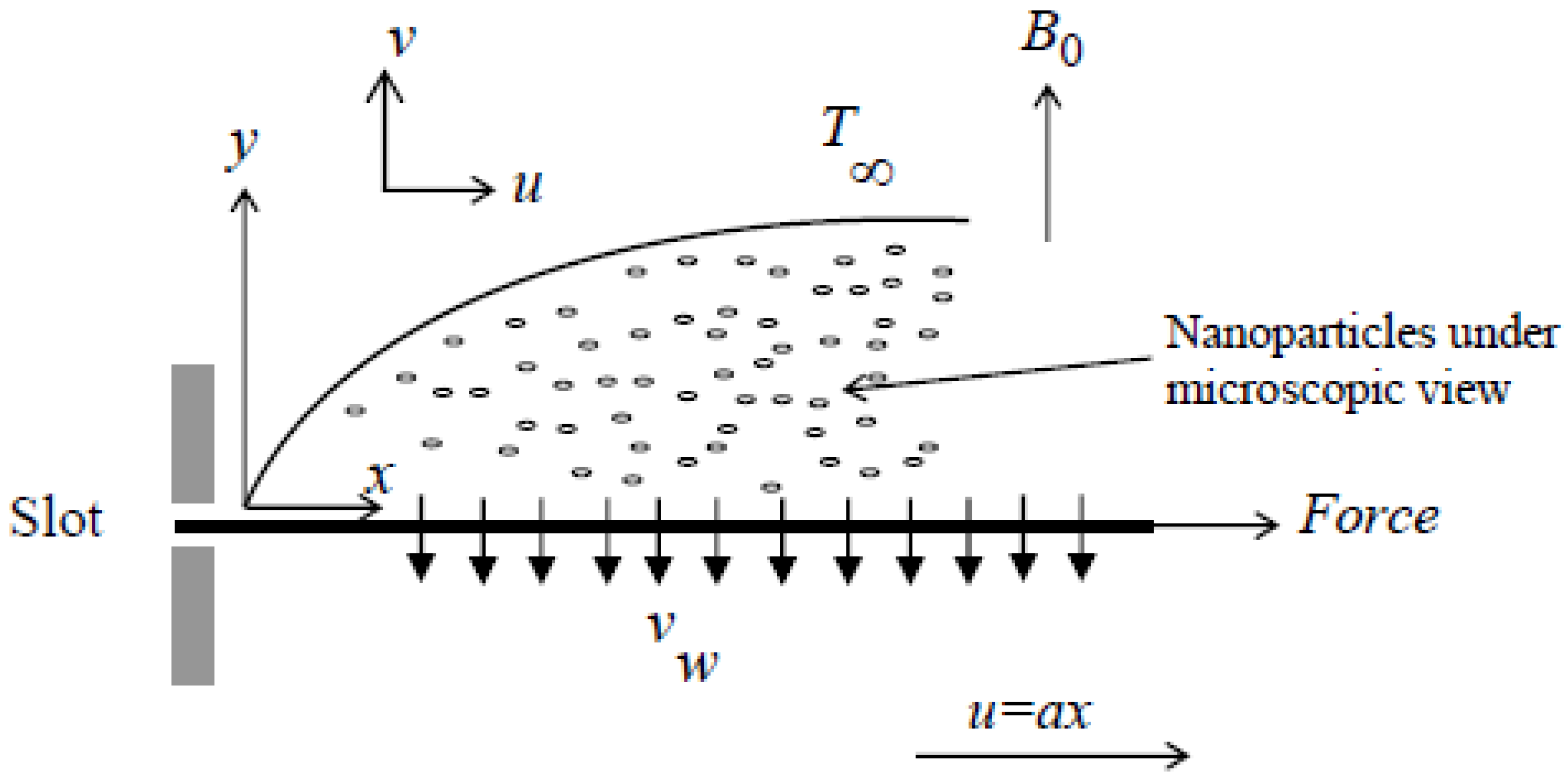
Consider an incompressible nanofluid flowing through a permeable stretched sheet in a boundary layer with effects from radiation, viscous dissipation and convective heating. The x-axis and y-axis are perpendicular to each other in the problem geometry, with the surface lying along the x-axis. Here, heat and mass transmission mechanisms are explained in terms of the Brownian and thermophoresis characteristics with diffusion coefficient $D_B$ and thermophoretic diffusion coefficient $D_T$, respectively. Additionally, the phenomenon of convective heat transfer is also taken into account. In the x-direction, the sheet is stretched with velocity $u_w=ax$, where a is a positive constant with dimension $s^{-1}$. Likewise, the nanofluid flow is assumed to have the velocity vector $\overrightarrow{U}$ with two components u and v, which can take the form:

$$\overrightarrow{U}=u\overrightarrow{i}+v\overrightarrow{j}.$$

(1)

In this investigation, we assume that a hot fluid exists beneath the stretching sheet’s bottom surface. By using a convection phenomenon, this hot fluid, which has a temperature of $T_f$, significantly contributes to warming the stretching sheet’s surface. So, the heat transfer coefficient $h_f$ is created as a result. This temperature $T_f$ is thought to be in the following form:

$$T_f=T_{\infty }+A{x}^2,$$

(2)

where $T_{\infty }$ refers to a constant ambient cold fluid temperature, A is constant. Here, we have that $T_f>T_{\infty }$ is the highest temperature in the system. Furthermore, the nanofluid concentration $C_w\left(x\right)$ is assumed to take the form:

$$C_w\left(x\right)=C_{\infty }+c{x}^2,$$

(3)

where $C_{\infty }$ stands for the nanofluid concentration away from the sheet and c is a constant. Additionally, it is anticipated that the vector of the applied magnetic field would permeate the Maxwell nanofluid with electrical conductivity $\sigma$, which can be considered to be as follows:

$$\overrightarrow{B}\left(x\right)=B_0\overrightarrow{j},$$

(4)

where $B_0$, as shown in Figure 1, is a factor that indicates the intensity of the magnetic field acting in the y-positive axis’s direction.

Further, we assume that the sheet is porous and the nanofluid moves through the holes at a constant speed $v_w$. In Cartesian coordinates, x and y, the fundamental steady equations for the conservation of mass, momentum, thermal energy and nanoparticles for nanofluids can be expressed as [18]:

$$\frac{\partial u}{\partial x}+\frac{\partial v}{\partial y}=0,$$

(5)

$$u\frac{\partial u}{\partial x}+v\frac{\partial u}{\partial y}=\frac{1}{{\rho }_{\infty }}\frac{\partial }{\partial y}\left(\mu \left(T\right)\frac{\partial u}{\partial y}\right)-{\beta }_1\left(u^2\frac{{\partial }^{2}u}{\partial x^2}+v^2\frac{{\partial }^{2}u}{\partial y^2}+2uv\frac{{\partial }^{2}u}{\partial x\partial y}\right)-\frac{\sigma B_0^2}{{\rho }_{\infty }}u,$$

(6)

$$\begin{array}{cc}\hfill u\frac{\partial T}{\partial x}+v\frac{\partial T}{\partial y}=\frac{1}{{\rho }_{\infty }{c}_p}\frac{\partial }{\partial y}\left(\kappa \left(T\right)\frac{\partial T}{\partial y}\right)+& \frac{1}{{\rho }_{\infty }{c}_p}\left(\mu \left(T\right){\left(\frac{\partial u}{\partial y}\right)}^2-{\rho }_{\infty }{\beta }_1\left(2uv\frac{\partial u}{\partial x}\frac{\partial u}{\partial y}+v^2{\left(\frac{\partial u}{\partial y}\right)}^2\right)\right)+\hfill \\ & \tau \left[D_B\frac{\partial C}{\partial y}\frac{\partial T}{\partial y}+\frac{D_T}{T_{\infty }}{\left(\frac{\partial T}{\partial y}\right)}^2\right]-\frac{1}{{\rho }_{\infty }{c}_p}\frac{\partial q_r}{\partial y},\hfill \end{array}$$

(7)

$$u\frac{\partial C}{\partial x}+v\frac{\partial C}{\partial y}=D_B\frac{{\partial }^{2}C}{\partial y^2}+\frac{D_T}{T_{\infty }}\frac{{\partial }^{2}T}{\partial y^2},$$

(8)

where, ${\beta }_1$ is the Maxwell coefficient, ${\rho }_{\infty }$ is the ambient nanofluid density, $\mu \left(T\right)$ is the nanofluid viscosity, T is the nanofluid’s Maxwell temperature and $\kappa$ is the nanofluid thermal conductivity. Here, we must remember that the Maxwell fluid class, characterized by the Maxwell coefficient ${\beta }_1$, is the most basic category of non-Newtonian fluids. The properties of the relaxation time can be accurately described by this model. Furthermore, we must point out that if ${\beta }_1=0$, our model can be reduced to a Newtonian model. Further, according to the Rosseland approximation, the radiative heat transfer $q_r$ is represented by the expression [19]:

$$q_r=-\frac{4{\sigma }^{*}}{3k^{*}}\frac{\partial T^4}{\partial y}.$$

(9)

The term $T^4$ in the last equation is used to denote the slight temperature variation in the fluid. The Taylor’s series about $T_{\infty }$ is used to expand the variable $T^4$ as a linear function. Consequently, disregarding the higher order terms produces the following [20]:

$$T^4\cong 4T_{\infty }^{3}T-3T_{\infty }^4.$$

(10)

In order to fully formulate the suggested problem, following is an introduction to the boundary conditions for the distributions of velocity, temperature and concentration [21]:

$$\begin{array}{cc}\hfill u=ax+\left(\frac{{\lambda }_1}{{\mu }_{\infty }}\right)& \left(\mu \left(T\right)\frac{\partial u}{\partial y}-{\rho }_{\infty }{\beta }_1(2uv\frac{\partial u}{\partial x}+v^2\frac{\partial u}{\partial y})\right),v=-v_w,\hfill \\ & -\kappa \left(T\right){\left(\frac{\partial T}{\partial y}\right)}_w=h_f\left(T_f-T_w\right),C=C_w\left(x\right)=C_{\infty }+c{x}^2,aty=0,\hfill \end{array}$$

(11)

$$u\to 0,T\to T_{\infty },C\to C_{\infty }\mathrm{as}y\to \infty ,$$

(12)

where ${\mu }_{\infty }$ is the ambient viscosity of the nanofluid and ${\lambda }_1$ is the slip velocity factor. We now begin with dimensionless variables that can transform partial differential equations into ordinary differential equations before creating the solution procedure [21]:

$$\eta ={\left(\frac{a}{{\nu }_{\infty }}\right)}^{\frac{1}{2}}y,u=ax{f}^{\prime }\left(\eta \right),v=-{\left(a{\nu }_{\infty }\right)}^{\frac{1}{2}}f\left(\eta \right),$$

(13)

$$\theta \left(\eta \right)=\frac{T-T_{\infty }}{T_f-T_{\infty }},\varphi \left(\eta \right)=\frac{C-C_{\infty }}{C_w-C_{\infty }},$$

(14)

where f is the non-dimensional stream function, $\theta$ is the non-dimensional fluid temperature, $\varphi$ is the dimensionless concentration and $\eta$ is the dimensionless similarity variable. Furthermore, we assume in this study that the dimensionless temperature impacts the nanofluid thermal conductivity $\kappa \left(T\right)$ as well as the nanofluid viscosity $\mu \left(T\right)$ according to these laws [22]:

$$\mu ={\mu }_{\infty }{e}^{-\alpha \theta },\kappa ={\kappa }_{\infty }(1+\epsilon \theta ),$$

(15)

where ${\kappa }_{\infty }$ is the thermal conductivity away from the sheet, $\epsilon$ is the factor of the thermal conductivity, $\alpha$ is the viscosity parameter, ${\mu }_{\infty }$ is a constant viscosity of the nanofluid at the ambient. Here, we must observe that $\kappa ={\kappa }_{\infty }$ when the nanofluid temperature T is equal to the ambient temperature $T_{\infty }$. Therefore, the thermal conductivity of the nanofluid varies with temperature along the thermal boundary layer before being constant at ambient. The governing ordinary differential equations with boundary conditions are written as follows when the aforementioned Equations (13) and (14) are introduced into the momentum, energy and concentration equations:

$$\left(f^{‴}-\alpha f^{″}{\theta }^{\prime }\right)e^{-\alpha \theta }+f{f}^{″}-f^{\prime 2}+\beta \left(2f{f}^{\prime }{f}^{″}-f^2{f}^{‴}\right)-M{f}^{\prime }=0,$$

(16)

$$\frac{1}{Pr}\left(\epsilon {\theta }^{\prime 2}+(1+R+\epsilon \theta ){\theta }^{″}\right)+f{\theta }^{\prime }-2\theta f^{\prime }+Nt{\theta }^{\prime 2}+Nb{\theta }^{\prime }{\varphi }^{\prime }+Ec{f}^{″}\left(e^{-\alpha \theta }{f}^{″}+\beta \left(2f{f}^{\prime 2}-f^2{f}^{″}\right)\right)=0,$$

(17)

$${\varphi }^{″}+PrLe\left(f{\varphi }^{\prime }-2\varphi f^{\prime }\right)+\frac{Nt}{Nb}{\theta }^{″}=0.$$

(18)

According to the following modified boundary condition:

$$\begin{array}{cc}\hfill f=f_w,f^{\prime }=1+& \lambda \left(e^{-\alpha \theta }{f}^{″}+\beta (2f{f}^{\prime 2}-f^2{f}^{″})\right),\varphi =1,\hfill \\ & {\theta }^{\prime }=-\delta \left(\frac{1-\theta }{1+R+\epsilon \theta }\right),at\eta =0,\hfill \end{array}$$

(19)

$$f^{\prime }\to 0,\theta \to 0,\varphi \to 0,\mathrm{as}\eta \to \infty .$$

(20)

Nevertheless, it is crucial to remember that the current non-Newtonian model can be converted into a Newtonian model if $\beta$ is missing from the previous system. In addition, the equations above include the following dimensionless quantities and parameters:

$$\beta =a{\beta }_1,M=\frac{\sigma B_0^2}{a{\rho }_{\infty }},\lambda ={\lambda }_1\sqrt{\frac{a}{{\nu }_{\infty }}},Nb=\frac{\tau D_B\left(C_w-C_{\infty }\right)}{{\nu }_{\infty }},Ec=\frac{a^2}{A{c}_p},$$

(21)

$$Nt=\frac{\tau D_T\left(T_f-T_{\infty }\right)}{{\nu }_{\infty }{T}_{\infty }},R=\frac{16{\sigma }^{*}{T}_{\infty }^3}{3{\kappa }_{\infty }{k}^{*}},\delta =\frac{h_f}{{\kappa }_{\infty }}\sqrt{\frac{{\nu }_{\infty }}{a}},Le=\frac{{\kappa }_{\infty }}{{\rho }_{\infty }{c}_p{D}_B},Pr=\frac{{\mu }_{\infty }{c}_p}{{\kappa }_{\infty }},$$

(22)

where $\beta$ is the Maxwell parameter and measures the relaxation time and $M,\lambda ,Nb,Ec$ are the magnetic number, slip velocity parameter, Brownian motion parameter and Eckert number, which denote the viscous dissipation phenomenon. $Nt$ is the thermophoresis parameter, R is the thermal radiation parameter and $\delta ,Le,Pr$ are the surface-convection parameter, Lewis parameter and Prandtl number, respectively.

Skin friction $C{f}_x$, heat transfer rate in term of $Nux$ and mass transfer rate in terms of $Shx$ are the physical characteristics of Maxwell nanofluid flow. These terms are denoted as follows:

$$\begin{array}{cc}\hfill & \frac{C{f}_x}{2}R{e}_x^{\frac{1}{2}}=-\left[e^{-\alpha \theta \left(0\right)}{f}^{″}\left(0\right)-\beta (f^{″}\left(0\right)f^2\left(0\right)-2f\left(0\right)f^{\prime 2}\left(0\right))\right],\hfill \\ & \frac{N{u}_x}{\sqrt{R{e}_x}}=-{\theta }^{\prime }\left(0\right),\frac{S{h}_x}{\sqrt{R{e}_x}}=-{\varphi }^{\prime }\left(0\right),\hfill \end{array}$$

(23)

where $R{e}_x=\frac{u_{w}x}{{\nu }_{\infty }}$ is the local Reynolds number.

3. Physical and Graphical Interpretation of Results

Here, a comprehensive investigation of radiative, MHD Maxwell nanofluid flow is described in this research using the shooting method, under the impact of slip velocity, viscous dissipation and convective heating phenomenon. Firstly, a comparison of numerical values representing the rate of heat transfer ($-{\theta }^{\prime }\left(0\right)$) for various suction parameters $f_w$ and the Prandtl number Pr with results previously published (Ishak et al. [23]) is presented in

Table 1. Comparison of Nusselt number $-{\theta }^{\prime }\left(0\right)$ for different values of $f_w$ and Pr with the results of Ishak et al. [23] when $\alpha =\beta =M=Ec=\lambda =R=\epsilon =Nt=Nb=0$.

Pr	${\mathit{f}}_{\mathit{w}}$,	Ishak et al. [23]	Present Work
0.72	−1.5	0.4570	0.457001520
1.0	−1.5	0.5000	0.500000000
10	−1.5	0.6542	0.654211910
0.72	0.0	0.8086	0.808589088
1.0	0.0	1.0000	1.000000000
3.0	0.0	1.9237	1.923689985
10.0	0.0	3.7207	3.720699510
0.72	1.5	1.4944	1.494389791
1.0	1.5	2.0000	2.000002010
10	1.5	16.0842	16.08419892

as evidence of the reliability of the existing solutions.

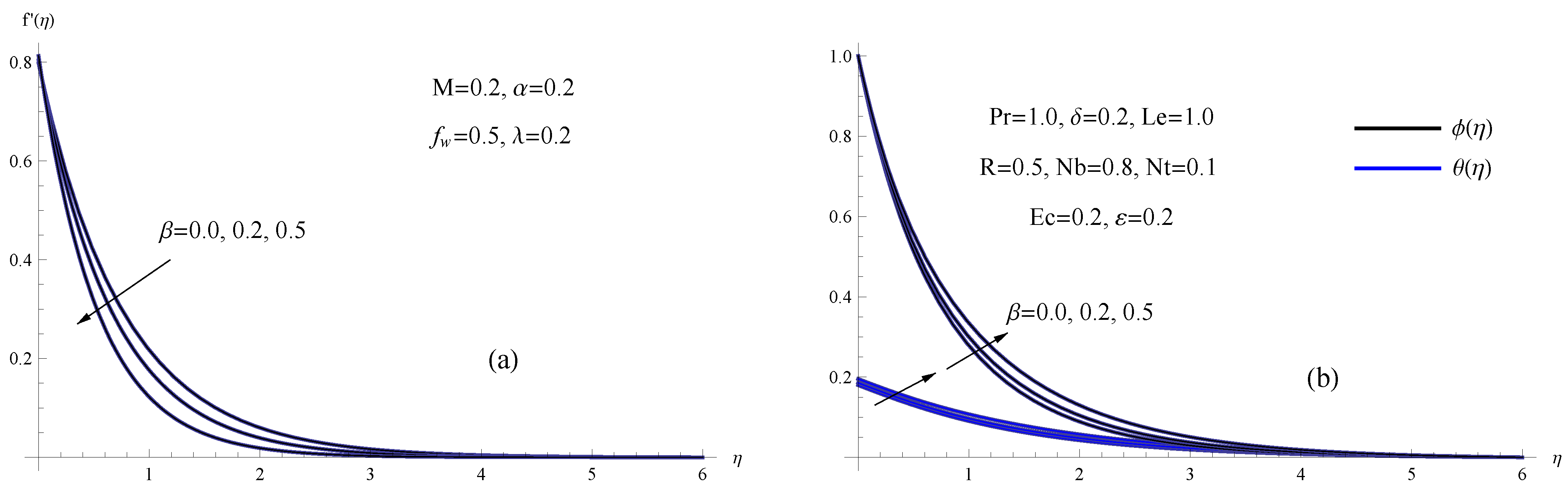
Figure 2 shows three different values of the Maxwell parameter side-by-side comparisons of the fields of velocity, temperature and concentration. As can be seen, Figure 2 depicts a significant resistance to flow velocity with increasing Maxwell parameter values due to the development of shear stress. Additionally, the temperature of the sheet $\theta \left(0\right)$ as well as the temperature $\theta \left(\eta \right)$ and concentration $\varphi \left(\eta \right)$ distributions were all dramatically increased by the same parameter.

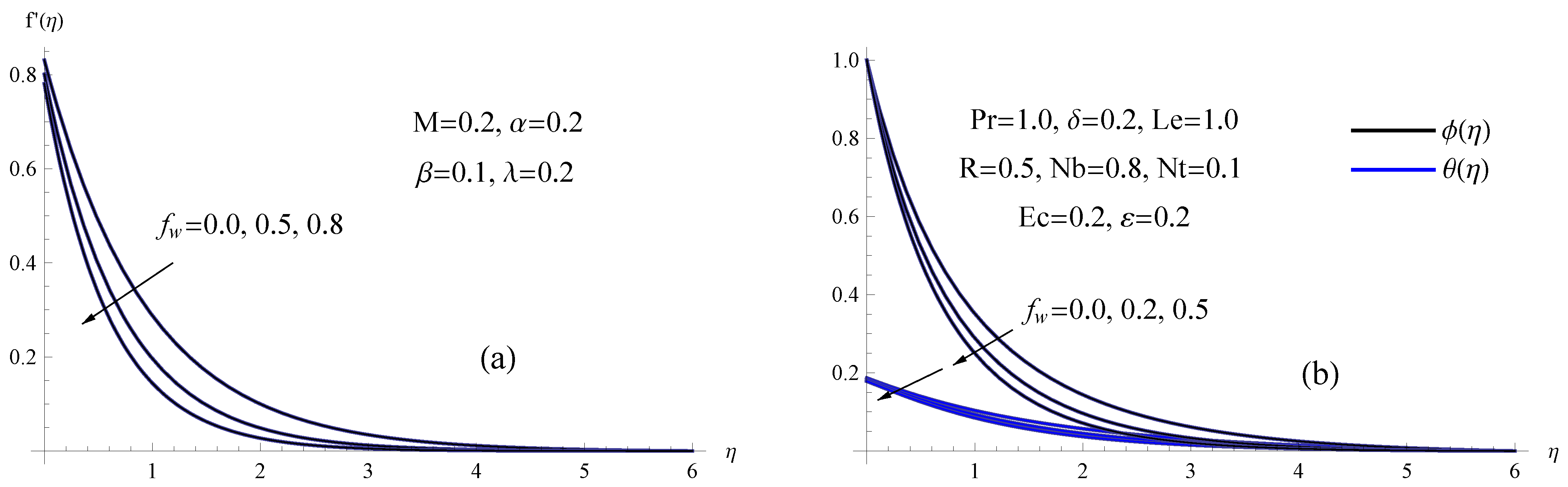
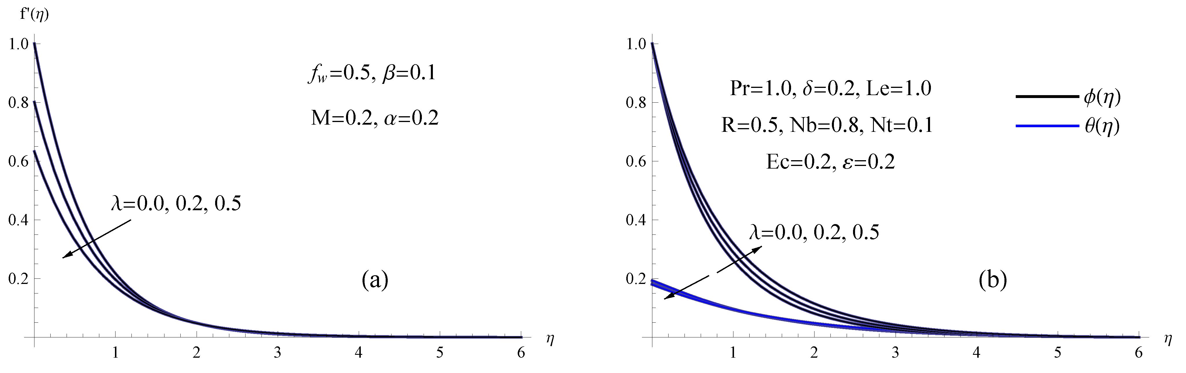
According to the change of the suction parameter $f_w$, Figure 3 shows the analysis of the flow and heat mass transportation performance of Maxwell nanofluid. An intriguing finding is that the classical model specifies the lowest fluid flow for high values of the suction parameter while having the fastest velocity profile for low values. Higher suction parameter values lessen the mass distribution while enhancing the cooling of the nanofluid and the sheet temperature $\theta \left(0\right)$ since the fluid displays the fastest heat and mass transfer in the absence of the suction parameter (impermeable sheet).

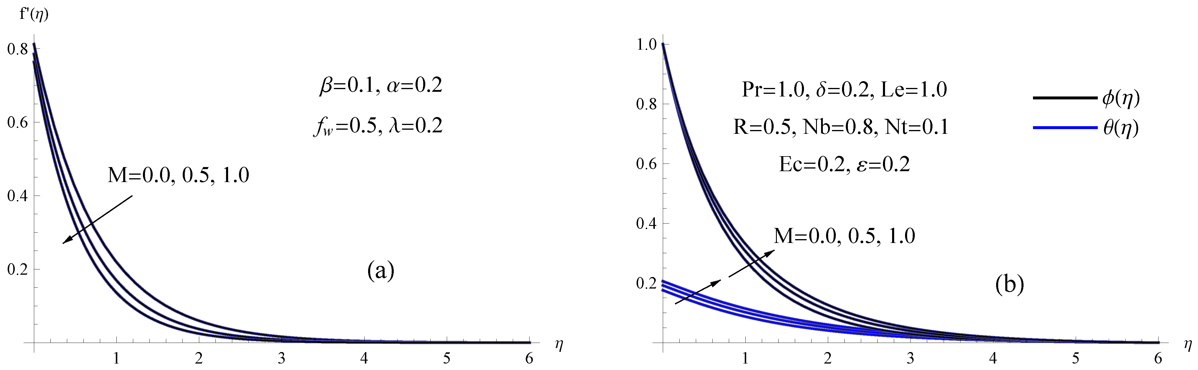
Figure 4 depicts variations in velocity $f^{\prime }\left(\eta \right)$, temperature $\theta \left(\eta \right)$ and concentration $\varphi \left(\eta \right)$ caused by the magnetic field’s M impact on the Maxwell nanofluid. Various inputs of the non-dimensional magnetic parameter M are used in this investigation while holding the inputs of other related physical parameters constant. The velocity of the nanofluid is observed to be restricted by an increase in the magnetic parameter. The existence of the Lorentz force is the physical component that causes this result. One of the viscous forces of this type, the Lorentz force, works in the opposite direction of nanofluid flow and slows down the fluid velocity. As a result, the creation of these viscous forces has a profound impact and causes the fluid to be warmed and concentrated to enhance the magnetic parameter.

For various values of the viscosity parameter $\alpha$, Figure 5 explains the demeanor of the velocity $f^{\prime }\left(\eta \right)$, temperature $\theta \left(\eta \right)$ and concentration $\varphi \left(\eta \right)$ fields. The graphic shows that as the viscosity parameter climbs, the momentum boundary layer thickness and velocity field slow down. The essential duty of nanofluid viscosity, which mostly depends on temperature, is to promote mass and heat transfer rates within the boundary layer. As a result, it is evident that as the viscosity parameter improves, the concentration and temperature of nanofluid as well as the sheet temperature $\theta \left(0\right)$ and the thickness of the thermal boundary layer rise. Clearly the velocity distribution through the boundary layer was greatly impacted by the viscosity parameter $\alpha$ since the viscosity parameter directly influences the velocity field, as seen from Equation (16). While the concentration and temperature fields are both indirectly influenced by the viscosity parameter, and as a result, both are only marginally impacted.

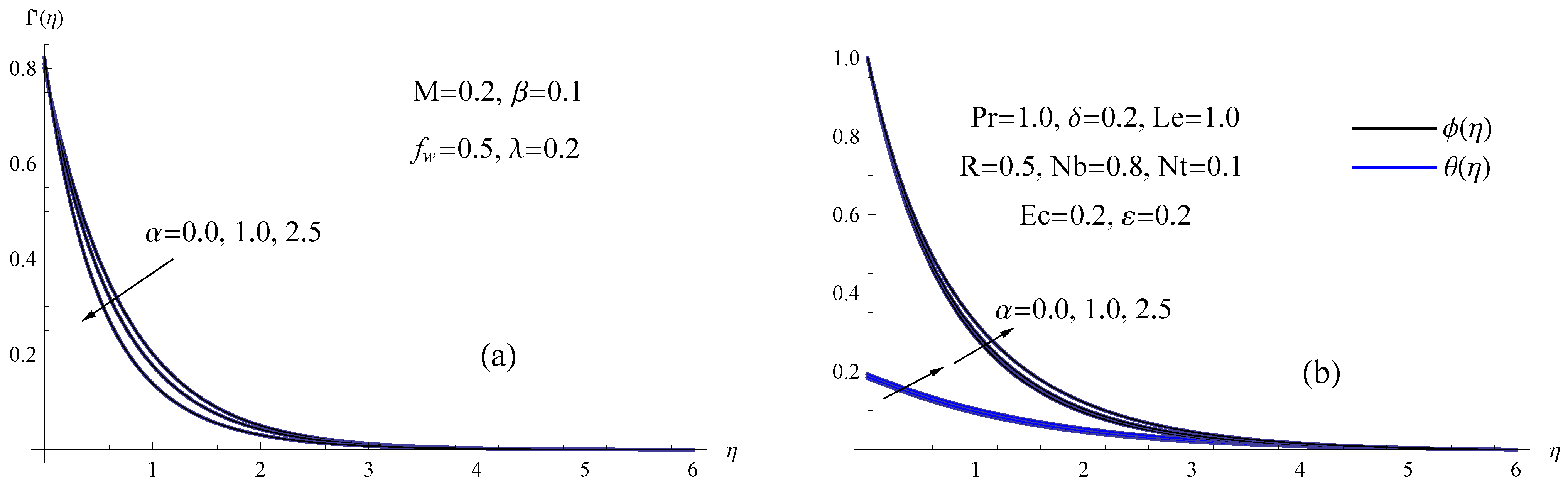
Figure 6 examines the impact of the slip velocity parameter $\lambda$ on the velocity $f^{\prime }\left(\eta \right)$, temperature $\theta \left(\eta \right)$ and concentration $\varphi \left(\eta \right)$ fields while the other physical governing parameters are unchanged. We notice that anytime the slip velocity $\lambda$ increases, both the sheet velocity $f^{\prime }\left(0\right)$ and the nanofluid velocity $f^{\prime }\left(\eta \right)$ dramatically decrease with the dimensionless variable $\eta$. Additionally, we see that the velocity distribution changes as $\eta$ is increased in the interval $0\le \lambda <2$. Further, when the slip velocity parameter $\lambda$ improves, the same drop tendency is shown for both the temperature distribution $\theta \left(\eta \right)$ and the sheet temperature $\theta \left(0\right)$. Moreover, we can see from the following graphic that with rising values of $\lambda$, the boundary layer thickness and the concentration field both get better.

According to the influence of the Eckert number $Ec$, the temperature distribution $\theta \left(\eta \right)$ shows modification in Figure 7a. In the nanofluid heat transfer mechanism, the principal objective of the viscous dissipation phenomena is to alter the thermal performance with sources of energy. Larger Eckert number values indicate that heat is dissipating and traveling in the direction of the fluid as a result of viscous force. Fluid particles travel quickly as a result, causing more collisions between them. This greater collision produces thermal energy by converting kinetic energy. Furthermore, the graph of the temperature field $\theta \left(\eta \right)$ for miscellaneous values of thermal radiation parameter R is designed in Figure 7b. With the higher thermal radiation parameter along the sheet, as opposed to away from it, a significant drop in both the sheet temperature $\theta \left(0\right)$ and the nanofluid temperature is seen.

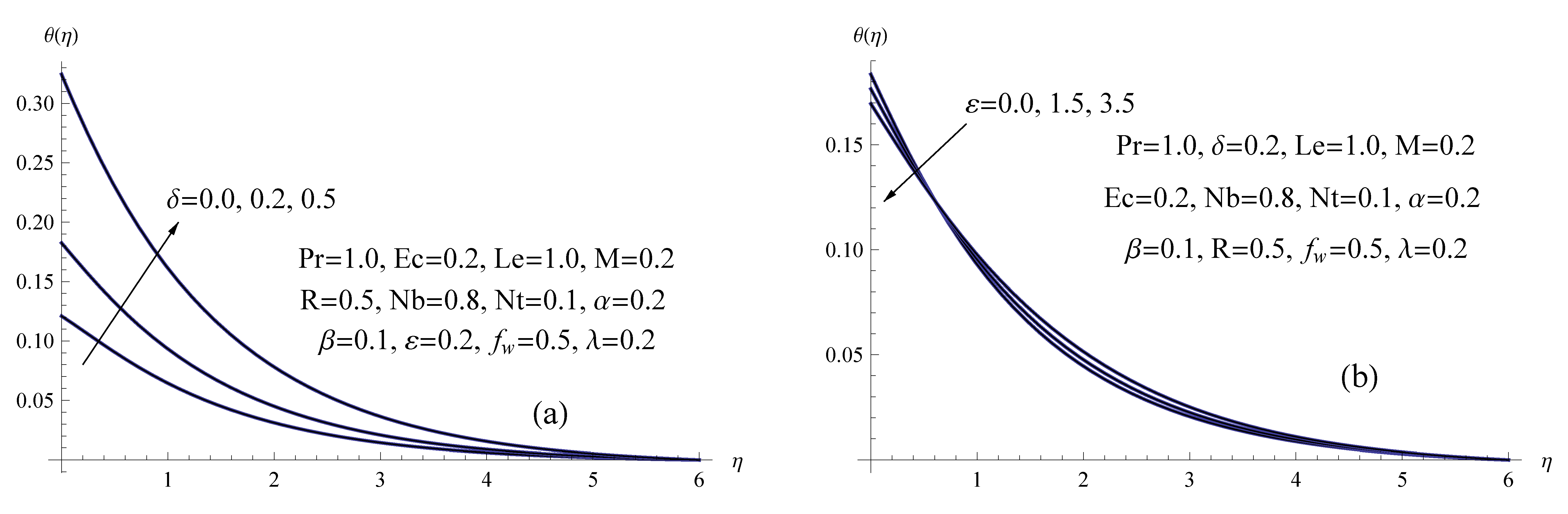
Figure 8 shows how the surface-convection parameter $\delta$ affects the temperature distributions $\theta \left(\eta \right)$ in the region of the thermal boundary layer. The nanofluid temperature $\theta \left(\eta \right)$ is seen to dramatically increase along the sheet wall but only modestly rise away from the sheet, especially when $\eta$ is greater than 4.0. As a result, the nanofluid along the sheet warmed due to higher values of the surface-convection parameter, which thickened the thermal boundary layer. Figure 8b illustrates the graphical behavior of the nanofluid’s dimensionless temperature for various values of the thermal conductivity parameter $\epsilon$. It is evident that as $\epsilon$ increases, the Maxwell nanofluid temperature and the thermal boundary layer thickness grow away from the sheet wall, whereas the reverse trend is noted beside the sheet. In contrast to nanofluids with constant thermal conductivity, this causes the thermal boundary layer thickness of the nanofluid with variable thermal conductivity to be greater.

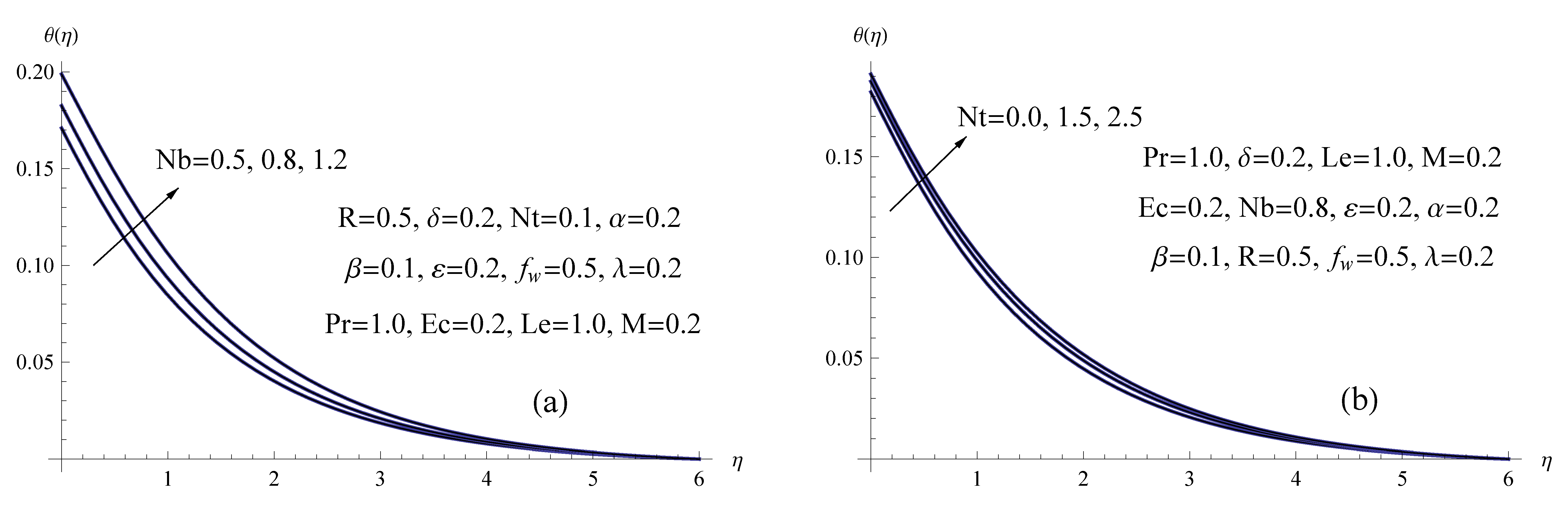
Additionally, Figure 9 shows the temperature field $\theta \left(\eta \right)$ outcomes for the Brownian motion parameter $Nb$ and the thermophoresis parameter $Nt$. The particles’ erratic motion generates extra kinetic energy, which boosts the thermal energy that is already there. As a result, a rise in $Nb$ causes the fluid temperature in the boundary layer’s thermal domain to increase faster. The Maxwell nanofluid temperature and the sheet temperature $\theta \left(0\right)$ both accelerated similarly as a result of the increase in the thermophoresis parameter $Nt$.

Before we have finished our analysis, we must concentrate on the drag force, which can be calculated using the skin-friction coefficient $\frac{C{f}_x}{2}R{e}_x^{\frac{1}{2}}$, rate of heat transfer (which can be evaluated using the local Nusselt number $\frac{N{u}_x}{\sqrt{R{e}_x}}$), and the rate of mass transfer, which can be determined using the local Sherwood number $\frac{S{h}_x}{\sqrt{R{e}_x}}$. Therefore, we are interested to examine the key physical characteristics that can influence how these quantities behave. In order to obtain these values for this work, we constructed

Table 2. Values of $\frac{C{f}_x}{2}R{e}_x^{\frac{1}{2}}$, $\frac{N{u}_x}{\sqrt{R{e}_x}}$ and $\frac{S{h}_x}{\sqrt{R{e}_x}}$ for various values of $\beta ,f_w,M,\alpha ,\lambda ,Ec,R,\delta$ and $\epsilon$ with $Nb=0.8,Le=1.0,Pr=1.0$ and $Nt=0.1$.

$\mathit{\beta }$	${\mathit{f}}_{\mathit{w}}$	M	$\mathit{\alpha }$	$\mathit{\lambda }$	$\mathit{Ec}$	R	$\mathit{\delta }$	$\mathit{\epsilon }$	$\frac{{\mathit{Cf}}_{\mathit{x}}}{2}{\mathit{Re}}_{\mathit{x}}^{\frac{1}{2}}$	$\frac{{\mathit{Nu}}_{\mathit{x}}}{\sqrt{{\mathit{Re}}_{\mathit{x}}}}$	$\frac{{\mathit{Sh}}_{\mathit{x}}}{\sqrt{{\mathit{Re}}_{\mathit{x}}}}$
0.0	0.5	0.2	0.2	0.2	0.2	0.5	0.2	0.2	1.010101	0.106808	1.404140
0.2	0.5	0.2	0.2	0.2	0.2	0.5	0.2	0.2	0.980241	0.105987	1.361981
0.5	0.5	0.2	0.2	0.2	0.2	0.5	0.2	0.2	0.937128	0.104581	1.291542
0.1	0.0	0.2	0.2	0.2	0.2	0.5	0.2	0.2	0.845444	0.105775	1.168950
0.1	0.5	0.2	0.2	0.2	0.2	0.5	0.2	0.2	0.995036	0.106410	1.383612
0.1	0.8	0.2	0.2	0.2	0.2	0.5	0.2	0.2	1.095980	0.106979	1.536251
0.1	0.5	0.0	0.2	0.2	0.2	0.5	0.2	0.2	0.937012	0.107398	1.414660
0.1	0.5	0.5	0.2	0.2	0.2	0.5	0.2	0.2	1.071621	0.105056	1.342411
0.1	0.5	1.0	0.2	0.2	0.2	0.5	0.2	0.2	1.179310	0.103068	1.284550
0.1	0.5	0.2	0.0	0.2	0.2	0.5	0.2	0.2	1.003950	0.106514	1.388790
0.1	0.5	0.2	1.0	0.2	0.2	0.5	0.2	0.2	0.958801	0.105961	1.360981
0.1	0.5	0.2	2.5	0.2	0.2	0.5	0.2	0.2	0.888192	0.104945	1.308652
0.1	0.5	0.2	0.2	0.0	0.2	0.5	0.2	0.2	1.329681	0.104874	1.515341
0.1	0.5	0.2	0.2	0.2	0.2	0.5	0.2	0.2	0.995036	0.106410	1.383612
0.1	0.5	0.2	0.2	0.5	0.2	0.5	0.2	0.2	0.734743	0.106767	1.258561
0.1	0.5	0.2	0.2	0.2	0.0	0.5	0.2	0.2	0.997361	0.112547	1.383421
0.1	0.5	0.2	0.2	0.2	0.2	0.5	0.2	0.2	0.995036	0.106410	1.383612
0.1	0.5	0.2	0.2	0.2	0.5	0.5	0.2	0.2	0.991547	0.097316	1.383845
0.1	0.5	0.2	0.2	0.2	0.2	0.0	0.2	0.2	0.994306	0.152219	1.379111
0.1	0.5	0.2	0.2	0.2	0.2	0.5	0.2	0.2	0.995036	0.106410	1.383612
0.1	0.5	0.2	0.2	0.2	0.2	1.0	0.2	0.2	0.995541	0.081922	1.386090
0.1	0.5	0.2	0.2	0.2	0.2	0.5	0.0	0.2	0.997938	0.057677	1.389350
0.1	0.5	0.2	0.2	0.2	0.2	0.5	0.2	0.2	0.995036	0.106410	1.383612
0.1	0.5	0.2	0.2	0.2	0.2	0.5	0.5	0.2	0.988322	0.215834	1.370541
0.1	0.5	0.2	0.2	0.2	0.2	0.5	0.2	0.0	0.995008	0.108859	1.383361
0.1	0.5	0.2	0.2	0.2	0.2	0.5	0.2	1.5	0.995196	0.093315	1.384910
0.1	0.5	0.2	0.2	0.2	0.2	0.5	0.2	3.5	0.995396	0.079346	1.386282

. It is evident from Table 2 that as the Maxwell number, viscosity parameter, slip velocity parameter and surface-convection parameter grow, the local skin-friction coefficient changes inversely. Additionally, a reduction in the Sherwood number is brought about by rising values of the Maxwell number, magnetic number, viscosity parameter and slip velocity parameter, whereas the remaining parameters affect the Sherwood number in the opposite direction. In addition, increasing the suction, slip and surface-convection parameters elevates the values of the local Nusselt number, but the opposite trend is shown for the remaining parameters. Last but not least, the thermal conductivity parameter can increase the local Sherwood number and the skin friction coefficient values while having an opposite impact on the Nusselt number.

4. Conclusions

Maxwell nanofluid flow caused by stretching surfaces has presented numerous challenges to the fluid mechanics research community as a result of widespread applications in the commercial and industrial sectors. As a result, the main goal of this work is to elucidate how the convective heating and viscous dissipation phenomena, which are connected to the variable thermo-physical properties, affect the slippery flow of the Maxwell MHD nanofluid toward a stretching horizontal sheet. The simplified reduced core governing equations are numerically solved using the shooting method. Graphs and tables are used to investigate how physical parameters affect fluctuations in velocity, temperature, concentration, skin-friction coefficient, Sherwood number and the Nusselt number. The following findings are achieved after computation and observation.

• The increased Maxwell parameter, slip velocity parameter, viscosity parameter, magnetic number and suction parameter diminishes the nanofluid velocity.
• Eckert number and surface-convection parameter values that are larger result in magnifying values for the temperature field.
• The suction parameter, thermal conductivity parameter and magnetic parameter all raise the skin-friction coefficient.
• The results showed that the existence of thermophoresis and Brownian motion makes the heat transmission phenomena more effective.
• Higher radiation and suction parameter values result in a larger Sherwood number, while Maxwell and slip velocity parameter values result in a smaller Sherwood number.
• A larger magnetic number, Brownian motion parameter, viscosity parameter and Maxwell parameter will result in a temperature rise whereas a higher suction parameter and slip velocity parameter will reduce the temperature.
• The concentration of the nanofluid is severely degraded as the viscosity, magnetic number, Maxwell and slip velocity parameters drop.

References

- Choi, S.U.S. Enhancing thermal conductivity of fluids with nanoparticles. ASME FED 1995, 231, 99–103. [Google Scholar]
- Yu, W.; France, D.M.; Routbort, J.L.; Choi, S.U.S. Review and comparison of nanofluid thermal conductivity and heat transfer enhancements. Heat Transf. Eng. 2008, 29, 432–460. [Google Scholar] [CrossRef]
- Buongiorno, J. Convective transport in nanofluids. ASME J. Heat Mass Transf. 2006, 128, 240–250. [Google Scholar] [CrossRef]
- Awais, M.; Hayat, T.; Irum, S.; Alsaedi, A. Heat generation/absorption effects in a boundary layer stretched flow of Maxwell nanofluid; Analytic and Numeric solutions. PLoS ONE 2015, 10, e0129814. [Google Scholar] [CrossRef]
- Shafique, Z.; Mustafa, M.; Mushtaq, A. Boundary layer flow of Maxwell fluid in rotating frame with binary chemical reaction and activation energy. Res. Phys. 2016, 6, 627–633. [Google Scholar] [CrossRef] [Green Version]
- Hayat, T.; Khan, M.I.; Waqas, M.; Alsaedi, A.; Khan, M.I. Radiative flow of micropolar nanofluid accounting thermophoresis and Brownian moment. Int. J. Hydrogen Energy 2017, 42, 16821–16833. [Google Scholar] [CrossRef]
- Sharma, K.; Gupta, S. Viscous dissipation and thermal radiation effects in MHD flow of Jeffrey nanofluid through impermeable surface with heat generation/absorption. Nonlinear Eng. 2017, 6, 153–166. [Google Scholar] [CrossRef]
- Patel, H.R.; Mittal, A.S.; Darji, R.R. MHD flow of micropolar nanofluid over a stretching/shrinking sheet considering radiation. Int. Commun. Heat Mass Transf. 2019, 108, 104322. [Google Scholar] [CrossRef]
- Noor, N.A.M.; Shafie, S.; Admon, M.A. Slip effects on MHD squeezing flow of Jeffrey nanofluid in horizontal channel with chemical reaction. Mathematics 2021, 9, 1215. [Google Scholar] [CrossRef]
- Mangathai, P.; Reddy, B.R.; Sidhartha, C. Unsteady MHD Williamson and Casson nanofluid flow in the presence of radiation and viscous dissipation. Turk. J. Comput. Math. Educ. 2021, 12, 1036–1051. [Google Scholar]
- Alotaibi, H.; Althubiti, S.; Eid, M.R.; Mahny, K.L. Numerical treatment of MHD flow of Casson nanofluid via convectively heated non-linear extending surface with viscous dissipation and suction/injection effects. Comput. Mater. Contin. 2021, 66, 229–245. [Google Scholar] [CrossRef]
- Sheikholeslami, M.; Abelman, S.; Ganji, D.D. Numerical simulation of MHD nanofluid flow and heat transfer considering viscous dissipation. Int. J. Heat Mass Transf. 2014, 79, 212–222. [Google Scholar] [CrossRef]
- Hussain, S. Finite element solution for MHD flow of nanofluids with heat and mass transfer through a porous media with thermal radiation, viscous dissipation and chemical reaction effects. Adv. Appl. Math. Mech. 2017, 9, 904–923. [Google Scholar] [CrossRef]
- Ibrahim, W.; Negera, M. Viscous dissipation effect on Williamson nanofluid over stretching/shrinking wedge with thermal radiation and chemical reaction. J. Phys. Commun. 2020, 4, 045015. [Google Scholar] [CrossRef]
- Lund, L.A.; Omar, Z.; Khan, I.; Raza, J.; Sherif, E.M.; Seikh, A.H. Magnetohydrodynamic (MHD) flow of micropolar fluid with effects of viscous dissipation and joule heating over an exponential shrinking sheet: Triple solutions and stability analysis. Symmetry 2020, 12, 142. [Google Scholar] [CrossRef] [Green Version]
- Saadi, F.A.; Worthy, A.; Alrihieli, H.; Nelson, M. Localised spatial structures in the Thomas model. Math. Comput. Simul. 2022, 194, 141–158. [Google Scholar] [CrossRef]
- Li, X.; Alrihieli, H.; Algehyne, E.A.; Khan, M.A.; Alshahrani, M.Y.; Alraey, Y.; BilalRiaze, M. Application of piecewise fractional differential equation to COVID-19 infection dynamics. Results Phys. 2022, 39, 105685. [Google Scholar] [CrossRef]
- Ramzan, M.; Bilal, M.; Chung, J.D.; Farooq, U. Mixed convective flow of Maxwell nanofluid past a porous vertical stretched surface—An optimal solution. Results Phys. 2016, 6, 1072–1079. [Google Scholar] [CrossRef] [Green Version]
- Bardos, C.; Golse, F.; Perthame, B. The Rosseland approximation for the radiative transfer equations. Commun. Pure Appl. Math. 1987, 40, 691–721. [Google Scholar] [CrossRef]
- Algehyne, E.A.; Alrihieli, H.; Saeed, A.; Alduais, F.S.; Hayat, A.U.; Kumam, P. Numerical simulation of 3D Darcy & Forchheimer fluid flow with the energy and mass transfer over an irregular permeable surface. Sci. Rep. 2022, 12, 14629. [Google Scholar]
- Megahed, A.M. Improvement of heat transfer mechanism through a Maxwell fluid flow over a stretching sheet embedded in a porous medium and convectively heated. Math. Comput. Simul. 2021, 187, 97–109. [Google Scholar] [CrossRef]
- Megahed, A.M.; Reddy, M.G.; Abbas, W. Modeling of MHD fluid flow over an unsteady stretching sheet with thermal radiation, variable fluid properties and heat flux. Math. Comput. Simul. 2021, 185, 583–593. [Google Scholar] [CrossRef]
- Ishak, A.; Nazar, R.; Pop, I. Heat transfer over an unsteady stretching permeable surface with prescribed wall temperature. Nonlinear Anal. Real World Appl. 2009, 10, 2909–2913. [Google Scholar] [CrossRef]
Figure 1.
Schematic diagram for the nanofluid flow.
Figure 2.
(a) The for chosen , (b) and for chosen .
Figure 3.
Figure 4.
(a) The for chosen M, (b) and for chosen M.
Figure 5.
Figure 6.
Figure 7.
(a) for chosen (b) for chosen R.
Figure 8.
(a) The for chosen , (b) for chosen .
Figure 9.