
Closed-Form Solution for the Natural Frequencies of Low-Speed Cracked Euler–Bernoulli Rotating Beams

Abstract
:1. Introduction
2. Mathematical Model and Formulation of the Problem
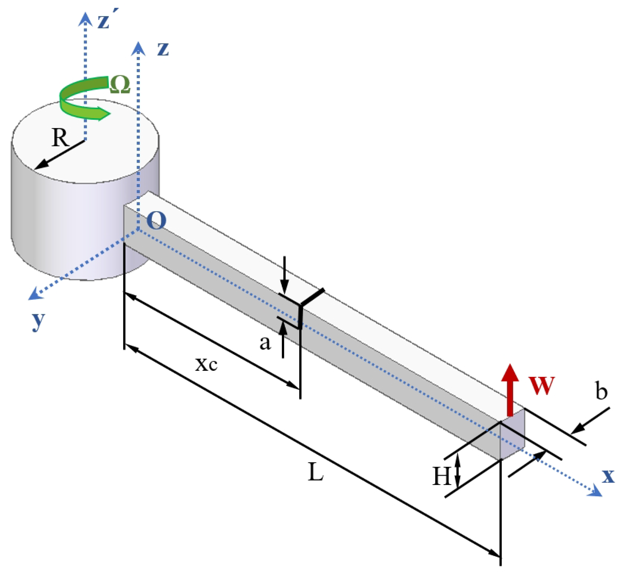
2.1. Model of the Cracked Euler–Bernoulli Rotating Beam
2.2. Solving the Equation of Motion
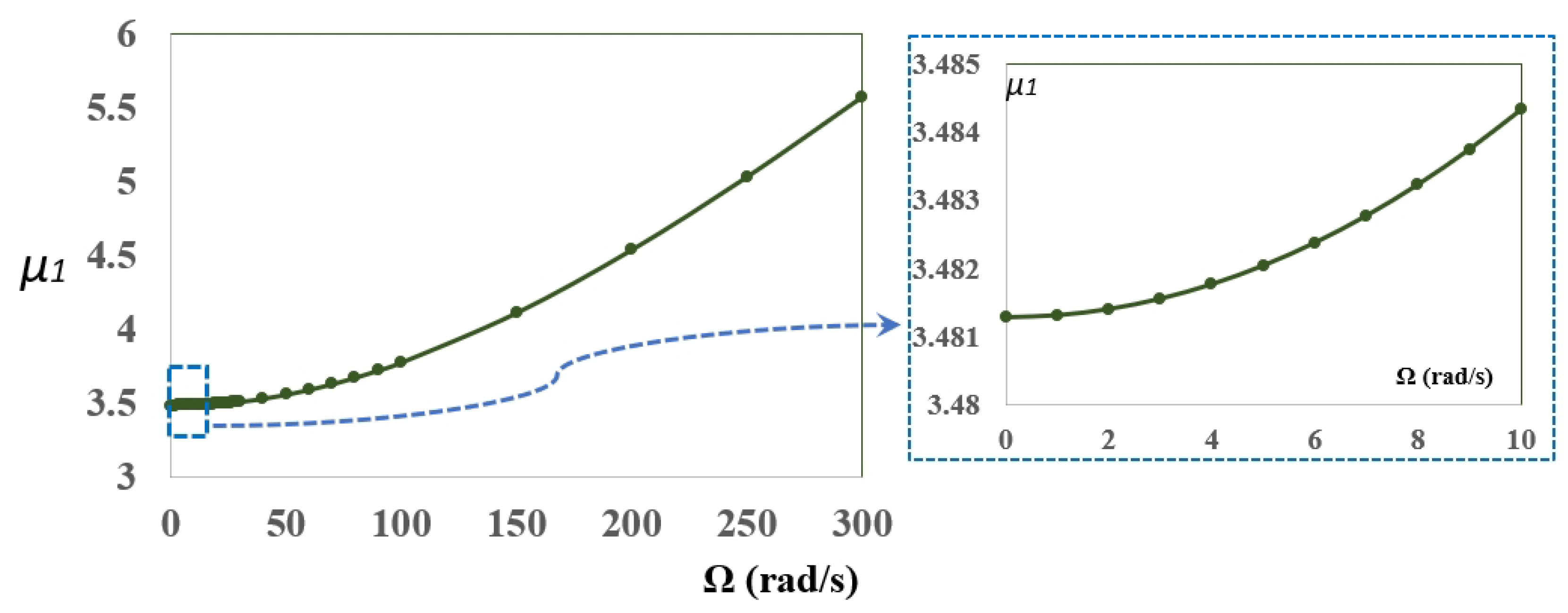
2.3. Verification of the Analytical Model
3. Determination of the Closed-Form Solutions
- Slenderness ratio: and 220, according to (18)
- Dimensionless hub radius: and ;
- Dimensionless crack location: and ;
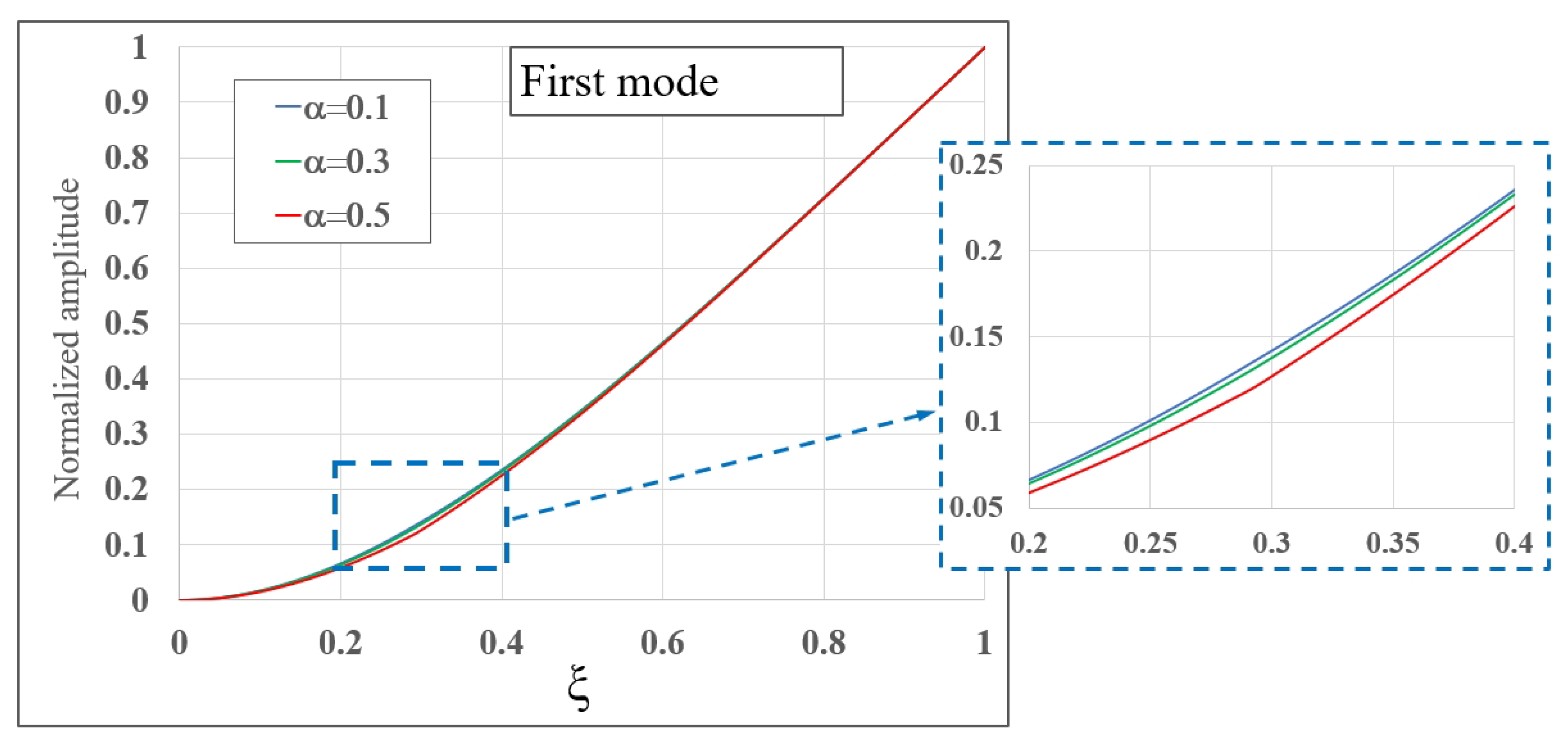
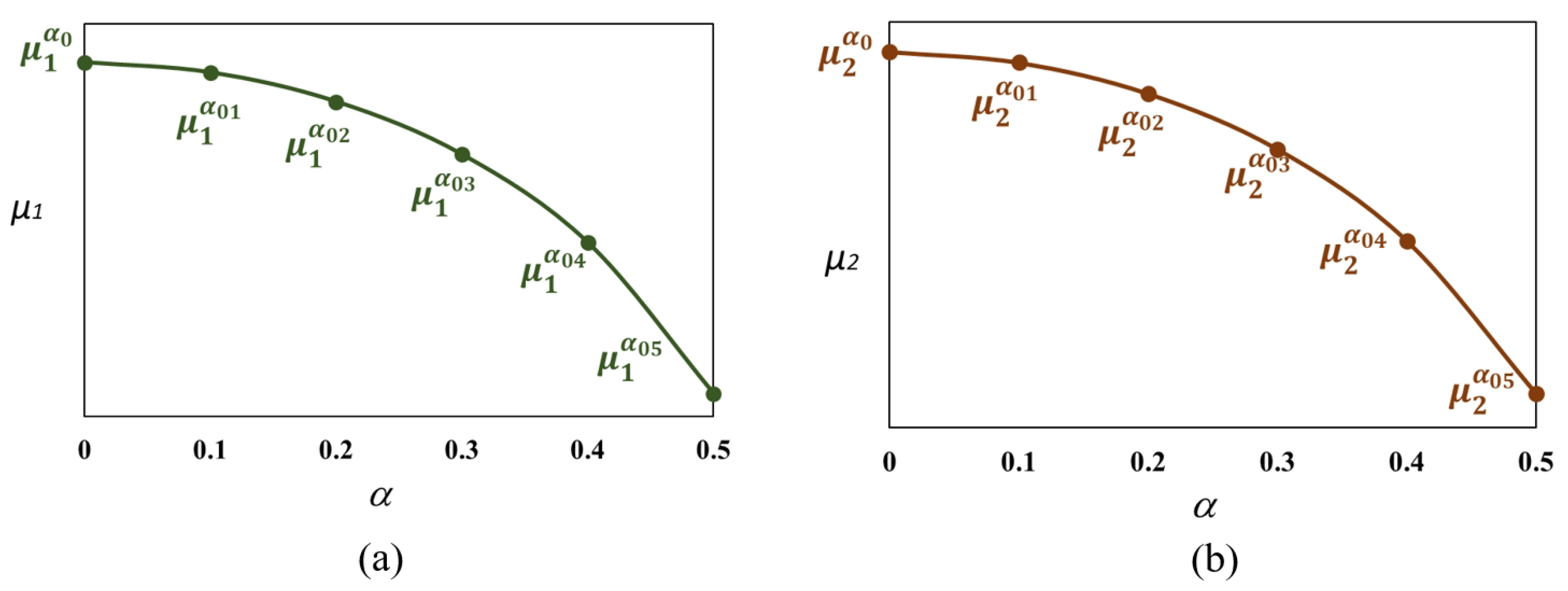
- Dimensionless crack depth: and , where corresponds to a healthy beam.
4. Reliability of the Closed-Form Solutions
5. Application of the Model, Discussion and Results
- rad/s
- and
- and
- rad/s
- and
- and
6. Conclusions
Author Contributions
Funding
Institutional Review Board Statement
Informed Consent Statement
Data Availability Statement
Conflicts of Interest
References
- Jackson, D.R. Dynamic stiffness matrix method for the free vibration analysis of rotating uniform shear beams. Proc. ASME Des. Eng. Tech. Conf. 2009, 1, 1315–1324. [Google Scholar]
- Bazoune, A. Survey on Modal Frequencies of Centrifugally Stiffened Beams. Shock Vib. Dig. 2005, 37, 449–469. [Google Scholar] [CrossRef]
- Kim, H.; Yoo, H.H.; Chung, J. Dynamic model for free vibration and response analysis of rotating beams. J. Sound Vib. 2013, 332, 5917–5928. [Google Scholar] [CrossRef]
- Banerjee, J.R. Dynamic stiffness formulation and free vibration analysis of centrifugally stiffened Timoshenko beams. Comput. Struct. 2001, 247, 97–115. [Google Scholar] [CrossRef]
- Bazoune, A.; Khulief, Y.A.; Stephen, N.G. Further results for modal characteristics of rotating tapered Timoshenko beams. J. Sound Vib. 1999, 219, 157–174. [Google Scholar] [CrossRef] [Green Version]
- Ozgumus, O.O.; Kaya, M.O. Vibration analysis of a rotating tapered Timoshenko beam using DTM. Meccanica 2010, 45, 33–42. [Google Scholar] [CrossRef]
- Mishnaevsky, L.; Branner, K.; Nørgaard Petersen, H.; Beauson, J.; McGugan, M.; Sørensen, F. Materials for Wind Turbine Blades: An Overview. Materials 2017, 10, 1285. [Google Scholar] [CrossRef] [Green Version]
- Zhu, M. Design and analysis of steam turbine blades. IOP Conf. Ser. J. Phys. Conf. Ser. 2019, 1300, 012056. [Google Scholar] [CrossRef] [Green Version]
- Lee, J.W.; Lee, J.Y. In-plane bending vibration analysis of a rotating beamwith multiple edge cracks by using the transfer matrix method. Meccanica 2017, 52, 1143–1157. [Google Scholar] [CrossRef]
- Hsu, T.Y.; Shiao, S.Y.; Liao, W.I. Damage detection of rotating wind turbine blades using local flexibility method and long-gauge fiber Bragg grating sensors. Meas. Sci. Technol. 2018, 29, 015108. [Google Scholar] [CrossRef]
- Fang, J.; Zhou, D.; Dong, Y. Effect of cracks on nonlinear flexural vibration of rotating Timoshenko functionally graded material beam having large amplitude motion. Proc. Inst. Mech. Eng. Part C J. Mech. Eng. Sci. 2019, 232, 930–940. [Google Scholar]
- Fang, J.; Zhou, D.; Dong, Y. Three-dimensional vibration of rotating functionally graded beams. J. Vib. Control 2018, 24, 3292–3306. [Google Scholar] [CrossRef]
- Fang, J.; Zhou, D. In-Plane Vibration Analysis of Rotating Tapered Timoshenko Beams. Int. J. Appl. Mech. 2016, 8, 1650064. [Google Scholar] [CrossRef]
- Bhat, R.B. Transverse vibrations of a rotating uniform cantilever beam with tip mass as predicted by using beam characteristic orthogonal polynomials in the Rayleigh–Ritz Method. J. Sound Vib. 1896, 105, 199–210. [Google Scholar] [CrossRef]
- Yoo, H.H.; Cho, J.E.; Chung, J. Modal analysis at shape optimization of rotating cantilever beams. J. Sound Vib. 2006, 290, 223–241. [Google Scholar] [CrossRef]
- Mazanoglu, K.; Guler, S. Flap-wise and chord-wise vibrations of axially functionally grades tapered beams rotating around a hub. Mech. Syst. Signal Process 2017, 89, 97–107. [Google Scholar] [CrossRef]
- Rao, S.S.; Gupta, R.S. Finite Element vibration analysis of rotating Timoshenko beams. J. Sound Vib. 2001, 242, 103–124. [Google Scholar] [CrossRef]
- Cai, G.P.; Hong, J.Z.; Yang, S.X. Model study and active control of a rotating flexible cantilever beam. J. Sound Vib. 2004, 46, 871–889. [Google Scholar] [CrossRef]
- Özdemir, Ö.; Kaya, M.O. Flapwise bending vibration analysis of a rotating tapered cantilever Bernoulli-Euler beam by differential transform method. J. Sound Vib. 2006, 289, 413–420. [Google Scholar] [CrossRef]
- Wright, A.D.; Smith, C.E.; Thresher, R.W.; Wang, J.L.C. Vibration modes of centrifugally stiffened beams. J. Appl. Mech. 1982, 49, 197–202. [Google Scholar] [CrossRef]
- Banerjee, J.R.; Su, H.; Jackson, D.R. Free vibration of rotating tapered beams using the dynamic stiffness method. J. Sound Vib. 2006, 298, 1034–1054. [Google Scholar] [CrossRef]
- Chen, L.-W.; Chen, C.-L. Vibration and stability of crack thick rotating blades. Comput. Struct. 1988, 28, 67–74. [Google Scholar]
- Dimarogonas, A.D. Vibration of cracked structures: A state of the art review. Eng. Fract. Mech. 1996, 55, 831–857. [Google Scholar] [CrossRef]
- Doebling, S.W.; Farrar, C.R.; Prime, M.B.; Shevitz, D.W. Damage Identification and Health Monitoring of Structural and Mechanical Systems from Changes in Their Vibration Characteristics: A Literature Review; Technical Report; Los Alamos National Lab.: Los Alamos, NM, USA, 1996. [Google Scholar]
- Carden, E.P.; Fanning, P. Vibration based condition monitoring: A review, Structural Health Monitoring. Struct. Health Monit. 2004, 3, 355–377. [Google Scholar] [CrossRef]
- Fan, W.; Qiao, P. Vibration-based Damage Identification Methods: A Review and Comparative Study. Struct. Health Monit. 2011, 10, 83–111. [Google Scholar] [CrossRef]
- Loya, J.A.; Rubio, L.; Fernández-Sáez, J. Natural frequencies for bending vibrations of Timoshenko cracked beams. J. Sound Vib. 2006, 290, 640–653. [Google Scholar] [CrossRef] [Green Version]
- Muñoz-Abella, B.; Rubio, L.; Rubio, P.; Montero, L. Elliptical crack identification in a non-rotating shaft. Shock Vib. 2018, 2018, 4623035. [Google Scholar]
- Chondros, T.G.; Dimaragonas, A.D.; Yao, Y. A continuous cracked beam vibration theory. J. Sound Vib. 1998, 215, 17–34. [Google Scholar] [CrossRef]
- Fernández-Sáez, J.; Rubio, L.; Navarro, C. Approximate calculation of the fundamental frequency for bending vibrations of cracked beams. J. Sound Vib. 1999, 225, 345–352. [Google Scholar] [CrossRef]
- Chen, L.W.; Shen, G.S. Vibration analysis of a rotating orthotropic blade with an open crack by the finite element method. In Proceedings of the third International Conference on Rotor Dynamics, Lyon, France, 10–12 September 1990. [Google Scholar]
- Datta, P.K.; Ganguli, R. Vibration characteristics of a rotating blade with localized damage including the effects of shear deformation and rotary inertia. Comput. Struct. 1990, 36, 1129–1133. [Google Scholar] [CrossRef]
- Wauer, J. Dynamics of cracked rotating blades. Appl. Mech. Rev. 1991, 44, 273–278. [Google Scholar] [CrossRef]
- Krawczuk, M. Natural vibration of cracked rotating beams. Acta Mech. 1993, 99, 35–48. [Google Scholar] [CrossRef]
- Cheng, Y.; Yu, Z.; Wu, X.; Yuan, Y. Vibration analysis of a cracked rotating tapered beam using the p-version finite element method. Finite Elem. Anal. Des. 2011, 47, 825–834. [Google Scholar] [CrossRef]
- Liu, C.; Jiang, D. Crack modeling of rotating blades with cracked hexahedral finite element method. Mech. Syst. Signal Process 2014, 46, 406–423. [Google Scholar] [CrossRef]
- Liu, C.; Jiang, D.; Chu, F. Influence of alternating loads on nonlinear vibration characteristics of cracked blade in rotor system. J. Sound Vib. 2015, 353, 205–219. [Google Scholar] [CrossRef]
- Yashar, A.; Ghandchi-Tehrani, M.; Ferguson, N. Dynamic behaviour of a rotating cracked beam. J. Phys. Conf. Ser. 2016, 744, 012057. [Google Scholar] [CrossRef] [Green Version]
- Yashar, A.; Ferguson, N.; Ghandchi-Tehrani, M. Simplified modelling and analysis of a rotating Euler–Bernoulli beam with a single cracked edge. J. Sound Vib. 2018, 420, 346–356. [Google Scholar] [CrossRef] [Green Version]
- Karimi-Nobandegani, A.; Fazelzadeh, S.A.; Ghavanloo, E. Flutter Instability of Cracked Rotating Non-Uniform Beams Subjected to Distributed Follower Force. Int. J. Struct. Stab. Dyn. 2018, 18, 1850001–1850021. [Google Scholar] [CrossRef]
- Masoud, A.A.; Al-Said, S. A new algorithm for crack localization in a rotating Timoshenko beam. J. Vib. Control 2009, 15, 1541–1561. [Google Scholar] [CrossRef]
- Lee, J.W.; Lee, J.Y. Free vibration analysis of a rotating double-tapered beam using the transfer matrix method. J. Mech. Sci. Technol. 2020, 34, 2731–2744. [Google Scholar] [CrossRef]
- Banerjee, J.R. Free vibration of centrifugally stiffness uniform and tapered beams using the dynamic stiffness method. J. Sound Vib. 2000, 233, 857–875. [Google Scholar] [CrossRef]
- Muñoz-Abella, B.; Rubio, L.; Rubio, P. GitHub Repository. Coefficients. Coefficients Low-Speed EB Cracked Rotating Beam. 2022. [Google Scholar] [CrossRef]


| Healthy Beam | |||||
|---|---|---|---|---|---|
| Present model | Lee et al. [9] | ||||
| N | 10 | 20 | 30 | 40 | |
| (Hz) | 12.741 | 12.740 | 12.740 | 12.740 | 12.740 |
| (Hz) | 74.564 | 79.841 | 79.842 | 79.842 | 79.482 |
| Healthy Beam rad/s | |||||
| Present model | Lee et al. [9] | ||||
| N | 10 | 20 | 30 | 40 | |
| (Hz) | 20.943 | 21.447 | 21.440 | 21.440 | 21.440 |
| (Hz) | 57.000 | 89.539 | 89.533 | 89.533 | 89.533 |
| Cracked Beam | |||||
| Present model | Lee et al. [9] | ||||
| N | 10 | 20 | 30 | 40 | |
| (Hz) | 12.242 | 12.241 | 12.241 | 12.241 | 12.241 |
| (Hz) | 74.819 | 79.813 | 79.814 | 79.814 | 79.813 |
| Cracked Beam rad/s | |||||
| Present model | Lee et al. [9] | ||||
| N | 10 | 20 | 30 | 40 | |
| (Hz) | 21.364 | 21.190 | 21.182 | 21.182 | 21.182 |
| (Hz) | 84.214 | 89.256 | 89.519 | 89.519 | 89.519 |
| Present model | Lee et al. [9] | ||||
| N | 10 | 20 | 30 | 40 | |
| (Hz) | 12.531 | 12.531 | 12.531 | 12.531 | 12.531 |
| (Hz) | 70.322 | 77.789 | 77.792 | 77.792 | 77.792 |
| Cracked Beam rad/s | |||||
| Present model | Lee et al. [9] | ||||
| N | 10 | 20 | 30 | 40 | |
| (Hz) | 21.958 | 21.375 | 21.367 | 21.367 | 21.367 |
| (Hz) | 77.421 | 87.785 | 87.793 | 87.793 | 87.793 |
| Cracked Beam | |||||
| Present model | Lee et al. [9] | ||||
| N | 10 | 20 | 30 | 40 | |
| (Hz) | 12.687 | 12.687 | 12.687 | 12.687 | 12.687 |
| (Hz) | 66.998 | 77.046 | 77.052 | 77.052 | 77.052 |
| Cracked Beam rad/s | |||||
| Present model | Lee et al. [9] | ||||
| N | 10 | 20 | 30 | 40 | |
| (Hz) | 21.939 | 21.432 | 21.424 | 21.424 | 21.424 |
| (Hz) | 72.822 | 87.047 | 87.082 | 87.082 | 87.082 |
| Cracked Beam | |||||
| Present model | Lee et al. [9] | ||||
| N | 10 | 20 | 30 | 40 | |
| (Hz) | 12.736 | 12.736 | 12.736 | 12.736 | 12.736 |
| (Hz) | 69.830 | 79.261 | 79.270 | 79.270 | 79.270 |
| Cracked Beam rad/s | |||||
| Present model | Lee et al. [9] | ||||
| N | 10 | 20 | 30 | 40 | |
| (Hz) | 23.205 | 21.446 | 21.439 | 21.439 | 21.439 |
| (Hz) | 79.929 | 88.918 | 88.978 | 88.978 | 88.978 |
| Healthy Beam | |||||
|---|---|---|---|---|---|
| Present model | Banerjee [43] | ||||
| N | 10 | 20 | 30 | 40 | |
| 3.8905 | 3.888 | 3.888 | 3.888 | 3.888 | |
| 20.4430 | 22.3749 | 22.3750 | 22.3750 | 22.3750 | |
| MSE | ||||||
|---|---|---|---|---|---|---|
| 2 | 1 | 1 | - | 0.9999 | ||
| 2 | 1 | 3 | 3 | 0.9999 | ||
| 2 | 1 | 2 | 3 | 0.9999 | ||
| 2 | 1 | 3 | 3 | 0.9998 | ||
| 2 | 2 | 2 | 3 | 0.9990 | ||
| 1 | 2 | 3 | 2 | 0.9995 | ||
| 2 | 3 | 1 | - | 0.9999 | ||
| 2 | 2 | 2 | 4 | 0.9944 | ||
| 1 | 2 | 2 | 5 | 0.9948 | ||
| 1 | 2 | 2 | 5 | 0.9954 | ||
| 1 | 2 | 3 | 4 | 0.9973 | ||
| 2 | 3 | 2 | 4 | 0.9968 |
Publisher’s Note: MDPI stays neutral with regard to jurisdictional claims in published maps and institutional affiliations. |
© 2022 by the authors. Licensee MDPI, Basel, Switzerland. This article is an open access article distributed under the terms and conditions of the Creative Commons Attribution (CC BY) license (https://creativecommons.org/licenses/by/4.0/).
Share and Cite
Muñoz-Abella, B.; Rubio, L.; Rubio, P. Closed-Form Solution for the Natural Frequencies of Low-Speed Cracked Euler–Bernoulli Rotating Beams. Mathematics 2022, 10, 4742. https://doi.org/10.3390/math10244742
Muñoz-Abella B, Rubio L, Rubio P. Closed-Form Solution for the Natural Frequencies of Low-Speed Cracked Euler–Bernoulli Rotating Beams. Mathematics. 2022; 10(24):4742. https://doi.org/10.3390/math10244742
Chicago/Turabian StyleMuñoz-Abella, Belén, Lourdes Rubio, and Patricia Rubio. 2022. "Closed-Form Solution for the Natural Frequencies of Low-Speed Cracked Euler–Bernoulli Rotating Beams" Mathematics 10, no. 24: 4742. https://doi.org/10.3390/math10244742