
Optimal Test Plan of Step Stress Partially Accelerated Life Testing for Alpha Power Inverse Weibull Distribution under Adaptive Progressive Hybrid Censored Data and Different Loss Functions


Abstract
:1. Introduction
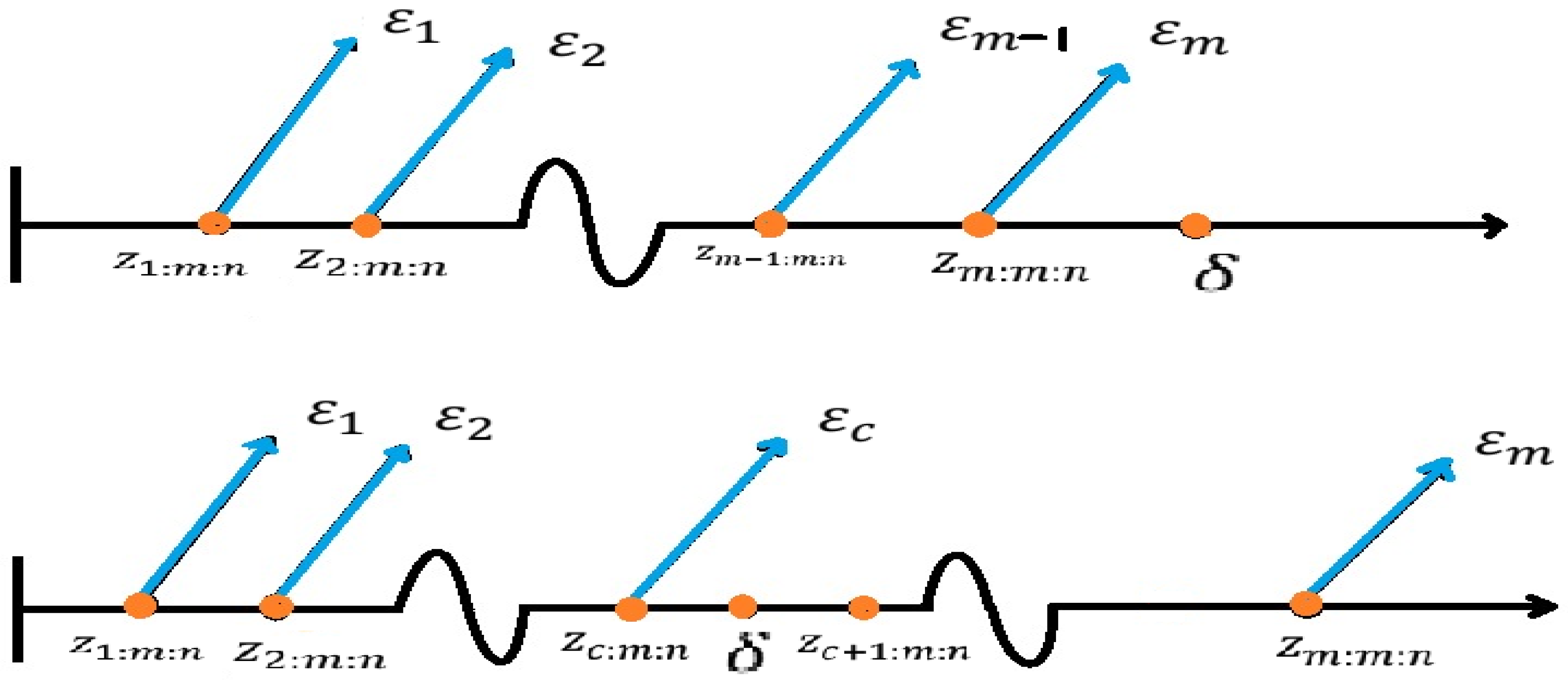
2. Assumptions and Procedure for Testing
3. The Parameter Estimation
4. Confidence Intervals
4.1. Approximate Confidence Intervals
4.2. Bootstrap Confidence Intervals
| Algorithm 1. Bootstrap |
| 1. Step 0, basic setup: |
| 2. Set b = 1 3. Determine the MLE values of , as showing by . 4. Step 1: Sample 5. Get the bootstrap resample from , where is the MLE from Step 0. 6. Step 2: Estimates from the bootstrap: 7. Calculate the bootstrap estimations. 8. 9. Utilize the resample obtained in Step 1. 10. Step three, repeat: 11. Set b←b+1, 12. Steps 1–3 are then repeated until b = G. 13. Step 4: In ascending sequence, begin: 14. Sort the estimates in increasing order so that 15. |
5. Bayesian Estimation
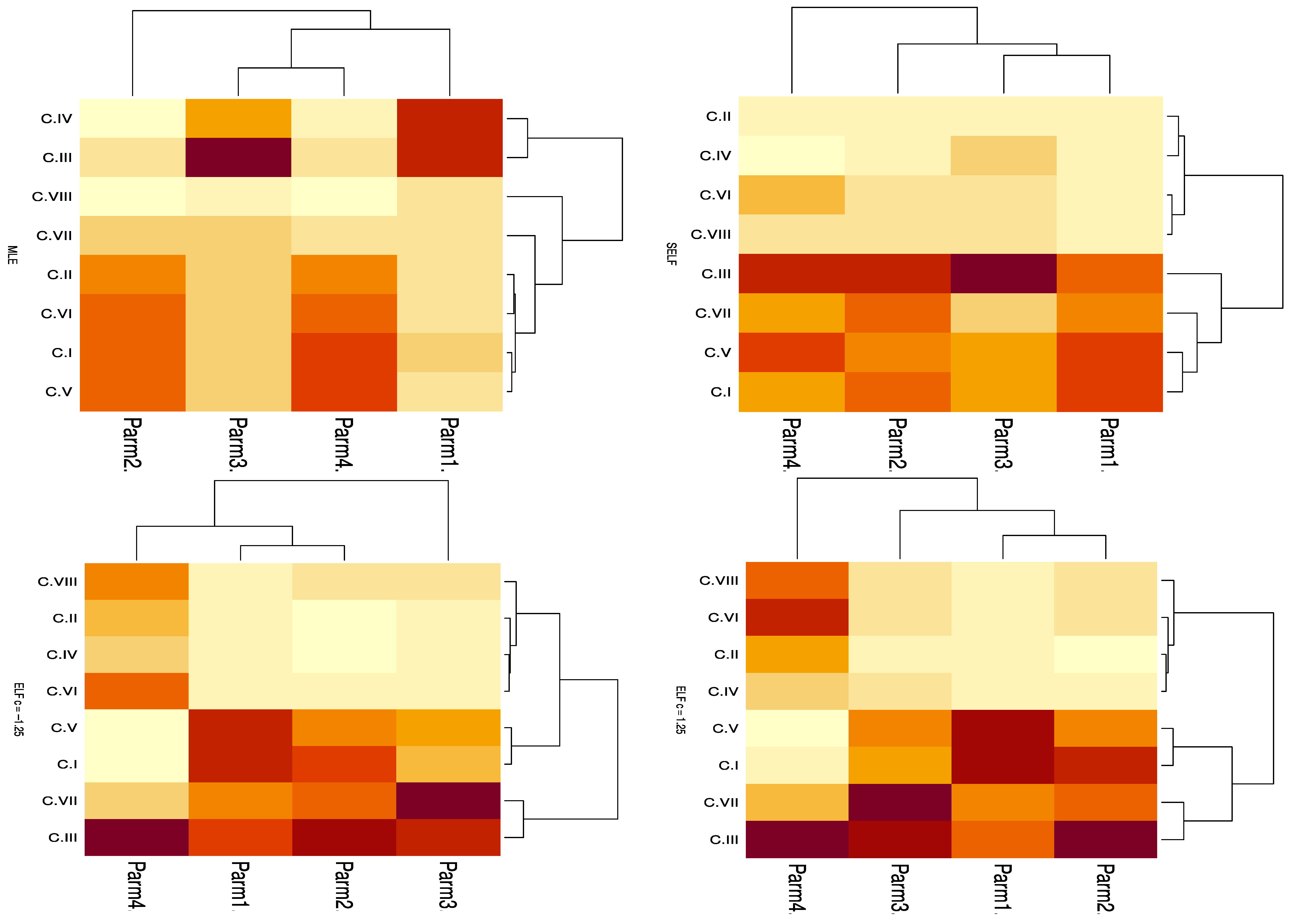
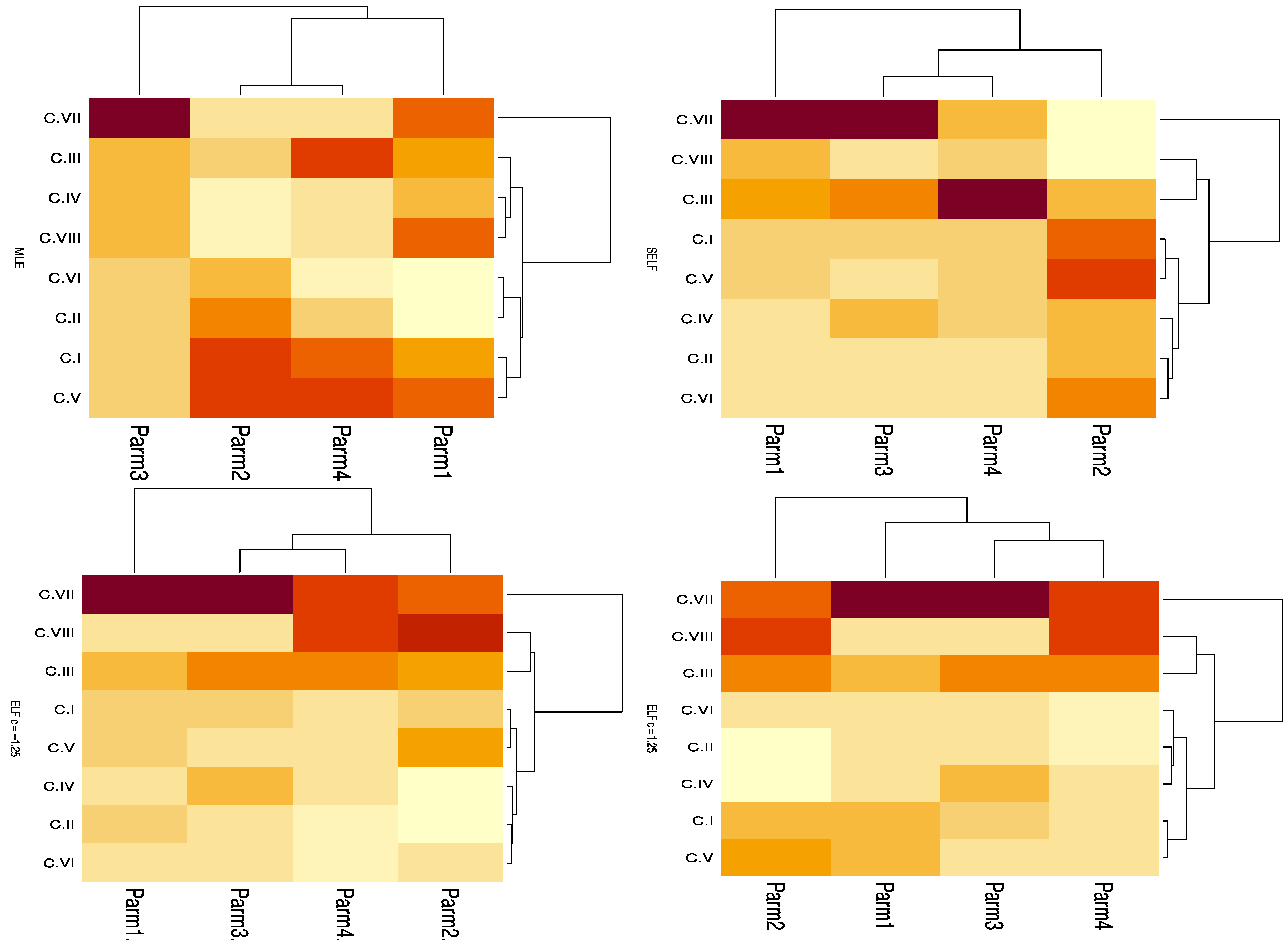
6. Optimization Criterion
7. Simulation
- Give the numbers n, m, and . The total sample size in complete case is n = 100 and 200; the censored sample size is m = 75 and 90 m when n = 100 and m = 150 and 185 when n = 200.
- Give the parameters, , and .
- Make a sample of size n of the randomness from the random variable t in Equation (1), then sort it. It is easy to create a random variable with the APIW distribution. If the uniform random variable U is drawn from the interval [0, 1], then
- To generate the adaptive progressive hybrid censored data for given n, m, and , we use the model in (7). The data can be thought of as:
- To obtain the MLEs of the parameters, the nonlinear system is solved by using the Newton–Raphson method.
- To obtain the Bayes estimation of the parameters, we obtain posterior samples from the MCMC algorithm.
- Repeat Steps 3 through 6 for 1000 iterations.
- Calculate the MLEs and Bayes parameter-related average values of bias, MSE, and LCI.
- Calculate various parameter estimations and their confidence intervals.
- Calculate the various optimization criteria.
- By increasing the censored sample sizes m, the bias, MSE, and LCI of the estimates for the two alternative censored methods decrease for fixed values of n and .
- By increasing the censored sample sizes , the bias, MSE, and LCI of the estimates for the two alternative censored methods decrease for fixed values of n and .
- By increasing the censored sample sizes n, the bias, MSE, and LCI of the estimates for the two alternative censored methods decrease for fixed values of the sample sizes and .
- Bayes estimations of the parameters under the two loss functions outperform the MLE in terms of bias and MSE for the scenarios under consideration.
- The bias and MSE of Bayes estimations of the parameters increase under the considered scenarios when we used negative weight for ELF.
- The HPDs of the unknown parameters outperform the CIs based on the MLEs with respect to ACIs and LCIs. In addition, we observe that the lengths of the bootstrap CIs are the shortest.
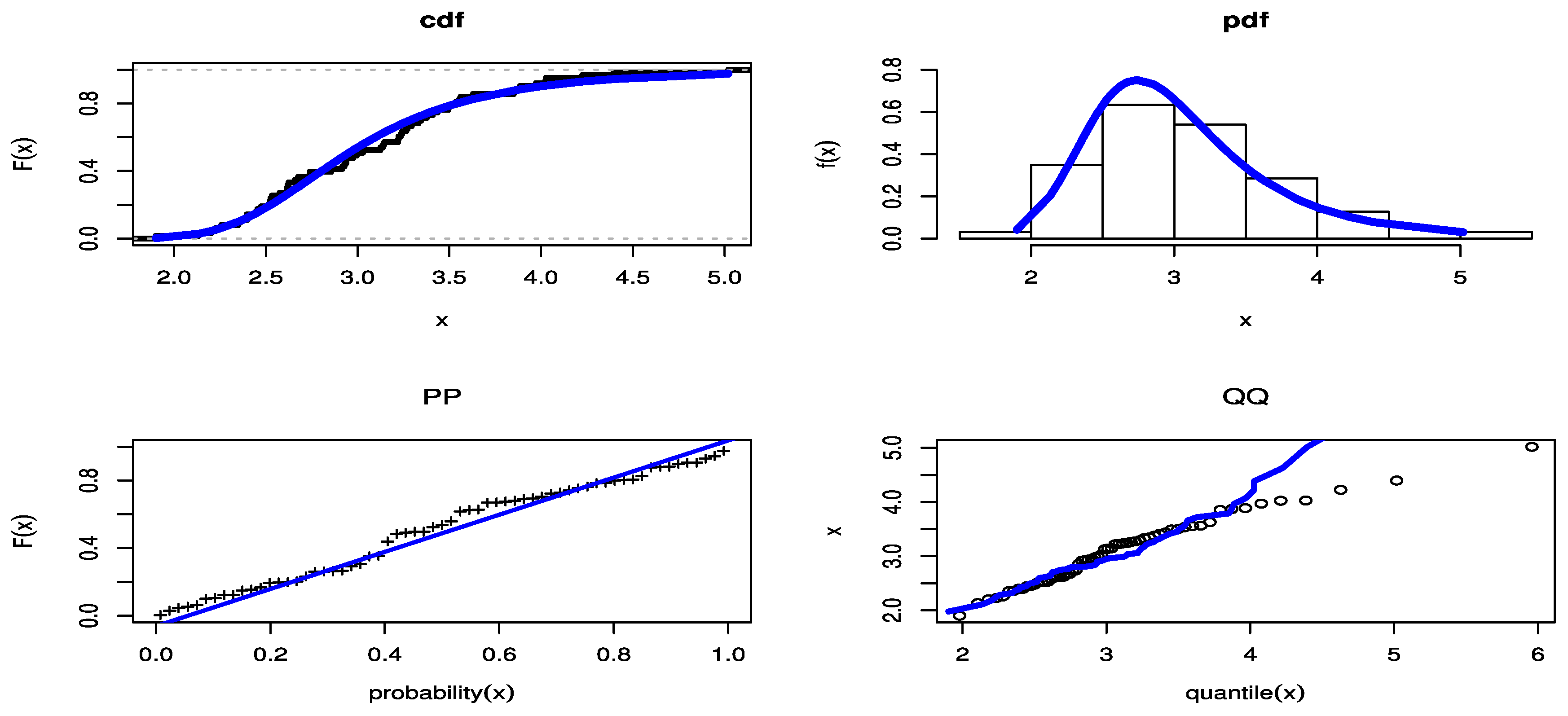
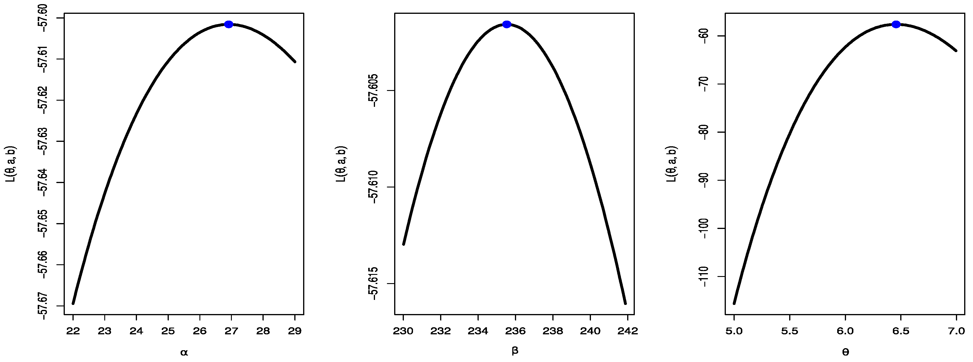
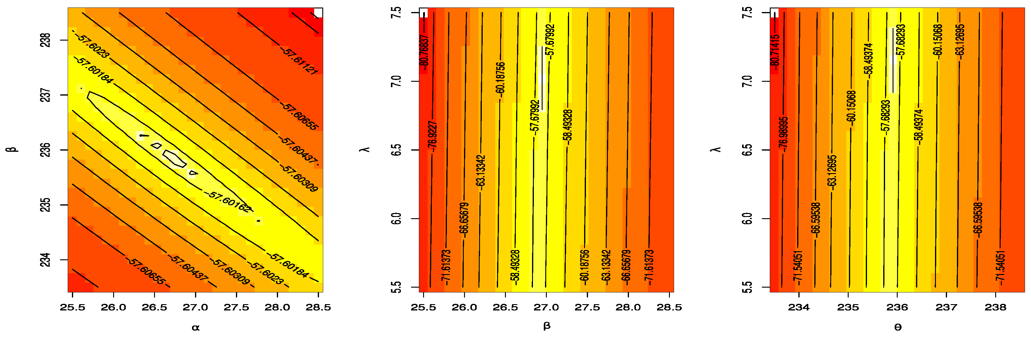
8. A Real-Data Application
- Find the maximum likelihood estimate of the unknown parameter , denoted by , under the hypothesized model and calculate for .
- Generate as for .
- Considering as a progressively Type-II censored data from an APIW distribution with and calculate the maximum likelihood estimates .
- Calculate for .
- Calculate
- Reject the null hypothesis at significance level if the test statistic exceeds the upper tail significance points.
9. Conclusions
Author Contributions
Funding
Institutional Review Board Statement
Informed Consent Statement
Data Availability Statement
Acknowledgments
Conflicts of Interest
Appendix A. Fisher Information Matrix
References
- Rahman, A.; Sindhu, T.N.; Lone, S.A.; Kamal, M. Statistical inference for Burr Type X distribution using geometric process in accelerated life testing design for time censored data. Pak. J. Stat. Oper. Res. 2020, 16, 577–586. [Google Scholar] [CrossRef]
- Zhang, X.; Yang, J.; Kong, X. Planning constant-stress accelerated life tests with multiple stresses based on D-optimal design. Qual. Reliab. Eng. Int. 2021, 37, 60–77. [Google Scholar] [CrossRef]
- Dusmez, S.; Akin, B. Remaining useful lifetime estimation for degraded power MOSFETs under cyclic thermal stress. In Proceedings of the 2015 IEEE Energy Conversion Congress and Exposition (ECCE), Montreal, QC, Canada, 20–24 September 2015; pp. 3846–3851. [Google Scholar] [CrossRef]
- Stojadinovic, N.; Dankovic, D.; Manic, I.; Davidovic, V.; Djoric-Veljkovic, S.; Golubovic, S. Impact of Negative Bias Temperature Instabilities on Lifetime in p-channel Power VDMOSFETs. In Proceedings of the 2007 8th International Conference on Telecommunications in Modern Satellite, Cable and Broadcasting Services, Nis, Serbia and Montenegro, 26–28 September 2007; pp. 275–282. [Google Scholar] [CrossRef]
- Alotaibi, R.; Mutairi, A.; Almetwally, E.M.; Park, C.; Rezk, H. Optimal Design for a Bivariate Step-Stress Accelerated Life Test with Alpha Power Exponential Distribution Based on Type-I Progressive Censored Samples. Symmetry 2022, 14, 830. [Google Scholar] [CrossRef]
- Hassan, A.S.; Nassr, S.G.; Pramanik, S.; Maiti, S.S. Estimation in constant stress partially accelerated life tests for Weibull distribution based on censored competing risks data. Ann. Data Sci. 2020, 7, 45–62. [Google Scholar] [CrossRef]
- Rabie, A. E-Bayesian estimation for a constant-stress partially accelerated life test based on Burr-X Type-I hybrid censored data. J. Stat. Manag. Syst. 2021, 24, 1649–1667. [Google Scholar] [CrossRef]
- Goel, P.K. Some Estimation Problems in the Study of Tampered Random Variables. Ph.D. Thesis, Department of Statistics, Carnegie Mellon University, Pittsburgh, Pennsylvania, 1971. [Google Scholar]
- DeGroot, M.H.; Goel, P.K. Bayesian estimation and optimal designs in partially accelerated life testing. Nav. Res. Logist. 1979, 26, 223–235. [Google Scholar] [CrossRef]
- Rahman, A.; Lone, S.A.; Islam, A. Analysis of exponentiated exponential model under step stress partially accelerated life testing plan using progressive type-II censored data. Investig. Oper. 2019, 39, 551–559. [Google Scholar]
- Epstein, B. Truncated life tests in the exponential case. Ann. Math. Stat. 1954, 25, 555–564. [Google Scholar] [CrossRef]
- Balakrishnan, N.; Kundu, D. Hybrid censoring: Models, inferential results and applications. Comput. Stat. Data Anal. 2013, 57, 166–209. [Google Scholar] [CrossRef]
- Balakrishnan, N. Progressive censoring methodology: An appraisal. Test 2007, 16, 211–296. [Google Scholar] [CrossRef]
- Balakrishnan, N.; Cramer, E. The Art of Progressive Censoring: Applications to Reliability and Quality, Statistics for Industry and Technology; Springer: New York, NY, USA, 2014. [Google Scholar]
- Kundu, D.; Joarder, A. Analysis of Type-II progressively hybrid censored data. Comput. Stat. Data Anal. 2006, 50, 2509–2528. [Google Scholar] [CrossRef]
- Ng, H.K.T.; Kundu, D.; Chan, P.S. Statistical analysis of exponential lifetimes under an adaptive Type-II progressive censoring scheme. Nav. Res. Logist. (NRL) 2009, 56, 687–698. [Google Scholar] [CrossRef] [Green Version]
- Lin, C.T.; Ng, H.K.T.; Chan, P.S. Statistical inference of Type-II progressively hybrid censored data with Weibull lifetimes. Commun. Stat. Meth. 2009, 38, 1710–1729. [Google Scholar] [CrossRef]
- Ismail, A.A. Inference for a step-stress partially accelerated life test model with an adaptive Type-II progressively hybrid censored data from Weibull distribution. J. Comput. Appl. Math. 2014, 260, 533–542. [Google Scholar] [CrossRef]
- Almetwally, E.M.; Almongy, H.M.; Rastogi, M.K.; Ibrahim, M. Maximum product spacing estimation of Weibull distribution under adaptive type-II progressive censoring schemes. Ann. Data Sci. 2020, 7, 257–279. [Google Scholar] [CrossRef]
- Hemmati, F.; Khorram, E. Statistical analysis of the lognormal distribution under type-II progressive hybrid censoring schemes. Commun. Stat. Simulat. Comput. 2013, 42, 52–75. [Google Scholar] [CrossRef]
- Sobhi, M.M.A.; Soliman, A.A. Estimation for the exponentiated Weibull model with adaptive Type-II progressive censored schemes. Appl. Math. Model. 2016, 40, 1180–1192. [Google Scholar] [CrossRef]
- Zhang, C.; Shi, Y. Estimation of the extended Weibull parameters and acceleration factors in the step-stress accelerated life tests under an adaptive progressively hybrid censoring data. J. Stat. Comput. Simulat. 2016, 86, 3303–3314. [Google Scholar] [CrossRef]
- Nassr, S.G.; Almetwally, E.M.; El Azm, W.S.A. Statistical inference for the extended Weibull distribution based on adaptive type-II progressive hybrid censored competing risks data. Thail. Stat. 2021, 19, 547–564. [Google Scholar]
- Nassar, M.; Nassr, S.G.; Dey, S. Analysis of burr Type-XII distribution under step stress partially accelerated life tests with Type-I and adaptive Type-II progressively hybrid censoring schemes. Ann. Data Sci. 2017, 4, 227–248. [Google Scholar] [CrossRef]
- Abo-Kasem, O.E.; Almetwally, E.M.; Abu El Azm, W.S. Inferential Survival Analysis for Inverted NH Distribution Under Adaptive Progressive Hybrid Censoring with Application of Transformer Insulation. Ann. Data Sci. 2022, 1–48. [Google Scholar] [CrossRef]
- Alam, I.; Ahmed, A. Parametric and Interval Estimation Under Step-Stress Partially Accelerated Life Tests Using Adaptive Type-II Progressive Hybrid Censoring. Ann. Data Sci. 2020, 1–13. [Google Scholar] [CrossRef]
- Almongy, H.M.; Almetwally, E.M.; Alharbi, R.; Alnagar, D.; Hafez, E.H.; Mohie El-Din, M.M. The Weibull generalized exponential distribution with censored sample: Estimation and application on real data. Complexity 2021, 2021, 6653534. [Google Scholar] [CrossRef]
- Selim, M.A. Estimation and prediction for Nadarajah-Haghighi distribution based on record values. Pak. J. Stat. 2018, 34, 77–90. [Google Scholar] [CrossRef]
- Haj Ahmad, H.; Salah, M.M.; Eliwa, M.S.; Ali Alhussain, Z.; Almetwally, E.M.; Ahmed, E.A. Bayesian and non-Bayesian inference under adaptive type-II progressive censored sample with exponentiated power Lindley distribution. J. Appl. Stat. 2022, 49, 2981–3001. [Google Scholar] [CrossRef] [PubMed]
- Basheer, A.M. Marshall-Olkin alpha power inverse exponential distribution: Properties and applications. Ann. Data Sci. 2019, 9, 301–313. [Google Scholar] [CrossRef]
- Neyman, J. Outline of a theory of statistical estimation based on the classical theory of probability. Philos. Trans. R. Soc. Lond.-Ser. A Math. Phys. Sci. 1937, 236, 333–380. [Google Scholar]
- Efron, B. Bootstrap Methods: Another Look at the Jackknife. Ann. Stat. 1979, 7, 1–26. [Google Scholar] [CrossRef]
- Gelman, A.; Carlin, J.B.; Stern, H.S.; Rubin, D.B. Bayesian Data Analysis, 2nd ed.; Chapman and Hall/CRC: Boca Raton, FL, USA, 2004. [Google Scholar] [CrossRef]
- Dey, S. Bayesian estimation of the shape parameter of the generalized exponential distribution under different loss functions. Pak. J. Stat. Oper. Res. 2010, 6, 163–174. [Google Scholar] [CrossRef] [Green Version]
- Burkschat, M.; Cramer, E.; Kamps, U. On optimal schemes in progressive censoring. Stat. Probab. Lett. 2006, 76, 1032–1036. [Google Scholar] [CrossRef]
- Burkschat, M.; Cramer, E.; Kamps, U. Optimality criteria and optimal schemes in progressive censoring. Commun. Stat.—Theory Methods 2007, 36, 1419–1431. [Google Scholar] [CrossRef]
- Burkschat, M. On optimality of extremal schemes in progressive type II censoring. J. Stat. Plan. Inference 2008, 138, 1647–1659. [Google Scholar] [CrossRef]
- Pradhan, B.; Kundu, D. On progressively censored generalized exponential distribution. TEST 2009, 18, 497–515. [Google Scholar] [CrossRef]
- Elshahhat, A.; Rastogi, M.K. Estimation of parameters of life for an inverted Nadarajah–Haghighi distribution from type-II progressively censored samples. J. Indian Soc. Probab. Stat. 2021, 22, 113–154. [Google Scholar] [CrossRef]
- Long, C.; Chen, W.; Yang, R. Ratio estimation of the population mean using auxiliary information under the optimal sampling design. Probab. Eng. Inf. Sci. 2022, 36, 449–460. [Google Scholar] [CrossRef]
- Badar, M.G.; Priest, A.M. Statistical aspects of fibre and bundle strength in hybrid composites. In Progress in Science and Engineering Composites; Hayashi, T., Kawata, K., Umekawa, S., Eds.; ICCM-IV: Tokyo, Japan, 1982; pp. 1129–1136. [Google Scholar]
- Chen, G.; Balakrishnan, N. A general-purpose approximate goodness-of-fit test. J. Qual. Technol. 1995, 27, 154–161. [Google Scholar] [CrossRef]
- Pakyari, R.; Balakrishnan, N. A general-purpose approximate goodness-of-fit test for progressively type-II censored data. IEEE Trans. Reliab. 2012, 61, 238–244. [Google Scholar] [CrossRef]
- El-Din, M.M.; Abu-Youssef, S.E.; Ali, N.S.; Abd El-Raheem, A.M. Estimation in constant-stress accelerated life tests for extension of the exponential distribution under progressive censoring. Metron 2016, 74, 253–273. [Google Scholar] [CrossRef]
- Abd El-Raheem, A.M.; Almetwally, E.M.; Mohamed, M.S.; Hafez, E.H. Accelerated life tests for modified Kies exponential lifetime distribution: Binomial removal, transformers turn insulation application and numerical results. AIMS Math. 2021, 6, 5222–5255. [Google Scholar] [CrossRef]
- Dimitrova, D.S.; Kaishev, V.K.; Tan, S. Computing the Kolmogorov-Smirnov Distribution When the Underlying CDF is Purely Discrete, Mixed, or Continuous. J. Sta. Softw. 2020, 95, 1–42. [Google Scholar] [CrossRef]


| Criterion | Method |
| Maximize trace | |
| Minimize trace | |
| Minimize det |
| MLE | SELF | ELF c = −1.25 | ELF c = 1.25 | ||||||||||||||
|---|---|---|---|---|---|---|---|---|---|---|---|---|---|---|---|---|---|
| n | m | Bias | MSE | LACI | LBPCI | LBTCI | Bias | MSE | LCCI | Bias | MSE | LCCI | Bias | MSE | LCCI | ||
| 100 | 2, 10 | 75 | 0.3263 | 0.3997 | 2.1248 | 0.0965 | 0.0947 | −0.2602 | 0.3062 | 1.8368 | −0.2458 | 0.2894 | 1.7968 | −0.4100 | 0.5367 | 2.2491 | |
| −1.3825 | 1.9408 | 0.6726 | 0.0302 | 0.0301 | −0.5628 | 0.3439 | 0.6222 | −0.5578 | 0.3379 | 0.6157 | −0.6050 | 0.3980 | 0.6726 | ||||
| −0.3294 | 0.1665 | 0.9447 | 0.0406 | 0.0406 | 0.2863 | 0.1435 | 0.7539 | 0.6361 | 0.4416 | 0.7597 | 0.5878 | 0.3778 | 0.6959 | ||||
| 0.8792 | 0.8010 | 0.6577 | 0.0301 | 0.0300 | 0.0546 | 0.0395 | 0.3513 | 0.0563 | 0.0097 | 0.3143 | 0.0389 | 0.0079 | 0.3100 | ||||
| 90 | 0.1289 | 0.3267 | 2.1851 | 0.1033 | 0.1031 | −0.0321 | 0.0331 | 0.7063 | −0.0309 | 0.0329 | 0.7056 | −0.0423 | 0.0351 | 0.7149 | |||
| −1.3616 | 1.8885 | 0.7287 | 0.0325 | 0.0327 | −0.2817 | 0.1017 | 0.5869 | −0.2789 | 0.0997 | 0.5807 | −0.3071 | 0.1212 | 0.6382 | ||||
| −0.2883 | 0.1568 | 1.0653 | 0.0484 | 0.0484 | 0.1990 | 0.0575 | 0.5284 | 0.2005 | 0.0583 | 0.5303 | 0.1850 | 0.0506 | 0.4982 | ||||
| θ | 0.8403 | 0.7273 | 0.5710 | 0.0257 | 0.0253 | 0.0464 | 0.0241 | 0.3401 | 0.1281 | 0.0246 | 0.3411 | 0.1123 | 0.0198 | 0.3214 | |||
| 3.5, 18 | 75 | 1.2072 | 2.6719 | 4.3243 | 0.1911 | 0.1921 | −0.1065 | 0.2610 | 1.8586 | −0.0961 | 0.2537 | 1.8425 | −0.2112 | 0.3636 | 2.1097 | ||
| −1.1084 | 1.2923 | 0.9910 | 0.0427 | 0.0432 | −0.6102 | 0.4100 | 0.7449 | −0.6050 | 0.4028 | 0.7387 | −0.6526 | 0.4709 | 0.7836 | ||||
| λ | 0.4902 | 0.4963 | 1.9853 | 0.0901 | 0.0900 | 0.2893 | 0.2940 | 0.6019 | 0.9399 | 0.9551 | 1.0307 | 0.8542 | 0.7929 | 0.9038 | |||
| 0.6934 | 0.5379 | 0.9372 | 0.0414 | 0.0410 | 0.1369 | 0.0546 | 0.4633 | 0.1387 | 0.0560 | 0.4645 | 0.1201 | 0.0390 | 0.4486 | ||||
| 90 | 1.3165 | 2.5775 | 3.6059 | 0.1659 | 0.1640 | −0.0176 | 0.0289 | 0.6324 | −0.0166 | 0.0288 | 0.6321 | −0.0262 | 0.0298 | 0.6365 | |||
| β | −0.7230 | 0.9408 | 0.6724 | 0.0317 | 0.0317 | −0.2981 | 0.1098 | 0.5521 | −0.2953 | 0.1077 | 0.5458 | −0.3236 | 0.1297 | 0.6095 | |||
| 0.3408 | 0.2248 | 1.2936 | 0.0615 | 0.0615 | 0.2828 | 0.0994 | 0.5239 | 0.2850 | 0.1009 | 0.5256 | 0.2630 | 0.0863 | 0.4918 | ||||
| 0.5154 | 0.5080 | 0.4873 | 0.0216 | 0.0217 | 0.1171 | 0.0185 | 0.2572 | 0.1185 | 0.0188 | 0.2583 | 0.1050 | 0.0154 | 0.2438 | ||||
| 200 | 2, 10 | 150 | 0.4348 | 0.3536 | 1.5917 | 0.0687 | 0.0686 | −0.3758 | 0.3113 | 1.5792 | −0.3615 | 0.2930 | 1.5336 | −0.5182 | 0.5351 | 1.9342 | |
| −1.4213 | 2.0289 | 0.3648 | 0.0164 | 0.0164 | −0.5234 | 0.2866 | 0.4452 | −0.5207 | 0.2836 | 0.4421 | −0.5462 | 0.3127 | 0.4733 | ||||
| −0.3996 | 0.1784 | 0.5367 | 0.0252 | 0.0251 | 0.3067 | 0.1470 | 0.4559 | 0.6752 | 0.4750 | 0.5652 | 0.6380 | 0.4234 | 0.5026 | ||||
| 0.8859 | 0.7991 | 0.4679 | 0.0216 | 0.0216 | 0.1493 | 0.0536 | 0.2133 | 0.0502 | 0.0055 | 0.2140 | 0.0411 | 0.0046 | 0.2089 | ||||
| 185 | 0.3155 | 0.2366 | 1.4526 | 0.0660 | 0.0657 | −0.0758 | 0.0305 | 0.6101 | −0.0749 | 0.0303 | 0.6091 | −0.0847 | 0.0331 | 0.6135 | |||
| −1.4129 | 2.0049 | 0.3619 | 0.0153 | 0.0150 | −0.3626 | 0.1448 | 0.4347 | −0.3595 | 0.1423 | 0.4300 | −0.3899 | 0.1677 | 0.4811 | ||||
| −0.3822 | 0.1643 | 0.5300 | 0.0236 | 0.0241 | 0.2720 | 0.0855 | 0.4317 | 0.2737 | 0.0866 | 0.4337 | 0.2565 | 0.0760 | 0.4061 | ||||
| 0.8609 | 0.7536 | 0.4379 | 0.0193 | 0.0194 | 0.1081 | 0.0367 | 0.2046 | 0.1822 | 0.0372 | 0.2442 | 0.1678 | 0.0318 | 0.2363 | ||||
| 3.5, 18 | 150 | 0.4026 | 0.2824 | 1.4873 | 0.0552 | 0.0567 | −0.1721 | 0.2094 | 1.5946 | −0.1630 | 0.2006 | 1.5636 | −0.2593 | 0.3096 | 1.8659 | ||
| −0.9198 | 1.4616 | 0.3652 | 0.0129 | 0.0128 | −0.5550 | 0.3255 | 0.5263 | −0.5521 | 0.3219 | 0.5242 | −0.5792 | 0.3553 | 0.5561 | ||||
| 0.2994 | 0.1698 | 0.5294 | 0.0258 | 0.0255 | 0.1025 | 0.1085 | 0.4657 | 1.0326 | 1.1012 | 0.6591 | 0.9497 | 0.9289 | 0.5761 | ||||
| 0.7250 | 0.5558 | 0.6811 | 0.0314 | 0.0309 | 0.1129 | 0.0419 | 0.2710 | 0.1138 | 0.0197 | 0.2710 | 0.1047 | 0.0168 | 0.2699 | ||||
| 185 | 0.4004 | 0.2704 | 1.0908 | 0.0425 | 0.0416 | −0.0208 | 0.0234 | 0.5713 | −0.0200 | 0.0233 | 0.5702 | −0.0283 | 0.0244 | 0.5746 | |||
| −0.2134 | 0.8482 | 0.3493 | 0.0109 | 0.0119 | −0.3858 | 0.1599 | 0.3899 | −0.3823 | 0.1570 | 0.3850 | −0.4166 | 0.1867 | 0.4370 | ||||
| 0.2444 | 0.0915 | 0.5070 | 0.0219 | 0.0214 | 0.2369 | 0.0877 | 0.4251 | 0.3718 | 0.1509 | 0.4277 | 0.3447 | 0.1295 | 0.3881 | ||||
| 0.6121 | 0.4589 | 0.3919 | 0.0174 | 0.0174 | 0.1670 | 0.0305 | 0.1924 | 0.1681 | 0.0309 | 0.1941 | 0.1565 | 0.0268 | 0.1823 | ||||
| MLE | SELF | ELF c = −1.25 | ELF c = 1.25 | ||||||||||||||
|---|---|---|---|---|---|---|---|---|---|---|---|---|---|---|---|---|---|
| n | m | Bias | MSE | LACI | LBPCI | LBTCI | Bias | MSE | LCCI | Bias | MSE | LCCI | Bias | MSE | LCCI | ||
| 100 | 2, 10 | 75 | 0.4624 | 0.5714 | 2.3474 | 0.1201 | 0.1205 | −0.2218 | 0.2633 | 1.8289 | −0.2105 | 0.2495 | 1.7748 | −0.3394 | 0.4512 | 2.2924 | |
| −1.3916 | 1.9624 | 0.6328 | 0.0319 | 0.0321 | −0.5221 | 0.2971 | 0.6066 | −0.5175 | 0.2918 | 0.5994 | −0.5610 | 0.3430 | 0.6561 | ||||
| −0.3496 | 0.1814 | 0.9551 | 0.0496 | 0.0499 | 0.3042 | 0.1802 | 0.7407 | 0.4214 | 0.2150 | 0.7430 | 0.3813 | 0.1781 | 0.7106 | ||||
| 1.0136 | 1.0650 | 0.7624 | 0.0425 | 0.0421 | 0.5739 | 0.3628 | 0.7099 | 0.5790 | 0.3695 | 0.7194 | 0.5214 | 0.2973 | 0.6187 | ||||
| 90 | 0.5295 | 0.5660 | 2.4170 | 0.0765 | 0.0770 | −0.2670 | 0.2579 | 1.7531 | −0.2544 | 0.2632 | 1.6937 | −0.4003 | 0.5122 | 2.3486 | |||
| −1.4030 | 1.9596 | 0.6540 | 0.0210 | 0.0206 | −0.5261 | 0.2965 | 0.5475 | −0.5217 | 0.2915 | 0.5396 | −0.5636 | 0.3405 | 0.5825 | ||||
| −0.3740 | 0.1798 | 1.3282 | 0.0431 | 0.0425 | 0.4374 | 0.1800 | 0.7370 | 0.4412 | 0.2313 | 0.7418 | 0.4023 | 0.1940 | 0.6995 | ||||
| 0.9861 | 1.0122 | 0.7831 | 0.0251 | 0.0249 | 0.5751 | 0.3640 | 0.6653 | 0.5798 | 0.3701 | 0.6715 | 0.5259 | 0.3017 | 0.6024 | ||||
| 3.5, 18 | 75 | 0.4601 | 0.5524 | 2.2904 | 0.1124 | 0.1125 | −0.1171 | 0.2100 | 1.6852 | −0.1090 | 0.2033 | 1.6784 | −0.1962 | 0.2943 | 1.8787 | ||
| −1.1979 | 1.4732 | 0.7660 | 0.0243 | 0.0246 | −0.5480 | 0.2832 | 0.5410 | −0.5432 | 0.3140 | 0.5365 | −0.5884 | 0.3679 | 0.5782 | ||||
| 0.2992 | 0.1722 | 0.9408 | 0.0444 | 0.0438 | 0.6883 | 0.1526 | 0.9032 | 0.6950 | 0.5369 | 0.9078 | 0.6229 | 0.4307 | 0.8363 | ||||
| 0.8304 | 0.7148 | 0.6230 | 0.0188 | 0.0188 | 0.4609 | 0.2310 | 0.5173 | 0.4644 | 0.2346 | 0.5208 | 0.4256 | 0.1959 | 0.4685 | ||||
| 90 | 0.5074 | 0.5339 | 2.2637 | 0.0712 | 0.0716 | −0.0227 | 0.0252 | 0.5770 | −0.0219 | 0.0251 | 0.5750 | −0.0300 | 0.0263 | 0.5855 | |||
| −1.1968 | 1.4705 | 0.7666 | 0.0240 | 0.0241 | −0.2323 | 0.0708 | 0.5093 | −0.2303 | 0.0697 | 0.5044 | −0.2500 | 0.0822 | 0.5517 | ||||
| 0.2893 | 0.1719 | 0.9128 | 0.0292 | 0.0298 | 0.2058 | 0.0585 | 0.4962 | 0.2073 | 0.0593 | 0.4986 | 0.1917 | 0.0513 | 0.4786 | ||||
| 0.8319 | 0.7175 | 0.6251 | 0.0204 | 0.0205 | 0.2410 | 0.0649 | 0.3098 | 0.2432 | 0.0661 | 0.3141 | 0.2204 | 0.0542 | 0.2832 | ||||
| 200 | 2, 10 | 150 | 0.4968 | 0.4611 | 1.8157 | 0.0594 | 0.0594 | −0.4156 | 0.3868 | 1.7927 | −0.3966 | 0.3570 | 1.7173 | −0.6259 | 0.8221 | 2.3011 | |
| −1.4238 | 2.0385 | 0.4153 | 0.0131 | 0.0131 | −0.5478 | 0.3116 | 0.4096 | −0.5445 | 0.3078 | 0.4078 | −0.5748 | 0.3434 | 0.4355 | ||||
| −0.4137 | 0.1950 | 0.6052 | 0.0186 | 0.0184 | 0.4819 | 0.1826 | 0.5607 | 0.4852 | 0.2608 | 0.6138 | 0.4507 | 0.2244 | 0.5572 | ||||
| 0.9426 | 0.9101 | 0.5755 | 0.0177 | 0.0173 | 0.5626 | 0.3389 | 0.5679 | 0.5658 | 0.3428 | 0.5713 | 0.5291 | 0.2985 | 0.5178 | ||||
| 185 | 0.5008 | 0.4615 | 1.8002 | 0.0559 | 0.0563 | −0.0585 | 0.0268 | 0.5996 | −0.0576 | 0.0265 | 0.5964 | −0.0668 | 0.0293 | 0.6242 | |||
| −1.4305 | 2.0554 | 0.3718 | 0.0120 | 0.0118 | −0.3356 | 0.1240 | 0.4175 | −0.3328 | 0.1220 | 0.4126 | −0.3604 | 0.1433 | 0.4485 | ||||
| −0.4246 | 0.1920 | 0.5577 | 0.0183 | 0.0180 | 0.2406 | 0.0689 | 0.4180 | 0.2421 | 0.0698 | 0.4216 | 0.2260 | 0.0609 | 0.3888 | ||||
| 0.9422 | 0.9061 | 0.5310 | 0.0167 | 0.0167 | 0.3808 | 0.1519 | 0.3178 | 0.3844 | 0.1548 | 0.3210 | 0.3454 | 0.1245 | 0.2811 | ||||
| 3.5, 18 | 150 | 0.4717 | 0.3649 | 1.7284 | 0.0574 | 0.0570 | −0.2171 | 0.2180 | 1.5888 | −0.2071 | 0.2071 | 1.5436 | −0.3190 | 0.3637 | 2.0831 | ||
| −1.2425 | 1.5586 | 0.4772 | 0.0152 | 0.0148 | −0.5556 | 0.3018 | 0.3705 | −0.5524 | 0.3143 | 0.3680 | −0.5818 | 0.3487 | 0.3847 | ||||
| 0.1907 | 0.0833 | 0.8496 | 0.0252 | 0.0254 | 0.8361 | 0.0733 | 0.7085 | 0.8428 | 0.7451 | 0.7166 | 0.7687 | 0.6179 | 0.6418 | ||||
| 0.7916 | 0.6403 | 0.4600 | 0.0147 | 0.0148 | 0.4665 | 0.2287 | 0.4089 | 0.4688 | 0.2310 | 0.4112 | 0.4432 | 0.2060 | 0.3780 | ||||
| 185 | 1.5699 | 0.3267 | 3.5125 | 0.1158 | 0.1166 | −0.0406 | 0.0260 | 0.6052 | −0.0398 | 0.0259 | 0.6024 | −0.0483 | 0.0275 | 0.6174 | |||
| −1.2296 | 1.5242 | 0.4327 | 0.0146 | 0.0144 | −0.3682 | 0.1148 | 0.4297 | −0.3648 | 0.1450 | 0.4256 | −0.3978 | 0.1727 | 0.4703 | ||||
| 0.2119 | 0.0832 | 0.7672 | 0.0246 | 0.0253 | 0.3420 | 0.0513 | 0.4309 | 0.3447 | 0.1319 | 0.4339 | 0.3172 | 0.1117 | 0.4069 | ||||
| 0.7923 | 0.6399 | 0.4322 | 0.0138 | 0.0138 | 0.3183 | 0.1058 | 0.2583 | 0.3207 | 0.1074 | 0.2611 | 0.2952 | 0.0908 | 0.2329 | ||||
| MLE | SELF | ELF c = −1.25 | ELF c = 1.25 | ||||||||||||||
|---|---|---|---|---|---|---|---|---|---|---|---|---|---|---|---|---|---|
| n | m | Bias | MSE | LACI | LBPCI | LBTCI | Bias | MSE | LCCI | Bias | MSE | LCCI | Bias | MSE | LCCI | ||
| 100 | 0.6, 1.3 | 75 | −0.5240 | 0.2747 | 0.1405 | 0.0022 | 0.0022 | −0.1110 | 0.0206 | 0.3572 | −0.1057 | 0.0196 | 0.3578 | −0.1615 | 0.0343 | 0.3626 | |
| −0.2999 | 0.0922 | 0.2150 | 0.0086 | 0.0083 | −0.2663 | 0.0740 | 0.2063 | −0.2641 | 0.0728 | 0.2066 | −0.2856 | 0.0848 | 0.2194 | ||||
| 0.0052 | 0.0093 | 0.4453 | 0.0177 | 0.0177 | 0.0200 | 0.0083 | 0.3513 | 0.0222 | 0.0084 | 0.3514 | 0.0008 | 0.0081 | 0.3521 | ||||
| 0.2704 | 0.0885 | 0.4687 | 0.0205 | 0.0209 | 0.0732 | 0.0181 | 0.4339 | 0.0750 | 0.0184 | 0.4339 | 0.0574 | 0.0156 | 0.4351 | ||||
| 90 | −0.4477 | 0.2017 | 0.0482 | 0.0061 | 0.0061 | −0.0486 | 0.0051 | 0.2093 | −0.0475 | 0.0050 | 0.2086 | −0.0591 | 0.0064 | 0.2144 | |||
| −0.2570 | 0.0691 | 0.1885 | 0.0098 | 0.0100 | −0.2212 | 0.0516 | 0.2015 | −0.2192 | 0.0507 | 0.1992 | −0.2383 | 0.0599 | 0.2146 | ||||
| 0.0945 | 0.0082 | 0.3785 | 0.0203 | 0.0203 | 0.0211 | 0.0056 | 0.2751 | 0.0220 | 0.0056 | 0.2750 | 0.0129 | 0.0055 | 0.2783 | ||||
| 0.1132 | 0.0271 | 0.4865 | 0.0212 | 0.0202 | 0.0282 | 0.0104 | 0.3800 | 0.0289 | 0.0105 | 0.3799 | 0.0218 | 0.0099 | 0.3766 | ||||
| 0.8, 1.5 | 75 | −0.5342 | 0.2856 | 0.1804 | 0.0019 | 0.0019 | −0.0505 | 0.0780 | 0.5301 | −0.0449 | 0.0815 | 0.5360 | −0.0990 | 0.0461 | 0.5708 | ||
| −0.1805 | 0.0375 | 0.3960 | 0.0082 | 0.0082 | −0.2799 | 0.0528 | 0.2684 | −0.2775 | 0.0820 | 0.2668 | −0.3001 | 0.0953 | 0.2745 | ||||
| 0.3202 | 0.1212 | 0.8482 | 0.0163 | 0.0161 | 0.1205 | 0.0312 | 0.4830 | 0.1232 | 0.0318 | 0.4820 | 0.0957 | 0.0263 | 0.4838 | ||||
| 0.2652 | 0.0891 | 0.5336 | 0.0169 | 0.0173 | 0.2184 | 0.0708 | 0.5753 | 0.2206 | 0.0720 | 0.5783 | 0.1984 | 0.0606 | 0.5573 | ||||
| 90 | −0.5122 | 0.2644 | 0.0611 | 0.0056 | 0.0057 | −0.0334 | 0.0081 | 0.2086 | −0.0323 | 0.0037 | 0.2086 | −0.0431 | 0.0047 | 0.2083 | |||
| −0.0762 | 0.0160 | 0.2736 | 0.0124 | 0.0127 | −0.2306 | 0.0506 | 0.1998 | −0.2285 | 0.0548 | 0.1982 | −0.2477 | 0.0644 | 0.2139 | ||||
| 0.2548 | 0.1135 | 0.5362 | 0.0258 | 0.0258 | 0.1086 | 0.0193 | 0.3247 | 0.1096 | 0.0195 | 0.3253 | 0.0994 | 0.0171 | 0.3165 | ||||
| 0.0780 | 0.0246 | 0.5238 | 0.0167 | 0.0165 | 0.0940 | 0.0189 | 0.3921 | 0.0949 | 0.0191 | 0.3931 | 0.0858 | 0.0169 | 0.3768 | ||||
| 200 | 0.6, 1.3 | 150 | −0.5503 | 0.3029 | 0.1706 | 0.0008 | 0.0008 | −0.1207 | 0.0200 | 0.2611 | −0.1166 | 0.0189 | 0.2599 | −0.1571 | 0.0303 | 0.2621 | |
| −0.2948 | 0.0882 | 0.1971 | 0.0044 | 0.0044 | −0.2850 | 0.0833 | 0.1726 | −0.2835 | 0.0824 | 0.1715 | −0.2982 | 0.0911 | 0.1726 | ||||
| 0.0074 | 0.0524 | 0.4162 | 0.0089 | 0.0090 | 0.0116 | 0.0057 | 0.2784 | 0.0131 | 0.0057 | 0.2773 | −0.0023 | 0.0057 | 0.2796 | ||||
| 0.3037 | 0.1005 | 0.3554 | 0.0109 | 0.0109 | 0.0952 | 0.0189 | 0.3662 | 0.0964 | 0.0192 | 0.3668 | 0.0848 | 0.0166 | 0.3599 | ||||
| 185 | −0.4551 | 0.2090 | 0.0259 | 0.0055 | 0.0055 | −0.0324 | 0.0051 | 0.0733 | −0.0320 | 0.0014 | 0.0732 | −0.0362 | 0.0017 | 0.0757 | |||
| −0.1976 | 0.0416 | 0.1409 | 0.0063 | 0.0062 | −0.2553 | 0.0663 | 0.1278 | −0.2536 | 0.0654 | 0.1269 | −0.2687 | 0.0734 | 0.1345 | ||||
| 0.2050 | 0.0053 | 0.2817 | 0.0136 | 0.0137 | −0.0202 | 0.0031 | 0.1965 | −0.0193 | 0.0031 | 0.1962 | −0.0277 | 0.0036 | 0.2046 | ||||
| 0.0212 | 0.0074 | 0.3277 | 0.0110 | 0.0110 | 0.0694 | 0.0068 | 0.2919 | 0.0701 | 0.0108 | 0.2922 | 0.0638 | 0.0097 | 0.2890 | ||||
| 0.8, 1.5 | 150 | −0.5588 | 0.3131 | 0.1154 | 0.0054 | 0.0054 | −0.0395 | 0.2423 | 0.8773 | −0.0266 | 0.4469 | 0.8702 | −0.1289 | 0.1863 | 0.8322 | ||
| 0.0655 | 0.0179 | 0.4586 | 0.0212 | 0.0213 | −0.0833 | 0.0109 | 0.3543 | −0.2813 | 0.0898 | 0.4482 | −0.3004 | 0.1008 | 0.4510 | ||||
| 0.8364 | 0.7483 | 0.8673 | 0.0399 | 0.0395 | 0.1402 | 0.0585 | 0.8695 | 0.1427 | 0.0593 | 0.8679 | 0.1171 | 0.0513 | 0.8502 | ||||
| −0.0539 | 0.0232 | 0.5586 | 0.0267 | 0.0267 | 0.2571 | 0.0194 | 0.5065 | 0.2587 | 0.0953 | 0.6570 | 0.2422 | 0.0843 | 0.6294 | ||||
| 185 | −0.5559 | 0.3091 | 0.0279 | 0.0010 | 0.0010 | −0.0218 | 0.0594 | 0.0401 | −0.0214 | 0.0006 | 0.0400 | −0.0256 | 0.0008 | 0.0424 | |||
| −0.0517 | 0.0133 | 0.1916 | 0.0058 | 0.0059 | −0.3182 | 0.0102 | 0.1041 | −0.3169 | 0.1011 | 0.1039 | −0.3293 | 0.1092 | 0.1060 | ||||
| 0.3258 | 0.1151 | 0.3711 | 0.0120 | 0.0120 | 0.0068 | 0.0027 | 0.1917 | 0.0082 | 0.0027 | 0.1917 | −0.0056 | 0.0027 | 0.1963 | ||||
| 0.0429 | 0.0193 | 0.3909 | 0.0122 | 0.0122 | 0.0290 | 0.0190 | 0.3326 | 0.2915 | 0.0924 | 0.3330 | 0.2772 | 0.0838 | 0.3223 | ||||
| MLE | SELF | ELF c = −1.25 | ELF c = 1.25 | ||||||||||||||
|---|---|---|---|---|---|---|---|---|---|---|---|---|---|---|---|---|---|
| n | m | Bias | MSE | LACI | LBPCI | LBTCI | Bias | MSE | LCCI | Bias | MSE | LCCI | Bias | MSE | LCCI | ||
| 100 | 0.6, 1.3 | 75 | −0.6947 | 0.4827 | 0.6661 | 0.0015 | 0.0015 | −0.0664 | 0.0453 | 0.6946 | −0.0642 | 0.0425 | 0.6770 | −0.0647 | 0.0439 | 0.6710 | |
| −0.2988 | 0.0909 | 0.1620 | 0.0357 | 0.0364 | −0.3179 | 0.0906 | 0.3675 | −0.3146 | 0.0902 | 0.3623 | −0.2934 | 0.0901 | 0.3400 | ||||
| −0.0135 | 0.0093 | 0.3837 | 0.0865 | 0.0825 | −0.1626 | 0.0090 | 0.4409 | −0.1595 | 0.0383 | 0.4353 | −0.1589 | 0.0085 | 0.4282 | ||||
| 0.6069 | 0.3911 | 0.6072 | 0.1366 | 0.1323 | 0.3054 | 0.1329 | 0.8110 | 0.3081 | 0.1351 | 0.8130 | 0.2801 | 0.1132 | 0.7882 | ||||
| 90 | −0.6950 | 0.4830 | 0.6182 | 0.0030 | 0.0026 | −0.0019 | 0.0411 | 0.0079 | −0.0018 | 0.0009 | 0.0073 | −0.0013 | 0.0250 | 0.0013 | |||
| −0.2316 | 0.0718 | 0.1572 | 0.0346 | 0.0345 | −0.2133 | 0.0712 | 0.2092 | −0.2033 | 0.0691 | 0.2085 | −0.2104 | 0.0714 | 0.2008 | ||||
| −0.0455 | 0.0074 | 0.3045 | 0.1013 | 0.1010 | −0.1628 | 0.0068 | 0.2907 | −0.1591 | 0.0063 | 0.2908 | −0.1595 | 0.0062 | 0.2801 | ||||
| 0.5775 | 0.3441 | 0.4313 | 0.1406 | 0.1400 | 0.2543 | 0.1010 | 0.6715 | 0.2581 | 0.1036 | 0.6755 | 0.2197 | 0.0787 | 0.6262 | ||||
| 0.8, 1.5 | 75 | −0.5943 | 0.3532 | 0.4910 | 0.0016 | 0.0016 | 0.0584 | 0.0421 | 0.5866 | 0.0626 | 0.2306 | 0.5715 | 0.0198 | 0.0370 | 0.5360 | ||
| −0.1657 | 0.0340 | 0.3209 | 0.0554 | 0.0552 | −0.3376 | 0.0291 | 0.3288 | −0.3337 | 0.1182 | 0.3236 | −0.3267 | 0.0214 | 0.3036 | ||||
| 0.3389 | 0.0090 | 0.6334 | 0.1018 | 0.1016 | −0.0575 | 0.0079 | 0.6268 | −0.0537 | 0.0270 | 0.6184 | −0.0491 | 0.0063 | 0.6080 | ||||
| 0.4365 | 0.2228 | 0.7154 | 0.1166 | 0.1156 | 0.3705 | 0.1272 | 0.6530 | 0.3735 | 0.1275 | 0.6568 | 0.3411 | 0.1146 | 0.6132 | ||||
| 90 | −0.5941 | 0.3529 | 0.4108 | 0.0021 | 0.0020 | 0.0677 | 0.0412 | 0.4675 | 0.2800 | 1.1994 | 3.1964 | 0.0612 | 0.0326 | 0.4268 | |||
| −0.1699 | 0.0315 | 0.3000 | 0.0550 | 0.0556 | −0.3659 | 0.0139 | 0.2499 | −0.3616 | 0.1357 | 0.2466 | −0.3399 | 0.0167 | 0.2317 | ||||
| 0.3172 | 0.0012 | 0.5363 | 0.1035 | 0.1007 | −0.1149 | 0.0012 | 0.4647 | −0.1103 | 0.0273 | 0.4588 | −0.1056 | 0.0015 | 0.4510 | ||||
| 0.4460 | 0.2231 | 0.6214 | 0.1171 | 0.1176 | 0.4044 | 0.1010 | 0.6072 | 0.4082 | 0.2037 | 0.4728 | 0.3688 | 0.0917 | 0.5640 | ||||
| 200 | 0.6, 1.3 | 150 | −0.5964 | 0.3557 | 0.0039 | 0.0007 | 0.0006 | −0.0005 | 0.0011 | 0.0031 | −0.0005 | 0.0001 | 0.0031 | −0.0006 | 0.0001 | 0.0031 | |
| −0.2865 | 0.0831 | 0.1284 | 0.0229 | 0.0226 | −0.2953 | 0.0793 | 0.1128 | −0.2927 | 0.0914 | 0.2801 | −0.2315 | 0.0658 | 0.1030 | ||||
| λ | 0.0095 | 0.0029 | 0.2102 | 0.0385 | 0.0364 | −0.0012 | 0.0023 | 0.2034 | −0.1163 | 0.0221 | 0.3416 | −0.0014 | 0.0229 | 0.2036 | |||
| θ | 0.5218 | 0.2802 | 0.3539 | 0.0606 | 0.0602 | 0.2415 | 0.0756 | 0.3044 | 0.2434 | 0.0767 | 0.4460 | 0.2244 | 0.0656 | 0.3042 | |||
| 185 | −0.4695 | 0.3248 | 0.0037 | 0.0006 | 0.0005 | −0.0043 | 0.0005 | 0.0025 | −0.0034 | 0.0001 | 0.0242 | −0.0041 | 0.0001 | 0.0025 | |||
| −0.2321 | 0.0810 | 0.1210 | 0.0242 | 0.0237 | −0.2402 | 0.0692 | 0.1028 | −0.2840 | 0.0817 | 0.2766 | −0.2143 | 0.0519 | 0.1030 | ||||
| λ | −0.0157 | 0.0027 | 0.2039 | 0.0426 | 0.0427 | −0.2624 | 0.0022 | 0.1931 | −0.2583 | 0.0804 | 0.4188 | −0.2594 | 0.0022 | 0.1845 | |||
| 0.4604 | 0.2372 | 0.3384 | 0.0614 | 0.0612 | 0.4370 | 0.0622 | 0.2613 | 0.4406 | 0.2277 | 0.6197 | 0.4028 | 0.0619 | 0.2546 | ||||
| 0.8, 1.5 | 150 | −0.4693 | 0.3248 | 0.0038 | 0.0015 | 0.0015 | 0.1955 | 0.0013 | 0.0025 | 0.2065 | 1.2956 | 0.6617 | 0.0749 | 0.0123 | 0.0022 | ||
| −0.1932 | 0.0418 | 0.2645 | 0.0396 | 0.0393 | −0.3756 | 0.0415 | 0.2195 | −0.3719 | 0.1504 | 0.2897 | −0.3403 | 0.0402 | 0.2132 | ||||
| 0.0029 | 0.0020 | 0.2051 | 0.0806 | 0.0806 | −0.1400 | 0.0020 | 0.1499 | −0.1361 | 0.0399 | 0.4920 | −0.1373 | 0.0016 | 0.1542 | ||||
| θ | 0.4195 | 0.2318 | 0.2620 | 0.0925 | 0.0930 | 0.5393 | 0.0720 | 0.2279 | 0.5434 | 0.3563 | 0.7944 | 0.4997 | 0.0630 | 0.2175 | |||
| 185 | −0.3692 | 0.3048 | 0.0010 | 0.0011 | 0.0011 | −0.0521 | 0.0004 | 0.0023 | −0.0475 | 0.0905 | 0.6529 | −0.0471 | 0.0047 | 0.1700 | |||
| −0.1882 | 0.0415 | 0.2329 | 0.0269 | 0.0268 | −0.3041 | 0.0315 | 0.1925 | −0.2409 | 0.1746 | 0.2626 | −0.2944 | 0.0302 | 0.1832 | ||||
| 0.0025 | 0.0018 | 0.1943 | 0.0503 | 0.0487 | −0.1873 | 0.0014 | 0.1476 | −0.1829 | 0.0494 | 0.4703 | −0.1822 | 0.0014 | 0.1490 | ||||
| 0.3560 | 0.2033 | 0.2150 | 0.0605 | 0.0613 | 0.4586 | 0.0519 | 0.1597 | 0.5908 | 0.4063 | 0.9854 | 0.4154 | 0.0434 | 0.1486 | ||||
| Scheme | 1 | 2 | |||||||
|---|---|---|---|---|---|---|---|---|---|
| Case | n | m | C1 | C2 | C3 | C1 | C2 | C3 | |
| 1 | 100 | 2, 10 | 75 | 8.9523 | 3.860 | 758.8371 | 7.9682 | 4.248 | 679.5787 |
| 90 | 7.1809 | 6.359 | 766.3755 | 7.4242 | 3.969 | 769.7234 | |||
| 3.5, 18 | 75 | 4.7788 | 3.619 | 765.5838 | 7.6918 | 1.605 | 690.4161 | ||
| 90 | 3.4849 | 3.370 | 778.3303 | 7.4603 | 1.503 | 777.0073 | |||
| 200 | 2, 10 | 150 | 3.4486 | 7.767 | 1616.8601 | 4.0384 | 1.900 | 1306.3727 | |
| 185 | 3.1947 | 5.709 | 1645.6376 | 3.3101 | 8.940 | 1619.5660 | |||
| 3.5, 18 | 150 | 3.1965 | 6.971 | 1731.1179 | 4.0136 | 1.163 | 1561.8482 | ||
| 185 | 2.9820 | 2.556 | 1735.4056 | 3.0424 | 2.965 | 1607.0823 | |||
| 2 | 100 | 2, 10 | 75 | 7.9682 | 4.248 | 679.5787 | 0.3979 | 3.289 | 6985.3086 |
| 90 | 7.4242 | 6.873 | 769.7234 | 0.3933 | 2.030 | 72883.3960 | |||
| 3.5, 18 | 75 | 6.9178 | 1.605 | 690.4161 | 0.3869 | 9.505 | 104,014.7057 | ||
| 90 | 6.6033 | 1.503 | 779.0073 | 0.3773 | 1.246 | 117,561.7575 | |||
| 200 | 2, 10 | 150 | 4.0384 | 1.900 | 1306.3727 | 0.3284 | 3.465 | 410,484.9941 | |
| 185 | 3.3101 | 8.940 | 1619.5660 | 0.3244 | 1.216 | 214,081.1995 | |||
| 3.5, 18 | 150 | 3.3625 | 1.163 | 1761.8482 | 0.2731 | 1.068 | 140,775.1960 | ||
| 185 | 3.0424 | 2.965 | 1807.0823 | 0.2412 | 1.554 | 178,754.3036 | |||
| Estimates | SE | AIC | CAIC | BIC | HQIC | CVM | AD | KS | PVKS | |
|---|---|---|---|---|---|---|---|---|---|---|
| 26.9222 | 74.2080 | 121.2031 | 121.6099 | 127.6326 | 123.7319 | 0.0997 | 0.5233 | 0.0976 | 0.5859 | |
| 235.4901 | 222.2091 | |||||||||
| 6.4564 | 0.6125 |
| Scheme | ||
|---|---|---|
| I | 1.901 2.132 2.203 2.228 2.257 2.350 2.361 2.396 2.397 2.445 2.454 2.474 2.518 2.522 2.525 2.532 2.575 2.614 2.616 2.618 2.624 2.659 2.675 2.738 2.740 2.856 2.917 2.928 2.937 2.937 2.977 2.996 | 3.030 3.125 3.139 3.145 3.220 3.223 3.235 3.243 3.264 3.272 3.294 3.332 3.346 3.377 3.408 3.435 3.493 3.501 |
| II | 1.901 2.132 2.203 2.257 2.350 2.361 2.396 2.397 2.445 2.454 2.474 2.518 2.522 2.575 2.614 2.616 2.618 2.624 2.659 2.675 2.738 2.740 2.917 2.928 2.937 2.937 2.977 | 3.030 3.125 3.139 3.145 3.220 3.235 3.243 3.264 3.272 3.346 3.377 3.408 3.435 3.493 3.501 3.628 3.871 3.886 3.971 4.024 4.225 4.395 5.020 |
| MLE | Bayesian | |||||||||
|---|---|---|---|---|---|---|---|---|---|---|
| m | Estimates | SE | Lower | Upper | Estimates | SD | Lower | Upper | ||
| Complete | 63 | 71.8806 | 22.7927 | 27.2070 | 116.5542 | 75.6191 | 18.5540 | 38.7075 | 111.2613 | |
| 162.0261 | 66.5356 | 31.6163 | 292.4359 | 190.3651 | 30.1964 | 135.8759 | 251.3891 | |||
| 229.3353 | 91.8064 | 49.3948 | 409.2759 | 269.1464 | 40.5281 | 189.3768 | 340.9331 | |||
| 7.4069 | 0.4585 | 6.5082 | 8.3056 | 7.5259 | 0.2519 | 7.0329 | 7.9940 | |||
| I | 50 | 156.2681 | 73.6006 | 12.0110 | 300.5253 | 167.0087 | 52.8410 | 71.6085 | 266.4320 | |
| 200.3566 | 99.6606 | 5.0219 | 395.6913 | 214.5642 | 42.8232 | 134.4151 | 288.3952 | |||
| 287.9273 | 113.3318 | 65.7969 | 510.0577 | 302.9877 | 57.5639 | 207.9282 | 407.4394 | |||
| 7.8263 | 0.6827 | 6.4882 | 9.1643 | 7.8582 | 0.3078 | 7.2443 | 8.4240 | |||
| II | 50 | 218.2157 | 108.2157 | 6.1130 | 430.3184 | 226.5631 | 77.5768 | 95.4818 | 369.4948 | |
| 270.8559 | 93.4996 | 87.5967 | 454.1151 | 279.5810 | 48.5672 | 176.8138 | 367.8409 | |||
| 377.6384 | 117.2506 | 147.8272 | 607.4497 | 389.1168 | 65.6272 | 248.3191 | 499.9688 | |||
| 8.1569 | 0.6178 | 6.9461 | 9.3678 | 8.1828 | 0.3113 | 7.6173 | 8.8183 | |||
| Scheme | MLE | Bayes |
|---|---|---|
| complete | 3.14407 | 3.14130 |
| I | 3.14227 | 3.13465 |
| II | 3.12476 | 3.12368 |
| Complete | I | II | |
|---|---|---|---|
| C1 | 15,642.68 | 74,500.21 | 124,729.4 |
| C2 | 26,415,630 | 1.24 | 9.09 |
| C3 | 36.46753 | 35.4808 | 29.99117 |
Publisher’s Note: MDPI stays neutral with regard to jurisdictional claims in published maps and institutional affiliations. |
© 2022 by the authors. Licensee MDPI, Basel, Switzerland. This article is an open access article distributed under the terms and conditions of the Creative Commons Attribution (CC BY) license (https://creativecommons.org/licenses/by/4.0/).
Share and Cite
Alotaibi, R.; Almetwally, E.M.; Hai, Q.; Rezk, H. Optimal Test Plan of Step Stress Partially Accelerated Life Testing for Alpha Power Inverse Weibull Distribution under Adaptive Progressive Hybrid Censored Data and Different Loss Functions. Mathematics 2022, 10, 4652. https://doi.org/10.3390/math10244652
Alotaibi R, Almetwally EM, Hai Q, Rezk H. Optimal Test Plan of Step Stress Partially Accelerated Life Testing for Alpha Power Inverse Weibull Distribution under Adaptive Progressive Hybrid Censored Data and Different Loss Functions. Mathematics. 2022; 10(24):4652. https://doi.org/10.3390/math10244652
Chicago/Turabian StyleAlotaibi, Refah, Ehab M. Almetwally, Qiuchen Hai, and Hoda Rezk. 2022. "Optimal Test Plan of Step Stress Partially Accelerated Life Testing for Alpha Power Inverse Weibull Distribution under Adaptive Progressive Hybrid Censored Data and Different Loss Functions" Mathematics 10, no. 24: 4652. https://doi.org/10.3390/math10244652