Evolution Strategies under the 1/5 Success Rule

Abstract

For large space dimensions, the log-linear convergence of the elitist evolution strategy with a 1/5 success rule on the sphere fitness function has been observed, experimentally, from the very beginning. Finding a mathematical proof took considerably more time. This paper presents a review and comparison of the most consistent theories developed so far, in the critical interpretation of the author, concerning both global convergence and the estimation of convergence rates. I discuss the local theory of the one-step expected progress and success probability for the (1+1) ES with a normal/uniform distribution inside the sphere mutation, thereby minimizing the SPHERE function, but also the adjacent global convergence and convergence rate theory, essentially based on the 1/5 rule. Small digressions into complementary theories (martingale, irreducible Markov chain, drift analysis) and different types of algorithms (population based, recombination, covariance matrix adaptation and self-adaptive ES) complete the review.

1. Introduction

It is within the human nature to favor short, simple and intuitive constructs in abstract sciences. This is the case with the 1/5 success rule, proposed in 1965 by Rechenberg for the adaptation of the normal mutation parameter in evolution strategies (ES) [1]. According to Auger and Hansen [2], the idea of step-size adaptation for probabilistic algorithms was also independently proposed by other authors around that time, e.g., [3]. Without any theoretical explanation, the adaptation rule performed surprisingly well in experiments, providing global convergence for various algorithmic designs and fitness landscapes. The magical aura around the rule began to unravel in 2000, with the apparition of convergence proofs for the ES on SPHERE [4,5,6]. We use uppercase when referring to the fitness function and lowercase for the uniform distribution inside the sphere. Obviously, the optimum (minimum) of SPHERE is located at the origin of ${\Re }^n$.

$$\mathcal{F}:{\Re }^n\to \Re \mathcal{F}(x_1,\dots ,x_n)=\sum _{i=1}^n{x}_i^2.$$

(1)

Apart from the adaptation mechanism provided by the 1/5 rule, the ES design is very simple: a random walk for generating new individuals (mutation), plus elitist selection, the natural principle of discarding worse offspring. Together, the three procedures build up an efficient algorithm, simple in form but complicated in theory. The local behavior is difficult to estimate because of the discontinuous and inhomogeneous Markov transition kernel induced by mutation and selection, though global convergence is hard to prove due to the empirical application of the 1/5 rule. The Markov character of the ES is lost upon the application of the 1/5 rule, which observes not one, but several previous iterations of the algorithm.

In order to gain a better grip on these difficulties, we introduce first the spherical distributions, a class of multi-variate random variables (r.v.s) which includes the normal distribution and also the uniform on/inside the sphere [7].

Definition 1. 

• An n-dimensional r.v. $\mathbf{x}$ is said to have a spherical distribution if

  $$\mathbf{x}\stackrel{d}{=}\mathbf{r}·{\mathbf{u}}^{\mathbf{n}}$$

  (2)
  for some one-dimensional r.v. (radius) $\mathbf{r}$, and a uniform distribution on the unit sphere ${\mathbf{u}}^{\mathbf{n}}$. Moreover, $\mathbf{r}$ and ${\mathbf{u}}^{\mathbf{n}}$ are independent, and also

  $$\mathbf{r}=\left|\right|\mathbf{x}\left|\right|\ge 0,{\mathbf{u}}^{\mathbf{n}}\stackrel{d}{=}\frac{\mathbf{x}}{\left|\right|\mathbf{x}\left|\right|}.$$

  (3)
• If the spherical distribution has pdf g, then $g\left(\mathbf{x}\right)=g\left(\right|\left|\mathbf{x}\right|\left|\right)$, and there is a special connection between g and f, the pdf of $\mathbf{r}$:

  $$f\left(\right|\left|\mathbf{x}\right|\left|\right)=\frac{2{\pi }^{n/2}}{{\Gamma }_{\frac{n}{2}}}{x}^{n-1}g\left(\mathbf{x}\right).$$

  (4)

The basic algorithm discussed in this paper is the following.

The mutation operator yields new, potentially better solutions from the fitness landscape. Classical ES theory, developed mainly by Rechenberg, Schwefel and Beyer, uses the normal mutation distribution with normalized standard deviation $\sigma =\rho /\sqrt{n}$ [1,4,8]. Rudolph applied the uniform on sphere [9], and a recent study proved that, under proper scaling of the mutation parameter, the uniform distribution inside the sphere of radius $\rho$ and the averaged sum of uniforms perform, both locally and globally, similarly to the normal operator [10].

Under a constant mutation rate, a real ES stagnates in the vicinity of the optimum. This is where the 1/5 rule applies, by modifying (decreasing) the mutation parameter $\rho$. Algorithm 1 depicts Rechenberg’s original (symmetric) version of the 1/5 rule, commonly applied in both practical and theoretical studies [1,4,6,11,12]. A simplified, asymmetric rule that only decreases but never increases $\rho$ works as well [10].

There are different ways to describe the sequence of r.v.s ${\left\{Z_t\right\}}_{t\in N}$ generated by the ES evolution over successive iterations. Contrary to random walk, the Markov kernel induced by mutation and selection is inhomogeneous, since the current state changes the one-step transition (success) probabilities. For arbitrary space dimension n, an exact calculus involving the local transition kernel is intractable, opening the way for various approximations and making the ES convergence one of the most studied problems in literature. The stochastic models proposed so far include renewal processes, drift analysis and martingales [6,9,13,14,15]. Markov chain models have also been tested, first for constant mutation ES, without (or prior to) the step-size adaptation procedure provided by the 1/5 rule [16,17]. Decomposing the algorithm into a sequence of constant mutation cycles (mathematically, a sequence of Markov chains) has also been considered [2,10,18,19], which is similar to theoretical studies of closely related probabilistic algorithms such as simulated annealing and random heuristic search [20,21]. It is also worth mentioning the large number of theoretical studies that do not presume any stochastic structure at all [4,12,22,23,24].

Algorithm 1 Elitist ES with 1/5 success rule

1 Set $t=0$, $t_{\max }$, initial point ${\mathbf{x}}^0$ and initial mutation parameter $\rho$ 2 repeat $t:=t+1$ Mutation: generate a new point $\mathbf{x}$ in ${\Re }^n$ using some spherical mutation distribution with radius mean $\rho$ Selection: if $\mathcal{F}\left(\mathbf{x}\right)<\mathcal{F}\left({\mathbf{x}}^{t-1}\right)$ then ${\mathbf{x}}^t:=\mathbf{x}$ else ${\mathbf{x}}^t:={\mathbf{x}}^{t-1}$ 1/5 success rule: if $t=0$ modulo n, compute the success frequency over the last n iterations $$SF=\#S/n$$ Change $\rho$ according to $$\begin{array}{cc}\hfill & (i)\rho =\rho /2,\mathrm{if}SF<1/5\hfill \\ \hfill & \left(ii\right)\rho =2\rho ,\mathrm{if}SF>1/5\hfill \end{array}$$ (3) until $t=t_{\max }$

Let us take a closer look at the success region, a key concept in the algorithm’s local behavior. This is the integration region for both success probability and expected progress. Let $x\in {\Re }^n$ be the current ES position, $A\subset {\Re }^n$ an open set and the mutation be defined by a probability density function (pdf) f. The cumulative effect of elitist selection yields the success region $R_x^S$ and transition kernel $P_x\left(A\right)$. The transition kernel is discontinuous due to ${\delta }_x\left(A\right)$, the Dirac measure in x—defined as 1 if $x\in A$ and 0 otherwise.

$$\begin{array}{cc}\hfill & R_x^S=\{y\in {\Re }^n|\mathcal{F}\left(y\right)<\mathcal{F}\left(x\right)\}\hfill \end{array}$$

(5)

$$\begin{array}{cc}\hfill & P_x\left(A\right)={\int }_{A\cap R_x^S}f\left(y\right)dy+\left[1-{\int }_{A\cap R_x^S}f\left(y\right)dy\right]{\delta }_x\left(A\right).\hfill \end{array}$$

(6)

If $A=R_x^S$, Equation (6) reduces to the first term, understood as success probability and denoted $P^S$.

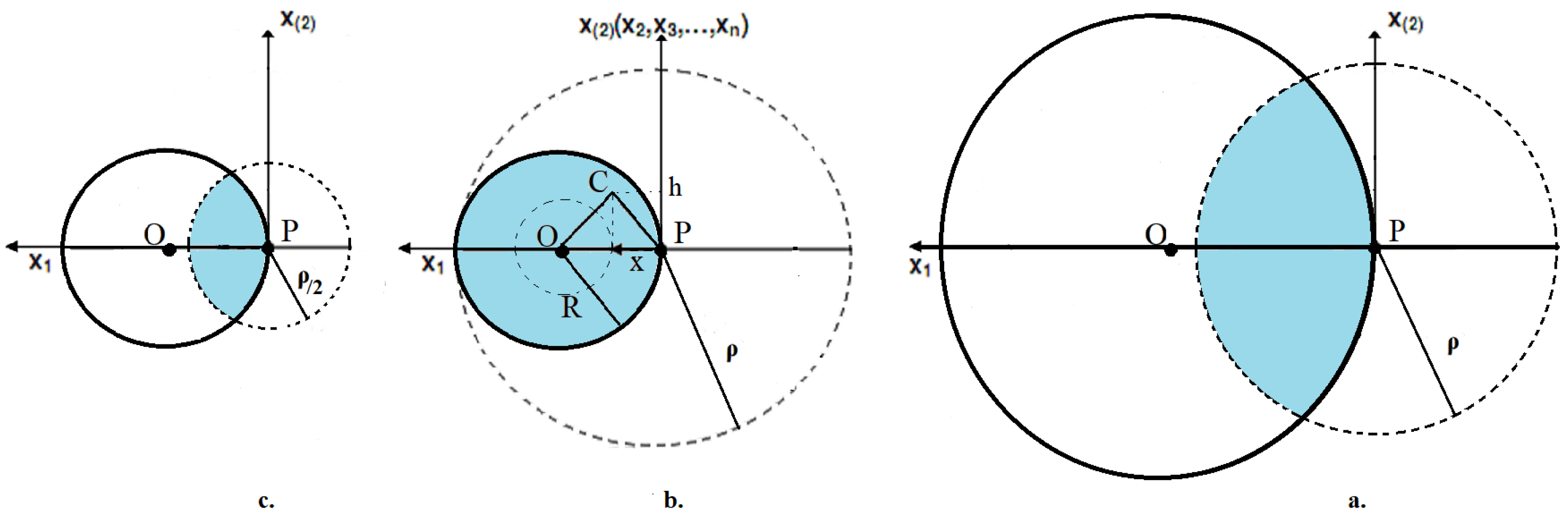
Under uniform mutation inside the sphere, the modification of the success region—and also the inhomogeneous Markov kernel—can be observed as the ES approaches the optimum in Figure 1, from right to left. In case (a), $R_x^S$ is the intersection of two spheres (corresponding to mutation and fitness). As the algorithm approaches the optimum, assuming $\rho$ has not changed, $R_x^S$ becomes a full (fitness) sphere, case (b). The ES stagnates at this point, the 1/5 rule is activated and $\rho$ is halved, such that $R_x^S$ becomes again the intersection of two spheres, case (c).

Among the many studies devoted to the convergence of elitist ES with the 1/5 success rule on SPHERE and similar quadratic fitness functions, we review in this paper only what we consider to be complete theories, which follow the general pattern presented in Algorithm 1 and also achieve proofs of global convergence. Consequently, we distinguish between classic ES theory, in Section 2, and general theories, in Section 3. In classic ES theory, the accent falls on local behavior, with global convergence being a consequence of the best-case local scenario. General theories, on the other hand, provide a unitary solution to the convergence paradigm. To classic ES theory we assimilate the works of Rechenberg, Schwefel, Beyer, Rudolph and Jägersküpper; and to general theories the analyses of Auger and Hansen of Akimoto, Auger and Glasmachers. Note that the papers of Jägersküpper fall somehow in between, since they build on local behavior, but also provide a global convergence proof outside the best-case local scenario. The adaptation mechanisms used in population-based ES—with multiple offspring, multiple parents and recombination, self-adaptation or covariance matrix adaptation—are briefly discussed as generalizations of the 1/5 success rule in Section 4.

We underline the fact that this review paper is not an exhaustive survey of the ES state-of-art—we defer to [25] for that purpose—but a personal reading of the convergence theories built in this field at the intersection of probability theory, computational complexity and statistics.

2. Classic ES Theory

As in Figure 1b, assume the algorithm and the center of the coordinate system are both in P; the distance to global optimum O is $R=\left|OP\right|$; denote $x_1$ by x and the remaining $n-1$ components $x_{\left(2\right)}$ by h. The classic ES theory focuses on the local, one-step behavior of the algorithm, where the mutation rate $\rho$ can be assumed constant.

If C is a random point generated by mutation, the progress becomes a one-dimensional r.v. corresponding to the difference in distance to optimum between the current ES position and the next. Due to the elitist selection, progress is non-negative. For a successful mutation, C is inside region $R_x^S$, the blue area in Figure 1. Apply Pythagoras to $OC$ and $u={\left|\right|h\left|\right|}^2$; then, progress becomes [10] and ([4], p. 54).

$$progress=\left|OP\right|-\left|OC\right|=R-\sqrt{{(R-x_1)}^2+\sum _{i=2}^n{x}_i^2}=R-\sqrt{{(R-x)}^2+u}.$$

(7)

Insert progress into the integral and set $A=R_x^S$; then Equations (6) and (7) build the so-called ES’ expected progress:

$$\varphi ={\int }_{R^S}\left(R-\sqrt{{(R-x)}^2+u}\right)f(x,u)dxdu.$$

(8)

In order to approximate the above integral, two distinct cases occur: (i) ES close to optimum, or large step size (Figure 1b); (ii) ES far from the optimum, or small step size (Figure 1a,c).

With the same uniform mutation distribution, ref. [24] refined the results of both [13,26], and came closer to the analysis reviewed below by considering, in the estimation of local expected progress, the same two cases. However, without a deeper insight into spherical distributions, the study yielded only upper bounds for the expected progress and thus lower bounds for the global convergence time. Additionally, [23] analyzed an EA with $\lambda >1$ individuals in the population, acting on the SPHERE, with uniform mutation inside the sphere. However, the analysis is confined to the case where optimum is within the mutation sphere—that means, large step size, for which only asymptotic ($\lambda \to \infty$) results are derived; again, a comparison to (32) is intractable. Noteworthy, yet again incomparable to the results reviewed below, are theoretical analyses of mutation distributions that are uniform but non-spherical [22,27].

2.1. Large Step Size

This case is defined by the inequality $\rho \ge 2R$, such that success region $R_x^S$ is completely included in the mutation sphere, Figure 1b. We assume uniform mutation inside the sphere, but an ES with normal mutation performs similarly, for large n and a proper parameter scaling [10,28].

Mathematically, this is the unique situation when Formula (8) is tractable, allowing for a closed-form derivation of the expected progress. However, the case did not receive much attention in the literature, since it corresponds to the worst case scenario (stagnation), calling for an emergency application of the mutation adaptation rule.

A first rigorous result concerning this case was provided by Rudolph, with the analysis of pure random search, an algorithm that generates offspring independently, using the uniform distribution inside the sphere with a fixed center and constant radius $\rho$ ([9], pp. 168–169). The minimal distance to optimum out of the first t trials, $R_t$, is computed, for large t, by order statistics [29]. The second approximation is with respect to large space dimension n.

$$R_t\approx \rho t^{-1/n}{\Gamma }_{1+\frac{1}{n}}\approx \rho t^{-1/n}.$$

(9)

The following definitions are used in computational complexity analysis [5,10].

Definition 2. 

• A statement $Z\left(n\right)$ holds for large enough n if there is $N\in \mathbb{N}$ such that for all $n\ge N$, $Z\left(n\right)$ holds.
• For $g\left(n\right)>0$, we say $g\left(n\right)=\mathcal{O}\left(n\right)$ if there exists $c>0$ such that $g\left(n\right)\le cn$, for a large enough n. Similarly, $g\left(n\right)=\Omega \left(n\right)$ if $g\left(n\right)\ge cn$, for a large enough n. If $g\left(n\right)$ is both $\mathcal{O}\left(n\right)$ and $\Omega \left(n\right)$, we say that $g\left(n\right)=\Theta \left(n\right)$.
• We say $g\left(n\right)=o\left(n\right)$ if $g\left(n\right)/n\to 0$ as $n\to \infty$.
• A sequence $p_n\ge 0$ is exponentially small in n if $p_n\le e^{-\mathcal{O}\left(n\right)}$.
• An event $A_n$ happens with overwhelming probability (w.o.p.) in n if $1-P\left(A_n\right)$ is exponentially small in n.

Rudolph argues that the convergence rate of elitist, constant mutation ES decreases to the asymptotics (9), estimated, after re-noting $R_t=ϵ$, as

$$t=\Theta \left[{\left(\frac{1}{ϵ}\right)}^n\right]$$

(10)

and classified as poor, compared to the performance of adaptive mutation ES.

One can note in Figure 1b that progress is minimal (zero) if the randomly generated point C is P and maximal (R) if the generated point is O. The success probability in the large step size case is simply the ratio of two n-sphere volumes, ${(R/\rho )}^n$. A complete description of the progress r.v. (7) is provided in the following.

Proposition 1. 

Assume the elitist ES with one individual and uniform mutation inside the sphere of radius ρ, minimizing the SPHERE, is at distance R from the origin, $\rho \ge 2R$. Then, the progress is

• cdf

  $$F\left(x\right)=P\left(R-\left|OC\right|\le x\right)=\left\{\begin{array}{cc}0,\hfill & x<0\hfill \\ 1-{\left(\frac{R}{\rho }\right)}^n,\hfill & x=0\hfill \\ 1-{\left(\frac{R-x}{\rho }\right)}^n,\hfill & x\in (0,R)\hfill \\ 1,\hfill & x\ge R\hfill \end{array}\right.$$

  (11)
• and partial pdf

  $$f\left(x\right)=\left\{\begin{array}{c}\frac{n}{{\rho }^n}{(R-x)}^{n-1},x\in (0,R)\hfill \\ 0,other\hfill \end{array}\right..$$

  (12)

Proof. 

It is easy to see that progress is non-negative, discontinuous and $P(progress=0)=1-{(R/\rho )}^n$. For $x\in (0,R)$, the point C can be seen as generated by the uniform distribution inside the sphere of radius $\rho$, but with center O. Then, $\left|OC\right|$ corresponds to $\mathbf{r}$, the radius of the uniform distribution inside the $\rho$-sphere, truncated to $S^O\left(R\right)$, the n-sphere with center O and radius R. Note the difference between the radius r.v. $\mathbf{r}$ from Definition 1, and the positive real number $\rho$, the radius of the mutation sphere.

However, $\mathbf{r}$ is $Beta(n,1)$ in the case of the uniform inside the sphere of radius $\rho$, with pdf [10]:

$$g\left(r\right)=\frac{1}{{\rho }^n}n{r}^{n-1},r\in (0,\rho ).$$

(13)

Restricted to $(0,R)$, the pdf (13) provides the (partial) cdf:

$$G\left(r\right)={\left(\frac{r}{\rho }\right)}^n,r\in (0,R),$$

(14)

such that

$$\begin{array}{cc}\hfill F\left(x\right)=& P(R-\mathbf{r}\le x)=1-P(\mathbf{r}\le R-x)=1-G(R-x)=\hfill \end{array}$$

(15)

$$\begin{array}{cc}\hfill =& 1-{\left(\frac{R-x}{\rho }\right)}^n,x\in (0,R).\hfill \end{array}$$

(16)

A simple derivation with respect to x provides the pdf (12). □

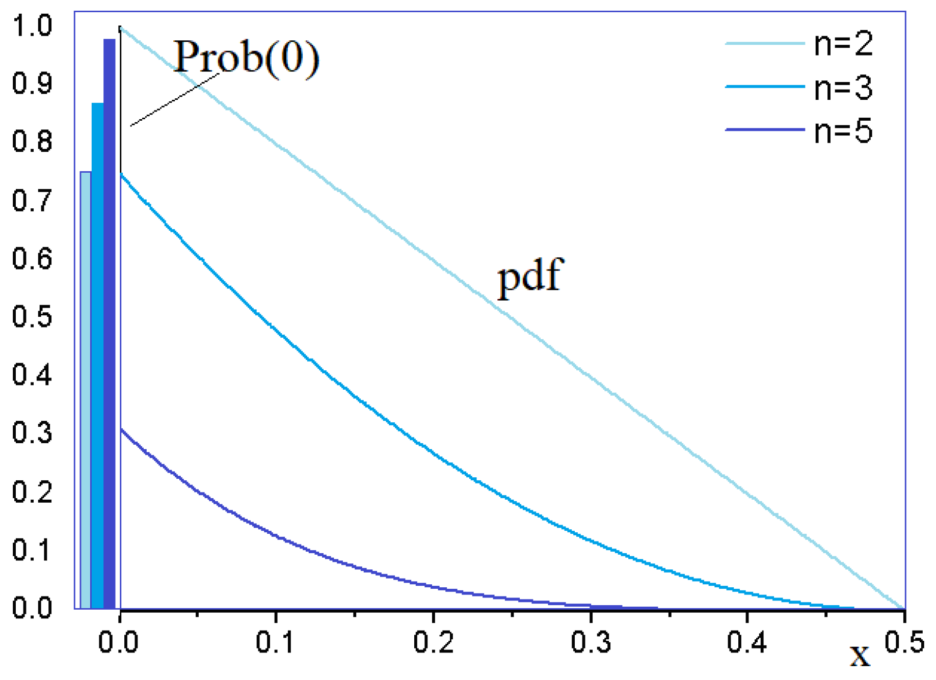
The progress r.v. is depicted in Figure 2, for $\rho =1,R=1/2$ and different space dimensions n. To each n corresponds a bar at zero—the Dirac measure ${\delta }_0$, that is, the discrete part of the progress—and a thin line with the same color representing the partial pdf of the continuous part of the progress.

The following result is a slight generalization of a similar result (on the particular case $\rho =1$) from [30]. However, the proof presented below is easier than the one in [30], building on the exact formulas provided by Proposition 1.

Theorem 1. 

In the conditions of Proposition 1,

• the success probability is

  $$P^S={\left(\frac{R}{\rho }\right)}^n,$$

  (17)
• the expected progress is

  $$\varphi =\frac{R^{n+1}}{{\rho }^n(n+1)}.$$

  (18)

Proof. 

The success probability has already been derived geometrically. However, in a unitary setting, both success probability and expected progress are obtained by integration of partial pdf (12) over the success region $(0,R)$.

$$\begin{array}{cc}\hfill & P^S={\int }_0^R\frac{n}{{\rho }^n}{(R-x)}^{n-1}dx={\left(\frac{R}{\rho }\right)}^n.\hfill \\ \hfill & \varphi =E\left(progress\right)={\int }_0^R\frac{nx}{{\rho }^n}{(R-x)}^{n-1}dx=\frac{R^{n+1}}{{\rho }^n(n+1)},\hfill \end{array}$$

where the second calculus yields from partial integration. □

Theorem 1 points out an outstanding analytical property of the uniform mutation operator, in case of the algorithm with a large step size: The success probability is the derivative, with respect to distance to optimum, of the expected progress.

This result relies on the non-centrality property of the uniform distribution inside the sphere. Namely, we can regard the random point C as being generated from a uniform centered in O, not in P, then apply the radius r.v. for the random distance $\left|OC\right|$. This procedure can be applied only for Figure 1b, not for Figure 1a or Figure 1c, and neither for other spherical mutation like the normal distribution. The uniform distribution on the sphere provides zero progress if $\rho \ge 2R$, so that case is also tractable but not interesting, corresponding to pure stagnation.

Finally, we confirm and generalize Rudolph’s result (10) on the convergence time of the elitist ES on the SPHERE, under constant, large-step-size mutation.

Theorem 2. 

In the conditions of Proposition 1, the time required by the algorithm to reach distance ϵ from optimum is

$$t=\Theta \left[{\left(\frac{\rho }{ϵ}\right)}^n\right].$$

(19)

Proof. 

Start from Equation (18) and the definition of progress (7).

$$\begin{array}{cc}\hfill \varphi =& \left|OP\right|-\left|OC\right|=R_t-R_{t+1}=\frac{R_t^{n+1}}{{\rho }^n(n+1)}\hfill \end{array}$$

(20)

$$\begin{array}{cc}\hfill & \Rightarrow R_{t+1}-R_t=-\frac{R_t^{n+1}}{{\rho }^n(n+1)}.\hfill \end{array}$$

(21)

We transform the above difference equation into a differential equation, with separable variables, which we solve.

$$\begin{array}{cc}\hfill y^{\prime }=& -\frac{y^{n+1}}{{\rho }^n(n+1)}\hfill \end{array}$$

(22)

$$\begin{array}{cc}\hfill & \Rightarrow \int \frac{y^{\prime }}{y^n}dy=-\int \frac{{\rho }^n}{n}dx\hfill \end{array}$$

(23)

$$\begin{array}{cc}\hfill & \Rightarrow y^{n-1}=\frac{n}{n-1}{x}^{-1}\hfill \end{array}$$

(24)

$$\begin{array}{cc}\hfill & \Rightarrow y={\left(\frac{n}{n-1}\right)}^{n-1}{\left(\frac{x}{{\rho }^n}\right)}^{-\frac{1}{n-1}}\approx x^{-\frac{1}{n}}\rho .\hfill \end{array}$$

(25)

At the last step, we remove the factors/exponents that converge to one as $n\to \infty$.

If we denote $y=R_t=ϵ$ and $x=t$, we get

$$ϵ\approx t^{-\frac{1}{n}}\rho \Rightarrow t\approx {\left(\frac{\rho }{ϵ}\right)}^n.$$

(26)

□

One should note that the relevance of the above analysis is purely theoretical. Inspection of Equations (17) and (18) shows that both success probability and expected progress attain their maximum for $\rho =2R$, where the two quantities are of order $1/2^n$, a rather low value, leading to stagnation. The situation is avoided in Algorithm 1 by halving $\rho$, such that the ES enters (again) the small step size situation of Figure 1c.

2.2. Small Step Size

This case is defined by the inequality $\rho <2R$, such that success region $R_x^S$ is the intersection of the mutation and fitness spheres; see Figure 1a,c.

If the ES uses uniform mutation inside the $\rho$-sphere, the following equation transforms the original radius into a new parameter, equivalent (asymptotically) to the standard deviation ($\sigma$) of the normal mutation [10,28].

$$a=\frac{\rho }{\sqrt{n}}.$$

(27)

Under the assumption $a\approx \sigma$, the local behavior of Algorithm 1 does not depend on the mutation distribution used: normal with standard deviation $\sigma$ or uniform inside the sphere of radius $\rho$—one can treat these two ES versions as one. Apply next a second normalization of both new mutation parameter a and expected progress $\varphi$ ([4], p. 32):

$$a^{*}=a\frac{n}{R},{\varphi }^{*}=\varphi \frac{n}{R}.$$

(28)

The random local behavior of the algorithm can be expressed by the following compact formulas ([4], pp. 67–68), [10]. The cumulative distribution function (cdf) of the standard normal (Gaussian) distribution $N(0,1)$ is $\Phi \left(x\right)=\frac{1}{\sqrt{2\pi }}{\int }_{-\infty }^x{e}^{-\frac{t^2}{2}}dt$.

Theorem 3. 

Let a elitist ES minimize the SPHERE, with either uniform mutation inside the sphere of radius ρ or normal mutation with standard deviation $a=\rho /\sqrt{n}$. Then, for large n, the following approximations hold:

• Success probability:

  $$Prob\approx 1-\Phi \left(\frac{a^{*}}{2}\right).$$

  (29)
• Normalized expected progress:

  $${\varphi }^{*}\approx \frac{a^{*}}{\sqrt{2\pi }}{e}^{-\frac{a^{*2}}{8}}-\frac{a^{*2}}{2}\left[1-\Phi \left(\frac{a^{*}}{2}\right)\right].$$

  (30)

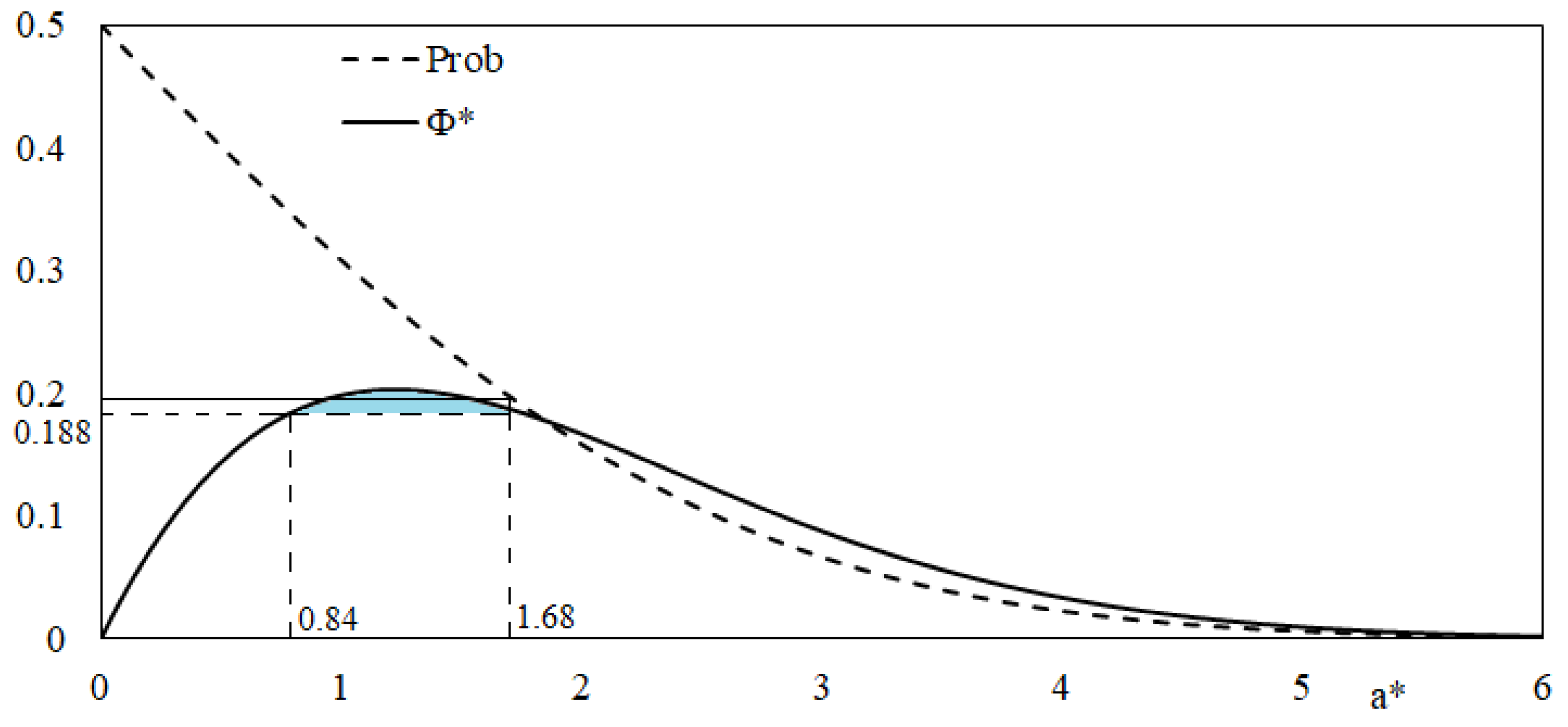
The asymptotics of success probability and expected progress are depicted in Figure 3. The particular form of ${\varphi }^{*}$ as function of $a^{*}$ is essential for proving the global convergence of the adaptive ES. Note that the function (30) is uni-modal, with a maximum at $a^{*}=1.224$, ${\varphi }_{\max }^{*}={\varphi }^{*}\left(1.22\right)=0.202$.

The blue area corresponding to the $a^{*}$-interval $[0.84,1.68]$ is the ‘evolution window’ of Algorithm 1. In classic ES theory, the term is used in the broader sense of the region with expected progress being significantly greater than zero, e.g., $a^{*}\in [0.1,5]$ in Figure 3 [1], ([4], p. 69), [31]. However, we use here the more restrictive definition from [10], which ensures also global convergence of the ES under the 1/5 rule. Using the success probability formula, Formula (29), we identify first the critical value $a^{*}=1.68$, corresponding to $Prob\left(1.68\right)=1/5=0.2$. Then, we apply the expected progress formula, Formula (30), get ${\varphi }^{*}\left(1.68\right)=0.188$ and use again (30) to get ${\varphi }^{*}\left(0.84\right)=0.188$. One could say that the evolution window in this case is defined by the condition ${\varphi }^{*}\ge 0.188$.

Observing the possible benefits of different mutation distributions, the authors of [3,9] developed an analysis based on uniform mutation on the sphere. Using the random angle $\theta =\angle CPO$ between the mutated point and the optimum direction, and the same parameter normalization, Rudolph solved the low-dimensional case, $n=3$. The general case proved intractable, so he resorted to the same approximation of a random variable through its expected value, yielding an asymptotic progress which is the double of Formula (30) ([9], pp. 170–172). Note that a different progress definition applies, usually referred to as quality gain:

$$\begin{array}{cc}\hfill & progres{s}^{\prime }=R^2-{\left|OC\right|}^2\hfill \end{array}$$

(31)

$$\begin{array}{cc}\hfill & {\varphi }^{\prime }=2{\varphi }^{*}.\hfill \end{array}$$

(32)

By applying another spherical mutation operator to the same problem, the Cauchy distribution, Rudolph obtained a different expression of progress, valid for the case $n=3$ [32]. Like the normal multivariate, the Cauchy distribution is with un-bounded support, can be constructed from independent identical components and exhibits the rare property of being closed to addition. Under quadratic definition (31), the expected progress ${\varphi }_C$ depends on the mutation parameter $\delta$:

$${\varphi }_C=1-\frac{1}{\delta \pi }\left[\frac{3}{\delta }arctan\left(2\delta \right)+\frac{2{\delta }^2-1}{2{\delta }^2}log(4{\delta }^2+1)-4\right].$$

(33)

Unfortunately, the generalization to larger dimensions failed, due to the intractability of radius $\mathbf{r}$ from Equation (2), in the case of the Cauchy distribution.

Considering yet another spherical distribution, the (averaged) sum of two independent uniforms inside the sphere, $\mathbf{x}=({\mathbf{x}}_1+{\mathbf{x}}_2)/2$ [10], also showed that ${\varphi }_S$, the expected progress of this new mutation operator, is

$${\varphi }_S\left(a^{*}\right)={\varphi }^{*}\left(\frac{a^{*}}{\sqrt{2}}\right).$$

(34)

Note that if ${\mathbf{x}}_{1,2}$ are uniformly distributed inside the sphere with radius $\rho$, the expected value of the radius r.v. $\mathbf{r}$ from Equation (1) is also $\rho$—asymptotically for large space dimension n. On the other hand, the expected value of the radius of $\mathbf{x}$ is $\rho /\sqrt{2}$, so the scaling factor of the argument in Equation (34) is actually the ratio between the different expected radiuses [10].

2.3. Global Convergence

For decades, the algorithm’s global convergence was only a marginal subject in classic ES theory, regarded as a consequence of the ability—un-explained theoretically, though supported by empirical evidence—of the 1/5 success rule to keep the expected progress around its maximal value during the whole evolution. We illustrate this with Beyer’s reasoning and apply Formula (30) to express the ES’s expected progress between time t and $t+1$ ([4], pp. 48–50).

$$\begin{array}{c}\hfill R_t-R_{t+1}=\varphi \left(a_t\right)\Rightarrow R_{t+1}-R_t=-R_t\frac{{\varphi }^{*}\left(a_t^{*}\right)}{n}.\end{array}$$

(35)

One obtains a separable differential equation from the difference equation.

$$R_t^{\prime }=-R_t\frac{{\varphi }^{*}\left(a_t^{*}\right)}{n}.$$

(36)

If the 1/5 rule manages to keep $a_t^{*}$ approximately constant at its maximum, ${\varphi }^{*}\left(a_t^{*}\right)\approx {\varphi }_{\max }^{*}=0.202$; the differential equation solves to the following (note that $R_0$ is the initial distance to optimum):

$$R_t=R_0{e}^{-\frac{0.202t}{n}}.$$

(37)

Apply next the logarithm to get

$$ln\left(\frac{R_t}{R_0}\right)=\frac{-0.202t}{n},$$

(38)

and then reverse Equation (38); denote $R_t=ϵ>0$ and $1/0.202=C$, such that

$$t=Cnlog\frac{R_0}{ϵ}.$$

(39)

According to Definition 2, Equation (39) reads as linear convergence time, with respect to both space dimension n and the logarithm of initial distance to optimum $R_0$. The only problem is that the above analysis is based on the optimistic assumption that the 1/5 rule keeps expected progress around the value of $0.202$. Rigorously, this is only a best-case scenario, so one should actually read the above equalities as inequalities and (39) as a lower bound on convergence time [10]. The ES convergence time is $\Omega \left[n·log\left(R_0/ϵ\right)\right]$.

$$t\ge Cnlog\frac{R_0}{ϵ}.$$

(40)

However, the practical efficiency of Equation (37), expressed by its ability in predicting the behavior of the real algorithm, is undeniable. Following [10], we present here another derivation of Formula (37) with a slightly different exponential parameter ($0.178$ instead of $0.202$) but obtained as an average, not extreme case value.

Rudolph considered first the stochastic nature of the ES, using a martingale model to derive sufficient conditions for global convergence. The following definitions and results are from ([9], pp. 25–26, 52, 166) and ([33], pp. 94, 109, 127–128, 131).

Definition 3. 

• The conditional expectation $E\left(R_{t+1}|R_t\right)$ is a r.v., with values $E\left(R_{t+1}|R_t=R\right)$ and probabilities of $R_t$, such that $E\left[E\left(R_{t+1}|R_t\right)\right]=E\left(R_{t+1}\right)$.
• A sequence of r.v.s ${\left\{R_t\right\}}_{t\in \mathbb{N}}$ is called

  –

  Non-negative supermartingale if, for all t,

  $$E\left(|R_t|\right)<\infty andE\left(R_{t+1}|R_t\right)\le R_t$$

  (41)

  –

  Uniformly integrable (UI) if, for any $ϵ>0$, there is $K\ge 0$ such that, for all t

  $$E\left(|R_t|·1_{\left\{\right|R_t|>K\}}\right)<ϵ.$$

  (42)

Proposition 2. 

Let ${\left\{R_t\right\}}_{t\in \mathbb{N}}$ be a sequence of r.v.s.

• A sufficient condition for UI is: there is $K>0$ such that $|R_t|<K$ for all t.
• If ${\left\{R_t\right\}}_{t\in \mathbb{N}}$ is a non-negative supermartingale, it converges a.s. to a finite r.v. If ${\left\{R_t\right\}}_{t\in \mathbb{N}}$ is also UI, convergence is also in the mean.

Let $X_t$ be the r.v. elitist ES at iteration t, f a function with minimum zero and $R_t=f\left(X_t\right)$. Then, ${\left\{R_t\right\}}_{t\in \mathbb{N}}$ is a non-negative supermartingale due to the elitist selection, and UI since $R_t\le R_0$. Due to Proposition 2, $R_t$ converges a.s. and in mean to a finite r.v. What remains to be proved is:

• Global convergence—the limit is exactly zero;
• Convergence rates.

Sufficient convergence conditions are provided in ([9], pp. 165–167). Note that part (a) of Theorem 4 is also presented in [34], and part (b), in terms of dynamical systems and Lyapunov functions, is also in ([15], p. 154).

Theorem 4. 

Let ${\left\{X\right\}}_{t\in \mathbb{N}}$ be generated by some ES optimizing a fitness function f with global minimum at zero, and $R_t=f\left(X_t\right)>0$.

(a) 

If the ES employs an elitist selection rule and there exist sequences ${ϵ}_t,{\delta }_t\in (0,1)$ such that for all t

$${\delta }_t\le Prob\left\{R_{t+1}\le (1-{ϵ}_t)R_t|R_t\right\}$$

(43)

and

$$\sum _{t=0}^{\infty }{ϵ}_t·{\delta }_t=\infty$$

(44)

then the ES converges to zero a.s and in mean, and the approach is exponentially fast with rate $c=1-\delta ·ϵ\in (0,1)$.

$$E_{R_{t+1}}\le E_{R_t}c\Rightarrow E_{R_t}\le E_{R_0}{c}^t.$$

(45)

(b) 

Regardless of the selection rule, if there is a constant $c\in (0,1)$ such that for all t

$$E\left(R_{t+1}|R_t\right)\le c·R_{t}a.s.$$

(46)

then the ES converges to zero a.s. and in mean, and the approach is exponentially fast with rate c.

The key r.v.s and parameters used in this study are summarized in

Table 1. Mathematical concepts used in ES analysis.

$X_t$	n-dim r.v. ’ES position at time t’
$R_t$	1-dim r.v. ’ES distance to optimum at time t’
R	positive real number
$\left(R_{t+1}|R_t=R\right)$	1-dim r.v. ’ES distance to optimum
	at $t+1$, conditioned by dist. R at t’
$E\left(R_{t+1}|R_t=R\right)$	positive real number, mean of the above
$E\left(R_{t+1}|R_t\right)$	1-dim r.v. ’ES distance to optimum
	at $t+1$, conditioned by distance at t’
${\varphi }_t(R,n,\rho )=R-$	non-negative real number, mean
$-E\left(R_{t+1}|R_t=R\right)$	progress between time t and $t+1$
${\varphi }_t^{*}\left(a^{*}\right)={\varphi }_{t}n/R$	non-negative real number,
	normalized mean progress
$T_d$	1-dim r.v. ’first hitting time of distance d’

.

Rudolph used Theorem 4 (b) to justify global convergence on SPHERE, for the elitist ES with uniform mutation on sphere ([9], pp. 170–172). However, the reasoning is unrealistic: it assumes a mutation radius proportional, at each moment, to distance to the optimum of ${\rho }_t=\gamma R_t$, with the parameter set to optimal value ${\gamma }^{*}=1.224$.

The problem is that a real ES, modeled as a sequence of (decreasing) constant-mutation phases, delimited by the application of the 1/5 rule, does not fulfill Equations (43)–(46) per se. Assuming a ’good’ starting point (see Theorem 7), there is a constant $c>0$ such that (46) holds as long as the ES is within some narrow evolution window, such as the one depicted in Figure 3. However, as the algorithm reaches the upper limit of the evolution window, at some random time T, there is an exponentially small probability for the ES to continue the descent such that (46) is precluded. Since mutation adaptation is necessary for global convergence, we are interested in the (large probability) event ‘the 1/5 rule applies at iteration T’. The situation resembles Theorem 4 (a), with the difference being that $E\left(R_{T+1}|R_T\right)=R_T$ for the 1/5 rule applies only in unsuccessful iterations, such that ${ϵ}_T=0$ and (43) is precluded as well.

Summing up, Theorem 4 is not strong enough to derive upper bounds on the global convergence time of the elitist ES with the 1/5 success rule. As one can see in the following, the mathematical difficulty resides not in the multi-variate calculus, but in the computational complexity analysis of the 1/5 rule. The linear upper bounds were proved for the first time by Jägersküpper, who regarded the elitist ES as a sequence of n-length phases with a constant mutation rate in each phase, during which the success frequency of mutation was observed before the application of the 1/5 rule [5,26,35,36].

Removing line (ii) from the 1/5 rule in Algorithm 1—that is, parameter $\rho$ decreases if success frequency is less than 1/5, but never increases—and using A uniform mutation inside the sphere instead of normal mutation, [10] proved that all of Jägersküpper’s results still hold. Moreover, under the simplified 1/5 rule, the constant-mutation phase extends to a number of phases, called a cycle. The r.v. ’length of a cycle’ will play a key role in connecting the two (otherwise distinct) parts of the convergence analysis, local and global, leading to an exponential formula able to predict the behavior of the real ES, similar to Equation (37).

We resume next the results from [5,10,26,35,36] in a unitary setting, covering both types of 1/5 rule and both mutation distributions, normal and uniform inside the sphere. The results hold also for the sum of two uniforms; see [10] for details. For the local behavior, Jägersküpper avoided the calculus from Section 2.2 and used instead the decomposition (2) of the normal mutation distribution with standard deviation $\sigma$, $N(0,\sigma I_n)$, into r.v.s uniform on sphere ${\mathbf{u}}^{\mathbf{n}}$ and radius ℓ. Recall that $\rho$ is the radius parameter of the uniform mutation inside the sphere, R the current distance to optimum, $Prob$ the success probability and $\mathbf{r}$ the radius r.v. from Equation (1). We also apply the normalization $a=\rho /\sqrt{n}$ in order to equalize the asymptotic mean radiuses of the two distributions, normal and uniform, such that a can be identified to $\sigma$ and $\mathbf{r}$ to ℓ.

Lemma 1. 

Let Algorithm 1 with any spherical mutation minimizing the SPHERE be in current point P; $\left|OP\right|=R$. The mutant C is accepted with $Prob\in [ϵ,1/2-ϵ]$, $ϵ>0$, if and only if $\left|PC\right|=\Theta \left(R/\sqrt{n}\right)$.

Lemma 2. 

If X is uniform inside the sphere of radius ρ or normal with standard deviation $\sigma =\rho /\sqrt{n}$, and $\mathbf{r}$ is the corresponding r.v. radius, then

$$P\left(|\mathbf{r}-\rho |\le \delta \rho \right)\ge 1-\mathcal{O}\left(\frac{1}{n{\delta }^2}\right).$$

(47)

If $X_1,\dots ,X_n$ are independent copies of X, then for any $\lambda \in (0,1)$, there exist $a_{\lambda },b_{\lambda }>0$ such that the r.v. cardinal number of $\left\{i|a_{\lambda }\rho \le r_i\le b_{\lambda }\rho \right\}$ is $\ge \lambda n$ w.o.p.

The first part of Lemma 2 is actually Chebyshev inequality. Note that the inequality $|\mathbf{r}-\rho |\le \delta \rho$ is equivalent to $|\mathbf{r}-\rho |/\rho \le \delta$, so the result holds for the original (that is, before normalization $\rho =a\sqrt{n}$) uniform distribution inside the sphere, for the normalized uniform and also for the normal distribution.

Lemma 3. 

Let Algorithm 1 with mutation X, as in Lemma 2, minimize the SPHERE. The following are equivalent:

(i) 

$\sigma =\Theta \left(R/n\right)$

(ii) 

$\rho =\Theta \left(R/\sqrt{n}\right)$

(iii) 

There exists $ϵ>0$ such that $Prob\in \left[ϵ,\frac{1}{2}-ϵ\right]$ for a large enough n—that is, $Prob$ is $\Omega \left(1\right)$ and $1/2-\Omega \left(1\right)$.

Lemma 4. 

If $\mathbf{r}=\Theta \left(R/\sqrt{n}\right)$, then progress is $\Theta \left(R/n\right)$, with probability $\Omega \left(1\right)$, and within expectation.

The radius $\mathbf{r}$ in Lemma 4 corresponds to the normalized ($\rho =a\sqrt{n}$) uniform inside the sphere, and hence also to the normal distribution.

Let $i,i+1$ denote the states of the algorithm at the beginning/end of this phase, respectively.

Lemma 5. 

Let Algorithm 1 with mutation X as in Lemma 2 minimize the SPHERE. Consider two variants of the 1/5 rule: (i and ii).

(i) 

If ${\rho }_i=\Theta \left(R_i/\sqrt{n}\right)$, then $R_i-R_{i+1}=\Theta \left(R_i\right)$ w.o.p.; that is, w.o.p. the approximation error is reduced by a constant fraction in the i-th phase.

(ii) 

If ${\rho }_i$ is doubled (or respectively not modified) after the i-th phase, then ${\rho }_i=\mathcal{O}\left(R_i/\sqrt{n}\right)$.

(iii) 

If ${\rho }_i$ is halved after the i-th phase, then ${\rho }_{i+1}=\Omega \left(R_{i+1}/\sqrt{n}\right)$.

Lemma 6. 

Let Algorithm 1 be as in Lemma 5. If the 1/5 rule causes a $(k+1)$-sequence of phases, $1\le k=n^{\mathcal{O}\left(n\right)}$, such that in the first phase ρ is halved and in all the following it is doubled (respectively left unchanged), or the other way around, then w.o.p. the distance from optimum is k times reduced by a constant fraction in these phases.

We can state now the main global convergence result, valid for the ES with either uniform or normal mutation, with either complete (i–ii) or simplified (i) 1/5 success rule [5,10,35].

Theorem 5. 

Let Algorithm 1, defined as in Lemma 5, start at distance $R_0$ from optimum, with mutation parameter ${\rho }_0=\Theta \left(R_0/\sqrt{n}\right)$. If t satisfies $1\le t=n^{\mathcal{O}\left(1\right)}$, then the number of iterations to reach distance $R_t$ with $R_t\le R_0/2^t$ is $\Theta (t·n)$, w.o.p. and within expectation.

For $t=1$, Theorem 5 states the existence of two constants $a,b>0$, such that for a large enough n, the random time T required to halve the initial distance to optimum $R_0$ satisfies

$$an\le E\left(T\right)\le bn.$$

(48)

Even if the result does not state convergence to zero of r.v. $R_t$, as $t\to \infty$, neither in expectation, nor a.s. nor w.o.p., it accounts for a form of linear convergence, with respect to both t and n.

Remark 1. 

For an arbitrary initial point, outside the prescribed range ${\rho }_0=\Theta \left(R_0/\sqrt{n}\right)$, Jägersküpper conjectured in [35] that: ‘For other starting conditions, the number of steps until the theorem’s assumption is met must be estimated before the theorem can be applied—by estimating the number of steps until the scaling factor is halved at least once. This is a rather simple task when utilizing the strong results presented in Lemma 5’. Empirical evidence for this fact can be found in [10].

This is the point where Jägersküpper’s convergence time analysis stops, without providing a formula similar to (37), to be tested against the behavior of the real ES. To fill in the gap, reference [10] applied the uniform mutation inside the sphere and the simplified 1/5 rule—obtained by removing line (ii) from Algorithm 1—and made use of the r.v. T = ‘length of a constant-mutation ES cycle’, defined as a stopping time ([33], pp. 97–98).

Definition 4. 

A r.v. T with state space $\{0,1,\dots ,\infty \}$ is said to be a stopping time for the sequence of r.v.s ${\left\{X_t\right\}}_{t\in \mathbb{N}}$ if one can decide whether the event $\{T=t\}$ has occurred only by observing $X_1,\dots ,X_t$. Note that, since the ES is a Markov chain, we do not assume independence of $X_1,X_2,\dots$, as in Wald’s equation and renewal theory [37].

Stopping time will be considered the first hitting time of distance $d>0$ from the initial point $X_0$.

$$T_d=min\left\{t\right|X_1+\dots +X_t\ge d\}.$$

(49)

A key role in the analysis is played by the following generalization of Wald’s equation ([37], p. 38), as introduced in [10]. Note that we define, for some r.v. X and $P\left(A\right)>0$, the conditional expectation $E\left(X|A\right)=E\left(X·{\mathbf{1}}_A\right)/P\left(A\right)$.

Proposition 3 

(Wald’s inequality [10]). Let $c,d,{\delta }_{\ell },{\delta }_u>0$ and ${\left\{X_t\right\}}_{t\in \mathbb{N}}$ be non-negative r.v.s such that $X_0=c$ and ${\delta }_{\ell }\le E\left(X_t|T_d\ge t\right)\le {\delta }_u$ for $t\ge 1$. Then

$$\frac{d}{{\delta }_u}\le E\left(T_d\right)\le \frac{d+{\delta }_u}{{\delta }_{\ell }}.$$

(50)

We set in our ES analysis $X_0=c=R_0>d$ and $X_{t+1}=R_t-R_{t+1}$; hence, $X_1+\dots +X_t=R_0-R_t$ for all $t\ge 0$.

Another form of Wald’s inequality can be obtained from the additive drift theorem, derived by Lehre and Witt in [38]—which, as the authors mention, adapts for the continuous case the discrete space drift theorem of He and Yao [14]. We apply a formalization similar to Proposition 3.

Theorem 6 

(Additive Drift). Let ${\left\{X_t\right\}}_{t\in \mathbb{N}}$ be a stochastic process, adapted to a filtration ${\left\{{\mathcal{F}}_t\right\}}_{t\in \mathbb{N}}$, over some state space $S\subseteq \Re$; let $d,{\delta }_{\ell },{\delta }_u>0$ and $T_0=min\left\{t\right|X_t>0\}$. Then, if $0\le X_t\le d=X_0$ and ${\delta }_{\ell }\le E\left(X_t-X_{t+1};X_t>0|{\mathcal{F}}_t\right)\le {\delta }_u$ for all t

$$\frac{d}{{\delta }_u}\le E\left(T_0|{\mathcal{F}}_0\right)\le \frac{d}{{\delta }_{\ell }}.$$

(51)

To be comparable with Wald’s inequality, one should set $X_{t+1}=d-(R_0-R_{t+1})$ in the Adaptive Drift theorem. However, we consider the assumption $X_t\ge 0$ for all t, implying $X_{T_d}=0$, to be unrealistic for $d<R_0$. On the other hand, if one sets $d=R_0$ as above, the lower bound ${\delta }_{\ell }>0$ does not exist (independent of t) in the continuous case, e.g., the SPHERE. The existence of a strictly positive lower bound on either success probability or expected progress can be seen as a sufficient convergence condition for continuous space algorithms—see also Theorem 4—yet it is only satisfied in discrete space.

Back to the application of Wald’s inequality in deriving convergence rates for the ES model. Let n be arbitrarily fixed; $d<R_0$; and consider the two $a^{*}$-values corresponding to the lower and upper limits of the evolution window depicted in Figure 3, $a_1^{*}=0.84$ and $a_2^{*}=1.68$. The normalized distance $d^{*}$ between these points corresponds to the un-normalized distance

$$d=R_{0.84}-R_{1.68}=\rho \sqrt{n}\left(\frac{1}{0.84}-\frac{1}{1.68}\right),$$

(52)

which further leads, using Wald’s inequality (see [10] for details), to

Theorem 7. 

Let Algorithm 1 be as in Theorem 5, starting in point $a^{*}=0.84$, and let $d^{*}=1.68-0.84$. Then, for large n

$$2.5n\le E\left(T_d\right)\lesssim 5.3n.$$

(53)

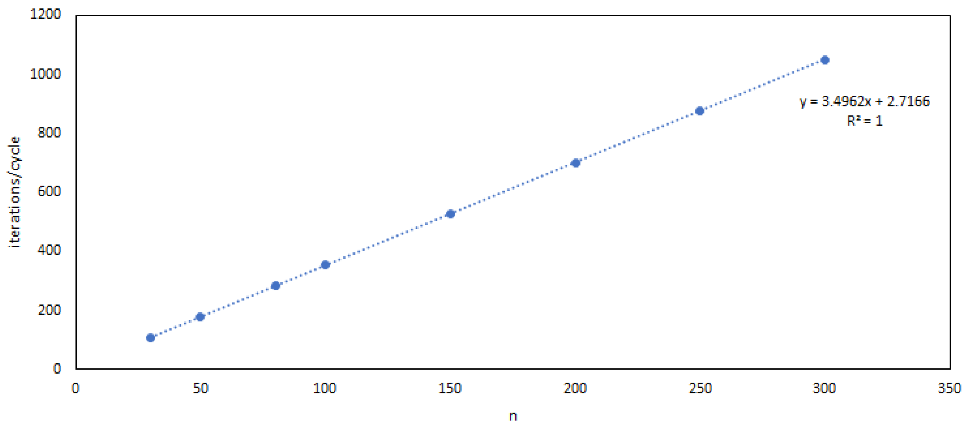
The resemblance between Equations (48) and (53) is obvious. According to Theorem 7, if the elitist ES is currently (initially) in point $a_0^{*}=0.84=\rho \sqrt{n}/R_0$, the expected time to reach $2a_0^{*}=1.68=\rho \sqrt{n}/(R_0/2)$ is within $[2.5n,5.3n]$. One could use these limits as lower and upper bounds on $E\left(T\right)$, or search for some value in between, to be used as an estimate for $E\left(T\right)$. In [10] the simple arithmetical mean $3.9$ has been used, yet we choose here the estimate $3.5$, as suggested by the new empirical evidence presented in Figure 4. The experiments were conducted with Algorithm 1 and uniform mutation inside the sphere, on the SPHERE fitness function, with different space dimensions and initial points, all corresponding to $a^{*}=0.84$. The results were averaged over 100 independent runs. In each run, the maximal number of iterations was set to $t_{max}=\mathrm{50,000}$, and the last, incomplete cycle was discarded.

Using the value $3.5$ for the expected value estimate of the r.v. T = ‘No. of iterations per constant-mutation ES cycle’, we obtained

$$R_{3.5n}\approx \frac{R_0}{2}.$$

(54)

By iterating Equation (54) s times and substituting in $3.9ns=t$, we get

$$R_{3.5ns}=\frac{R_0}{2^s}\Rightarrow R_t=R_0{2}^{-\frac{t}{3.5n}},$$

(55)

which further implies, with $log2/3.5=0.192$,

$$R_t=R_0{e}^{-\frac{0.192t}{n}}.$$

(56)

Using $R_t=ϵ$ and a derivation similar to the one inferred from Equation (37), the linear convergence of the elitist ES on SPHERE is finally obtained.

$$\mathrm{elitist}\mathrm{ES}\mathrm{convergence}\mathrm{time}=\Theta \left(n·log\frac{R_0}{ϵ}\right).$$

As demonstrated in [10], Formula (56) can be used, with very good experimental results, as a theoretical predictor of the algorithm’s global behavior. Note that the slightly different exponential coefficient, $0.192$ instead of $0.178$ in [10], is not disruptive.

On the other hand, the above model, indicating identical behavior of the elitist ES within each constant mutation cycle, offers an intuitive insight into the algorithm’s dynamics, seen as a sequence of cycles, that are independent and with identical expected length.

3. General 1/5-Rule Theories

Different convergence theories for the elitist ES with 1/5 success rule exist, building up mathematical rigor and complexity, yet, by imposing supplementary conditions, they usually lack compact results such as Theorem 3 and Formula (56). Some relevant examples are reviewed in the following.

Rudolph’s stochastic analysis based on martingales, presented already in Section 2.3, provides only sufficient global convergence conditions for the algorithm. A different stochastic process—a random system with complete connections—was used with a similar outcome in [16]. With a deeper insight into the theory of the irreducible Markov chain, which identifies the discrete states to the so-called small sets and extrapolates the basic features of a discrete homogeneous Markov chain onto the continuous space [39,40], Dorea proved, under elitist selection, the global convergence of ES and of a continuous version of simulated annealing to an $ϵ$-vicinity of the optimum [17]. However, since the mutation distribution is decoupled from the current position, the result is of little practical use. Bienvenüe and Francois applied a different Markov model to an adaptive ES, but under a different, problem-related adaptation rule that multiplies at each iteration the mutation parameter $\rho$ with the current distance to optimum $R_t$, then searches for ’optimal universal step lengths on the basis of the convergence of the dynamics’ [41]. The same adaptation rule was used by Rudolph in his convergence analysis of the elitist ES on SPHERE ([9], p. 70). Connecting the mutation rate to the current position works for the SPHERE centered on the origin, but failed for a slightly modified problem, e.g., for a SPHERE with a different center—where Algorithm 1, adapting the mutation rate according to the 1/5 rule, works very well.

Unaware of Dorea’s work, Auger and Hansen re-iterated the irreducible Markov chain modeling, but on the more practical premises used by Jägersküpper [2,18]. Similarly to Bienvenüe and Francois, but without their over-simplifying assumption, Auger and Hansen achieved, at the mathematical peak of ES literature, linear convergence of the elitist ES with the 1/5 rule on scaling-invariant functions (SPHERE included) by studying the stability of the normalized Markov chain $Z_t=R_t/\sigma$ [19]. A compact formula similar to (56) was proved.

$$R_t=R_0{e}^{-CRt},$$

(57)

where $CR>0$ depends on the asymptotic success probability $PS$ and on the 1/5 rule parameters $\gamma ,q$.

$$\left\{\begin{array}{cc}\hfill & CR=-ln\gamma \left(\frac{q+1}{q}PS-\frac{1}{q}\right)\hfill \\ \hfill & \mathrm{increasing}1/5\mathrm{rule}\mathrm{factor}\gamma \hfill \\ \hfill & \mathrm{decreasing}1/5\mathrm{rule}\mathrm{factor}{\gamma }^{-1/q}.\hfill \end{array}\right.$$

(58)

A supplementary condition is imposed on the parameters, which reads for the SPHERE

$$\frac{1}{2}\left(\frac{1}{\gamma }+{\gamma }^{\frac{1}{q}}\right)<1.$$

(59)

Bringing some clarity and a new stochastic formalization to the previous approach, Akimoto, Auger and co-workers employed drift analysis to prove the linear convergence time [6,11,42]. However, since their theory is still avoiding the expected progress calculus, a verification against the behavior of real algorithms can be performed only in terms of upper and lower bounds—see also the critique of adaptive drift theorem from Section 2.3.

4. Extensions of the 1/5-Rule—Population-Based ES

As noticed from the very beginning, the ES performance depends strongly on the value of the mutation parameter $\sigma$ (or $\rho$). The 1/5 success rule discussed so far is the simplest, yet not the only way of adapting the parameter during the algorithm’s evolution. Two of the most efficient techniques are the $\sigma$-self-adaptation [1,4,8] and the covariance matrix adaptation (CMA), which allows for different $\sigma$-values on the independent components (of normal mutation), aiming at accelerating the evolution in certain directions of the n-dimensional space [12,25,43,44].

As Beyer pointed out, each of these popular adaptation techniques borrows something from the original 1/5 success rule. The CMA techniques ’have an operating mechanism similar to the 1/5 rule: they analyze the statistical features of the selected mutations in order to change the strategy parameters towards the optimal value’ ([4], p. 258). Namely, the pdf of multivariate normal mutation in CMA-ES is

$$f\left(\mathbf{x}\right)=\frac{1}{{\left(\sqrt{2\pi }\right)}^n\sqrt{det\left(C\right)}}{e}^{-\frac{{\mathbf{x}}^T{C}^{-1}\mathbf{x}}{2}}$$

(60)

with symmetric covariance matrix C depending on $n(n+1)/2$ mutation parameters. If one considers all these parameters as independent r.v.s and switches from a single to a multiple offspring algorithm—one parent, $\lambda$ offspring and no elitist selection being the simplest case, known as $(1,\lambda )$ ES—Rudolph argues that a very large number of individuals is required in order to obtain a good approximation of the optimal matrix C. Pointing out that, in case of quadratic-convex fitness functions, the optimal C is the inverse of the function’s Hessian matrix, he suggests that the CMA update rules should follow the deterministic iterative methods of approximating the Hessian matrix, based on the information gathered from previous samples ([9], p. 198); see also [43]. According to the recent survey of the state-of-art in ES for continuous optimization [25], ‘we still lack a rigorous analysis of the one-step approximation of the covariance matrix’.

As a general remark in case of population-based algorithms—with multiple offspring, as for the $(1,\lambda )$ ES discussed above or the $(\mu /\mu ,\lambda )$ ES with multiple parents, offspring and recombination/crossover [45,46], the explicit reduction of the mutation parameter induced by the 1/5 success rule is not necessary anymore, its exploitation effect being accomplished by the (minimum) order statistics of the $\lambda$ offspring sample and/or by the $\mu /\mu$ recombination of the parent population. Intuitively, the explanation is provided by the following fact: The average of two multivariate uniform distributions inside the sphere of radius $\rho$ is also spherical, but with a smaller (expected value) radius, $\rho /\sqrt{2}$ instead of $\rho$; see [28] for details.

On the other hand, in self-adaptation, the dynamics of the mutation parameter is not based on some success-related statistics, but included in the evolution itself, subject to the basic algorithmic operators. Since mutation parameter $\sigma$ becomes in this case part of the individual, ‘the question reduces to the manner in which $\sigma$ should be mutated. The answer is: multiplicatively, in contrast to the additive mutations of object parameters’ ([4], p. 259). Obviously, the multiplicative character of the adaptation is inspired by the 1/5 rule.

5. Conclusions

Using the elitist, single-individual algorithm with mutation and the 1/5 success rule as the adaptation procedure and the SPHERE fitness function, the paper provides a bird eye’s view over the theory of evolution strategies, an important class of probabilistic optimization algorithms for multi-dimensional real space.

Despite their easy implementation and huge success in applications, the mathematical models are complicated, and global convergence results are rather scarce. Taking into account some recent studies applying the uniform distribution inside the sphere as a mutation operator, the review centered on the classic evolution strategy theory, built on the one-step behavior of the algorithm and on local quantities such as success probability and expected progress. For the first time in the literature, the three main building blocks of classic theory were presented together in a coherent formalization:

• the asymptotic (w.r.t. large space dimension) local expected progress formula,
• the computational complexity analysis proving lower and upper linear bounds for global convergence,
• a probabilistic analysis—using an adaptation of Wald’s equation—of the cyclic behavior of the algorithm with constant mutation rate, connecting the local and global behavior into a prediction formula for the (expected) convergence time of the real algorithm.

Different theories, based on martingales, irreducible Markov chain and drift analysis, were also reviewed, and their results were compared with those of classic theory.

As for population based algorithms—$(1,\lambda )$, $(\mu /\mu ,\lambda )$, CMA and self-adaptive ES—the role of the 1/5 rule is transferred to the selection and crossover operators, yielding a reduction in the mutation parameter for local improvement.

Since the 1/5 rule is devoted to exploitation, not to the exploration phase of the algorithm, the case of multi-modal fitness functions was not tackled in this paper.

References

- Rechenberg, I. Evolutionsstrategie: Optimierung Technischer Systeme nach Prinzipien der Biologischen Evolution; Frommann-Holzboog Verlag: Stuttgart, Germany, 1973. [Google Scholar]
- Auger, A. Convergence results for the (1,λ)-SA-ES using the theory of ϕ-irreducible Markov chains. Theor. Comput. Sci. 2005, 334, 35–69. [Google Scholar] [CrossRef] [Green Version]
- Schumer, M.A.; Steiglitz, K. Adaptive Step Size Random Search. IEEE Trans. Aut. Control 1968, 13, 270–276. [Google Scholar] [CrossRef] [Green Version]
- Beyer, H.-G. The Theory of Evolution Strategies; Springer: Berlin/Heidelberg, Germany, 2001. [Google Scholar]
- Jägersküpper, J. How the elitist ES using isotropic mutations minimizes positive definite quadratic forms. Theor. Comp. Sci. 2006, 361, 38–56. [Google Scholar] [CrossRef] [Green Version]
- Akimoto, Y.; Auger, A.; Glasmachers, T. Drift theory in continuous search spaces: Expected hitting time of the (1 + 1)-ES with 1/5 success rule. In Proceedings of the GECCO ’18: Genetic and Evolutionary Computation Conference, Kyoto Japan, 15–19 July 2018; pp. 801–808. [Google Scholar]
- Fang, K.-T.; Kotz, S.; Ng, K.-W. Symmetric Multivariate and Related Distributions; Chapman and Hall: London, UK, 1990. [Google Scholar]
- Schwefel, H.-P. Evolution and Optimum Seeking; Wiley: New York, NY, USA, 1995. [Google Scholar]
- Rudolph, G. Convergence Properties of Evolutionary Algorithms; Kovać: Hamburg, Germany, 1997. [Google Scholar]
- Agapie, A.; Solomon, O.; Bădin, L. Theory of (1+1) ES on SPHERE revisited. IEEE Trans. Evol. Comp. 2022. [CrossRef]
- Akimoto, Y.; Auger, A.; Glasmachers, T.; Morinaga, D. Global Linear Convergence of Evolution Strategies on more than Smooth Strongly Convex Functions. SIAM J. Optim. 2020, 32, 1402–1429. [Google Scholar] [CrossRef]
- He, X.; Zheng, Z.; Zhou, Y. MMES: Mixture Model-Based Evolution Strategy for Large-Scale Optimization. IEEE Trans. Evol. Comp. 2021, 25, 320–333. [Google Scholar] [CrossRef]
- Agapie, A.; Agapie, M.; Rudolph, G.; Zbaganu, G. Convergence of evolutionary algorithms on the n-dimensional continuous space. IEEE Trans. Cybern. 2013, 43, 1462–1472. [Google Scholar] [CrossRef]
- He, J.; Yao, X. A study of drift analysis for estimating computation time of evolutionary algorithms. Nat. Comput. 2004, 3, 21–35. [Google Scholar] [CrossRef]
- Rudolph, G. Stochastic Convergence. In Handbook of Natural Computing; Rozenberg, G., Bäck, T., Kok, J., Eds.; Springer: Berlin/Heidelberg, Germany, 2013; pp. 847–869. [Google Scholar]
- Agapie, A. Theoretical analysis of mutation-adaptive evolutionary algorithms. Evol. Comput. 2001, 9, 127–146. [Google Scholar] [CrossRef]
- Dorea, C.C. Stationary Distribution of Markov Chains in Rd with Application to Global Random Optimization. Bernoulli 1997, 3, 415–427. [Google Scholar] [CrossRef]
- Auger, A.; Hansen, N. Linear Convergence of Comparison-based Step-size Adaptive Randomized Search via Stability of Markov Chains. SIAM J. Optim. 2016, 26, 1589–1624. [Google Scholar] [CrossRef] [Green Version]
- Auger, A.; Hansen, N. Linear Convergence on Positively Homogeneous Functions of a Comparison-based Step-size Adaptive Randomized Search: The Elitist ES with Generalized One-fifth Success Rule. arXiv 2013, arXiv:1310.8397. [Google Scholar]
- Haario, H.; Saksman, E. Simulated Annealing Process in General State Space. Adv. Appl. Prob. 1991, 23, 866–893. [Google Scholar] [CrossRef]
- Vose, M.D. The Simple Genetic Algorithm: Foundations and Theory; MIT Press: Cambridge, MA, USA, 1999. [Google Scholar]
- Chen, Y.; He, J. Average convergence rate of evolutionary algorithms in continuous optimization. Inf. Sci. 2021, 562, 200–219. [Google Scholar] [CrossRef]
- Meunier, L.; Chevaleyre, Y.; Rapin, J.; Royer, C.W.; Teytaud, O. On Averaging the Best Samples in Evolutionary Computation. In Parallel Problem Solving from Nature—PPSN XVI: 16th International Conference, PPSN 2020, Leiden, The Netherlands, 5–9 September 2020, Bäck, T., Preuss, M., Deutz, A., Wang, H., Doerr, C., Emmerich, M., Trautmann, H., Eds.; Springer: Berlin/Heidelberg, Germany, 2020. [Google Scholar]
- Jiang, W.; Qian, C.; Tang, K. Improved Running Time Analysis of the (1+1)-ES on the Sphere Function. In Proceedings of the 14th International Conference, Wuhan, China, 15–18 August 2018; Springer: Berlin/Heidelberg, Germany, 2018; pp. 729–739. [Google Scholar]
- Li, Z.; Lin, X.; Zhang, Q.; Liu, H. Evolution strategies for continuous optimization: A survey of the state-of-the-art. Swarm Evol. Comput. 2020, 56, 100694. [Google Scholar] [CrossRef]
- Jägersküpper, J. Analysis of a simple evolutionary algorithm for minimisation in Euclidean spaces. In Proceedings of the 30th International Conference on Automata, Languages and Programming, Eindhoven, The Netherlands, 30 June–4 July 2003; Volume 2719, pp. 1068–1079. [Google Scholar]
- Agapie, A.; Agapie, M.; Zbaganu, G. Evolutionary Algorithms for Continuous Space Optimization. Int. J. Syst. Sci. 2013, 44, 502–512. [Google Scholar] [CrossRef]
- Agapie, A.; Solomon, O.; Giuclea, M. Theory of (1+1) ES on the RIDGE. IEEE Trans. Evol. Comp. 2022, 26, 501–511. [Google Scholar] [CrossRef]
- David, H.A. Order Statistics; Wiley: New York, NY, USA, 1981. [Google Scholar]
- Agapie, A. Spherical Distributions Used in Evolutionary Algorithms. Mathematics 2021, 9, 3098. [Google Scholar] [CrossRef]
- Beyer, H.-G.; Schwefel, H.-P. Evolution strategies. A comprehensive introduction. Nat. Comput. 2002, 1, 3–52. [Google Scholar] [CrossRef]
- Rudolph, G. Local convergence rates of simple evolutionary algorithms with Cauchy mutations. IEEE Trans. Evol. Comp. 1997, 1, 249–258. [Google Scholar] [CrossRef]
- Williams, D. Probability with Martingales; Cambridge University Press: Cambridge, UK, 1991. [Google Scholar]
- Rapple, G. On linear convergence of a class of random search algorithms. Z. Für Angew. Math. Und Mech. (ZAMM) 1989, 69, 37–45. [Google Scholar] [CrossRef]
- Jägersküpper, J. Algorithmic analysis of a basic evolutionary algorithm for continuous optimization. Theor. Comp. Sci. 2007, 379, 329–347. [Google Scholar] [CrossRef] [Green Version]
- Jägersküpper, J.; Witt, C. Rigorous runtime analysis of a (μ+1) ES for the sphere function. In Proceedings of the 7th Annual Conference on Genetic and Evolutionary Computation, Washington, DC, USA, 25–29 June 2005; ACM: Washington, DC, USA, 2005; pp. 849–856. [Google Scholar]
- Ross, S. Applied Probability Models with Optimization Applications; Dover: New York, NY, USA, 1992. [Google Scholar]
- Lehre, P.C.; Witt, C. Concentrated hitting times of randomized search heuristics with variable drift. In Proceedings of the 25th International Symposium, ISAAC 2014, Jeonju, Republic of Korea, 15–17 December 2014; Springer: Berlin/Heidelberg, Germany, 2014; pp. 686–697. [Google Scholar]
- Meyn, S.; Tweedie, R. Markov Chains and Stochastic Stability; Springer: New York, NY, USA, 1993. [Google Scholar]
- Nummelin, E. General Irreducible Markov Chains and Non-Negative Operators; Cambridge University Press: Cambridge, UK, 1984. [Google Scholar]
- Bienvenüe, A.; Francois, O. Global convergence for evolution strategies in spherical problems: Some simple proofs and difficulties. Theor. Comput. Sci. 2003, 306, 269–289. [Google Scholar] [CrossRef] [Green Version]
- Akimoto, Y.; Auger, A.; Hansen, N. Quality gain analysis of the weighted recombination evolution strategy on general convex quadratic functions. Theoret. Comput. Sci. 2020, 832, 42–67. [Google Scholar] [CrossRef] [Green Version]
- Hansen, N. The CMA Evolution Strategy: A Tutorial. INRIA. 2005. Available online: https://hal.inria.fr/hal-01297037 (accessed on 10 June 2022).
- Kumar, A.; Das, S.; Mallipeddi, R. A Reference Vector-Based Simplified Covariance Matrix Adaptation Evolution Strategy for Constrained Global Optimization. IEEE Trans. Cybern. 2020, 52, 3696–3709. [Google Scholar] [CrossRef]
- Arnold, D.V.; Salomon, R. Evolutionary Gradient Search Revisited. IEEE Trans. Evol. Comp. 2007, 11, 480–495. [Google Scholar] [CrossRef]
- Beyer, H.-G.; Melkozerov, A. The Dynamics of Self-Adaptive Multirecombinant Evolution Strategies on the General Ellipsoid Model. IEEE Trans. Evol. Comp. 2014, 18, 764–778. [Google Scholar] [CrossRef]
Figure 1.
Elitist ES on SPHERE: success region (blue) of uniform mutation. The solid line circle (centered in optimum O) represents the fitness sphere; the dotted circle (centered in current position P) stands for the mutation sphere. As the ES approaches O from sub-figure (a–c), mutation radius is halved under the 1/5 success rule.
Figure 2.
Progress of elitist ES on SPHERE: Dirac (bar) and pdf of continuous part (line)—large step size.
Figure 3.
Success probability (29), expected progress (30) and evolution window (blue) of elitist ES on SPHERE.
Figure 4.
Expected number of iterations per cycle, as a function of space dimension n. Trend-line equation with value, displayed by Excel.