A Fully Coupled Thermomechanical Phase Field Method for Modeling Cracks with Frictional Contact

Abstract

In this paper, a thermomechanical coupled phase field method is developed to model cracks with frictional contact. Compared to discrete methods, the phase field method can represent arbitrary crack geometry without an explicit representation of the crack surface. The two distinguishable features of the proposed phase field method are: (1) for the mechanical phase, no specific algorithm is needed for imposing contact constraints on the fracture surfaces; (2) for the thermal phase, formulations are proposed for incorporating the phase field damage parameter so that different thermal conductance conditions are accommodated. While the stress is updated explicitly in the regularized interface regions under different contact conditions, the thermal conductivity is determined under different conductance conditions. In particular, we consider a pressure-dependent thermal conductance model (PDM) that is fully coupled with the mechanical phase, along with the other three thermal conductance models, i.e., the fully conductive model (FCM), the adiabatic model (ACM), and the uncoupled model (UCM). The potential of this formulation is showcased by several benchmark problems. We gain insights into the role of the temperature field affecting the mechanical field. Several 2D boundary value problems are addressed, demonstrating the model’s ability to capture cracking phenomena with the effect of the thermal field. We compare our results with the discrete methods as well as other phase field methods, and a very good agreement is achieved.

1. Introduction

Thermomechanical contact cracks are ubiquitous in engineering applications, ranging from metal forming and powder compaction processes [1] to heat conduction across the contact interfaces in cooling systems of microelectronics [2]. It is essential yet challenging to accurately model the frictional crack phenomena, including fracture onset, propagation, and branching, particularly in a multi-physical environment [1,3,4]. To tackle the aforementioned complex physical phenomena with regard to cracks and fractures that cannot be resolved using analytical methods, developments within the context of computational mechanics and numerical simulations have been a matter of intensive research in recent years.

In general, thermomechanical contact constraints are treated using methods such as the Lagrange multiplier method and augmented Lagrange multiplier method [5,6,7,8], or the penalty method [9], which are inherited from the discontinuous Galerkin (DG) method. In these methods, the contact constraints are either enforced through the Lagrange multipliers or by penalty regularization. When using the Lagrange multiplier method, an inf–sup stability requirement needs to be satisfied with the additional unknown degree of freedom [6,7]. On the other hand, for the penalty method, while it remains primal and is easy to implement, a carefully chosen penalty parameter is crucial to avoiding the loss of coercivity [10] and ill-conditioned systems with too many constraints [11]. The Nitsche-type method, originally proposed to enforce element boundaries in a weak sense [12,13], is another method used to model contact and frictional conditions [2,10,14,15]. Different from the Penalty-type method, the Nitsche-type method is generally consistent without penetration. One advantage of the Nitsche-type method over the Lagrange multiplier method is that it contains appropriate and consistent terms that only involve the primary fields, i.e., there is no need to fulfill the inf–sup condition [10]. Despite all the advantages of the Nitsche-type method, the interface weighting parameters and stability parameters are user-defined with special treatments. To resolve this issue in Nitsche’s method with regard to user-defined parameters, the variational multiscale discontinuous Galerkin (VMDG) method [16,17] has been proposed to provide a primal formulation with interfacial stabilization for both weak and strong discontinuities using the variational multiscale (VMS) technique. In the VMDG method, the formulation is naturally derived, and no ad hoc parameters are appended. Nevertheless, in all these interfacial element formulations, continuity restrictions are imposed at the junction of overlapping finite element grids, and all methods exhibit element-wise conservative approximations [14,18] for cracks. Moreover, the discontinuities are aligned with element boundaries. Due to the complexity of the crack patterns, meshes should be fine enough around the crack region to ensure arbitrary crack branching [18]. On the other hand, allow the discontinuity to be embedded inside elements, local remeshing techniques, such as the advanced methods based on X-FEM [19,20,21] or E-FEM [22,23,24], are used near crack regions for sharp crack propagation. However, these local enrichment strategies suffer in three-dimensional (3D) applications [3,25,26] and present limitations when predicting crack initiation, branching, and coalescence for multiple crack fronts [27]. In addition, in the context of fracture mechanics, modeling the structural behavior of multiaxial fatigue problems is challenging. The experimental results show that it is essential to model the fracture surface based on qualitative fractography [28] and to understand the fracture surface response based on fracture surface topography parameters [29]. In the work recently published by Lanwer et al. [30], a combined experimental and computational method is proposed to investigate the fatigue and degradation behavior of the fiber-matrix composite. In their work, a mechanism-oriented bonding model on the inserted fiber–matrix interfaces is developed for FE analysis. However, to better understand the fiber–matrix bond mechanism and the possibility of cracks propagating in the matrix, it is desired to have a numerical method where the crack path is not defined a priori.

The phase field method is a feasible algorithm proposed in recent years that provides a new perspective toward simulating complex crack topologies [3]. Different from the discrete methods such as the above-mentioned VMDG, Nitsche’s, penalty, or Lagrange multiplier methods, the phase field method is rooted in classical energy-based Griffith’s theory [26,31]. The sharp crack surface is regularized within a thin band of a diffusive crack zone governed by a scale variable, called the damage parameter, that distinguishes the damaged and undamaged domains [3,25]. This nonlocal damage variable is governed by a Poisson-type partial differential equation (PDE) and evolves with crack propagation. Compared to discrete methods, the phase field method has decisive advantages; the explicit crack interface tracking is unveiled by this scale variable [32], and the numerical implementation is straightforward [3]. This method has gained extensive attention in recent years, making remarkable contributions to modeling quasi-static and dynamic brittle fractures [4,26,33,34], ductile fractures [35,36], fatigue [37,38,39,40,41,42,43], and multi-physics applications [32,44,45,46]. For modeling frictional cracks, because preexisting phase field models for fractures only consider non-contact or stick contact conditions without incorporating a frictional slip condition, Fei and Choo [47,48] proposed a stress decomposition scheme within the context of the phase field method to model frictional slip condition. In their approach, unlike discrete methods, there is no need to implement specific tracking strategies for the interface/cracking surface and for the evolution of the gap function along the contact surface. Their approach, although very promising, only works for pure mechanical problems. Other phase field methods for multi-physics applications [32,44,45,46] only degrade or maintain the effect of thermal conductivity based on the damage variable, which is not sufficient to accommodate different thermal conductance conditions at the contact surfaces. In discrete modeling, the contact heat flux is characterized by a pressure-dependent thermal contact conductance as well as by the temperature jump across the contact interface [49,50]. A similar treatment should be developed within the context of the phase field method. To the best of the authors’ knowledge, there is no such phase field model that accommodates different scenarios for thermal conductance.

In the present work, following the work done by Fei and Choo [47,48], we extend the pure mechanical phase field formulation to a thermomechanically coupled formulation for frictional contact problems. The proposed framework has the following features: (1) the contact constraints at the interfaces are represented without any explicit functions or algorithms, and (2) different thermal conductance conditions, including the pressure-dependent thermal conductance, are accommodated via the existence of the contact pressure and the phase field damage parameter. In other words, the key idea of the proposed method is to incorporate the thermal conductance constraints through the suitable calculation of the thermal conductivity in the fracture surface region. In addition to the proper calculations of the stress tensor for different contact behaviors and constraints for the mechanical phase [47], a fully coupled thermomechanical formulation for frictional contact problems is derived in the current work. The proposed phase field method is able to handle the complex crack geometry and the contact condition in the mechanical phase while coping with the different thermal conductance conditions in the thermal phase.

In the following sections, we first briefly introduce of the phase field method for coupled thermomechanical problems in Section 2. In Section 3, we develop the governing equations and corresponding weak forms for coupled thermomechanical problems that involve frictional contact. In Section 4, following a summary of the approach used to explicitly generate the stress tensor at the contact interfaces based on the different contact conditions, we introduce a new strategy to calculate the thermal conductivity within the interface region. A set of numerical simulations verifying the proposed algorithm is shown in Section 5, followed by concluding remarks in Section 6.

2. Phase Field Method for Coupled Thermomechanical Problems

The purpose of this section is to develop a new phase field formulation that accommodates both thermal and mechanical constraints within the fracture surface region. The formulation is derived along the same lines as [48] to model general frictional interfaces in solids, which we extend to incorporate thermal conductance constraints. This formulation is useful for modeling frictional contact problems in a thermomechanical setting.

2.1. Regularized Variational Framework

We first establish the regularized variational framework for thermomechanical problems in developing governing equations for the phase field problem. As shown in Figure 1, let $\Omega$ be the open domain and ${\Gamma }_{\mathrm{I}}$ the curve for the possible cracks. In a regularized framework, the scalar parameter d in the fracture surface energy equation is used to approximate the crack geometry, while $l_c$ is interpolated to control the thickness of the crack in its regularized form. The scalar parameter $d\in [0,1]$ is incorporated to denote the damage crack region ($d=1$) and the intact bulk domain ($d=0$).

The variational approach for fracture mechanics proposed by Francfort and Marigo [18] states the energy function for the cracked body [25]. Based on the energy functions from [18], the regularized form of the energy describing the cracked structure induced by the thermomechanical effects can be expressed as follows:

$$E(\mathit{u},\theta ,d,\nabla d)=E_e(\mathit{u},\theta ,d)+E_d(d,\nabla d)$$

(1)

where $E_e(\mathit{u},\theta ,d)$ is the elastic energy stored in the cracked body, $E_d(d,\nabla d)$ is the fracture surface energy, $\mathit{u}$ is the displacement field, and $\theta =T-T_{\mathrm{ref}}$ is the relative temperature field of the current temperature T with respect to the reference temperature $T_{\mathrm{ref}}$.

In the standard linear theory of elasticity for isotropic solids, the global energy storage functional is the sum of the elastic energy and the fracture energy:

$$E(\mathit{u},\theta ,d,\nabla d)={\int }_{\Omega }\Psi (\mathit{\epsilon },\theta ,d)d\Omega +{\int }_{{\Gamma }_{\mathrm{I}}}{\mathcal{G}}_{c}d{\Gamma }_{\mathrm{I}}$$

(2)

where $\Psi (\mathit{\epsilon },\theta ,d)$ is the energy density of the bulk and ${\mathcal{G}}_c$ is the Griffth’s critical energy release. Assuming the quadratic free energy functional, the undamaged strain energy functional $\Psi (\mathit{\epsilon },\theta )$ can be expressed as

$$\Psi (\mathit{\epsilon },\theta )=\frac{1}{2}\mathit{\epsilon }:\mathbb{C}:\mathit{\epsilon }-\theta \mathit{m}:\mathit{\epsilon }-\frac{1}{2}\frac{c_v}{T_{\mathrm{ref}}}{\theta }^2$$

(3)

where $\mathit{\epsilon }$ is the strain, $\mathbb{C}$ is the fourth-order tensor representing the material moduli for the bulk domain, $c_v={\rho }_0{c}_p$ is the volumetric heat capacity (with ${\rho }_0$ being the density and $c_p$ the specific heat capacity), and $\mathit{m}$ is the second-order thermomechanical coupling tensor, which is discussed in detail in Section 3.

In Equation (2), ${\mathcal{G}}_c$ is the Griffth’s critical energy release, with ${\int }_{{\Gamma }_{\mathrm{I}}}{\mathcal{G}}_{c}d{\Gamma }_{\mathrm{I}}={\int }_{\Omega }{\mathcal{G}}_c$$\gamma (d,\nabla d)d\Omega$ measuring the critical fracture energy; $\gamma (d,\nabla d)$ is the crack surface density functional, and we adopt the most common one, which is written as the convex function

$$\gamma (d,\nabla d)=\frac{1}{2l_c}{d}^2+\frac{l_c}{2}{(\nabla d)}^2$$

(4)

2.2. Phase Field Approximation

It is noted that the crack surface behavior is governed by the unilateral conditions of stress carrying capacity, depending on whether the solid is in tension or compression [1,51]. In the present work, we follow the idea from Miehe [3]. Considering the unilateral contact, the damage is assumed to only modify the positive part of the strain energy, with the positive part defined in terms of the principal strains at which spectral decomposition of the strain tensor is required. Based on this, the free energy density function in Equation (3) can be rewritten as $\Psi (\mathit{\epsilon },\theta ,d)$ in the bulk to accommodate the damage parameter d, then decomposed to the positive part and negative part, as shown in Equation (5).

$$\Psi (\mathit{\epsilon },\theta ,d)=[g\left(d\right)+k]{\Psi }^{+}(\mathit{\epsilon },\theta )+{\Psi }^{-}(\mathit{\epsilon },\theta )$$

(5)

The existence of the small positive variable k is used to ensure that the partly broken systems are well-posed when numerical discretization is applied [3]. In the following applications, we set $k={10}^{-8}$. A simple degradation function that describes the degradation of the tensile part of the stored energy evolving damage is interpolated as $g\left(d\right)={(1-d)}^2$. It is assumed to have the following properties: (1) $g(d=0)=1$ represents the undamaged phase; (2) $g(d=1)=0$ represents the fully damaged phase; (3) $g^{\prime }(d=1)=0$ guarantees that the energetic fracture force converges to a finite value when the fully damaged phase is reached [3]. Here, ${\Psi }^{+}(\mathit{\epsilon })$ and ${\Psi }^{-}(\mathit{\epsilon })$ are the strain energies decomposed from the positive and negative components of the strain tensor.

In order to define the positive and negative parts of the stored energy, the strain field is decomposed into the tensile and compressive modes, as follows:

$$\mathit{\epsilon }={\mathit{\epsilon }}^{+}+{\mathit{\epsilon }}^{-}$$

(6)

where ${\mathit{\epsilon }}^{\pm }={\sum }_{i=1}^{n_{el}}\langle {\mathit{\epsilon }}^i\rangle \pm {\mathit{n}}^i\otimes {\mathit{n}}^i$, with ${\mathit{\epsilon }}^i$ defined as the principal strain, and ${\mathit{n}}^i$ as the principal strain direction, and where ${\langle x\rangle }_{\pm }=(x\pm |x\left|\right)/2$. Using the definitions above, the positive (tensile) part ${\Psi }^{+}(\mathit{\epsilon })$ and the negative (compressive) part ${\Psi }^{-}(\mathit{\epsilon })$ of the stored energy due to the mechanical loadings are decomposed as follows:

$${\Psi }^{\pm }(\mathit{\epsilon })=\frac{\lambda }{2}{\left({\langle tr(\mathit{\epsilon })\rangle }^{\pm }\right)}^2+\mu tr\left\{{\left({\mathit{\epsilon }}^{\pm }\right)}^2\right\}=\frac{\kappa }{2}{\left({\langle tr(\mathit{\epsilon })\rangle }^{\pm }\right)}^2+\mu tr\left\{{\left({\mathit{\epsilon }}_{dev}^{\pm }\right)}^2\right\}$$

(7)

By substituting Equation (4) and Equation (5) into Equation (2) and taking the variational derivative with respect to the damage parameter d, the governing equation for the phase field problem to be solved by evaluating the phase field $d(\mathit{x},t)$ at time t is summarized as follows:

$$g^{\prime }\left(d\right)\mathcal{H}-{\mathcal{G}}_c(\frac{d}{l_c}-l_c\Delta d)=0\mathrm{in}\Omega$$

(8)

$$d(\mathit{x},t)=1\mathrm{on}{\Gamma }_{\mathrm{I}}$$

(9)

$$\nabla d(\mathit{x},t)·\mathit{n}=0\mathrm{on}\partial \Omega$$

(10)

where $\mathcal{H}$ is the strain history function, ${\mathcal{G}}_c$ is the fracture energy, and $\mathit{n}$ is the outward unit normal to $\partial \Omega$.

As stated in [48], $\mathcal{H}$ can be arbitrarily defined as a constant for models with stationary cracks, meaning that the phase field equation only needs to be solved once in order to find the distribution of the phase field parameter. When dealing with crack propagation, $\mathcal{H}$ needs to be calculated based on the updated stress tensor and the phase field parameter. For the calculation of the strain history functional $\mathcal{H}$, we adopt the idea from Miehe et al. [3], as follows:

$$\mathcal{H}(\mathit{x},t_{n+1})=\underset{Ø\in [0,{\mathrm{t}}_{\mathrm{n}}]}{\max }\left\{{\Psi }^{+}(\mathit{x},\tau )\right\}.$$

(11)

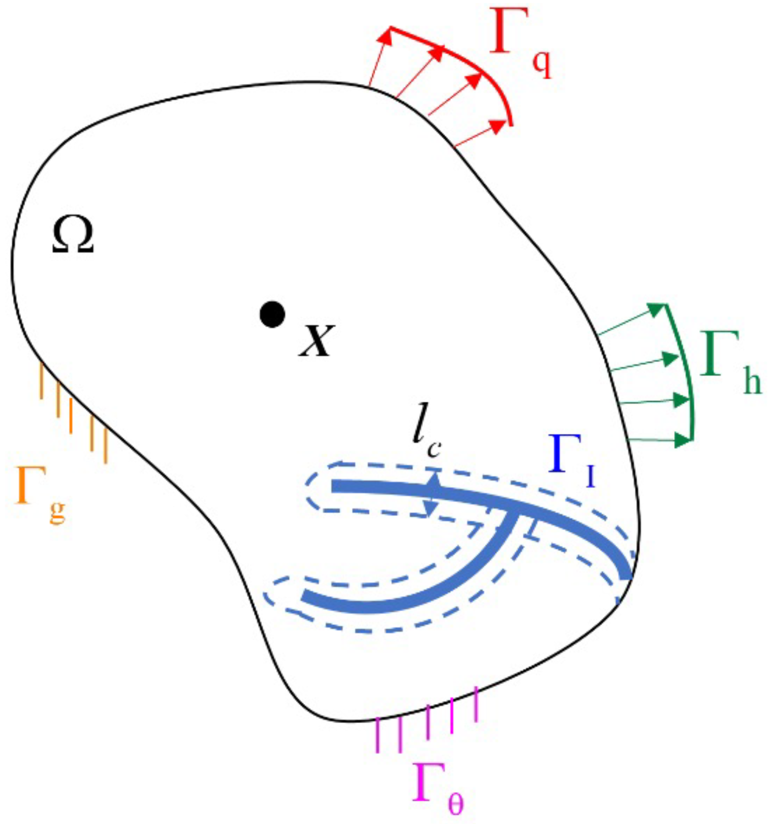
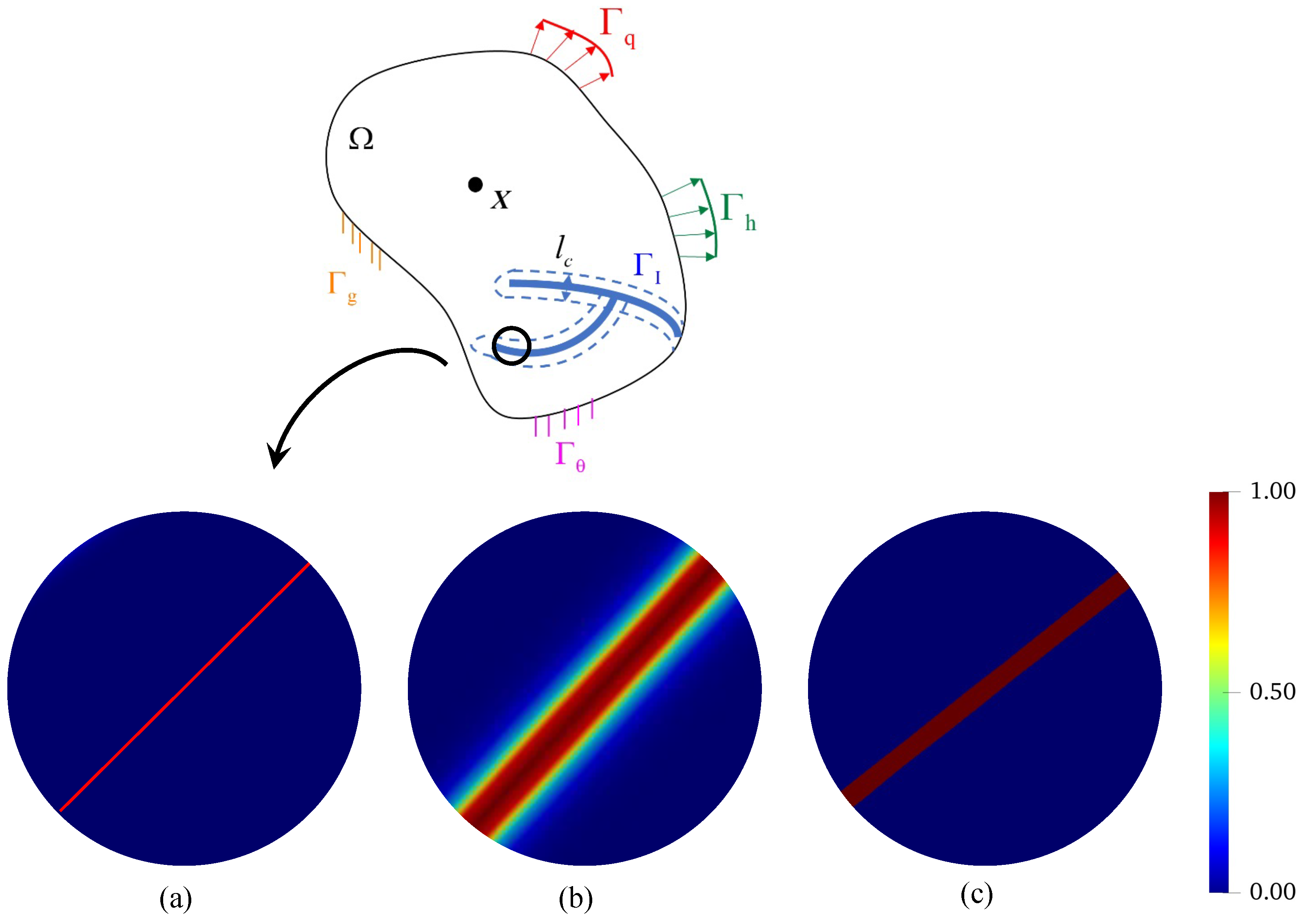
3. Governing Equations and Corresponding Weak Forms

The balance of the linear momentum, as well as the balance of the energy of the problem, are provided below:

$$\mathbf{0}=\nabla ·\mathbf{\sigma }+\rho \mathit{b}$$

(12)

$$\rho c_p\dot{\theta }=-\nabla ·\mathit{q}-T_{\mathrm{ref}}\mathit{m}:\nabla \mathit{v}+r$$

(13)

where $\mathbf{\sigma }$ is the Cauchy stress tensor, $\nabla ·(·)=\mathrm{tr}\left[\mathrm{grad}\right(·\left)\right]$ is the divergence operator, $\rho >0$ is the density, $\mathit{b}$ is the mass-specific body force, $c_p$ is the specific heat capacity, $\theta =T-T_{\mathrm{ref}}$ is the temperature difference of the current temperature T with respect to the reference temperature $T_{\mathrm{ref}}$, $\dot{\theta }$ is the time derivative of the temperature field, $\mathit{q}$ is the heat flux vector, $\mathit{v}$ is the velocity of the mechanical field, r is the heat source, and $\mathit{m}=3\kappa \beta \mathrm{I}$ is the second-order thermomechanical coupling tensor, where $\kappa$ is the bulk modulus and $\beta$ is the coefficient of thermal expansion. Using Fourier’s relation, the heat flux vector is defined as $\mathit{q}=-\mathit{k}\nabla \theta$; by assuming isotropic, $\mathit{k}=k\mathrm{I}$ is defined as the thermal conductivity.

Remark 1. 

It should be noted that Equations (12) and (13) are fully coupled through the existence of the second-order thermomechanical coupling tensor $\mathit{m}$.

The boundary conditions of this coupled problem are provided by

$$\mathit{u}=\overline{\mathit{u}}\mathrm{on}{\Gamma }_{\mathrm{g}}$$

(14)

$$\mathbf{\sigma }·\mathit{n}=\overline{\mathit{t}}\mathrm{on}{\Gamma }_{\mathrm{h}}$$

(15)

$$\theta =\overline{\theta }\mathrm{on}{\Gamma }_{\theta }$$

(16)

$$\mathit{q}·\mathit{n}=-\overline{q}\mathrm{on}{\Gamma }_{\mathrm{q}}$$

(17)

where $\overline{\mathit{u}}$, $\overline{\mathit{t}}$, $\overline{\theta }$, and $\overline{q}$ are the prescribed displacement, traction, temperature, and heat flux, respectively, and $\mathit{n}$ is the unit normal vector pointing outwards at the boundaries shown in Figure 1.

The corresponding weak forms are summarized as follows by multiplying the test functions $\{\mathbf{\eta },\delta \theta ,\delta d\}$, integrating by part, and applying the divergence theorem. The formal statement of the weak forms is as follows: given $\{{\mathcal{G}}_c,\mathcal{H},l_c,\rho ,\mathit{b},r,\overline{\mathit{u}},\overline{\mathit{t}},c_p,\mathit{k},T_{\mathrm{ref}},\overline{\theta },\overline{q}\}$, find $\{\mathit{u},\theta ,d\}$ such that Equations (18)–(20) are satisfied for all $\{\mathbf{\eta },\delta \theta ,\delta d\}$.

Weak form of the phase field:

$${\int }_{\Omega }^{}\delta d·\{g^{\prime }\left(d\right)\mathcal{H}-\frac{{\mathcal{G}}_c}{l_c}d\}d\Omega -{\int }_{\Omega }^{}{\mathcal{G}}_c{l}_c(\nabla \delta d)·(\nabla d)d\Omega =0$$

(18)

Weak form of the balance of momentum:

$${\int }_{\Omega }^{}(\nabla \mathbf{\eta }:\mathbf{\sigma }-\mathbf{\eta }·\rho \mathit{b})dV-{\int }_{{\Gamma }_{\mathrm{h}}}^{}\overline{\mathit{t}}·\mathbf{\eta }d{\Gamma }_{\mathrm{h}}=0$$

(19)

Weak form of the balance of energy:

$$\begin{array}{cc}\hfill {\int }_{\Omega }^{}[-\rho c_p\dot{\theta }·\delta \theta -\nabla \delta ·(\mathit{k}\nabla \theta )]dV+{\int }_{\Omega }^{}[-T_{\mathrm{ref}}(\mathit{m}:\nabla \mathbf{\nu })·\delta \theta +r·\delta \theta ]dV& \\ \hfill +{\int }_{{\Gamma }_{\mathrm{q}}}^{}\overline{q}·\delta \theta d{\Gamma }_{\mathrm{q}}=0\end{array}$$

(20)

In the context of phase field modeling with the expression of $g\left(d\right)$ mentioned in the previous section, in Equation (19) we can express the stress tensor in the domain as a combination of the stress for the bulk and the interface [48], as follows:

$$\mathbf{\sigma }=g\left(d\right){\mathbf{\sigma }}_{\mathrm{bulk}}+[1-g\left(d\right)]{\mathbf{\sigma }}_{\mathrm{interface}}$$

(21)

where ${\mathbf{\sigma }}_{\mathrm{bulk}}$ and ${\mathbf{\sigma }}_{\mathrm{interface}}$ are the stresses in the interior and on the interface, respectively. Equation (21) is considered a generalized expression of the stress in the phase field model for the frictional contact problem [47].

The bulk Cauchy stress tensor ${\mathbf{\sigma }}_{\mathrm{bulk}}$ is represented as $\mathbf{\sigma }=\mathbb{C}:\mathbf{ϵ}-\mathit{m}\theta$, where $\mathbb{C}$ is the fourth-order tensor representing the elastic modulus of the bulk material and $\mathbf{ϵ}$ is the strain as defined in Section 2.1. The calculation of the interface stress ${\mathbf{\sigma }}_{\mathrm{interface}}$ is discussed in Section 4 under different contact conditions.

In a similar fashion, we propose a generalized expression of the thermal conductivity $\mathit{k}$ in Equation (20) for the coupled thermomechanical problem as

$$\mathit{k}=(1-A){\mathit{k}}_{\mathrm{bulk}}+A{\mathit{k}}_{\mathrm{interface}}$$

(22)

where ${\mathit{k}}_{\mathrm{bulk}}=k_{\mathrm{bulk}}\mathrm{I}$ is the thermal conductivity of the interior domain, ${\mathit{k}}_{\mathrm{interface}}=k_{\mathrm{interface}}\mathrm{I}$ is the thermal conductivity of the interface domain, and A is a triggering value that distinguishes the bulk from the interface domain. We discuss how to decide this triggering parameter A and provide the expressions for the bulk and interface thermal conductivity ${\mathit{k}}_{\mathrm{bulk}}$ and ${\mathit{k}}_{\mathrm{interface}}$ in Section 4.

4. Stress Tensor and Thermal Conductivity Calculation for Different Contact Conditions

4.1. Stress Tensor $\mathbf{\sigma }$ Updates in the Phase Field Modeling

For the mechanical phase, following [47], updates to the Cauchy stress are made to incorporate the contact-dependent mechanical response of the interface based on different contact conditions.

We first summarize the stress tensor updates of ${\mathbf{\sigma }}_{\mathrm{interface}}$ in Equation (21) based on the different contact conditions. The normal strain is calculated to determine the following debonding/contact conditions:

$${\epsilon }_N=\mathit{\epsilon }:(\mathit{n}\otimes \mathit{n})\left\{\begin{array}{cc}\hfill >0:& \mathrm{non-contact}\\ \hfill \le 0:& \mathrm{in}\mathrm{contact}\end{array}\right.$$

(23)

For the non-contact condition with ${\epsilon }_N>0$, the stress free state results in the interface stress tensor ${\mathbf{\sigma }}_{\mathrm{interface}}=\mathbf{0}$, and there is an open crack between two surfaces. Therefore, the stress tensor in Equation (21) is expressed as $\mathbf{\sigma }=g\left(d\right){\mathbf{\sigma }}_{\mathrm{bulk}}$.

For the in contact condition with ${\epsilon }_N\le 0$, the yield function $f({\mathit{t}}_T,t_N)$ is introduced to distinguish the stick and slip conditions. The yield function $f({\mathit{t}}_T,t_N)$ with a frictional coefficient ${\mu }_f$ for the frictional Coulomb model is defined as

$$f({\mathit{t}}_T,t_N)=\parallel {\mathit{t}}_T\parallel +{\mu }_f{t}_N\left\{\begin{array}{cc}\hfill <0:& \mathrm{stick}\\ \hfill \ge 0:& \mathrm{slip}\end{array}\right.$$

(24)

where ${\mathit{t}}_T=(\mathrm{I}-\mathit{n}\otimes \mathit{n}){\mathbf{\sigma }}_{\mathrm{bulk}}$ and $t_N={\mathbf{\sigma }}_{\mathrm{bulk}}:(\mathit{n}\otimes \mathit{n})$.

When the interface is considered in the stick condition, there is no relative motion between the bulk and interface domains [47], and ${\mathbf{\sigma }}_{\mathrm{bulk}}={\mathbf{\sigma }}_{\mathrm{interface}}$ yields the stress tensor in Equation (21) as $\mathbf{\sigma }={\mathbf{\sigma }}_{\mathrm{bulk}}$. On the other hand, when the interface is considered in the slip condition with $f({\mathit{t}}_T,t_N)\le 0$, the interface stress tensor is calculated by decomposing into a frictional part ${\mathbf{\sigma }}_{\mathrm{friction}}$ and a no-penetration part ${\mathbf{\sigma }}_{\mathrm{no}-\mathrm{penetration}}$, as proposed by Fei and Choo [47], with the expressions as follows:

$${\mathbf{\sigma }}_{\mathrm{friction}}={\mu }_f{t}_N\mathrm{sign}\left({\mathit{t}}_T\right)(\mathit{n}\otimes \mathit{m}+\mathit{m}\otimes \mathit{n})$$

(25)

$${\mathbf{\sigma }}_{\mathrm{no}-\mathrm{penetration}}={\mathbf{\sigma }}_{\mathrm{bulk}}-\parallel {\mathit{t}}_T\parallel (\mathit{n}\otimes \mathit{m}+\mathit{m}\otimes \mathit{n})$$

(26)

When substituting Equations (25) and (26) into Equation (21), the overall stress tensor under the slip condition is obtained as

$$\mathbf{\sigma }={\mathbf{\sigma }}_{\mathrm{bulk}}+(1-g\left(d\right))({\mu }_f{t}_N\mathrm{sign}\left({\mathit{t}}_T\right)-\parallel {\mathit{t}}_T\parallel )(\mathit{n}\otimes \mathit{m}+\mathit{m}\otimes \mathit{n})$$

(27)

The procedures for updating the interface stress tensor ${\mathbf{\sigma }}_{\mathrm{interface}}$ and the overall stress tensor $\mathbf{\sigma }$ are summarized in Box 1, where ${\mathit{x}}_{\mathrm{int}}$ represents the geometry description of an integration point.

Box 1. Stress update algorithm for phase field modeling of the frictional contact problem.

Step 1: Inputs at ${\mathit{x}}_{int}$: strain $\mathit{\epsilon }$, phase field variable d, the normal unit vector $\mathit{n}$,

        and the tangential unit vector $\mathit{m}$.

Step 2: If the phase field variable $d=0$, THEN

     Bulk domain,

     Set $\mathbf{\sigma }={\mathbf{\sigma }}_{bulk}=\mathbb{C}:\mathit{\epsilon }-\mathit{m}\theta$,

     EXIT

Step 3: ELSE Interface domain. Calculate the normal strain ${\epsilon }_N=\mathit{\epsilon }:(\mathit{n}\otimes \mathit{n})$

     If ${\epsilon }_N>0$, THEN

      Non-contact condition, ${\mathbf{\sigma }}_{\mathrm{interface}}=\mathbf{0}$,

      Set $\mathbf{\sigma }=g\left(d\right){\mathbf{\sigma }}_{\mathrm{bulk}}$,

      EXIT

     ELSE $t_N\le 0$,

      Contact condition,

      Calculate frictional yield function $f=\parallel {\mathit{t}}_T\parallel +{\mu }_f{t}_N$,

      THEN go to Step 4.

Step 4: Contact condition.

   IF $f<0$ THEN

     Stick condition, ${\mathbf{\sigma }}_{\mathrm{interface}}={\mathbf{\sigma }}_{\mathrm{bulk}}$,

     Set $\mathbf{\sigma }=g\left(d\right){\mathbf{\sigma }}_{\mathrm{bulk}}+[1-g\left(d\right)]{\mathbf{\sigma }}_{\mathrm{interface}}={\mathbf{\sigma }}_{\mathrm{bulk}}$,

     EXIT

   ELSE,

     Slip condition, ${\mathbf{\sigma }}_{\mathrm{interface}}={\mathbf{\sigma }}_{\mathrm{friction}}+{\mathbf{\sigma }}_{\mathrm{no}-\mathrm{penetration}}$,

     Set $\mathbf{\sigma }={\mathbf{\sigma }}_{\mathrm{bulk}}+(1-g\left(d\right))\left({\mu }_f{t}_N\right)\mathrm{sign}\left({\mathit{t}}_T\right)-\parallel {\mathit{t}}_T\parallel (\mathit{n}\otimes \mathit{m}+\mathit{m}\otimes \mathit{n})$,

     EXIT

   END

4.2. Thermal Conductivity Tensor $\mathit{k}$ Updates in Phase Field Modeling

To the best of our knowledge, there is no specific formulation of thermal conductivity in the existing literature on the phase field method for coupled thermomechanical problems when considering frictional contact. In most existing phase field models, the thermal conductivity $\mathit{k}$ is degraded as $g\left(d\right)\mathit{k}$ when considering the damage effect. To accommodate frictional contact in the thermal field, we consider the heat transfer associated with the fracture damage as well as different types of thermal contact conditions. To this end, we present thermal conductivity $\mathit{k}$ updates based on four thermal conductance contact models.

As shown in the Figure 2, we enlarge the domain near the crack region in Figure 1, and the crack is shown in Figure 2a. Using the phase field method, the crack is modeled by the thin diffusive damage band shown in Figure 2b. As provided in Equation (22), the trigger parameter A is used to distinguish the bulk and interface domains. By setting the threshold to the damage value, the distribution of the trigger parameter A is shown in Figure 2c. The procedure for updating the thermal conductivity for different regions is explained in Box 2; the value of A is determined by comparing the phase field variable d with the threshold, then jumping into the corresponding thermal conductivity updates.

Remark 2. 

Recalling the phase field governing equation Equation (8), the analytical solution can be written as $d=e^{-\left|x\right|/l_c}$, where x is the distance from the current location to the nearest $d=1$ point. This argument is strong evidence for defining the damage threshold. From this equation, the width of the diffusive band is determined by the length parameter $l_c$. We set the threshold as $d=e^{-1}\approx 0.378$, where $x=l_c$, to divide the bulk and interface regions. When the damage value at the integration point surpasses this value, we assume that the interface area is entered.

With Box 2, different thermal situations can be monitored in the phase field method. In this section, we introduce four different thermal models and demonstrate how to define ${\mathit{k}}_{\mathrm{bulk}}$ and ${\mathit{k}}_{\mathrm{interface}}$ for the respective models.

Box 2. Thermal conductivity update algorithm for phase field modeling.

Step 1: Inputs at ${\mathit{x}}_{\mathrm{int}}$: phase field variable d,

         thermal conductivity ${\mathit{k}}_{\mathrm{bulk}}$ and ${\mathit{k}}_{\mathrm{interface}}$.

Step 2: Set $\mathit{k}=(1-A){\mathit{k}}_{\mathrm{bulk}}+A{\mathit{k}}_{\mathrm{interface}}$

Step 3: If $d>\mathrm{threshold}$, Interface domain

     $A=1$, THEN $\mathit{k}={\mathit{k}}_{\mathrm{interface}}$

    ELSE, Bulk domain

     $A=0$, THEN $\mathit{k}={\mathit{k}}_{\mathrm{bulk}}$

    END

Four Thermal Conductance Contact Models

Four different thermal conductance models are introduced in this section and implemented in the following applications. The definitions of ${\mathit{k}}_{\mathrm{bulk}}$ and ${\mathit{k}}_{\mathrm{interface}}$ in different thermal scenarios are displayed in

Table 1. Four different thermal conductance models with different settings of thermal conductivity $\mathit{k}$ and thermal expansion coefficient $\beta$.

Thermal Conductance Models	${\mathit{k}}_{\mathbf{bulk}}$	${\mathit{k}}_{\mathbf{interface}}$	Thermal Expansion Coefficient
Pressure dependent model (PDM)	${\mathit{k}}_{0}g\left(d\right)$	${\mathit{k}}_{0}g\left(d\right){\left(\frac{t_n}{H_e}\right)}^{{\epsilon }_c}$	$\beta =2.386\times {10}^{-3}{/}^{°}\mathrm{C}$
Uncoupled model (UCM)	${\mathit{k}}_{0}g\left(d\right)$	${\mathit{k}}_{0}g\left(d\right){\left(\frac{t_n}{H_e}\right)}^{{\epsilon }_c}$	$\beta =2.386\times {10}^{-24}{/}^{°}\mathrm{C}$
Fully conductive model (FCM)	${\mathit{k}}_0$	${\mathit{k}}_0$	$\beta =2.386\times {10}^{-3}{/}^{°}\mathrm{C}$
Adiabatic contact model (ACM)	${\mathit{k}}_{0}g\left(d\right)$	${10}^{-7}$	$\beta =2.386\times {10}^{-3}{/}^{°}\mathrm{C}$

. For the fully conductive model (FCM), the thermal conductivity is kept as a constant, assuming the whole model is in the undamaged region with $\mathit{k}={\mathit{k}}_0$. For the adiabatic model (ADM), a small enough value for the ${\mathit{k}}_{\mathrm{interface}}$ avoids heat interaction through the crack region. Normal contact stress is utilized for both the pressure-dependent (PDM) and uncoupled (UCM) models, meaning that the capability of heat transfer is dominated by both the mechanical loading and the damage effect. It is noted that the thermal expansion coefficient $\beta$ is set to be very small in the UCM in order to eliminate the coupling effect from the mechanical and thermal field.

Here, we use the pressure-dependent thermal contact model as an example to show how the process of thermal conductivity updating works. Instead of having a thermal contact conductance formulation at the contact surface, in the phase field formulation, for the first time, we develop a formulation for the interfacial thermal conductivity that is a function of the phase-field variable and the contact pressure, which accounts for the normal stress-related heat exchange through the spots. Inspired by the thermal conductance expression from discrete methods [52], we propose the following formulation for the pressure-dependent thermal conductivity:

$${\mathit{k}}_{\mathrm{interface}}=g\left(d\right){\left(\frac{t_{\mathrm{N},\mathrm{bulk}}}{H_e}\right)}^{{\epsilon }_c}{\mathit{k}}_{\mathrm{bulk}}$$

(28)

where $t_{\mathrm{N},\mathrm{bulk}}$ is the contact traction in the normal direction, $H_e$ is the Vickers hardness coefficient, and ${\epsilon }_c$ is the thermal constant. The updates for the thermal conductivity based on the pressure-dependent contact conditions are summarized in Box 3. The bulk and interface thermal domains are separated by the phase field variable d with the threshold setting. When $d<\mathrm{threshold}$, we consider the bulk domain with $A=0$, and employ the expression of ${\mathit{k}}_{\mathrm{bulk}}$ for the thermal conductivity. Otherwise, we consider the interface domain with $A=1$ and ${\mathit{k}}_{\mathrm{interface}}$. For the pressure-dependent model, we use the norm of the normal strain to differentiate the contact and debonding conditions. When ${\epsilon }_N\le 0$, we apply the pressure-dependent model to calculate ${\mathit{k}}_{\mathrm{interface}}$.

Box 3. Thermal conductivity update algorithm for phase field modeling of the pressuredependent contact model.

Step 1: Inputs at ${\mathit{x}}_{\mathrm{int}}$: the strain $\mathit{\epsilon }$, the thermal conductivity ${\mathit{k}}_0$, the phase field

         variable d, the normal unit vector $\mathit{n}$, and the tangential

         unit vector $\mathit{m}$, the threshold value: $e^{-1}\approx 0.378$.

Step 2: Set $\mathit{k}=(1-A){\mathit{k}}_{\mathrm{bulk}}+A{\mathit{k}}_{\mathrm{interface}}$

Step 3: If the phase field variable $d<\mathrm{threshold}$, Bulk domain

    $A=0$, THEN $\mathit{k}={\mathit{k}}_{\mathrm{bulk}}$

    Set ${\mathit{k}}_{\mathrm{bulk}}=g\left(d\right){\mathit{k}}_0$

    EXIT

Step 4: ELSE, the phase field variable $d\ge \mathrm{threshold}$, Interface domain

    $A=1$, THEN $\mathit{k}={\mathit{k}}_{\mathrm{interface}}$

    Calculate the normal strain ${\epsilon }_N=\mathit{\epsilon }:(\mathit{n}\otimes \mathit{n})$

    If ${\epsilon }_N>0$, THEN

      Non-contact condition,

      ${\mathit{k}}_{\mathrm{interface}}=g\left(d\right){\mathit{k}}_0$,

      EXIT

    ELSE,

      Contact condition,

      ${\mathit{k}}_{\mathrm{interface}}=g\left(d\right){\left(\frac{t_{\mathrm{N},\mathrm{bulk}}}{H_e}\right)}^{{\epsilon }_c}{\mathit{k}}_0$

    EXIT

    END

5. Numerical Examples

In this numerical simulation section, we investigate the performance of the proposed method by means of representative numerical examples. Here, we aim to: (1) demonstrate our novel thermal formulation for the thermomechanical contact problem within the context of the phase field framework; (2) verify the proposed thermomechanical phase field formulation for frictional contact problems where the fracture surfaces are stationary; and (3) validate the efficiency of the proposed method for possible crack propagation under frictional contact modeling. The coupling effect between thermal and mechanical fields is considered under different thermal contact conductance conditions. Throughout this section, all simulations are exploited in two dimensions (2D) with linear quadrilateral elements (Q4). No heat sources or body forces are introduced, and plane strain conditions are employed for all examples. For time integration, the implicit backward Euler scheme is used for the transient heat transfer and the quasi-static assumption is applied for the mechanical equilibrium equation. While the whole framework works for the transient temperature problems, all numerical examples in this section are simulated at a steady state with a large enough $\Delta t$ value to clearly observe the temperature distribution contours under different thermal scenarios.

In the following sections, we demonstrate the feasibility of the thermal formulation through two pure heat conduction problems, then compare our results with the numerical solutions from the X-FEM method in Section 5.1. Two different boundary conditions are explored, namely, the isothermal and the adiabatic situations. Then, the fully coupled thermomechanical frictional contact model is investigated, with an inner crack in Section 5.2 and a prescribed interface in Section 5.3 used to illustrate the accuracy of the proposed method. Comparisons with the literature for the mechanical phase (Section 5.2) and the coupled thermomechanical phase (Section 5.3) are presented under four different thermal contact conductance conditions. Lastly, we study a frictional crack propagation problem in Section 5.4 to show the ability of the proposed method to capture cracking phenomena using the thermomechanical coupled setting.

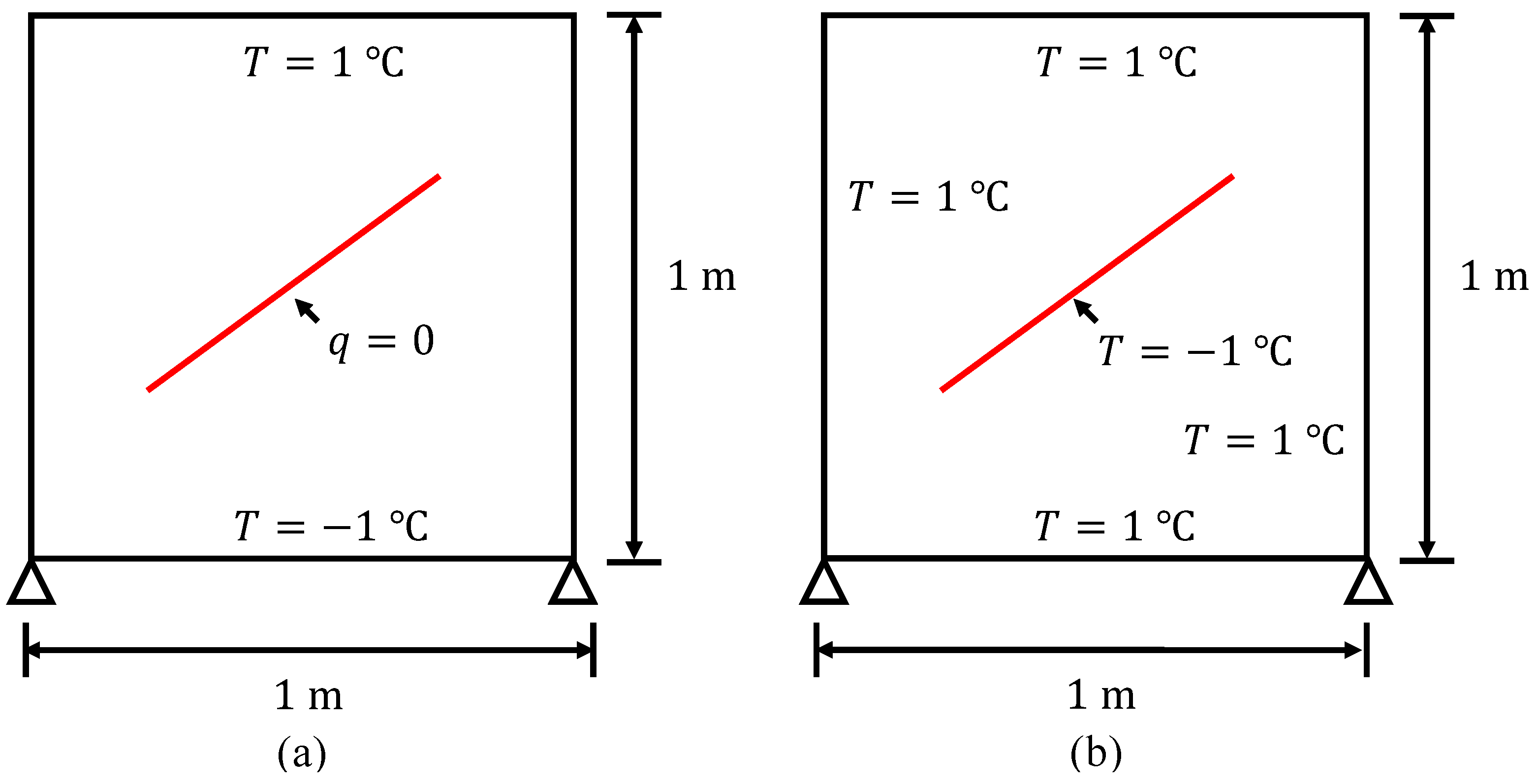
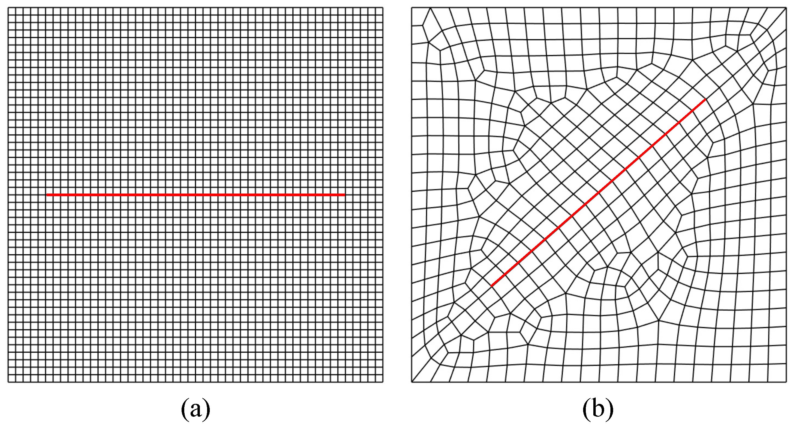
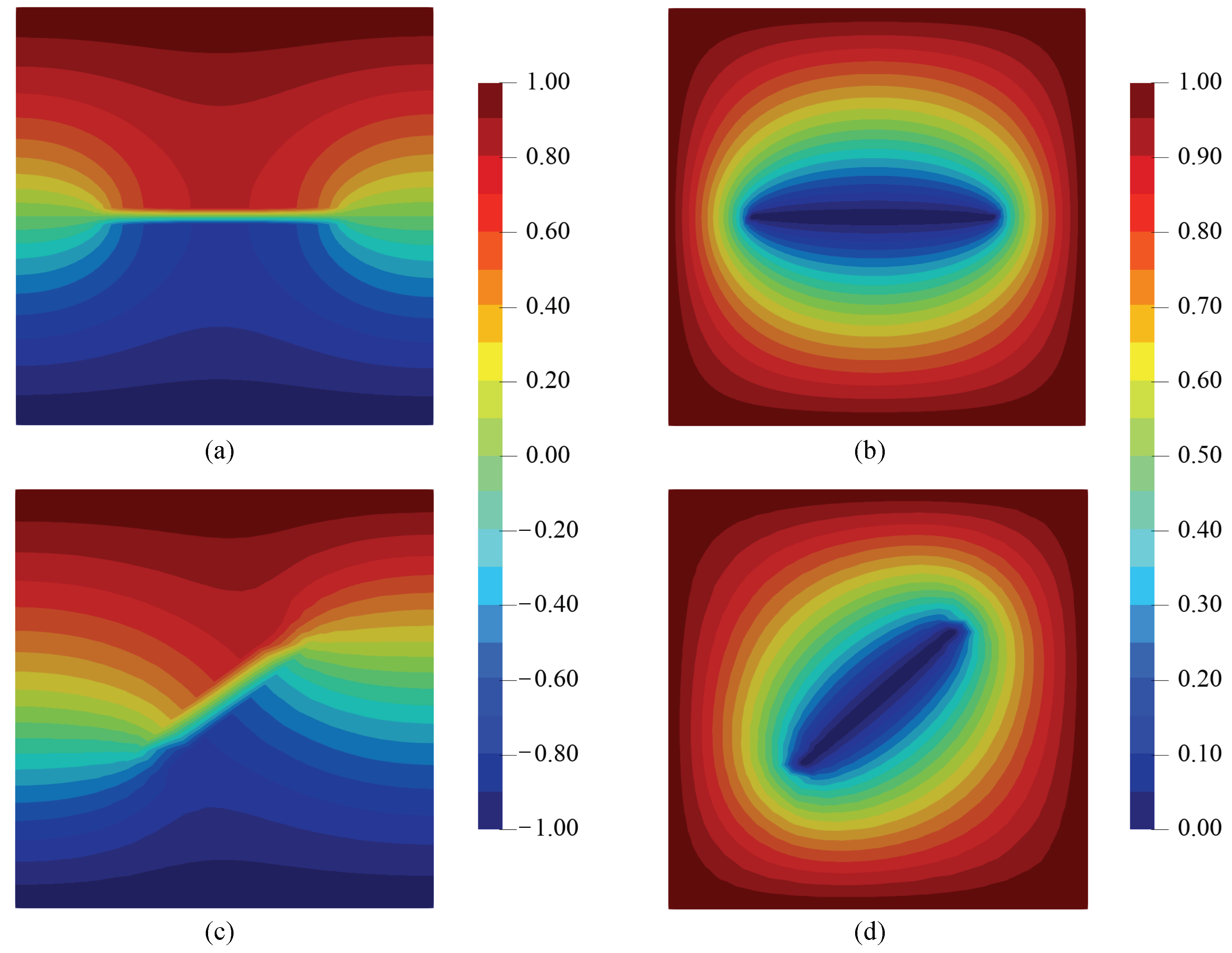
5.1. Square Plate with (a) Central Horizontal and (b) Inclined Cracks

In the first numerical example, we demonstrate the feasibility of the proposed thermomechanical coupled phase field formulation in a pure thermal setting. Two different inner cracks are utilized, namely, a horizontal crack and a slanting crack. As shown in Figure 3a,b, we first consider a square domain with a horizontal center crack that is subjected to two different thermal boundary conditions [53] for the adiabatic (Figure 3a) and isothermal (Figure 3b) cases. For the adiabatic case, temperatures of $T=1{}^{°}\mathrm{C}$ and $T=-1{}^{°}\mathrm{C}$ are imposed on the top and bottom surfaces, respectively, with no heat flux transferring across the crack [49]. For the isothermal case, the temperature is maintained at $T=1{}^{°}\mathrm{C}$ for all edge surfaces, while the temperature field of the inner crack is different from the boundaries, with $T=-1{}^{°}\mathrm{C}$. Figure 4 depicts the results for the model with a slant center crack using the same thermal boundary settings.

For the horizontal center crack model shown in Figure 3, the block size is $2\mathrm{m}\times 2\mathrm{m}$, with the red line depicting the inner crack. The inner crack is located in the middle, with crack length a of $1.2\mathrm{m}$, meaning that $a/L=0.6$, where L is the side length of the domain. The mesh size of this simulation is $50\times 50$, as shown in Figure 5a, with the length parameter set to $l_c=0.16\mathrm{m}$. For the adiabatic case, in order to guarantee that the heat transferring through the crack is small enough to be ignored, the interface thermal conductance ${\mathit{k}}_{\mathrm{interface}}$ is set to ${10}^{-7}\mathrm{W}/\mathrm{mm}{}^{°}\mathrm{C}$.

For the slant center crack, as illustrated in Figure 4, the domain size is $1\mathrm{m}\times 1\mathrm{m}$, with a stationary crack starting from $(0.3\mathrm{m},0.33\mathrm{m})$ to $(0.7\mathrm{m},0.68\mathrm{m})$. The problem domain is discretized by unstructured meshes, as shown in Figure 5b, with an approximated mesh size of $h=0.05\mathrm{m}$ and with $l_c=0.2\mathrm{m}$. Detailed material properties for these two crack models are summarized in

Table 2. Detailed material properties for the square plate with cracks.

Bulk Material
Young’s modulus	E	10,000 MPa
Poisson’s ratio	$\nu$	0.3
Density	$\rho$	$2.7\times {10}^{-9}{\mathrm{kg}/\mathrm{mm}}^3$
Thermal expansion coefficient	$\beta$	$2.386\times {10}^{-24}{/}^{°}\mathrm{C}$
Bulk thermal conductivity	${\mathit{k}}_{\mathrm{bulk}}$	$150{\mathrm{W}/\mathrm{mm}}^{°}\mathrm{C}$
Interface thermal conductivity (for adiabatic case)	${\mathit{k}}_{\mathrm{interface}}$	${10}^{-7}{\mathrm{W}/\mathrm{mm}}^{°}\mathrm{C}$

.

The resulting contour plots of the temperature distribution for the models with horizontal and slant center cracks under two different thermal conditions (the adiabatic and isothermal cases) are exhibited in Figure 6. For the adiabatic case, shown in Figure 6a,c, the discontinuities in the thermal field are clearly shown near the fracture region, as the two sides of the crack are supposed to be insulated from each other. The width of the observed crack is controlled by the length parameter $l_c$, which is the width of the diffusive damage band. On the other hand, for the isothermal case, shown in Figure 6b,d, the thermal contours are uniformly distributed. Compared to the analysis in [49,53], where the X-FEM method is used, we observe that the results match remarkably well with the reference. This agreement demonstrates that the proposed thermomechanical coupled phase field formulation is able to correctly identify and reproduce the temperature discontinuity and continuity profile near the crack regions for both the isothermal and adiabatic cases.

Remark 3. 

For the adiabatic case, as shown in Table 2, ${\mathit{k}}_{\mathrm{interface}}$ should be set with a sufficiently small value rather than 0 in order to avoid any singularity in the matrix calculation.

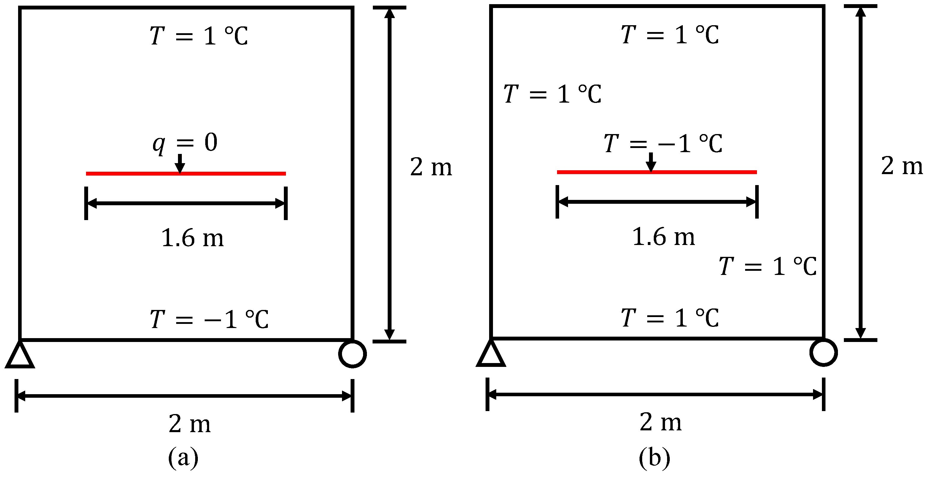
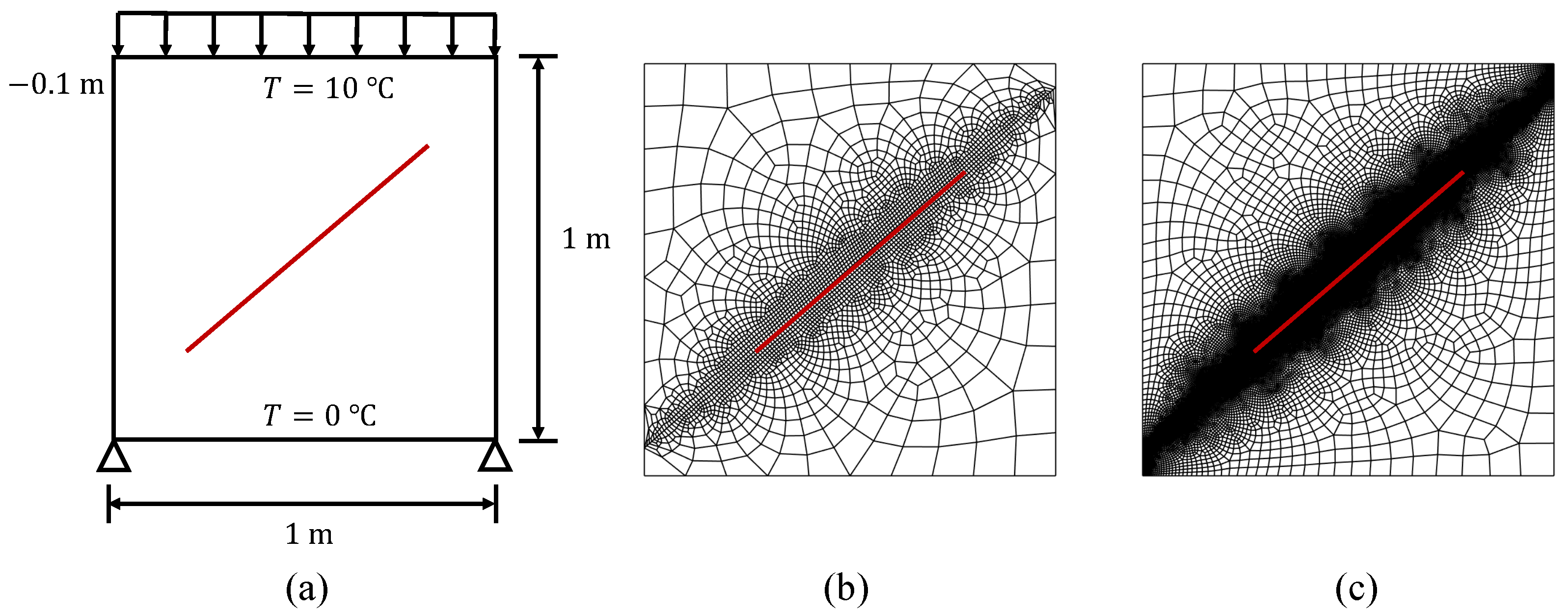
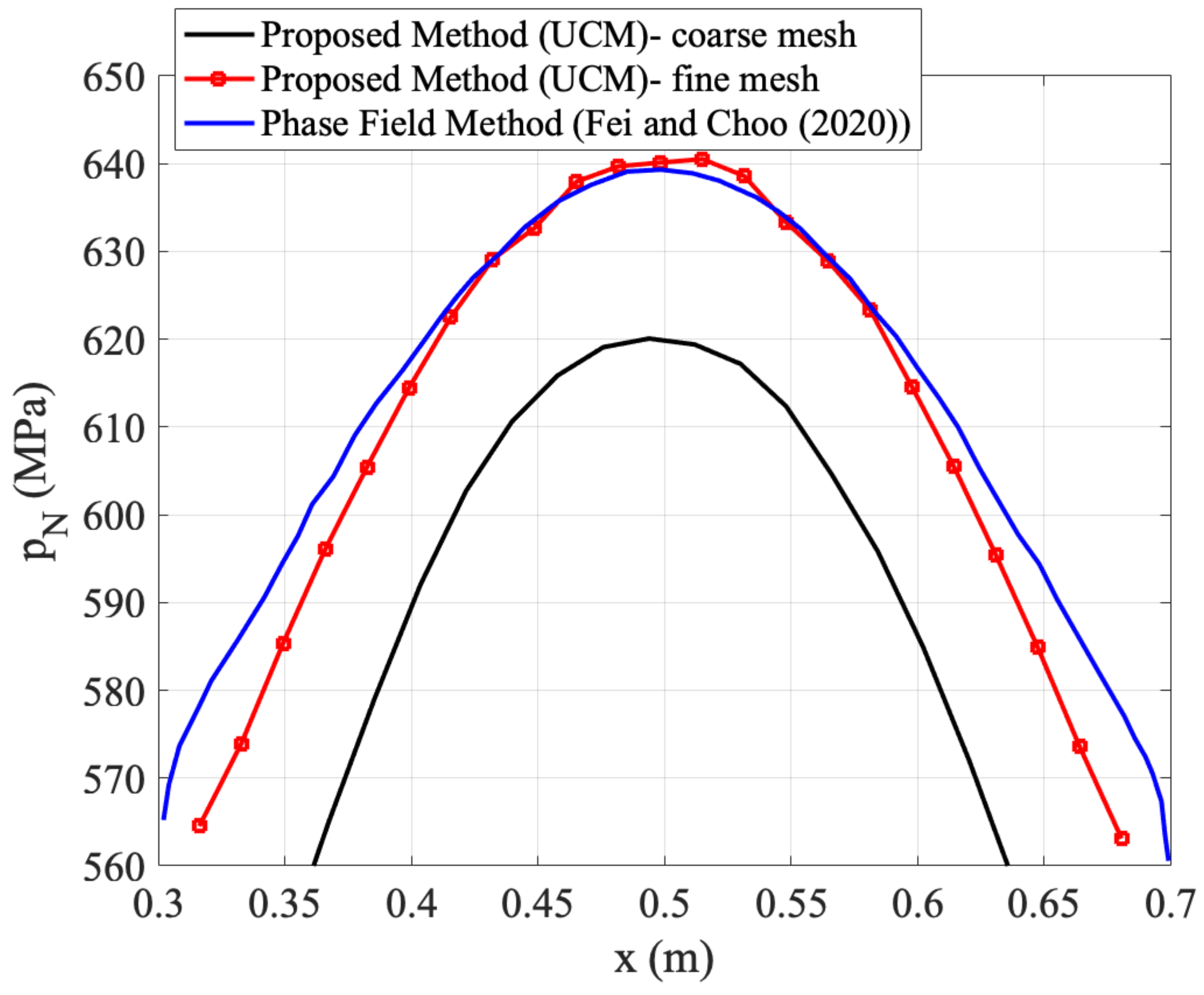
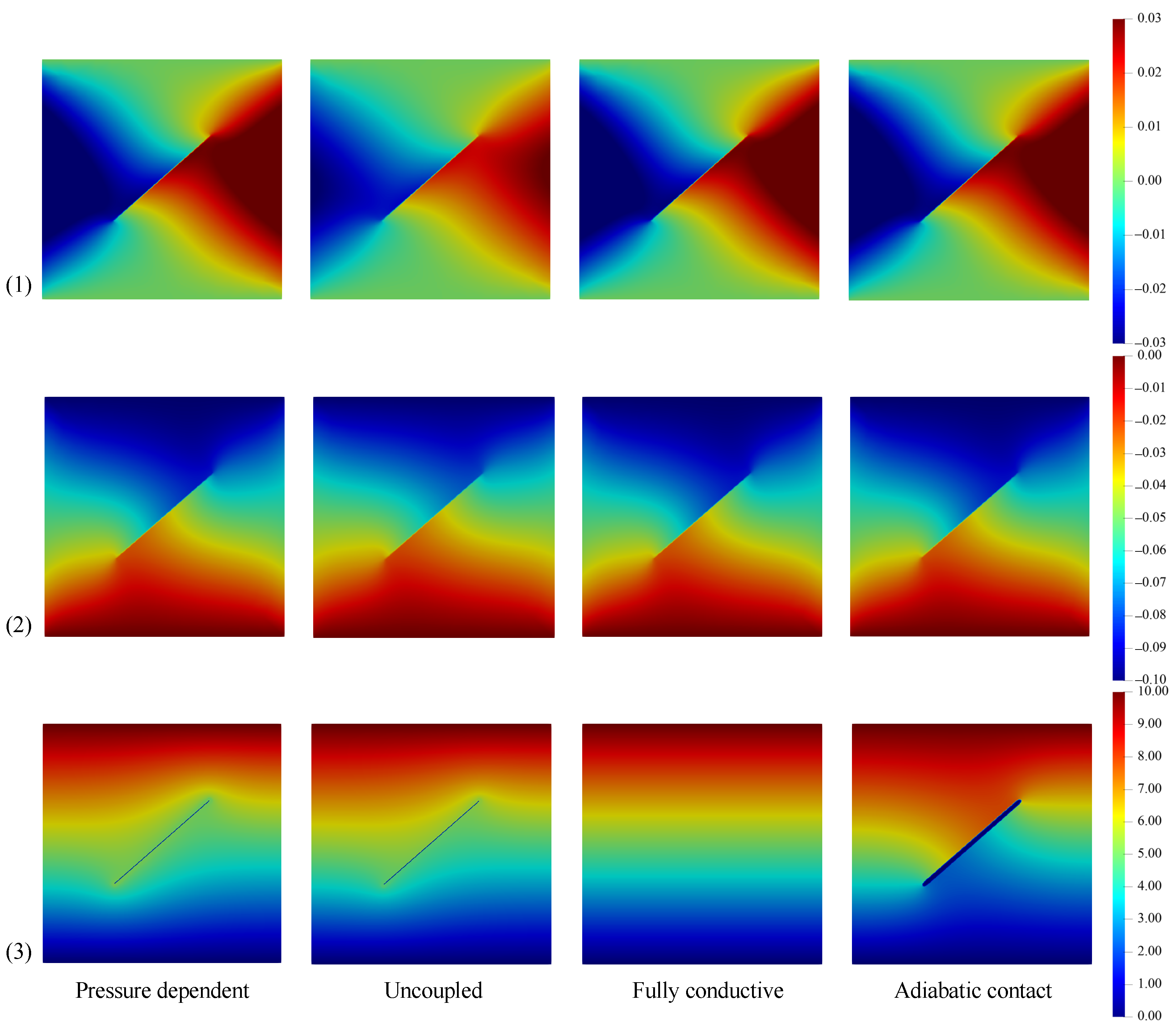
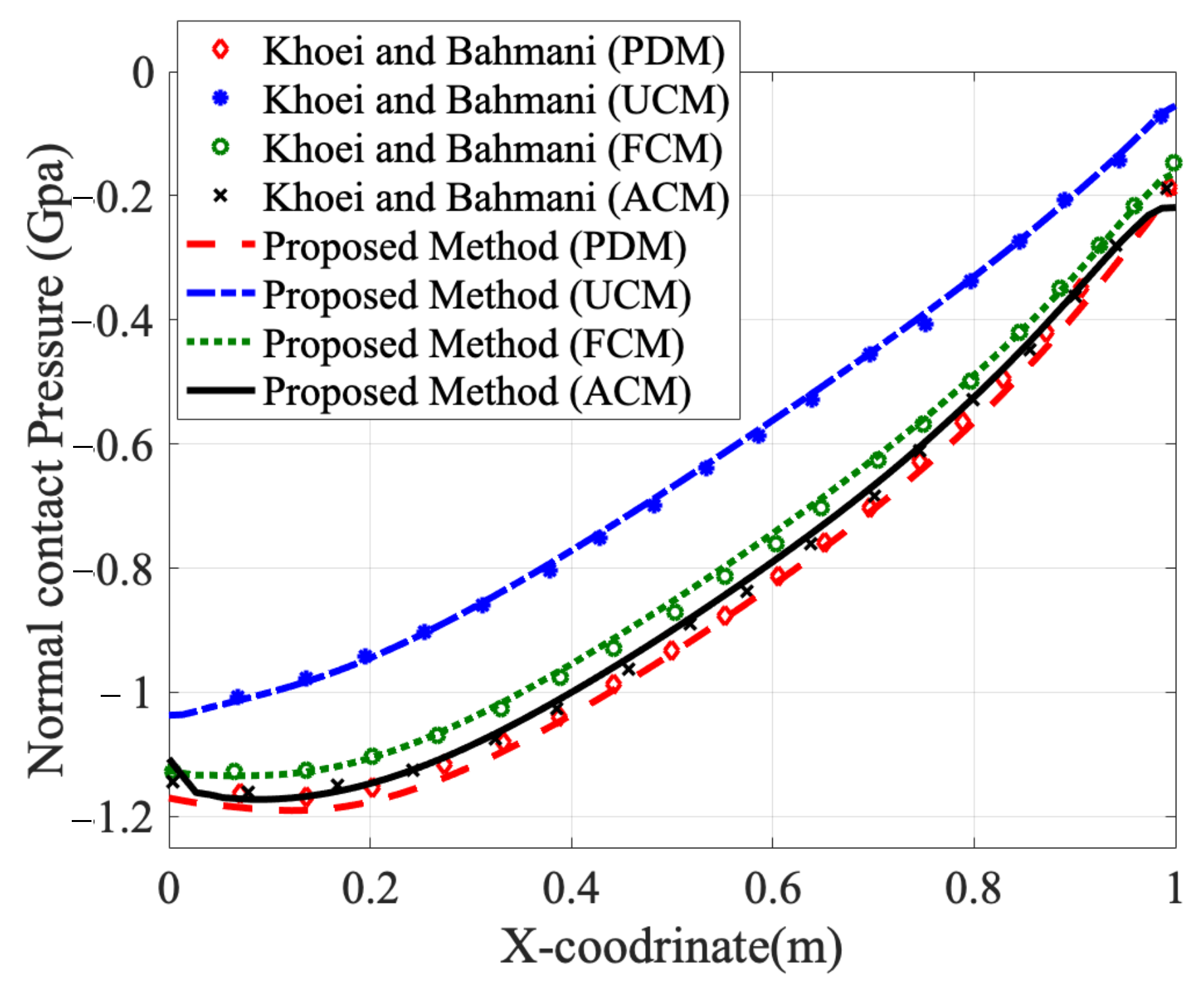
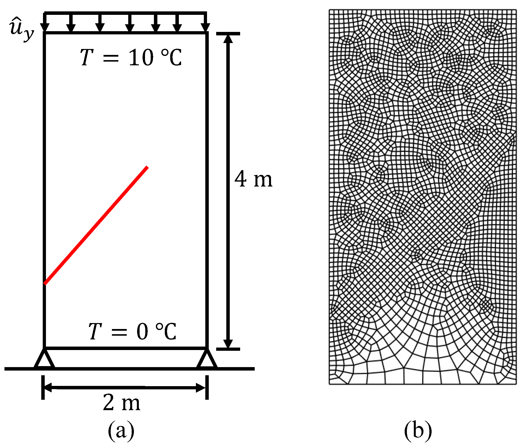
5.2. Squared Domain with an Internal Slant Frictional Crack

After validating the pure thermal problem, we extend the model with the slant center crack in Section 5.1 to model a thermomechanical coupled problem with a frictional contact crack. The purpose of the second example is to investigate the ability of the proposed phase field method for thermomechanical problems with frictional contact. The problem was initially proposed by Dolbow et al. [20], and was later elaborated in [48] to verify the phase field method for frictional contact cracks in purely mechanical problems. As shown in Figure 7a, the geometry of the domain is a $1\mathrm{m}\times 1\mathrm{m}$ square with an existing crack located from $(0.3\mathrm{m},0.33\mathrm{m})$ to $(0.7\mathrm{m},0.68\mathrm{m})$ [48]. A uniform displacement loading $d=-0.1\mathrm{m}$ in total is applied on the top surface in 10 steps. We adopt the same material properties used in [48], with elastic modulus $E=10,000\mathrm{MPa}$, Poisson’s ratio $\nu =0.3$, and the frictional coefficient of the crack surface ${\mu }_f=0.1$. The two fractional mesh distributions are shown in Figure 7, in (b) with coarse mesh size $h=0.008\mathrm{m}$, $l_c=0.032\mathrm{m}$ and in (c) with the finest mesh size $h=0.002\mathrm{m}$, $l_c=0.008\mathrm{m}$ are investigated in this section. In this simulation, the crack driving force parameter $\mathcal{H}$ is calculated following the same strategy as in Appendix A of Borden et al. [4], and the critical fracture energy is set to ${\mathcal{G}}_c=50{\mathrm{N}/\mathrm{m}}^2$.

As the main focus of this paper, we investigate the effect of the different thermal conductance conditions on the mechanical phase. In addition to mechanical loading, we apply the thermal boundary conditions shown in Figure 7a, with $10{}^{°}\mathrm{C}$ prescribed to the top surface and $0{}^{°}\mathrm{C}$ to the bottom surface, for further exploration.

In Table 1, we display different thermal conductance models with different thermal conductivity $\mathit{k}$ as provided in Equation (22). The thermal expansion coefficients are presented in Table 1. The four different thermal conductivity models discussed in Section 4.2, namely, the pressure-dependent model (PDM), uncoupled model (UCM), fully conductive model (FCM), and adiabatic contact model (ACM), are employed. First, we compare the normal contact stress along the crack with [47] using the uncoupled model (Figure 8). The comparison shows that with mesh refinement, the proposed method approaches the reference solution with good agreement.

The results of the displacement and temperature contours at the last step using the fine mesh are shown in Figure 9. It can be noted that for the uncoupled case (UCM), we set the thermal expansion coefficient to be small enough that the coupling effect can be ignored. Comparing our results with the purely mechanical simulation presented in Fei and Choo’s work [48], excellent agreement on the displacement contours is achieved. For the other three cases with thermal effects, displacements in the x direction are more significant compared to the UCM case due to coupled thermomechanical effects. Because the displacement in the y direction is fixed, there is not much difference shown on contour plots in Figure 9.

As for the thermal field, the temperature distribution is uniform in the fully conductive model with the same thermal conductivity for the bulk (${\mathit{k}}_{\mathrm{bulk}}$) and the interface (${\mathit{k}}_{\mathrm{interface}}$) domains. Thus, in the fully conductive case shown in Figure 9 (3), the location of the inclined crack is not visible. For the other three models, the fracture crack in the temperature contours can be clearly observed. As shown in Table 1, sharing the same ${\mathit{k}}_{\mathrm{interface}}$, which is determined by the contact pressure and damage parameter, the difference in the temperature distribution for the PDM and UCM case is dominated by the coupling term between the thermal and mechanical field. As shown in Figure 9 (3), the PDM case with a stronger coupling effect exhibits a more continuous temperature distribution around the crack region. In the adiabatic model (ACM), with ${\mathit{k}}_{\mathrm{interface}}$ set to be a small enough constant, there is almost no heat transference in that area, and strong discontinuity in the temperature field is visible.

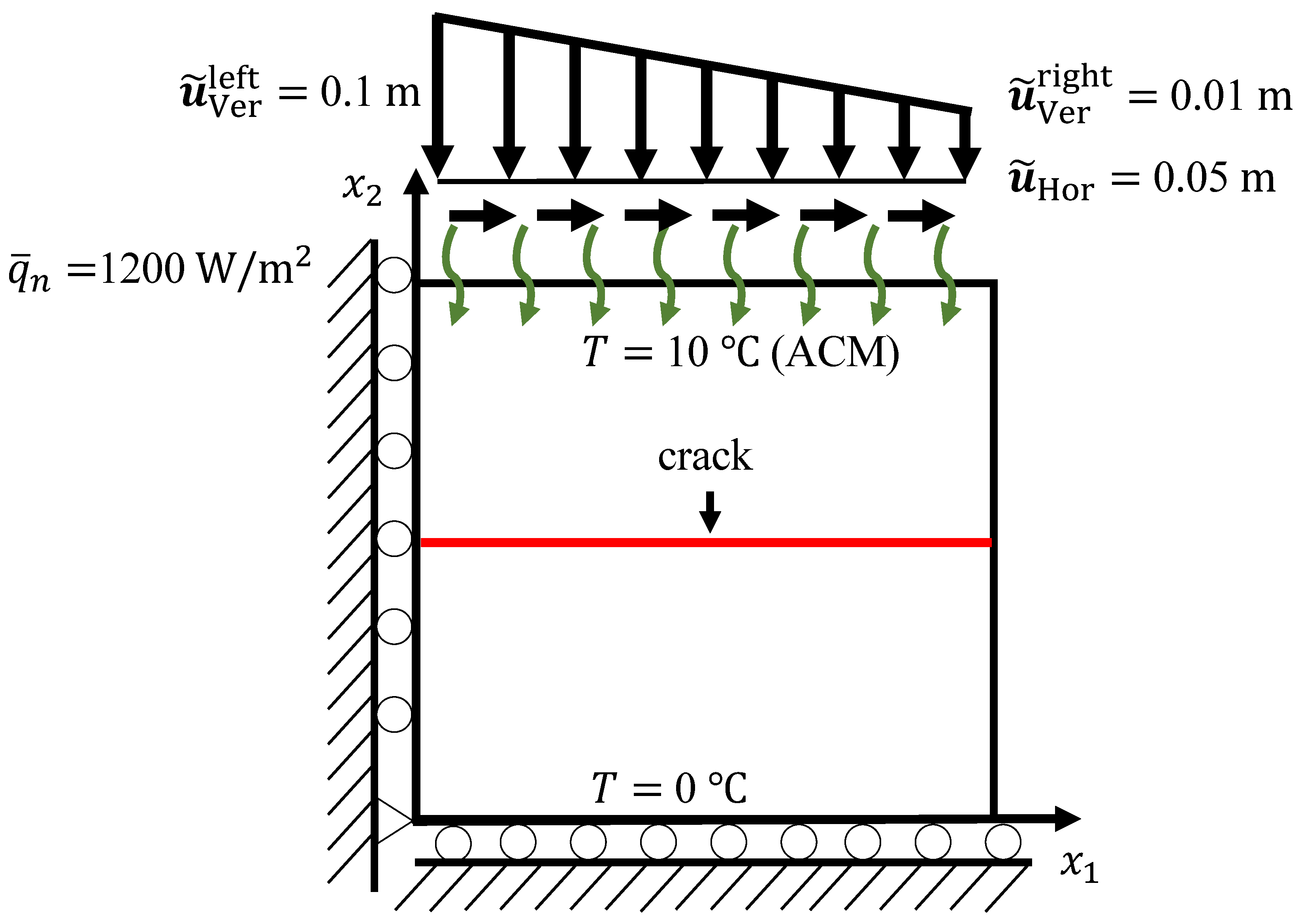
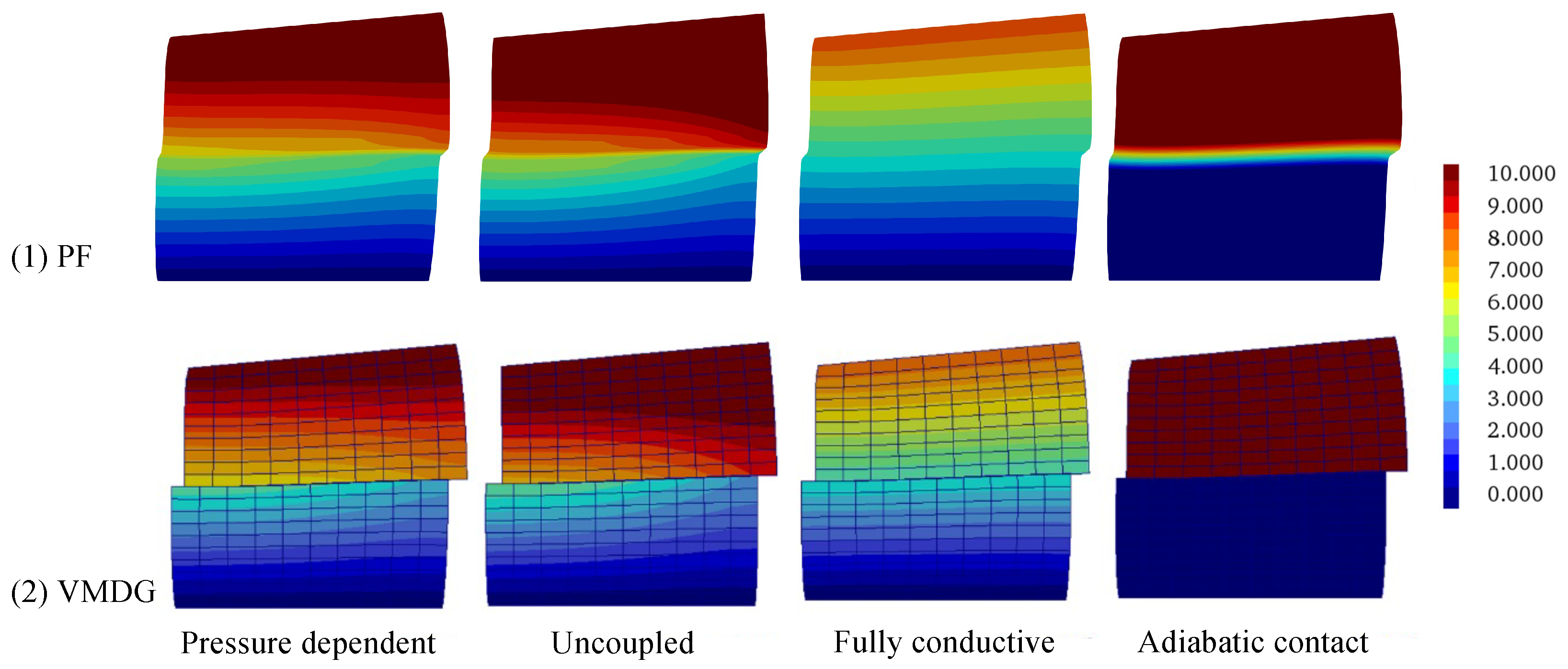
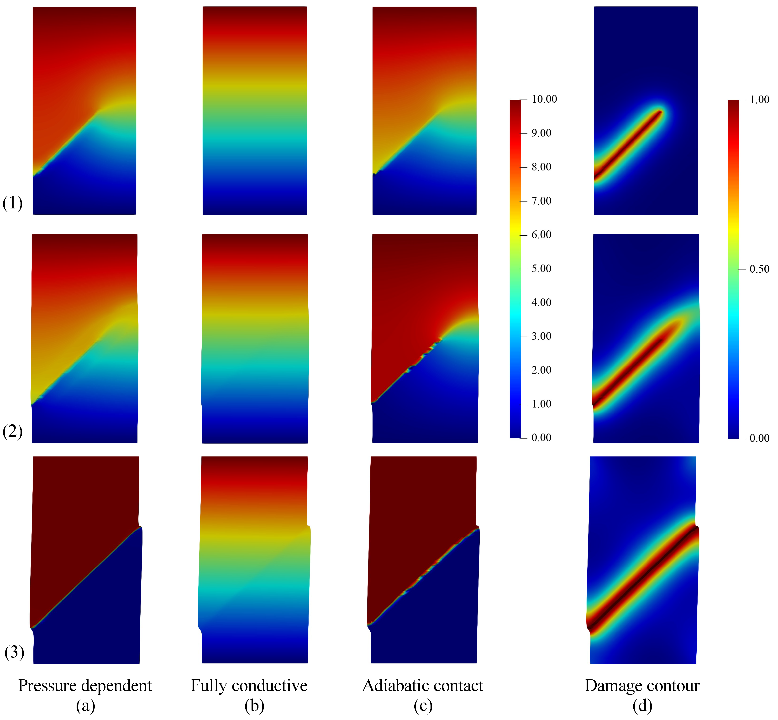
5.3. The Frictional Sliding Problem under Different Thermomechanical Coupled Conditions

In this section, we use the proposed frictional contact model to solve a frictional sliding problem. The problem was simulated in our previous paper, where a discrete VMDG method was used [50]. The detailed geometry is shown in Figure 10, where the $1\mathrm{m}\times 1\mathrm{m}$ domain is subjected to two prescribed displacement loadings on the top surface. In addition, a heat flux ${\overline{q}}_n=1200{\mathrm{W}/\mathrm{m}}^2$ is applied on the top surface pointing inward, with $0{}^{°}\mathrm{C}$ fixed on the bottom surface. The total displacement is applied in 10 steps, while the time increment $\Delta t$ is set to be $\Delta t=2.8\times {10}^{16}\mathrm{s}$ to ensure that the thermal phase is in the quasi-static state. As stated in Section 4.2, four different thermal conductivity conditions are considered, as provided in Table 1. For the adiabatic contact model (ACM), as mentioned in [52], it should be noted that the heat flux boundary condition must be replaced by the temperature boundary condition $T=10{}^{°}\mathrm{C}$ on the top surface to avoid the singularity in the equations of the thermal system. The detailed material properties are provided in

Table 3. Detailed material properties of the frictional sliding problem.

Poisson’s ratio	$\nu =0.3$
Young’s modulus	$E=1.0\times {10}^4\mathrm{MPa}$
Thermal conductivity	$k=150\mathrm{W}/\mathrm{m}{}^{°}\mathrm{C}$
Thermal conductance coefficient	$h_{c0}=6.5\times {10}^{-5}\mathrm{W}/\mathrm{m}{}^{°}\mathrm{C}$
Vickers hardness	$H_e=100\mathrm{MPa}$
Thermal constant	${\epsilon }_c=1$
Frictional coefficient	$\mu =0.1$

.

In Figure 11, the contours of temperature distribution are shown in their deformed configurations. A comparison is performed in this figure among the different thermal contact conductivity models, i.e., PDM, UCM, FCM, and ADM. In addition, we compare the results with our previous work [50], where the VMDG method was used. Very good agreement is achieved between the proposed phase field method and the previous VMDG method. It is noted that a slight difference in the temperature contour between the VMDG and the proposed phase field method can be observed in the adiabatic case, as shown in Figure 11. Because the discontinuity is controlled by the length parameter $l_c$ in the phase field method, when s smaller length parameter is applied the sharper discontinuity is captured in the temperature as well as the displacement. The VMDG method is a discrete method with duplicated nodes at the fracture surface; thus, the sharp discontinuity in the displacement is captured exactly. In contrast, in the proposed phase field method, discontinuity is captured in a diffuse fashion influenced by the mesh size and the length parameter $l_c$.

To further assess the performance and accuracy of the proposed phase field model for the frictional sliding problem, we compare the normal contact stress results with Khoei and Bahmani’s [52] analysis, where the X-FEM method was used. As in [52], we use a uniform structured FE mesh of $75\times 75$ quadrilateral elements, and the penalty parameters are used to constrain the tangential and normal stick conditions. As shown in Figure 12, a strong agreement is achieved when comparing the proposed phase field method to the X-FEM method. As stated in the previous sections, the proposed phase field method does not require a specific treatment or algorithm at the contact surface and is easier to implement compared to discrete methods.

5.4. Propagation of an Inclined Crack in a Rectangular Plate

To enrich the applications of the proposed method, in this example we simulate the crack propagation to demonstrate the capacity of the framework following the verification of the stationary interface problems. As shown in Figure 13a, a rectangular domain with geometry $2\mathrm{m}\times 4\mathrm{m}$ has a ${45}^{°}$ inclined crack located between $(0.0\mathrm{m},0.7\mathrm{m})$ and $(1.3\mathrm{m},2.0\mathrm{m})$. Proportional displacement loading ${\widehat{u}}_y=-2\times {10}^{-4}\mathrm{m}$ is prescribed on the top surface in 100 load steps. For the thermal phase, the temperature on the top surface is set to $10{}^{°}\mathrm{C}$ while it is $0{}^{°}\mathrm{C}$ for the bottom surface. The material parameters used in this example are $E=10,000\mathrm{MPa}$, $\nu =0.3$, ${\mu }_f=0.01$, and ${\mathcal{G}}_c=50{\mathrm{kJ}/\mathrm{m}}^2$. The mesh size of this problem is approximately $0.05\mathrm{m}$. as shown in Figure 13b, with the length parameter set to $l_c=0.2\mathrm{m}$.

Following the algorithm proposed by Amor [54], the strain history energy $\mathcal{H}$ should be updated and employed in the calculation at each load step, rather than arbitrarily defined as for stationary cracks, owing to the dynamic crack propagation. This means that the evolution of the phase field damage parameter d is dependent on the displacement from previous steps. The thermal expansion coefficient $\beta$ is chosen to be a relatively small number in this simulation.

The evolution of the phase field parameter d and the temperature contour plots are shown in Figure 14 at three different load steps and with three different thermal contact conductance models. The propagation of the crack and the evolution of the temperature are clearly captured using the proposed phase field method. For the fully conductive case (FCM), the temperature is uniformly distributed, as the heat is free to transfer between the upper and lower parts of the domain. For the adiabatic case (ACM), the temperature field exhibits a sharp discontinuity across the damaged crack. As the crack propagates, the temperature distribution shows a stronger discontinuity, while the damage region expands. At the last load step, when the crack is fully developed, and the whole domain is separated into two parts, and the temperature fields of the upper and lower parts are completely discontinuous. For the pressure-dependent model (PDM), when compared to the ACM case, heat transfer is more obvious at the beginning of the crack propagation process, as it is dependent on the magnitude of the contact stress at the crack region. During the crack initiation and propagation stage, the temperature discontinuity becomes less distinguishable as the crack propagates, because ${\mathit{k}}_{\mathrm{interface}}$ is dominated by increasing displacement loading rather than the phase field damage variable d. After the crack is fully developed, the damage variable is dominated by the conductivity, and there is no thermal interaction between the two subdomains.

6. Concluding Remarks

In this paper, a thermomechanical coupled phase field method has been developed for modeling cracks with frictional contact. In the mechanical phase, the proposed method follows the work of Fei and Choo [48], regularizing the stress tensor at contact regions under different contact conditions, with a specific focus on frictional contact to accommodate the no-penetration constraints. For the thermal phase, we propose a novel formulation for thermal conductivity in a regularized contact region by accommodating different thermal conductance conditions and the phase field damage parameter. We investigate several benchmark examples to assess the proposed computational method. First, we verify the proposed thermal algorithm using different pure thermal models. Then, we simulate a problem with an internal slant frictional crack and extend the model into thermomechanical coupled fields. In the third example, we study the thermomechanical coupled frictional sliding problem and compare the results with the X-FEM and the VMDG methods, finding good agreement, which demonstrates the capacity of the proposed phase field framework in simulating coupled thermomechanical problems with frictional sliding. Lastly, we demonstrate that the proposed method can simulate crack propagation with thermal effects. Based on the above conclusions, the proposed method has potential applications in various areas, including modeling of thermomechanical coupled crack propagation of composite structures, deposition processes in friction stir welding, and metal forming processes.

There are several key features in this paper, including (i) the formulation accommodates no-penetration constraints of the contact behavior in the phase field method and (ii) the formulation accommodates different thermal conductance conditions without the need for a sophisticated algorithm to impose thermal contact constraints on crack surfaces. The proposed phase field method can be implemented easily in comparison to the existing discrete methods for frictional cracks. The proposed model can be applied in the future for complex geometry and crack branching, and merging in coupled multi-physics settings. Although the proposed thermomechanical coupled phase field method is promising, it has a number of deficiencies. The main limitations are threefold. First, the inertial effect in the mechanical field is not considered. Second, in terms of accuracy, the phase field method does not show superior performance for stationary cracks compared to discrete methods. Third, without duplicating nodes at the cracking interfaces it is difficult to capture the sharp discontinuity along the cracking surfaces. With all these considerations, our future work will focus on advancing the model in order to (1) accommodate dynamic effects in the mechanical field, (2) adopt a discrete method for predefined crack regions to capture the sharp discontinuities, and (3) track both stationary interface cracks and propagating cracks simultaneously. Work is underway to adopt the VMDG method [50] to model stationary interfaces and combine it with the present phase field model for crack propagation.

References

1. Chaboche, J.L. Development of continuum damage mechanics for elastic solids sustaining anisotropic and unilateral damage. Int. J. Damage Mech. 1993, 2, 311–329. [Google Scholar] [CrossRef]
2. Seitz, A.; Wall, W.A.; Popp, A. Nitsche’s method for finite deformation thermomechanical contact problems. Comput. Mech. 2019, 63, 1091–1110. [Google Scholar] [CrossRef]
3. Miehe, C.; Hofacker, M.; Welschinger, F. A phase field model for rate-independent crack propagation: Robust algorithmic implementation based on operator splits. Comput. Methods Appl. Mech. Eng. 2010, 199, 2765–2778. [Google Scholar] [CrossRef]
4. Borden, M.J.; Verhoosel, C.V.; Scott, M.A.; Hughes, T.J.; Landis, C.M. A phase-field description of dynamic brittle fracture. Comput. Methods Appl. Mech. Eng. 2012, 217, 77–95. [Google Scholar] [CrossRef]
5. Hansbo, P.; Lovadina, C.; Perugia, I.; Sangalli, G. A Lagrange multiplier method for the finite element solution of elliptic interface problems using non-matching meshes. Numer. Math. 2005, 100, 91–115. [Google Scholar] [CrossRef]
6. Hirmand, M.; Vahab, M.; Khoei, A. An augmented Lagrangian contact formulation for frictional discontinuities with the extended finite element method. Finite Elem. Anal. Des. 2015, 107, 28–43. [Google Scholar] [CrossRef]
7. Simo, J.C.; Laursen, T. An augmented Lagrangian treatment of contact problems involving friction. Comput. Struct. 1992, 42, 97–116. [Google Scholar] [CrossRef]
8. Dittmann, M.; Franke, M.; Temizer, I.; Hesch, C. Isogeometric analysis and thermomechanical mortar contact problems. Comput. Methods Appl. Mech. Eng. 2014, 274, 192–212. [Google Scholar] [CrossRef] [Green Version]
9. Cardiff, P.; Karač, A.; Ivanković, A. Development of a finite volume contact solver based on the penalty method. Comput. Mater. Sci. 2012, 64, 283–284. [Google Scholar] [CrossRef] [Green Version]
10. Chouly, F.; Fabre, M.; Hild, P.; Mlika, R.; Pousin, J.; Renard, Y. An overview of recent results on Nitsche’s method for contact problems. In Geometrically Unfitted Finite Element Methods and Applications; Springer: Berlin/Heidelberg, Germany, 2017; pp. 93–141. [Google Scholar]
11. Wriggers, P.; Zavarise, G. A formulation for frictionless contact problems using a weak form introduced by Nitsche. Comput. Mech. 2008, 41, 407–420. [Google Scholar] [CrossRef]
12. Arnold, D.N. An interior penalty finite element method with discontinuous elements. SIAM J. Numer. Anal. 1982, 19, 742–760. [Google Scholar] [CrossRef] [Green Version]
13. Nitsche, J. Über ein Variationsprinzip zur Lösung von Dirichlet-Problemen bei Verwendung von Teilräumen, die keinen Randbedingungen unterworfen sind. Abh. Math. Semin. Univ. Hambg. 1971, 36, 9–15. [Google Scholar] [CrossRef]
14. Sanders, J.D.; Laursen, T.A.; Puso, M.A. A Nitsche embedded mesh method. Comput. Mech. 2012, 49, 243–257. [Google Scholar] [CrossRef]
15. Annavarapu, C.; Hautefeuille, M.; Dolbow, J.E. A robust Nitsche’s formulation for interface problems. Comput. Methods Appl. Mech. Eng. 2012, 225, 44–54. [Google Scholar] [CrossRef]
16. Truster, T.J.; Chen, P.; Masud, A. Finite strain primal interface formulation with consistently evolving stabilization. Int. J. Numer. Methods Eng. 2015, 102, 278–315. [Google Scholar] [CrossRef]
17. Masud, A.; Chen, P. Thermoelasticity at finite strains with weak and strong discontinuities. Comput. Methods Appl. Mech. Eng. 2019, 347, 1050–1084. [Google Scholar] [CrossRef]
18. Francfort, G.A.; Marigo, J.J. Revisiting brittle fracture as an energy minimization problem. J. Mech. Phys. Solids 1998, 46, 1319–1342. [Google Scholar] [CrossRef]
19. Moës, N.; Dolbow, J.; Belytschko, T. A finite element method for crack growth without remeshing. Int. J. Numer. Methods Eng. 1999, 46, 131–150. [Google Scholar] [CrossRef]
20. Dolbow, J.; Moës, N.; Belytschko, T. An extended finite element method for modeling crack growth with frictional contact. Comput. Methods Appl. Mech. Eng. 2001, 190, 6825–6846. [Google Scholar] [CrossRef] [Green Version]
21. Fries, T.P.; Belytschko, T. The extended/generalized finite element method: An overview of the method and its applications. Int. J. Numer. Methods Eng. 2010, 84, 253–304. [Google Scholar] [CrossRef]
22. Armero, F.; Garikipati, K. An analysis of strong discontinuities in multiplicative finite strain plasticity and their relation with the numerical simulation of strain localization in solids. Int. J. Solids Struct. 1996, 33, 2863–2885. [Google Scholar] [CrossRef]
23. Oliver, J. Modelling strong discontinuities in solid mechanics via strain softening constitutive equations. Part 1: Fundamentals. Int. J. Numer. Methods Eng. 1996, 39, 3575–3600. [Google Scholar] [CrossRef]
24. Armero, F.; Linder, C. New finite elements with embedded strong discontinuities in the finite deformation range. Comput. Methods Appl. Mech. Eng. 2008, 197, 3138–3170. [Google Scholar] [CrossRef]
25. Nguyen, T.T.; Yvonnet, J.; Zhu, Q.Z.; Bornert, M.; Chateau, C. A phase field method to simulate crack nucleation and propagation in strongly heterogeneous materials from direct imaging of their microstructure. Eng. Fract. Mech. 2015, 139, 18–39. [Google Scholar] [CrossRef]
26. Ehlers, W.; Luo, C. A phase-field approach embedded in the theory of porous media for the description of dynamic hydraulic fracturing. Comput. Methods Appl. Mech. Eng. 2017, 315, 348–368. [Google Scholar] [CrossRef]
27. Paggi, M.; Reinoso, J. Revisiting the problem of a crack impinging on an interface: A modeling framework for the interaction between the phase field approach for brittle fracture and the interface cohesive zone model. Comput. Methods Appl. Mech. Eng. 2017, 321, 145–172. [Google Scholar] [CrossRef] [Green Version]
28. Macek, W. Fracture surface formation of notched 2017A-T4 aluminium alloy under bending fatigue. Int. J. Fract. 2022, 234, 141–157. [Google Scholar] [CrossRef]
29. Macek, W.; Branco, R.; Costa, J.D.; Trembacz, J. Fracture Surface Behavior of 34CrNiMo6 High-Strength Steel Bars with Blind Holes under Bending-Torsion Fatigue. Materials 2021, 15, 80. [Google Scholar] [CrossRef]
30. Lanwer, J.P.; Höper, S.; Gietz, L.; Kowalsky, U.; Empelmann, M.; Dinkler, D. Fundamental Investigations of Bond Behaviour of High-Strength Micro Steel Fibres in Ultra-High Performance Concrete under Cyclic Tensile Loading. Materials 2021, 15, 120. [Google Scholar] [CrossRef]
31. Griffith, A. The phenomena of rupture and flow in solids. In Proceedings of the First International Congress for Applied Mechanics, Delft, The Netherlands, 22–26 April 1924; pp. 53–63. [Google Scholar]
32. Schneider, D.; Schoof, E.; Huang, Y.; Selzer, M.; Nestler, B. Phase-field modeling of crack propagation in multiphase systems. Comput. Methods Appl. Mech. Eng. 2016, 312, 186–195. [Google Scholar] [CrossRef]
33. Bourdin, B.; Francfort, G.A.; Marigo, J.J. Numerical experiments in revisited brittle fracture. J. Mech. Phys. Solids 2000, 48, 797–826. [Google Scholar] [CrossRef]
34. Bourdin, B.; Francfort, G.A.; Marigo, J.J. The variational approach to fracture. J. Elast. 2008, 91, 5–148. [Google Scholar] [CrossRef]
35. Ulmer, H.; Hofacker, M.; Miehe, C. Phase field modeling of brittle and ductile fracture. PAMM 2013, 13, 533–536. [Google Scholar] [CrossRef]
36. Ambati, M.; Gerasimov, T.; De Lorenzis, L. Phase-field modeling of ductile fracture. Comput. Mech. 2015, 55, 1017–1040. [Google Scholar] [CrossRef]
37. Carrara, P.; Ambati, M.; Alessi, R.; De Lorenzis, L. A framework to model the fatigue behavior of brittle materials based on a variational phase-field approach. Comput. Methods Appl. Mech. Eng. 2020, 361, 112731. [Google Scholar] [CrossRef]
38. Schreiber, C.; Kuhn, C.; Müller, R.; Zohdi, T. A phase field modeling approach of cyclic fatigue crack growth. Int. J. Fract. 2020, 225, 89–100. [Google Scholar] [CrossRef]
39. Schreiber, C.; Müller, R.; Kuhn, C. Phase field simulation of fatigue crack propagation under complex load situations. Arch. Appl. Mech. 2021, 91, 563–577. [Google Scholar] [CrossRef]
40. Seiler, M.; Linse, T.; Hantschke, P.; Kästner, M. An efficient phase-field model for fatigue fracture in ductile materials. Eng. Fract. Mech. 2020, 224, 106807. [Google Scholar] [CrossRef] [Green Version]
41. Loew, P.J.; Poh, L.H.; Peters, B.; Beex, L.A. Accelerating fatigue simulations of a phase-field damage model for rubber. Comput. Methods Appl. Mech. Eng. 2020, 370, 113247. [Google Scholar] [CrossRef]
42. Tan, Y.; He, Y.; Li, X.; Kang, G. A phase field model for fatigue fracture in piezoelectric solids: A residual controlled staggered scheme. Comput. Methods Appl. Mech. Eng. 2022, 399, 115459. [Google Scholar] [CrossRef]
43. Schröder, J.; Pise, M.; Brands, D.; Gebuhr, G.; Anders, S. Phase-field modeling of fracture in high performance concrete during low-cycle fatigue: Numerical calibration and experimental validation. Comput. Methods Appl. Mech. Eng. 2022, 398, 115181. [Google Scholar] [CrossRef]
44. Miehe, C.; Schaenzel, L.M.; Ulmer, H. Phase field modeling of fracture in multi-physics problems. Part I. Balance of crack surface and failure criteria for brittle crack propagation in thermo-elastic solids. Comput. Methods Appl. Mech. Eng. 2015, 294, 449–485. [Google Scholar] [CrossRef]
45. Miehe, C.; Hofacker, M.; Schänzel, L.M.; Aldakheel, F. Phase field modeling of fracture in multi-physics problems. Part II. Coupled brittle-to-ductile failure criteria and crack propagation in thermo-elastic–plastic solids. Comput. Methods Appl. Mech. Eng. 2015, 294, 486–522. [Google Scholar] [CrossRef]
46. Tangella, R.G.; Kumbhar, P.; Annabattula, R.K. Hybrid phase-field modeling of thermo-elastic crack propagation. Int. J. Comput. Methods Eng. Sci. Mech. 2022, 23, 29–44. [Google Scholar] [CrossRef]
47. Fei, F.; Choo, J. A phase-field model of frictional shear fracture in geologic materials. Comput. Methods Appl. Mech. Eng. 2020, 369, 113265. [Google Scholar] [CrossRef]
48. Fei, F.; Choo, J. A phase-field method for modeling cracks with frictional contact. Int. J. Numer. Methods Eng. 2020, 121, 740–762. [Google Scholar] [CrossRef] [Green Version]
49. Nguyen, M.N.; Bui, T.Q.; Nguyen, N.T.; Truong, T.T. Simulation of dynamic and static thermoelastic fracture problems by extended nodal gradient finite elements. Int. J. Mech. Sci. 2017, 134, 370–386. [Google Scholar] [CrossRef]
50. Wan, W.; Chen, P. Variational multiscale method for fully coupled thermomechanical interface contact and debonding problems. Int. J. Solids Struct. 2021, 210, 119–135. [Google Scholar] [CrossRef]
51. Shahba, A.; Ghosh, S. Coupled phase field finite element model for crack propagation in elastic polycrystalline microstructures. Int. J. Fract. 2019, 219, 31–64. [Google Scholar] [CrossRef]
52. Khoei, A.; Bahmani, B. Application of an enriched FEM technique in thermo-mechanical contact problems. Comput. Mech. 2018, 62, 1127–1154. [Google Scholar] [CrossRef]
53. Duflot, M. The extended finite element method in thermoelastic fracture mechanics. Int. J. Numer. Methods Eng. 2008, 74, 827–847. [Google Scholar] [CrossRef]
54. Amor, H.; Marigo, J.J.; Maurini, C. Regularized formulation of the variational brittle fracture with unilateral contact: Numerical experiments. J. Mech. Phys. Solids 2009, 57, 1209–1229. [Google Scholar] [CrossRef]
Figure 1. Schematic representation of a domain with its boundary conditions and a strong discontinuity at Γ I .
Mathematics 10 04416 g001
Figure 2. Crack evolution of proposed phase field method in the thermal field: (a) actual crack; (b) crack description in the phase field method; (c) crack description under trigger parameter A.
Mathematics 10 04416 g002
Figure 3. Geometry and boundary conditions of a square plate with a horizontal center crack: (a) adiabatic case; (b) isothermal case.
Mathematics 10 04416 g003
Figure 4. Geometry and boundary conditions of a square plate with a slant center crack: (a) adiabatic case; (b) isothermal case.
Mathematics 10 04416 g004
Figure 5. Mesh distribution of the square plate: (a) horizontal crack; (b) inclined crack.
Mathematics 10 04416 g005
Figure 6. Temperature contour plots: (a) horizontal center crack (adiabatic case); (b) horizontal center crack (isothermal case); (c) slant center crack (adiabatic case); (d) slant center crack (isothermal case).
Mathematics 10 04416 g006
Figure 7. Description of the inclined crack problem: (a) boundary conditions and geometries; (b) coarse mesh distribution; (c) fine mesh distribution.
Mathematics 10 04416 g007
Figure 8. Normal contact stress along the crack at the final step for the uncoupled model (UCM) in comparison with Fei and Choo [48].
Mathematics 10 04416 g008
Figure 9. Contour plots of (1) Displacement in the X direction; (2) displacement in the Y direction; (3) temperature contours at the last step for four different thermal conditions.
Mathematics 10 04416 g009
Figure 10. Geometry illustration of the frictional sliding problem.
Mathematics 10 04416 g010
Figure 11. Temperature contours of four different thermal models for (1) the proposed phase field method and (2) the VMDG method in the deformed configuration.
Mathematics 10 04416 g011
Figure 12. Normal contact pressure for four different thermal models in comparison with Kohei and Bahmani [52].
Mathematics 10 04416 g012
Figure 13. Problem description of the rectangle plate with an inclined crack: (a) geometry and boundary conditions; (b) unstructured FE mesh.
Mathematics 10 04416 g013
Figure 14. Temperature evolution in three different thermal models: (a) PDM, (b) FCM, and (c) ADM, with (d) damage contours at three load steps: (1) u ^ y = 2 × 10 4 m , (2) u ^ y = 1 × 10 2 m , and (3) u ^ y = 2 × 10 2 m .
Mathematics 10 04416 g014