Pattern-Multiplicative Average of Nonnegative Matrices: When a Constrained Minimization Problem Requires Versatile Optimization Tools

Abstract

Given several nonnegative matrices with a single pattern of allocation among their zero/nonzero elements, the average matrix should have the same pattern as well. This is the first tenet of the pattern-multiplicative average (PMA) concept, while the second one suggests the multiplicative nature of averaging. The concept of PMA was motivated in a number of application fields, of which we consider the matrix population models and illustrate solving the PMA problem with several sets of model matrices calibrated in particular botanic case studies. The patterns of those matrices are typically nontrivial (they contain both zero and nonzero elements), the PMA problem thus having no exact solution for a fundamental reason (an overdetermined system of algebraic equations). Therefore, searching for the approximate solution reduces to a constrained minimization problem for the approximation error, the loss function in optimization terms. We consider two alternative types of the loss function and present a general algorithm of searching the optimal solution: basin-hopping global search, then local descents by the method of conjugate gradients or that of penalty functions. Theoretical disadvantages and practical limitations of both loss functions are discussed and illustrated with a number of practical examples.

1. Introduction

The concept of pattern-multiplicative average (PMA), or pattern-geometric mean, was proposed with regard to matrix population models (MPMs) for the dynamics of discrete-structured populations [1] in order to summarize the outcome of monitoring a local population of a biological species over several years and to calculate the ensuing measure for assessing the population viability.

1.1. Matrix Population Models

The MPM is represented by a system of difference equations,

x(t + 1) = L(t) x(t), t = 0, 1, 2, …

(1)

for the vector of population structure, x(t) ∈ ${ℝ}_{+}^n$, with a nonnegative n × n matrix, L(t), called the population projection matrix (PPM) [1]. Each component of x(t) is the (absolute or relative) number of individuals in the corresponding status-specific group at the observation year t, while the elements of L, called vital rates (ibidem), bear information about the rates of demographic processes in the population.

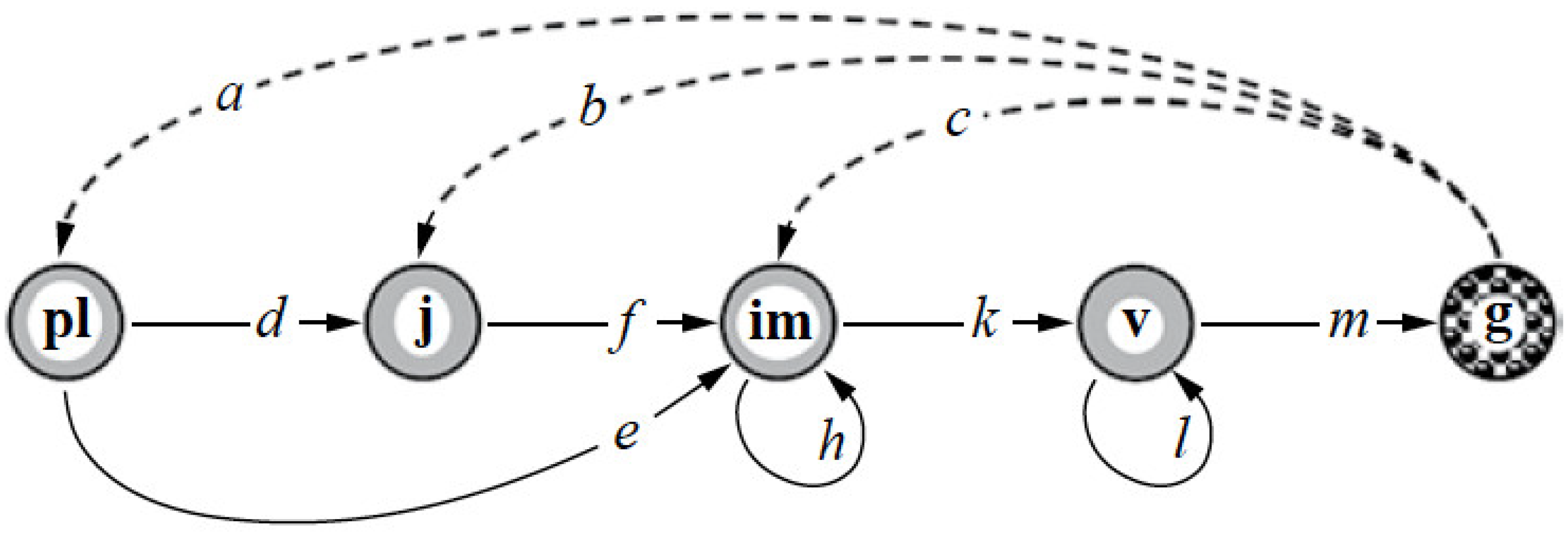
The pattern of matrix L shows the allocation of zero/nonzero elements in the matrix. It corresponds to the associated directed graph [2] called the life cycle graph (LCG) [1] as it represents graphically the knowledge of life histories involved into the model in combination with the way the population structure is observed in the field or laboratory (Figure 1 gives an example). If matrix L is positive or L = 0, then its pattern is trivial. When the LCG is strongly connected [2], it signifies a certain integrity of the individuals’ life history and provides for the PPM being irreducible [3,4]. However, the LCG ceases to be strong when it includes post-reproductive stages (a further, more complicated sample follows).

In theoretical layouts and practical applications, it is convenient to consider the PPM as the sum,

L = T + F,

(2)

of its parts that are responsible for the transitions (T) between individual statuses and population recruitment (F) [1,6]. In particular, if we number the graph nodes in Figure 1 from left to right, then we have

$$\mathit{L}=\mathit{T}+\mathit{F}=\left[\begin{array}{ccc}0& \begin{array}{cc}0& 0\end{array}& \begin{array}{cc}0& 0\end{array}\\ \begin{array}{c}d\\ e\end{array}& \begin{array}{cc}0& 0\\ f& h\end{array}& \begin{array}{cc}0& 0\\ 0& 0\end{array}\\ \begin{array}{c}0\\ 0\end{array}& \begin{array}{cc}0& k\\ 0& 0\end{array}& \begin{array}{cc}l& 0\\ m& 0\end{array}\end{array}\right]+\left[\begin{array}{ccc}0& \begin{array}{cc}0& 0\end{array}& \begin{array}{cc}0& a\end{array}\\ \begin{array}{c}0\\ 0\end{array}& \begin{array}{cc}0& 0\\ 0& 0\end{array}& \begin{array}{cc}0& b\\ 0& c\end{array}\\ \begin{array}{c}0\\ 0\end{array}& \begin{array}{cc}0& 0\\ 0& 0\end{array}& \begin{array}{cc}0& 0\\ 0& 0\end{array}\end{array}\right]$$

(3)

associated with the LCG shown in Figure 1. Matrix T is always column substochastic, i.e., its column sums do not exceed 1 according to their biological sense.

“When calibrated reliably from data, matrix L(t) gives rise to a rich repertoire of qualitative properties and quantitative indices characterizing the population under study at the place where and the time when the data were mined” ([7], p. 2/15). In particular, the dominant eigenvalue, λ₁(L) > 0, of matrix L, which coincides with ρ(L) (the spectral radius of L) and exists by the classical Perron–Frobenius theorem for nonnegative matrices [3,8,9], “gives a quantitative measure of how the local population is adapted to its environment [9], thus serving as an efficient tool of comparative demography [1] and enabling a forecast of population viability. This ability ensues from the dynamics of trajectory x(t) as t tends to +∞ when (a primitive [4]) L(t) = L does not change with time” ([7], p. 2/15). In formal terms, we have

$$\mathit{x}\left(t\right)~{{\lambda }_1}^t\mathit{x}*,\forall \mathit{x}\left(0\right)\in {ℝ}_{+}^n,$$

(4)

where x* is a positive eigenvector corresponding to λ₁, with a norm depending on x(0) [1]. Thus,

$$\mathit{x}(t)\to \{\begin{array}{c}\mathbf{0},\mathrm{if}{\lambda }_1<1;\\ x^{*},\mathrm{if}{\lambda }_1=1;\\ \infty ,\mathrm{if}{\lambda }_1>1,\end{array}$$

(5)

and the location of λ₁ relative to 1 may serve as a forecast of population viability if we believe that the vital rates do not change with t.

In practice, however, they do change quantitatively (yet retaining their single pattern) with time when t > 2. Each pair of consecutive years of observation generate a particular annual PPM L(t) obeying Equation (1) [1,5,10], and we have a finite set, L(0), L(1), …, L(M − 1), of M annual PPMs as a result of M + 1 observation years. Different PPMs generate different or even controversial (Table 3 in [9]) forecasts of population viability, and these motivate a task to average the set of PPMs in order to summarize all the years of observation.

1.2. Pattern-Multiplicative Average of Several PPMs

The logic behind averaging may be implicit or explicit and vary in complexity from the ordinariness of the arithmetic mean [11,12] through the weighted mean values of matrix elements [13] to the PMA concept [14] explained below.

Given a vector x(0) at the initial year of observation and a vector x(M) at the final year, it follows from (1) that

x(M) = L(M − 1) L(M − 2) … L(1) L(0) x(0),

(6)

i.e., the product of M annual PPMs (in the chronological order) transforms x(0) exactly to x(M). The logic of PMA suggests that the average matrix G should do exactly the same when raised to the Mth power. This is supposedly true for any observed vectors, whereby we conclude that

G^M = L(M − 1) L(M − 2) … L(1) L(0).

(7)

One more natural constraint on G consists in the pattern of G coinciding with that of the PPMs to be averaged.

Definition 1.

Let L(0), L(1), …, L(M − 1) be nonnegative square matrices with a single nontrivial pattern. Matrix G = G{L(0), L(1), …, L(M − 1)} is called the pattern-multiplicative average (or pattern-geometric average) of the M given matrices if it has the same pattern and obeys the averaging Equation (7).

Note that the vector-matrix Equation (7) with an n × n matrix G is equivalent to a system of n² scalar algebraic equations, and the question is how many unknown elements of G the system has to contain. When the pattern of G is trivially complete, i.e., when all the nonnegative matrices L(t) are actually positive, the number of unknowns equals n² as well, so that Equation (7) may have a nontrivial exact solution (Table 3 in [15]). However, when the pattern of L(t) is nontrivial, matching a real LCG, the number (k) of unknown positive entries in G is less than n², so that system (7) becomes an overdetermined system of algebraic equations (see, e.g., [16]). There is no reason to consider the remaining (n² − k) equations as a linear combination of the former k ones, so that the overdetermined system (7) is inconsistent and has no exact solutions.

The task to average M given PPMs can therefore be accomplished as an approximate solution to system (7), with a logical requirement to minimize the approximation error, which is measured in some reasonable way.

Definition 2.

Let L(0), L(1), …, L(M − 1) be nonnegative square matrices with a single nontrivial pattern. Matrix G = G{L(0), L(1), …, L(M − 1)} is called an approximate pattern-multiplicative average (APMA) of the M given matrices if it has the same pattern and represents a solution to a constrained minimization problem for the approximation error in solving system (7).

In what follows, we use the same notation G for the APMA matrix.

1.3. Minimization Problem for the Approximation Error

Equation (7) is obviously equivalent to

G^M − L(M − 1)L(M − 2) … L(1) L (0) = 0,

(8)

so that a norm of the left-hand side can be considered as the approximation error when G is an approximate solution rather than the exact one. When the matrix size (n × n) and the number of cofactors (M) are not too high, e.g., n = 5, M = 7 in Figure 1 and Equation (3), the APMA problem can be solved numerically by means of a modern software system such as MATLAB^® with an acceptable accuracy (Tables 3 and 4 and Appendix A in [5]).

However, the standard MATLAB tools return very rough estimates for higher dimensions n. This is seen, for example, in the sample calculations with n = 11 and M = 12. This phenomenon is quite natural since the error function is highly non-convex, in which case the optimization problem is notoriously hard. The number of local minima can grow exponentially with n. Therefore, the standard computer optimization software suffers when n is relatively large. In this case, one needs to choose special mathematical tools suitable for a particular problem. We find those tools as combinations of modern algorithms for local and global optimization.

2. Objects and Methods

2.1. A. albana Annual PPMs

Note that annual PPMs (3) contain 10 nontrivial elements a, b, …, l, m (called vital rates [1]), and if we consider them as a row vector, then the 12 annual PPMs of A. albana can be presented as a single table (

Table 1. Vital rates of A. albana as the entries of 12 annual PPMs (extracted from Table 3 in [10]).

Year	a	b	c	d	e	f	h	k	l	m
2009	30/13	40/13	3/13	8/37	2/37	22/110	28/29	7/99	19/35	1/35
2010	19/1	31/1	0/1	14/30	4/30	22/48	17/55	34/55	23/26	1/26
2011	49/1	85/1	25/1	1/19	6/19	35/45	21/43	10/43	48/57	7/57
2012	19/4	136/4	1/4	1/49	10/49	45/86	39/87	28/87	45/58	6/58
2013	16/6	98/6	2/6	0	2/19	16/137	14/95	6/95	64/73	3/73
2014	4/3	19/3	0/3	0	2/16	2/98	6/34	4/34	16/50	4/50
2015	10/4	29/4	0/4	0	0	10/19	3/10	5/10	17/20	1/10
2016	3/2	8/2	0	0	2/10	5/29	5/13	8/13	20/22	1/22
2017	12/1	23/1	0	0	3/3	2/8	8/12	2/12	21/28	2/28
2018	13/2	38/2	0	0	1/12	1/23	0/13	1/13	22/23	1/23
2019	8/2	9/9	0	1/3	2/3	2/3	4/4	2/4	19/19	5/19
2020	8/2	9/2	0	1/3	2/3	2/3	4/4	1/13	19/19	5/15

). Those rates take on the form of rational numbers according to the way they were mined in the field [5].

We consider solving the APMA problem for the first 7 PPMs (2009–2015) as Example 1 and for all the 12 ones as Example 4. Example 2 will refer to the seven matrices modified in some elements as marked in

Table 2. Example 2: modified Example 1 for testing the column substochastic property.

“Year”	a	b	c	d	e	f	h	k	l	m
1	30/13	4/13	3/13	8/37	2/37	22/110	28/29	7/99	9/35	11/35
2	19/1	31/1	0/1	14/30	4/30	22/48	17/55	34/55	25/26	1/26
3	49/1	85/1	25/1	1/19	6/19	35/45	21/43	10/43	48/57	7/57
4	19/4	136/4	1/4	1/49	10/49	45/86	39/87	28/87	45/58	8/58
5	16/6	98/6	2/6	0	2/19	16/137	14/95	6/95	64/73	3/73
6	4/3	19/3	0/3	0	2/16	2/98	6/34	4/34	16/50	26/50
7	10/4	29/4	0/4	0	0	10/19	3/10	5/10	17/20	1/10

with bold.

2.2. Calamagrostis epigeios PPM and Its Perturbations

C. epigeios is a long-rhizome perennial graminoid actively colonizing open areas in the temperate zone [17]. Its biology is well studied, and the life cycle graph was constructed in terms of both ontogenetic stage and chronological age (Figure 2). In contrast to Figure 1, the C. epigeios digraph is not strongly connected, but it contains what was called the reproductive core of the LCG, the maximal connected subgraph [13].

The construction was based on the data gained by excavating a whole local colony of the plants [17]. Those data enabled calibrating a single PPM alone. The entries of the transition part were determined in a unique way as rational numbers, while those of the 5 × 5 reproductive-core submatrix remained uncertain:

$$\mathit{L}=\left[\begin{array}{ccccccccccc}a/43& b/7& 0& c/12& d/3& 0& e/3& 0& 0& 0& 0\\ 23/43& 0& 0& 0& 0& 0& 0& 0& 0& 0& 0\\ 0& 0& 0& 0& 0& 0& 0& 0& 0& 0& 0\\ f/43& 0& 0& 0& g/3& 0& h/3& 0& 0& 0& 0\\ 10/43& 0& 0& 7/12& 0& 0& 0& 0& 0& 0& 0\\ k/43& 0& 0& 0& 0& 0& 0& 0& 0& 0& 0\\ 2/43& 0& 0& 1/12& 0& 0& 0& 0& 0& 0& 0\\ 0& 0& 0& 0& 0& 0& 2/3& 0& 0& 0& 0\\ 1/43& 0& 0& 0& 0& 0& 0& 0& 0& 0& 0\\ 0& 0& 0& 0& 0& 0& 0& 0& 0& 0& 0\\ 0& 2/7& 0& 0& 2/3& 0& 0& 0& 0& 0& 0\end{array}\right],$$

(9)

restricted with certain linear equalities (“reproductive uncertainty” [17], p. 387):

$$\{\begin{array}{c}a+b+c+d+e=163,\\ f+g+h=22,\end{array}$$

(10)

and certain linear inequalities:

a + f + k ≥ c + g ≥ d + h ≥ b ≥ e,

(11)

ensued from the expert knowledge [17]. Here, the 9 reproduction rates a, b,…, h, k ≥ 0 take on integer values only in accordance with empirical data [17]: after the Colony had been excavated and all the mother-daughter rhizome links counted, the 9 uncertain parameters became certain (ibidem,

Table 3. Example 3: Nonzero elements of the 9 Calamagrostis epigeios PPMs to be averaged.

“Year”	a	b	c	d	e	f	g	h	k	λ1
1	117	3	38	3	2	12	9	1	1	3.4266
2	100	2	54	5	2	12	8	2	2	3.3093
3	120	3	36	2	2	14	7	1	5	3.4198
4	125	4	30	2	2	10	10	2	2	3.4707
5	117	1	41	3	1	10	10	2	1	3.4124
6	119	2	37	3	2	13	7	2	3	3.4050
7	123	3	34	1	2	11	9	2	1	3.4281
8	106	5	45	4	3	12	9	1	2	3.3740
9	111	3	45	3	1	10	10	2	1	3.3847

) and resulted in λ₁(L) = 3.4266 (ibidem) signifying rapid growth of the young Colony.

To illustrate the concept of PMA we have to obtain a finite set of such matrices, and we have obtained it by means of perturbing the nine rates artificially to the values presented in Table 3 (“years” 2 to 9) together with the corresponding values of λ₁(L).

2.3. Mathematical Problem Formulation

We solve the following APMA problem:

$$\begin{gathered} \{\begin{array}{c}f\left(\mathit{X}\right)=\parallel {\mathit{X}}^M-{\mathit{L}}_M\dots {\mathit{L}}_1{\parallel }_F\to mi{n}_{\mathit{X}},\\ mi{n}_k^{+}{\mathit{L}}_k\left(i,j\right)\le X\left(i,j\right)\le ma{x}_k{\mathit{L}}_k\left(i,j\right),i,j=1,\dots ,n;\end{array} \\ mi{n}_{}^{+}\left(x,y\right)=\{\begin{array}{c}min\left(x,y\right)ifx·y\ne 0,\\ max\left(x,y\right)ifx·y=0,\end{array} \end{gathered}$$

(12)

where the n × n matrix X has a prescribed pattern (the allocation of nonzero elements) and the expression

$${\parallel \mathit{X}\parallel }_F=\sqrt{x_{11}^2+\dots +x_{nn}^2}$$

(13)

denotes the Frobenius norm of the matrix. Additional linear constraints on the elements of X (both equalities and inequalities) can also be incorporated, such as conditions (10)–(11) and those of the transition part in (3) being substochastic.

Instead of minimizing the “loss function” (in the terminology of optimization theory) f(X) = $\parallel {\mathit{X}}^M-{\mathit{L}}_M{\mathit{L}}_{M-1}\dots {\mathit{L}}_2{\mathit{L}}_1{\parallel }_F$, we may consider minimizing the loss function Φ(X) = f²(X) that is calculated as the sum of all the squared elements in the difference of two matrices. The minimum has to be reached at the same matrix X.

2.4. Method 1 to Solve the APMA Problem

We use the basin-hopping method of global optimization suggested in [18,19,20]. This is an iterative stochastic method reduced to repeating three key steps. First, the coordinates are randomly perturbed, and a method of local optimization is then launched from the perturbed starting point. Finally, based on the obtained minimum, it is determined whether the coordinate perturbation has turned out to be successful and has to be saved. The base version of the basin-hopping method uses the Metropolis criterion algorithm [21], although modifications are also possible.

To find a local minimum, we use the trust-region method (TRM) suggested in [22,23] as the algorithm of local optimization. It first determines a trust region around the best current solution, and a quadratic model of approximation is then used within this region. The region size is updated at each step, i.e., the size increases if the approximation of the objective function is rather good; otherwise, it decreases. Trust-region methods are quite popular in solving various nonlinear optimization problems due to their applicability to the ill-conditioned ones and to their convergence and robustness properties; see [24] and references therein.

TRM methods support both the equality- and inequality-type constraints, and they guarantee the constraints to hold after optimization (in contrast to other local methods such as SLSQP or L-BFGS [25]). However, the TRM may sometimes be slower, and the alternative methods of local optimization could also be useful in some cases.

2.5. Method 2 to Solve the APMA Problem

The second approach originates from the class of penalty methods. In these methods, an additional term is introduced as a measure of constraint violations. In our case, we consider the column substochastic constraints and solve the following problem:

$$\{\begin{array}{c}\parallel {\mathit{X}}^M-{\mathit{L}}_M\dots {\mathit{L}}_1{\parallel }_2^2+\epsilon \left(\mathit{X}\right)\to mi{n}_{\mathit{X}};\\ mi{n}_k^{+}{\mathit{L}}_k\left(i,j\right)\le X\left(i,j\right)\le ma{x}_k{\mathit{L}}_k\left(i,j\right),i,j=1,\dots ,n,\end{array}$$

(14)

where ε(X) consists of several summands, each one corresponding to one of the inequalities. If an inequality is violated, the corresponding summand equals the squared magnitude of violation multiplied with a constant. For example, when the inequality is X(0, 0) + X(0, 1) ≤ 1, the summand equals C (X(0, 0) + X(0, 1) − 1) ² if X(0, 0) + X(0, 1) > 1.

Constant C should be chosen manually as its value depends on the current state of the algorithm. It is a popular strategy to change the value of C in the course of the algorithm because smaller Cs are better at the beginning phase, as they accelerate the convergence of the gradient descent. However, larger values of C are desirable in the end of the algorithm since they guarantee the feasibility of constraints.

We have seen in experiments that it is better not to put any box constraints in the penalty summands, but rather to diversify them as the bounds for the variables.

The basin-hopping algorithm described above (Section 2.4) can be used as a global optimization method. If we do not have any additional constraints of equality type, then the choice of the underlying local methods becomes wider. For example, it is possible to use the L-BFGS algorithm [26], which is faster than the TRM. If, however, we do have additional equality constraints, the TRM shall still be used.

We suggest another problem setting in the next section, where we minimize another loss function, the same methods still being applicable there. Both Method 1 and Method 2 work more stably when the derivatives of their loss functions are given explicitly. They are calculated for the both loss functions in the next Section.

3. New Loss Function of Approximation

Introduced in Section 2.3 as a measure of approximation error, the loss function Φ(X) has several disadvantages. First, it measures the absolute error and changes with the normalization of matrices. A suitable normalization can be done by the division by the norm of the matrix, or by the spectral radius product of the product L_M … L₁. However, normalization cannot exclude other shortcomings, either. Some of them are explained below.

(1)

Loss function Φ behaves differently in the approximations from above and from below. This phenomenon already occurs in the dimension n = 1. In the one-dimensional case, we denote the “matrices” (numbers) with small letters. Let x be an approximation of the multiplicative mean of numbers l_M, …, l₁. Denote q = (l_M … l₁)^1/M; then Φ(x) = |x^M − q^M|². Normalize all the l_j such that q = 1 and note a key difference between the cases of x < 1 and x > 1, namely,

$$\Phi (x)\{\begin{array}{c}\to \infty \mathrm{as}M\to \infty \mathrm{if}x>1,\\ <1\mathrm{for}\mathrm{all}M\mathrm{if}x<1.\end{array}$$

Let, for example, M = 10. When x = 1.1, we have Φ(x) = |x¹⁰ − 1|² = 2.54. On the other hand, for x = 0.1, we have Φ(x) = |0.1¹⁰ − 1|² = 0.9999…, hence the loss function Φ has to choose the approximation x = 0.1 in spite of it being much worse.

(2)

The value of Φ may increase with M and even tend to infinity. In the example above, if x = 1.1, we have Φ(x) → ∞ as M → ∞. In real practice, however, the situation should be the opposite: the greater M, the sharper will be the approximation to the average value.

(3)

When ρ(X), the spectral radius of X is small, and the value of Φ can be very small and unable to distinguish the quality of approximation. In the example above, when M = 100, the approximations x = 0.5 and x = 0.1 are practically not comparable because Φ(x) < 10⁻³⁰ in both cases.

The following idea helps avoid all of these shortcomings. In the case of n = 1, if q denotes the actual value of the multiplicative mean and x our approximation, then

$$|x-q{|}^2=\frac{{|x^M-q^M|}^2}{{|q^{M-1}+q^{M-2}x+\dots +q{x}^{M-2}+x^{M-1}|}^2}$$

(15)

Thus, the numerator Φ(x) is divided by a specially chosen denominator. If q is unknown, the powers q^k can be replaced by the products l_M … l_{M −k+1}. The same principle can be applied in our problem, when we deal with matrices instead of numbers. We begin with l_M since this is chronologically the last measurement and it should give the main contribution to measuring the quality of approximation when the application context suggests such a priority. Translating this idea to the general dimension n, we replace Φ with the new loss function S(X) = s(X)²:

$$S(\mathit{X})=\frac{\Phi \left(\mathit{X}\right)}{\Psi \left(\mathit{X}\right)},$$

(16)

where Ψ is defined as

$$\Psi (\mathit{X})=\parallel {{\displaystyle \sum }}_{j=0}^{M-1}{\mathit{L}}_M\dots {\mathit{L}}_{j+2}{\parallel }^2$$

(17)

We derive the derivative of Ψ by applying Proposition 1 (see Appendix A):

$$S^{\prime }(\mathit{X})=\frac{\Psi {\Phi }^{\prime }-\Phi {\Psi }^{\prime }}{{\Psi }^2},$$

(18)

where Φ = Φ(X), Ψ = Ψ(X) are defined in (A.1) and the derivatives Φ’, Ψ ’ are derived by the formulas from Proposition 1. Note that Φ’, Ψ ’ are n × n matrices, while Φ and Ψ are nonnegative numbers, Ψ ≠ 0. That is why the division in (18) is well defined and Ψ commutes with Φ’.

4. Results

In this section, we report on the numerical results obtained by the methods presented in Section 2.4, Section 2.5 and Section 3 and applied to the Examples listed in Section 2.1, Section 2.2 and Section 2.3. We consider settings with both the loss function Φ(X) = f(X)² (12) and S(X) = s(X)² (16), both being calculated in each example for the purpose of comparison (

Table 4. Results for Example 1.

Method	$\mathit{f}(\widehat{\mathit{X}})$	$\mathit{s}(\widehat{\mathit{X}})$	$\mathit{\rho }(\widehat{\mathit{X}})$	$\widehat{\mathit{X}}$
Method 1 with Φ(X)	0.02109	0.002374	0.8585	0	0	0	0	3.3309
				0.453	0	0	0	7.8767
				0.0288	0.2936	0.1474	0	0
				0	0	0.1726	0.7589	0
				0	0	0	0.1034	0
Method 2 with Φ(X)	0.021089	0.002374	0.8585	0	0	0	0	3.3309
				0.4533	0	0	0	7.8757
				0.0287	0.22936	0.1474	0	0
				0	0	0.1726	0.7589	0
				0	0	0	0.1034	0
Method 1 with S(X)	0.021176	0.002379	0.8584	0	0	0	0	3.3348
				0.4322	0	0	0	7.9666
				0.0363	0.2897	0.1485	0	0.0022
				0	0	0.1728	0.7587	0
				0	0	0	0.1034	0

,

Table 5. Results for Example 2.

Method	$\mathit{f}(\widehat{\mathit{X}})$	$\mathit{s}(\widehat{\mathit{X}})$	$\mathit{\rho }(\widehat{\mathit{X}})$	$\widehat{\mathit{X}}$
Method 1 with Φ(X)	2.865725	0.01689	0.8952	0	0	0	0	29.9759
				0	0	0	0	85
				0.1383	0.0204	0.1474	0	0.1929
				0	0	0.1095	0.32	0
				0	0	0	0.52	0
Method 2 with Φ(X)	2.865725	0.016890	0.8952	0	0	0	0	29.9759
				0	0	0	0	85
				0.1383	0.0204	0.1474	0	0.1929
				0	0	0.1095	0.32	0
				0	0	0	0.52	0
Method 1 with S(X)	2.874438	0.016851	0.8968	0	0	0	0	30.7974
				0.0002	0	0	0	84.9995
				0.1033	0.0344	0.1474	0	0.2694
				0	0	0.1053	0.3201	0
				0	0	0	0.52	0

, Table 6 and Table 7).

Technical parameters are as follows: in Method 1, we have used 20 iterations of the basin-hopping algorithm; in Method 2, the first 80 iterations have been made with C = 40, and the next 20 with C = 2040.

Next, we demonstrate the numerical results for Example 2, an artificial example to analyze the sensitivity of our method to the substochasticity constraint. The numerical experiments (see Table 5) show that the results may change after imposing that the solution must be a column substochastic matrix.

The results for Example 3 turn out to be the same and independent of the linear inequalities. Using Method 2 makes no sense in this case as the linear equalities (10) suggest using the TRM. Note that without linear inequalities, Method 2 is the same as Method 1.

5. Discussion

To realize our goal of finding the multiplicative mean of several PPMs, we note first that this problem may have an exact solution. For example, if the matrix product is diagonalizable, then the multiplicative mean is a diagonal matrix too in the appropriate basis, with the elements being the complex roots of the corresponding power from the diagonal elements of the original matrix product. The solution is not unique because of the non-uniqueness of the complex roots. Taking any of the solutions and transferring back to the original basis, we get a multiplicative mean. This mean, however, may not be a nonnegative matrix. Even if it is, it may not satisfy our imposed constraints. This argument, in addition to that one in Section 1.2 concerning the lack of exact solutions to Equation (7), substantiates the approximation approach to the problem of pattern-multiplicative average.

We search for a matrix satisfying all the constrains and being close to the unknown pattern-multiplicative average, G, by means of some loss function. This leads to optimization problem (13), where the loss function is the Frobenius norm. The Frobenius norm is the most popular one in matrix analysis since it is actually the Euclidean norm in the space of matrices equipped with the standard scalar product. However, this choice of the distance has several disadvantages, as noted in Section 3. We introduce a modified loss function and obtain another optimization problem. Both problems are not easy to solve as they are highly non-convex, and hence may possess many local extrema, and because of a large number of variables. Non-convexity implies all the known optimization methods to converge only to local extrema. Therefore, we use the following strategy: first we get a rough approximation to the optimum by using the global optimization tools, then we improve the solution by searching for a close point of local minimum (hoping that this local minimum is close to the global one). Among all the global optimization methods we choose the basing-hopping method since it successfully approximates the optimal value for problems with linear constraints even in relatively high dimensions. The next step, i.e., improving the solution with a close local minimum, can be realized by various popular algorithms: the Newton method, gradient methods, the Frank–Wolf algorithm, the trust region method (TRM), etc. Most of them need a relatively small Lipschitz constant for the gradient, which is not always the case (see the explicit formulas of the gradient in Appendix A). That is why the TRM is the most efficient algorithm for our problem.

Despite theoretical disadvantages of the loss function Φ noted in Section 3, our practical calculations have revealed only minor improvements that the alternative S brings with any method of the optimal search.

It is easy to see that the arithmetic mean of all the nine perturbed λ₁s (Table 3) equals 3.4034. Neither the arithmetic mean of the annual λ₁s, nor λ₁ of the arithmetic average of the annual PPMs can even serve as a crude estimate of the λ₁(G).

Note that we do not pretend to exhaust here the theme of “versatile optimization tools”. For example, a penalty method that can reduce a non-convex problem to an infinite-dimensional optimal control problem [27] or the generalized subdiffenential technique based on the sequential optimality conditions [28] look fairly perspective, too. Some non-convex optimization problems related to the matrix calculus also appear naturally in the approximation problems, for example, the barycentric rational polynomial approximation [29] and the generalized weak greedy approximation [30].

Coming back to the logic of PMA, consider the equation

G^M = ProdL

(19)

equivalent to (8) if ProdL denotes the product of M matrices in its left-hand side. Since λ₁(G ^M) = λ₁(G )^M, it follows from (19) that the exact value of λ₁(G),

λ₁(G) = [λ₁(ProdL)]^1/M,

(20)

is quite calculable from the data and equal to 3.4017 in Example 3 (M = 9), to 0.893087 in Example 4 (M = 12). It should not be surprising therefore that the corresponding optimized values of ρ(X) = 3.41... (Table 6) and = 0.88… (Table 7) are close to the exact ones above. Not surprising would also be an alternative formulation of the APMA problem suggesting the difference between λ₁s as the loss function. Optimization along this line or even that in combination with the former loss function is worthy of further research efforts.

Table 6. Results for Example 3.

Method	$\mathit{f}(\widehat{\mathit{X}})$	$\mathit{s}(\widehat{\mathit{X}})$	$\mathit{\rho }(\widehat{\mathit{X}})$	$\widehat{\mathit{X}}$
Method 1 with Φ(X)	8244.621552	0.0292	3.4118	2.6026	0.4901	0	3.4104	1.3229	0	0.9206
				0.5349	0	0	0	0	0	0
				0	0	0	0	0	0	0
				0.2558	0	0	0	3.3333	0	0.3333
				0.2326	0	0	0.5833	0	0	0
				0.0233	0	0	0	0	0	0
				0.0465	0	0	0.0833	0	0	0
Method 1 with S(X)	8257.167555	0.029157	3.4107	2.5953	0.4891	0	3.4287	1.35	0	0.928
				0.5349	0	0	0	0	0	0
				0	0	0	0	0	0	0
				0.2558	0	0	0	3.3332	0	0.3334
				0.2326	0	0	0.5833	0	0	0
				0.0237	0	0	0	0	0	0
				0.0465	0	0	0.0833	0	0	0

Table 6. Results for Example 3.

Method	$\mathit{f}(\widehat{\mathit{X}})$	$\mathit{s}(\widehat{\mathit{X}})$	$\mathit{\rho }(\widehat{\mathit{X}})$	$\widehat{\mathit{X}}$
Method 1 with Φ(X)	8244.621552	0.0292	3.4118	2.6026	0.4901	0	3.4104	1.3229	0	0.9206
				0.5349	0	0	0	0	0	0
				0	0	0	0	0	0	0
				0.2558	0	0	0	3.3333	0	0.3333
				0.2326	0	0	0.5833	0	0	0
				0.0233	0	0	0	0	0	0
				0.0465	0	0	0.0833	0	0	0
Method 1 with S(X)	8257.167555	0.029157	3.4107	2.5953	0.4891	0	3.4287	1.35	0	0.928
				0.5349	0	0	0	0	0	0
				0	0	0	0	0	0	0
				0.2558	0	0	0	3.3332	0	0.3334
				0.2326	0	0	0.5833	0	0	0
				0.0237	0	0	0	0	0	0
				0.0465	0	0	0.0833	0	0	0

Table 7. Results for Example 4.

Method	$\mathit{f}(\widehat{\mathit{X}})$	$\mathit{s}(\widehat{\mathit{X}})$	$\mathit{\rho }(\widehat{\mathit{X}})$	$\widehat{\mathit{X}}$
Method 1 with Φ(X)	0.045898	0.007149	0.8876	0	0	0	0	2.7782
				0. 1508	0	0	0	3.0007
				0.1125	0.3106	0	0	0.8163
				0	0	0.3105	0.7453	0
				0	0	0	0.1515	0
Method 2 with Φ(X)	0.05156	0.008283	0.8863	0	0	0	0	3.3354
				0.3108	0	0	0	3
				0.0591	0.3165	0.1474	0	0.6754
				0	0	0.2577	0.7682	0
				0	0	0	0.1257	0
Method 1 with S(X)	0.046195	0.00708	0.888	0	0	0	0	2.6526
				0.0041	0	0	0	3.3033
				0.1436	0.2818	0.0001	0	0.8541
				0	0	0.3193	0.7378	0
				0	0	0	0.1588	0

Table 7. Results for Example 4.

Method	$\mathit{f}(\widehat{\mathit{X}})$	$\mathit{s}(\widehat{\mathit{X}})$	$\mathit{\rho }(\widehat{\mathit{X}})$	$\widehat{\mathit{X}}$
Method 1 with Φ(X)	0.045898	0.007149	0.8876	0	0	0	0	2.7782
				0. 1508	0	0	0	3.0007
				0.1125	0.3106	0	0	0.8163
				0	0	0.3105	0.7453	0
				0	0	0	0.1515	0
Method 2 with Φ(X)	0.05156	0.008283	0.8863	0	0	0	0	3.3354
				0.3108	0	0	0	3
				0.0591	0.3165	0.1474	0	0.6754
				0	0	0.2577	0.7682	0
				0	0	0	0.1257	0
Method 1 with S(X)	0.046195	0.00708	0.888	0	0	0	0	2.6526
				0.0041	0	0	0	3.3033
				0.1436	0.2818	0.0001	0	0.8541
				0	0	0.3193	0.7378	0
				0	0	0	0.1588	0

6. Conclusions

We solve the problem of finding a matrix of a special pattern which is close, in a certain sense, to the multiplicative mean of several given matrices. The closeness is measured by a loss function, which is usually non-convex and may have a large Lipschitz constant of the derivative. This makes the problem of finding the optimal matrix, i.e., of minimizing the loss function, very difficult. We have elaborated a two-phase method for this problem. The first phase realizes a rough search of the absolute minimum, and this is done by the basing-hopping method of global optimization. The second phase provides for an improved solution at a point of local minimum in a vicinity of our global solution, and this is done by the trust region method. In numerical examples, we demonstrate the efficiency of our strategy even for relatively high dimensions. Implementation of these ideas in the problem of pattern-multiplicative average is not direct and requires the overcoming of some technical obstacles, which have nevertheless been bypassed in this study. While the traditional approach to global optimization reduces to searching for the best solution among the local ones found preliminary, the nontraditional inverted logic may be successful when the direct one fails.

References

1. Caswell, H. Matrix Population Models: Construction, Analysis and Interpretation, 2nd ed.; Sinauer Associates: Sunderland, MA, USA, 2001. [Google Scholar]
2. Harary, F.; Norman, R.Z.; Cartwright, D. Structural Models: An Introduction to the Theory of Directed Graphs; John Wiley: New York, NY, USA, 1965. [Google Scholar]
3. Gantmacher, F.R. Matrix Theory; Chelsea Publ.: New York, NY, USA, 1959. [Google Scholar]
4. Horn, R.A.; Johnson, C.R. Matrix Analysis; Cambridge University Press: Cambridge, UK, 1990. [Google Scholar]
5. Logofet, D.O.; Kazantseva, E.S.; Belova, I.N.; Onipchenko, V.G. How long does a short-lived perennial live? A modelling approach. Biol. Bul. Rev. 2018, 8, 406–420. [Google Scholar] [CrossRef]
6. Cushing, J.M.; Yicang, Z. The net reproductive value and stability in matrix population models. Nat. Res. Model. 1994, 8, 297–333. [Google Scholar] [CrossRef]
7. Logofet, D.O.; Razzhevaikin, V.N. Potential-growth indicators revisited: Higher generality and wider merit of indication. Mathematics 2021, 9, 1649. [Google Scholar] [CrossRef]
8. Seneta, E. Non-Negative Matrices; Wiley: New York, NY, USA, 1973. [Google Scholar]
9. Berman, A.; Plemmons, R.J. Nonnegative Matrices in the Mathematical Sciences; Academic: New York, NY, USA, 1979. [Google Scholar]
10. Logofet, D.O.; Kazantseva, E.S.; Belova, I.N.; Onipchenko, V.G. Backward prediction confirms the conclusion on local plant population viability. Biol. Bul. Rev. 2021, 11, 406–420. [Google Scholar] [CrossRef]
11. Klimas, C.A.; Cropper, W.P., Jr.; Kainera, K.A.; de Oliveira Wadt, L.H. Viability of combined timber and non-timber harvests for one species: A Carapa guianensis case study. Ecol. Model. 2012, 246, 147–156. [Google Scholar] [CrossRef]
12. Logofet, D.O. Projection matrices in variable environments: λ1 in theory and practice. Ecol. Model. 2013, 251, 307–311. [Google Scholar] [CrossRef]
13. Maslov, A.A.; Logofet, D.O. Joint population dynamics of Vaccinium myrtillus and V. vitis-idaea in the protected postfire Cladina-Vaccinium pine forest. Markov model with averaged transition probabilities. Biol. Bul. Rev. 2021, 11, 406–420. [Google Scholar] [CrossRef]
14. Logofet, D.O. Averaging the population projection matrices: Heuristics against uncertainty and nonexistence. Ecol. Complex. 2018, 33, 66–74. [Google Scholar] [CrossRef]
15. Logofet, D.O.; Maslov, A.A. Analyzing the fine-scale dynamics of two dominant species in a Polytrichum–Myrtillus pine forest. II. An inhomogeneous Markov chain and averaged indices. Biol. Bul. Rev. 2019, 9, 62–72. [Google Scholar] [CrossRef]
16. Anton, H.; Rorres, C. Elementary Linear Algebra, 9th ed.; Wiley: Hoboken, NJ, USA, 2005. [Google Scholar]
17. Logofet, D.O.; Ulanova, N.G.; Belova, I.N. From uncertainty to an exact number: Developing a method to estimate the fitness of a clonal species with polyvariant ontogeny. Biol. Bull. Rev. 2017, 7, 387–402. [Google Scholar] [CrossRef]
18. Wales, D.J.; Doye, J.P.K. Global optimization by basin-hopping and the lowest energy structures of Lennard-Jones clusters containing up to 110 atoms. J. Phys. Chem. A 1997, 101, 5111–5116. [Google Scholar] [CrossRef] [Green Version]
19. Conn, A.R.; Gould, N.I.M.; Toint, P.L. Trust Region Methods; MOS-SIAM Series on Optimization; Society for Industrial and Applied Mathematics: Philadelphia, PA, USA, 2000. [Google Scholar] [CrossRef]
20. Vinkó, T.; Gelle, K. Basin Hopping Networks of continuous global optimization problems. Cent. Eur. J. Oper Res. 2017, 25, 985–1006. [Google Scholar] [CrossRef] [Green Version]
21. Robert, C.P.; Casella, G. Monte Carlo Statistical Methods, 2nd ed.; Springer: New York, NY, USA, 2004. [Google Scholar] [CrossRef] [Green Version]
22. Sorensen, D.C. Newton’s method with a model trust region modification. SIAM J. Numer. Anal. 1982, 19, 409–426. [Google Scholar] [CrossRef] [Green Version]
23. Yuan, Y. A review of trust region algorithms for optimization. In Proceedings of the 4th International Congress on Industrial & Applied Mathematics (ICIAM 99), Edinburgh, UK, 14 December 2000; pp. 271–282. [Google Scholar]
24. Sun, W.; Yuan, Y.-X. Optimization Theory and Methods: Nonlinear Programming; Springer: New York, NY, USA, 2006; Available online: https://books.google.ru/books?id=o0BYHLhhPJMC (accessed on 21 October 2022).
25. Jorge Nocedal, J.; Wright, S.J. Numerical Optimization; Springer: New York, NY, USA, 2006. [Google Scholar]
26. Liu, D.C.; Nocedal, J. On the limited memory BFGS method for large scale optimization. Math. Program. 1989, 45, 503–528. [Google Scholar] [CrossRef] [Green Version]
27. Hammoudi, A.; Benharrat, M. An exact penalty method for constrained optimal control problems. Rend. Circ. Mat. Palermo Ser. 2 2021, 70, 275–293. [Google Scholar] [CrossRef]
28. Moustaid, M.B.; Rikouane, A.; Dali, I.; Laghdir, M. Sequential approximate weak optimality conditions for multiobjective fractional programming problems via sequential calculus rules for the Brøndsted-Rockafellar approximate subdifferential. Rend. Circ. Mat. Palermo Ser. 2 2022, 71, 737–754. [Google Scholar] [CrossRef]
29. Li, J. Linear barycentric rational collocation method for solving biharmonic equation. Demonstr. Math. 2022, 55, 587–603. [Google Scholar] [CrossRef]
30. Valiullin, A.R.; Valiullin, A.R.; Solodov, A.P. Sharp sufficient condition for the convergence of greedy expansions with errors in coefficient computation. Demonstr. Math. 2022, 55, 254–264. [Google Scholar] [CrossRef]
Figure 1. Life cycle graph for a local population of Androsace albana, an alpine short-lived perennial species, observed once a year. Ontogenetic stage notations: pl, seedlings; j, juvenile plants; im, immature plants; v, adult vegetative plants; g, generative plants, the stages being distinguishable in the field. Solid arrows indicate transitions occurring for one year (no transition, in particular); dashed arrows correspond to the annual population recruitment [5].
Mathematics 10 04417 g001
Figure 2. LCG for Calamagrostis epigeios according to the excavation data of a 3-year-old colony in 2015: v denotes the stage of adult vegetative plants; gi (i = 1, 2, 3), generative plans with i generative shoots; ss and s, subsenile and senile stages, respectively. Solid arrows indicate the ontogenetic transitions that have occurred for 1 year: numbers at the arrows indicate proportions of the tufts outgoing from an initial status in 2014 and reaching the ingoing status by 2015; the number inside the vertex is the ordinal number the corresponding component has in the vector of population structure; gray background highlights the reproductive core of the LCG (Figure 4I in [17]).
Mathematics 10 04417 g002