Local Non-Similar Solutions for Boundary Layer Flow over a Nonlinear Stretching Surface with Uniform Lateral Mass Flux: Utilization of Third Level of Truncation

Abstract

The present study aims to examine the effects of uniform lateral mass flux on the boundary layer flow induced by a non-linearly stretching surface. For uniform mass flux, the boundary layer flow does not conform to a similarity solution. The problem may be resolved by the similarity solution only when the transverse velocity at the boundary of the porous stretching surface is of the form $v_w\sim x^{\frac{p-1}{2}}.$ In other words, the flow becomes non-similar; to date, this has not been reported in the literature. That is why, in the current study, the local-similarity approximation up to the third level of truncation is utilized to solve the problem. The pseudo-similarity variable, stream function and transformed streamwise coordinate are defined such that the continuity equation is identically satisfied, and the momentum equation reduces to a non-similar dimensionless boundary layer equation. We derived the non-similar equations of the first, second and third levels of truncations and compared the numerical results obtained from different levels of truncations. In order to find numerical solutions to these equations, the built-in MATLAB routine, known as bvp4c, is used. Further, all non-similar terms that appear in the momentum equations are retained without any approximations. The approximations are introduced only in the subsidiary equations and relative boundary conditions. For the case of suction, the rate of increase in the numerical values of skin friction coefficient obtained from the first level of truncation with increasing velocity index parameter is found to be underestimated, while overestimation is found in the case of injection. The numerical results that were obtained from the third level of truncations are plotted against the embedding physical parameters and are then discussed.

1. Introduction

The phenomenon of suction or blowing is of considerable practical significance in many applications and has been used effectively in transpiration cooling, energizing the inner boundary layer in an adverse pressure gradient, increasing the lift on aerofoils, preventing corrosion or scaling, and cooling of surfaces exposed to high-temperature flows. In drag reduction, suction is also used in chemical processes to remove reactants, while injection is applied to add reactants, to control boundary layers, etc. [1,2,3,4]. Boundary layer flows over a stretching surface have many engineering and industrial applications. Crane [5] was the first to investigate the flow of a boundary layer over a stretching surface. He opened a new direction for researchers, which have started working on the boundary layer flows induced by stretching surfaces to benefit industries involved in manufacturing processes like continuous casting, polymer extrusion, wire drawing, hot rolling, glass blowing, paper production, annealing and drawing of plastic films, fiber spinning, etc. [6,7,8,9,10,11,12]. The first attempt to analyze the effect of suction or injection (blowing) on the boundary layer flow over a linearly stretching surface was made by Gupta and Gupta [13]. They reported a similarity solution in the presence of constant mass suction/injection and observed that an increase in suction causes a gradual thinning of the boundary layer, whereas blowing has the opposite effect. Chen and Char [14] also investigated a linearly stretching surface subject to suction or injection. A few recent investigations on the flow over permeable (porous) linearly stretched sheets have been performed by [15,16,17,18,19,20,21,22]. Bank [23] firstly examined the flow over a nonlinear stretching (power law velocity variation of the form $U_0{x}^m$, here m is the velocity exponent parameter and $U_0$ is dimensional constant having dimension $\left[\left(length/time\right){\left(length\right)}^{-m}\right]$) and computed the similarity solutions numerically. Research by Vajravelu [24] focused on the investigation of fluid motion in conjunction with heat transfer while maintaining a constant temperature at the wall. Ali [25] extended the analysis reported in [13] from linear to non-linear stretching flow, and that in [14] by considering the porous stretching sheets instead of impermeable ones. They also analyzed the impact of suction or blowing on the boundary layer thickness and skin-friction coefficient. Ali [25] proposed that the suction/injection velocity $V_w\left(=\sqrt{\frac{\nu U_0}{x^{1-p}}}\right)$ in which $\left(V_w,U_0,x,p,\nu \right)$ respectively represent the vertical velocity component at the boundary, the dimensional constant, the Cartesian coordinate along the stretching boundary, the velocity index parameter and the kinematic viscosity, must be a function of the distance from the leading edge to permit similarity solutions. Hence, for the constant wall suction/blowing velocity, a similarity solution does not exist for the flow over a non-linearly stretching surface [26,27]. In some prior studies, the number of independent variables was not reduced after performing the proposed transformations, and a space variable $x$ appeared in the mass flux parameter. Researchers merged this space variable in the mass suction/injection parameter and treated this as constant velocity and the corresponding equations as locally self-similar, which actually corresponds to non-similar situations. The elementary flow quantities in non-similar boundary layer flow changes in a stream-wise direction. In summary, a more realistic scenario for the flow over a nonlinear porous stretching sheet would use uniform surface mass transfer [28]; this corresponds to non-similar boundary layer flow.

The Navier Stokes equations are a set of coupled and nonlinear partial differential equations that govern fluid motion by employing the basic conservation laws of mass, momentum, and energy. The nature of these equations (parabolic, hyperbolic, and elliptic), as well as their nonlinearity and complexity, strongly depend on the flow configuration. Exact solutions of these equations are very rare. Numerous analytical and numerical techniques have been developed to solve fluid flow problems in different configurations [29,30,31,32,33,34,35,36,37,38]. Notably, the techniques developed to solve local non-similar boundary layer problems are mentioned in [39,40,41,42,43,44,45,46,47,48,49,50]. We employed the local non-similar method initially introduced by Sparrow et al. [39] and derived the equations up to the third level of truncation to compute the solutions of non-similar boundary layer equations. The built-in MATLAB routine bvp4c [51,52] was used to numerically solve the boundary value problem in a fourth-order method. The slope linear regression approach was utilized to compare the numerical results obtained from the local non-similarity method and local similarity approach. Moreover, the relative error was also computed to compare the solutions with different levels of truncations.

2. Description of Mathematical Modeling

This comprehensive work incorporates the local non-similar flow induced by a non-linear stretching surface with uniform lateral mass flux. This non-linear stretching surface has a velocity $u_s=u_0{x}^p$ where $u_0>1$ is a constant having dimension $T^{-1}{L}^{1-p}$, $x$ represents the streamwise coordinate, and $p>1$ is a dimensionless number which is called the velocity index parameter. The flow configuration, coordinate system, and boundary conditions are presented in Figure 1

The basic equations that govern the flow in the current circumstance are as follows [24]

$$\frac{\partial u}{\partial x}+\frac{\partial v}{\partial y}=0$$

(1)

$$u\frac{\partial u}{\partial x}+v\frac{\partial u}{\partial y}=\frac{\mu }{\rho }\left(\frac{{\partial }^{2}u}{\partial y^2}\right).$$

(2)

The following set of boundary conditions has been applied [24]:

$$\left.\begin{array}{l}u\left(x,y=0\right)=u_s=u_0{x}^p,\\ v\left(x,y=0\right)=v_w,\\ u\left(x,y\to \infty \right)\to 0,\end{array}\right\}$$

(3)

Introducing the following variables:

$$\left.\begin{array}{l}\psi \left(x,y\right)=f\left(\chi \right)\sqrt{\frac{2\nu u_0{x}^{p+1}}{p+1},}\\ v=-x^{\frac{p-1}{2}}\sqrt{\frac{u_0\nu (p+1)}{2}}\left[\left(\frac{p-1}{p+1}\right)\chi \frac{df}{d\chi }+f\left(\chi \right)\right],\\ \chi =y\sqrt{\frac{u_0(p+1)}{2\nu }}{x}^{\frac{p-1}{2}},\\ u=u_0{x}^p\left(\frac{df}{d\chi }\right),\end{array}\right\}.$$

(4)

Equation (1) satisfies identically, whereas Equation (2) and the relevant boundary conditions provide:

$$\frac{d^{3}f}{d{\chi }^3}=\frac{2p}{p+1}{\left(\frac{df}{d\chi }\right)}^2-f\frac{d^{2}f}{d^2\chi }$$

(5)

$$\left.\begin{array}{l}\frac{df}{d\chi }\left(\chi =0\right)=1\\ f\left(\chi =0\right)=f_w\left(x\right),\\ \frac{df}{d\chi }\left(\chi \to \infty \right)\to 0,\end{array}\right\},$$

(6)

As seen in the preceding system, the number of independent variables does not reduce after performing the proposed transformations, and space variable $x$ has appeared in the physical parameter (i.e. the mass flux parameter), as defined below:

$$f_w\left(x\right)=-\left(\frac{v_w}{x^{\frac{p-1}{2}}\sqrt{\frac{u_0\nu \left(p+1\right)}{2}}}\right)$$

(7)

Consequently, the elementary flow quantities change in a streamwise direction. Because of this, the governing equations can be turned into dimensionless partial differential equations using non-similarity transformations. For this, we must select a non-similarity variable that correlates to this mass flux parameter.

$$\left.\begin{array}{l}\psi \left(x,y\right)=f\left(\chi ,\xi \right)\sqrt{\frac{2\nu u_0{x}^{p+1}}{p+1},}\\ v=-x^{\frac{p-1}{2}}\sqrt{\frac{u_o\nu (p+1)}{2}}\left[\frac{p-1}{p+1}\left(\chi \frac{\partial f}{\partial \chi }-\xi \frac{\partial f}{\partial \xi }\right)+f\left(\chi ,\xi \right)\right],\\ f_w\left(x\right)=\xi =-\left(\frac{v_w}{x^{\frac{p-1}{2}}\sqrt{\frac{u_0\nu \left(p+1\right)}{2}}}\right),\\ \chi =y\sqrt{\frac{u_o(p+1)}{2\nu }}{\left(x\right)}^{\frac{p-1}{2}},\\ u=u_o{x}^p\left(\frac{\partial f\left(\chi ,\xi \right)}{\partial \chi }\right),\end{array}\right\}.$$

(8)

The transformations defined in (8) satisfy Equation (1) identically, whereas Equations (2) and (3) become:

$$\frac{{\partial }^{3}f}{\partial {\chi }^3}-\frac{2p}{p+1}{\left(\frac{\partial f}{\partial \chi }\right)}^2+f\left(\chi ,\xi \right)\frac{{\partial }^{2}f}{\partial {\chi }^2}=\xi \left(\frac{1-p}{1+p}\right)\frac{\partial f}{\partial \chi }\frac{{\partial }^{2}f}{\partial \chi \partial \xi }+\xi \left(\frac{p-1}{p+1}\right)\frac{\partial f}{\partial \xi }\frac{{\partial }^{2}f}{{\partial }^2\chi }$$

(9)

with boundary conditions

$$\frac{\partial f}{\partial \chi }\left(\chi =0,\xi \right)=1,$$

(10a)

$$f\left(\chi =0,\xi \right)=\xi \left(1+\frac{p-1}{p+1}\frac{\partial f}{\partial \xi }\left(\chi =0,\xi \right)\right),$$

(10b)

$$\frac{\partial f}{\partial \chi }\left(\chi =\infty ,\xi \right)=0,$$

(10c)

We can neglect the right-hand side of Equation (9) and the last term on the right-hand side in Equation (10b) for the first truncation level [39]. By doing this, Equations (9) and (10a–c) can be re-written as

$$\frac{d^{3}f}{d{\chi }^3}-\frac{2p}{p+1}{\left(\frac{df}{d\chi }\right)}^2+f\frac{d^{2}f}{d{\chi }^2}+\left(Neglectedterms\right)=0$$

(11)

$$\left.\begin{array}{l}\frac{df}{d\chi }\left(\chi =0\right)=1,\\ f\left(\chi =0\right)=\xi \left(1+Neglectedterm\right),\\ \frac{df}{d\chi }\left(\chi =\infty \right)=0,\end{array}\right\}.$$

(12)

Equations (11) and (12) represent the local similarity model. In this model, the variable $\xi$ is treated as a parameter. The above local similarity model can be reproduced by assuming that $f$ is a function of $\chi$ only and treats $\xi$ as a parameter.

We now introduce the following variable to set up the second level of truncation.

$$\frac{\partial f}{\partial \xi }=F\left(\chi ,\xi \right)$$

(13)

Substituting Equation (13) into Equations (9) and (10) yields:

$$\frac{{\partial }^{3}f}{\partial {\chi }^3}-\frac{2p}{p+1}{\left(\frac{\partial f}{\partial \chi }\right)}^2+f\left(\chi ,\xi \right)\frac{{\partial }^{2}f}{\partial {\chi }^2}=\xi \left(\frac{1-p}{1+p}\right)\frac{\partial f}{\partial \chi }\frac{\partial F}{\partial \chi }+\xi \left(\frac{p-1}{p+1}\right)F\frac{{\partial }^{2}f}{{\partial }^2\chi }$$

(14)

$$\left.\begin{array}{l}\frac{\partial f}{\partial \chi }\left(\chi =0,\xi \right)=1,\\ f\left(\chi =0,\xi \right)=\xi \left(1+\frac{p-1}{p+1}F\left(\chi =0,\xi \right)\right),\\ \frac{\partial f}{\partial \chi }\left(\chi =\infty ,\xi \right)=0,\end{array}\right\}.$$

(15)

With one new dependent variable introduced into the problem, it is necessary to create one new equation with the corresponding boundary conditions. Therefore, Equations (14) and (15) are differentiated with respect to $\xi$

$$\left.\begin{array}{l}\frac{{\partial }^{3}F}{\partial {\chi }^3}-\frac{4p}{p+1}\frac{\partial f}{\partial \chi }\frac{\partial F}{\partial \chi }+F\frac{{\partial }^{2}f}{\partial {\chi }^2}+f\frac{{\partial }^{2}F}{\partial {\chi }^2}-\frac{1-p}{1+p}\left(\frac{\partial f}{\partial \chi }\frac{\partial F}{\partial \chi }+\xi {\left(\frac{\partial F}{\partial \chi }\right)}^2\right)-\\ \frac{p-1}{p+1}\left(F\frac{{\partial }^{2}f}{\partial {\chi }^2}+\xi F\frac{{\partial }^{2}F}{\partial {\chi }^2}\right)=\frac{1-p}{1+p}\xi \frac{\partial f}{\partial \chi }\frac{\partial }{\partial \xi }\left(\frac{\partial F}{\partial \chi }\right)+\frac{p-1}{p+1}\xi \frac{{\partial }^{2}f}{\partial {\chi }^2}\frac{\partial F}{\partial \xi }\end{array}\right\}$$

(16)

$$\frac{\partial F}{\partial \chi }\left(\chi =0,\xi \right)=0,$$

(17a)

$$F\left(\chi =0,\xi \right)=1+\left(\frac{p-1}{p+1}\right)F\left(\chi =0,\xi \right)+\xi \left(\frac{p-1}{p+1}\right)\frac{\partial F}{\partial \xi }\left(\chi =0,\xi \right),$$

(17b)

$$\frac{\partial F}{\partial \chi }\left(\chi =\infty ,\xi \right)=0,$$

(17c)

We can neglect the right-hand side of Equation (16) and the last term on the right hand in Equation (17b) for the second level of truncation [39]. Consequently, the set of equations for the second level of truncations along with boundary conditions are as follows:

$$\frac{d^{3}f}{d{\chi }^3}-\frac{2p}{p+1}{\left(\frac{df}{d\chi }\right)}^2+f\frac{d^{2}f}{d{\chi }^2}=\xi \left(\frac{1-p}{1+p}\right)\frac{df}{d\chi }\frac{dF}{d\chi }+\xi \left(\frac{p-1}{p+1}\right)F\frac{d^{2}f}{d{\chi }^2}$$

(18)

$$\left.\begin{array}{l}\frac{d^{3}F}{d{\chi }^3}-\frac{4p}{p+1}\frac{df}{d\chi }\frac{dF}{d\chi }+F\frac{d^{2}f}{d{\chi }^2}+f\frac{d^{2}F}{d{\chi }^2}-\frac{1-p}{1+p}\left(\frac{df}{d\chi }\frac{dF}{d\chi }+\xi {\left(\frac{dF}{d\chi }\right)}^2\right)-\\ \frac{p-1}{p+1}\left(F\frac{d^{2}f}{d{\chi }^2}+\xi F\frac{d^{2}F}{d{\chi }^2}\right)+\left(Neglectedterms\right)=0\end{array}\right\}$$

(19)

with boundary conditions

$$\left.\begin{array}{l}\frac{df}{d\chi }\left(\chi =0,\xi \right)=1,\\ f\left(\chi =0\right)=\xi \left(1+\frac{p-1}{p+1}F\left(\chi =0\right)\right),\\ \frac{df}{d\chi }\left(\chi =\infty \right)=0,\end{array}\right\},$$

(20)

$$\left.\begin{array}{l}\frac{dF}{d\chi }\left(\chi =0\right)=0,\\ F\left(\chi =0\right)=1+\left(\frac{p-1}{p+1}\right)F\left(\chi =0\right)+\left(Neglectedterm\right),\\ \frac{dF}{d\chi }\left(\chi =\infty \right)=0,\end{array}\right\}.$$

(21)

We now introduce the following variable to set up the third level of truncation.

$$G\left(\chi ,\xi \right)=\frac{{\partial }^{2}f}{\partial {\xi }^2}=\frac{\partial F}{\partial \xi }$$

(22)

Substituting Equation (22) into Equations (16) and (17) yields:

$$\left.\begin{array}{l}\frac{{\partial }^{3}F}{\partial {\chi }^3}-\frac{4p}{p+1}\frac{\partial f}{\partial \chi }\frac{\partial F}{\partial \chi }+F\frac{{\partial }^{2}f}{\partial {\chi }^2}+f\frac{{\partial }^{2}F}{\partial {\chi }^2}-\frac{1-p}{1+p}\left(\frac{\partial f}{\partial \chi }\frac{\partial F}{\partial \chi }+\xi {\left(\frac{\partial F}{\partial \chi }\right)}^2\right)-\\ \frac{p-1}{p+1}\left(F\frac{{\partial }^{2}f}{\partial {\chi }^2}+\xi F\frac{{\partial }^{2}F}{\partial {\chi }^2}\right)=\frac{1-p}{1+p}\xi \frac{\partial f}{\partial \chi }\left(\frac{\partial G}{\partial \chi }\right)+\frac{p-1}{p+1}\xi \frac{{\partial }^{2}f}{\partial {\chi }^2}G\end{array}\right\}$$

(23)

$$\left.\begin{array}{l}\frac{\partial F}{\partial \chi }\left(\chi =0,\xi \right)=0,\\ F\left(\chi =0,\xi \right)=1+\left(\frac{p-1}{p+1}\right)F\left(\chi =0,\xi \right)+\xi \left(\frac{p-1}{p+1}\right)G\left(\chi =0,\xi \right),\\ \frac{\partial F}{\partial \chi }\left(\chi =\infty ,\xi \right)=0,\end{array}\right\}$$

(24)

Since we have introduced a new dependent variable into the problem, it is necessary to create one further equation with the corresponding boundary conditions. Therefore, Equations (23) and (24) are differentiated with respect to $\xi$:

$$\left.\begin{array}{l}\frac{{\partial }^{3}G}{\partial {\chi }^3}-\frac{4p}{p+1}\left({\left(\frac{\partial F}{\partial \chi }\right)}^2+\frac{\partial f}{\partial \chi }\frac{\partial G}{\partial \chi }\right)+\left(G\frac{{\partial }^{2}f}{\partial {\chi }^2}+2F\frac{{\partial }^{2}F}{\partial {\chi }^2}+f\frac{{\partial }^{2}G}{\partial {\chi }^2}\right)-\\ \frac{1-p}{1+p}\left(2{\left(\frac{\partial F}{\partial \chi }\right)}^2+2\frac{\partial f}{\partial \chi }\frac{\partial G}{\partial \chi }+3\xi \frac{\partial F}{\partial \chi }\frac{\partial G}{\partial \chi }\right)-\\ \frac{p-1}{p+1}\left(2G\frac{{\partial }^{2}f}{\partial {\chi }^2}+2F\frac{{\partial }^{2}F}{\partial {\chi }^2}+2\xi G\frac{{\partial }^{2}F}{\partial {\chi }^2}+\xi F\frac{{\partial }^{2}G}{\partial {\chi }^2}\right)=\\ \frac{1-p}{1+p}\xi \frac{\partial f}{\partial \chi }\frac{\partial }{\partial \xi }\left(\frac{\partial G}{\partial \chi }\right)+\frac{p-1}{p+1}\xi \frac{{\partial }^{2}f}{\partial {\chi }^2}\frac{\partial G}{\partial \xi }\end{array}\right\}$$

(25)

$$\frac{\partial G}{\partial \chi }\left(\chi =0,\xi \right)=0,$$

(26a)

$$G\left(\chi =0,\xi \right)=2\left(\frac{p-1}{p+1}\right)G\left(\chi =0,\xi \right)+\xi \left(\frac{p-1}{p+1}\right)\frac{\partial G}{\partial \xi }\left(\chi =0,\xi \right),$$

(26b)

$$\frac{\partial G}{\partial \chi }\left(\chi =\infty ,\xi \right)=0,$$

(26c)

We can neglect the right-hand side of Equation (25) and the last term on the right hand in Equation (26b) for the third level of truncation [39]. Consequently, the set of equations for third level of truncations along with boundary conditions are as follows:

$$\frac{d^{3}f}{d{\chi }^3}-\frac{2p}{p+1}{\left(\frac{df}{d\chi }\right)}^2+f\frac{d^{2}f}{d{\chi }^2}=\xi \left(\frac{1-p}{1+p}\right)\frac{df}{d\chi }\frac{dF}{d\chi }+\xi \left(\frac{p-1}{p+1}\right)F\frac{d^{2}f}{d^2\chi }$$

(27)

$$\left.\begin{array}{l}\frac{d^{3}F}{d{\chi }^3}-\frac{4p}{p+1}\frac{df}{d\chi }\frac{dF}{d\chi }+F\frac{d^{2}f}{d{\chi }^2}+f\frac{d^{2}F}{d{\chi }^2}-\frac{1-p}{1+p}\left(\frac{df}{d\chi }\frac{dF}{d\chi }+\xi {\left(\frac{dF}{d\chi }\right)}^2\right)-\\ \frac{p-1}{p+1}\left(F\frac{d^{2}f}{d{\chi }^2}+\xi F\frac{d^{2}F}{d{\chi }^2}\right)=\frac{1-p}{1+p}\xi \frac{df}{d\chi }\left(\frac{dG}{d\chi }\right)+\frac{p-1}{p+1}\xi \frac{d^{2}f}{d{\chi }^2}G\end{array}\right\}$$

(28)

$$\left.\begin{array}{l}\frac{d^{3}G}{d{\chi }^3}-\frac{4p}{p+1}\left({\left(\frac{dF}{d\chi }\right)}^2+\frac{df}{d\chi }\frac{dG}{d\chi }\right)+\left(G\frac{d^{2}f}{d{\chi }^2}+2F\frac{d^{2}F}{d{\chi }^2}+f\frac{d^{2}G}{d{\chi }^2}\right)-\\ \frac{1-p}{1+p}\left(2{\left(\frac{dF}{d\chi }\right)}^2+2\frac{df}{d\chi }\frac{dG}{d\chi }+3\xi \frac{dF}{d\chi }\frac{dG}{d\chi }\right)-\\ \frac{p-1}{p+1}\left(2G\frac{d^{2}f}{d{\chi }^2}+2F\frac{d^{2}F}{d{\chi }^2}+2\xi G\frac{d^{2}F}{d{\chi }^2}+\xi F\frac{d^{2}G}{d{\chi }^2}\right)+\left(Neglectedterms\right)=0\end{array}\right\}$$

(29)

With boundary conditions

$$\left.\begin{array}{l}\frac{df}{d\chi }\left(\chi =0\right)=1,\\ f\left(\chi =0\right)=\xi \left(1+\frac{p-1}{p+1}F\left(\chi =0\right)\right),\\ \frac{df}{d\chi }\left(\chi =\infty \right)=0,\end{array}\right\},$$

(30)

$$\left.\begin{array}{l}\frac{dF}{d\chi }\left(\chi =0\right)=0,\\ F\left(\chi =0\right)=1+\left(\frac{p-1}{p+1}\right)F\left(\chi =0\right)+\xi \left(\frac{p-1}{p+1}\right)G\left(\chi =0\right),\\ \frac{dF}{d\chi }\left(\chi =\infty \right)=0,\end{array}\right\},$$

(31)

$$\left.\begin{array}{l}\frac{dG}{d\chi }\left(\chi =0\right)=0,\\ G\left(\chi =0\right)=2\left(\frac{p-1}{p+1}\right)G\left(\chi =0,\xi \right),\\ \frac{dG}{d\chi }\left(\chi =\infty \right)=0,\end{array}\right\}$$

(32)

After the utilization of Equation (8), the skin friction coefficient $C{f}_x=\frac{\mu }{\rho u_s^2\left(x\right)}{\left(\frac{\partial u}{\partial y}\right)}_{y=0}$ takes the following form:

$$C{f}_x\sqrt{{\mathrm{Re}}_x}=\frac{\sqrt{p+1}}{\sqrt{2}}\frac{d^{2}f\left(\chi =0,\xi \right)}{d{\chi }^2}$$

(33)

3. Results and Discussion

The uniform lateral mass flux causes no similarity in the momentum boundary layer if the flow is driven by a nonlinear porous stretching surface. Therefore, the local non-similarity approach is utilized to solve Equations (9) and (10). The one, two, and three-equation model are developed with sufficient detail and are solved numerically by application of bvp4c solver for $-6.4\le \xi \le 6.4$. The numerical values of $\left[-C{f}_x\sqrt{{\mathrm{Re}}_x}\right]$ as obtained from the different level of truncation by taking wide range of withdrawal and injection parameters are respectively presented in

Table 1. Skin friction coefficient $\left(-C{f}_x\sqrt{{\mathrm{Re}}_x}=-\frac{\sqrt{p+1}}{\sqrt{2}}\frac{d^{2}f\left(\chi =0,\xi \right)}{d{\chi }^2}\right)$ for withdrawal $\left(v_w<0\right)$ of fluid obtained from different levels of truncation by assuming that $p=2$.

$\mathit{\xi }$	First Level of Truncation Local Similarity Solution (LSS)	Second Level of Truncation Local Non-Similarity Solution (LNSS)	Third Level of Truncation Local Non-Similarity Solution (LNSS)
0.2	1.4729959	1.4799894	1.4799770
0.4	1.6089620	1.6231038	1.6230385
0.6	1.7560303	1.7769622	1.7768021
0.8	1.9136116	1.9406046	1.9403249
1.0	2.0809234	2.1130387	2.1126367
1.2	2.2570701	2.2933011	2.2927913
1.4	2.4411170	2.4804911	2.4798980
1.6	2.6321473	2.6737874	2.6731386
1.8	2.8293004	2.8724538	2.8717751
2.0	3.0317931	3.0758373	3.0751508
2.4	3.4500951	3.4945303	3.4938747
2.8	3.8824785	3.9260904	3.9254995
3.2	4.3255353	4.3676568	4.3671416
3.6	4.7767617	4.8170712	4.8166298
4.0	5.2343189	5.2727011	5.2723262
4.4	5.6968475	5.7333051	5.7329877
4.8	6.1633314	6.1979317	6.1976628
5.2	6.6330024	6.6658446	6.6656162
5.6	7.1052718	7.1364686	7.1362739
6.0	7.5796830	7.6093501	7.6091834
6.4	8.0558777	8.0841276	8.0839841

and

Table 2. Skin friction Coefficient $\left(-C{f}_x\sqrt{{\mathrm{Re}}_x}=-\frac{\sqrt{p+1}}{\sqrt{2}}\frac{d^{2}f\left(\chi =0,\xi \right)}{d{\chi }^2}\right)$ for injection $\left(v_w>0\right)$ of fluid obtained from different levels of truncation by assuming that $p=2$.

$\mathit{\xi }$	First Level of Truncation Local Similarity Solution (LSS)	Second Level of Truncation Local Non-Similarity Solution (LNSS)	Third Level of Truncation Local Non-Similarity Solution (LNSS)
−0.2	1.2353469	1.2290839	1.2290871
−0.4	1.1333676	1.1220791	1.1221296
−0.6	1.0419338	1.0271552	1.0273368
−0.8	0.96026100	0.94353422	0.94391565
−1.0	0.88744976	0.87006379	0.8706443
−1.2	0.82256644	0.80542791	0.8061354
−1.4	0.76470432	0.74835684	0.7491121
−1.6	0.71302153	0.69774737	0.6984893
−1.8	0.66675907	0.65267962	0.6533816
−2.0	0.62524513	0.61238544	0.6130335
−2.4	0.55418619	0.54363424	0.5441597
−2.8	0.49600389	0.48743676	0.4878457
−3.2	0.44781280	0.44087278	0.4411842
−3.6	0.40744750	0.40181143	0.4020463
−4.0	0.37327611	0.36867532	0.3688520
−4.4	0.34406014	0.34027943	0.3404127
−4.8	0.31885132	0.31572174	0.3158228
−5.2	0.29691649	0.29430648	0.2943836
−5.6	0.27768312	0.27549026	0.2755495
−6.0	0.26069947	0.25884394	0.2588897
−6.4	0.24560576	0.24402445	0.2440602

. Strengthening the suction parameter enhances the skin friction coefficient. Table 2 reveals that $\left[-C{f}_x\sqrt{{\mathrm{Re}}_x}\right]$ decrease with increasing strength of injection. Further, the first level of truncation overestimates skin friction coefficient for injection, as shown in Table 2. In addition, the relative error between the first and second truncation is high as compared to second and third levels.

Table 3. Skin friction Coefficient $\left(-C{f}_x\sqrt{{\mathrm{Re}}_x}=-\frac{\sqrt{p+1}}{\sqrt{2}}\frac{d^{2}f\left(\chi =0,\xi \right)}{d{\chi }^2}\right)$ for different values of velocity index parameter $\left(p\right)$ from different levels of truncation, assuming that $\xi =3.0$.

$\mathit{p}$	First Level of Truncation (LSS)	Relative Error	Second Level of Truncation (LNSS)	Relative Error	Third Level of Truncation (LNSS)
2.0	4.1028474	1.035%	4.1457719	0.013%	4.1452185
4.0	5.3555085	1.746%	5.4507123	0.036%	5.4487423
6.0	6.3662282	2.024%	6.4977877	0.047%	6.4946904
8.0	7.2371275	2.172%	7.3978749	0.054%	7.3938529
10.0	8.0139291	2.264%	8.1996493	0.058%	8.1948346
12.0	8.7218145	2.327%	8.9296749	0.061%	8.9241594
$S_{lp}$	0.45629996		0.47237733		0.47188776

and

Table 4. Skin friction Coefficient $\left(-C{f}_x\sqrt{{\mathrm{Re}}_x}=-\frac{\sqrt{p+1}}{\sqrt{2}}\frac{d^{2}f\left(\chi =0,\xi \right)}{d{\chi }^2}\right)$ for different values of velocity index parameter $\left(p\right)$ from different levels of truncation, assuming that $\xi =-3.0$.

$\mathit{p}$	First Level of Truncation (Local Similarity Solution)	Relative Error	Second Level of Truncation (Local Non-Similarity Solution)	Relative Error	Third Level of Truncation (Local Non-Similarity Solution)
2.0	0.4708092	1.664%	0.4630990	0.077%	0.4634566
4.0	0.7049463	2.568%	0.6872958	0.172%	0.6884808
6.0	0.8816791	2.881%	0.8569839	0.212%	0.8588066
8.0	1.0292481	3.040%	0.9988737	0.233%	1.0012157
10.0	1.1584652	3.137%	1.1232272	0.247%	1.1260135
12.0	1.2747936	3.201%	1.2352440	0.256%	1.2384229
$S_{lp}$	0.0789721		0.0758629		0.0761405

respectively represent the numerical values of $\left[-C{f}_x\sqrt{{\mathrm{Re}}_x}\right]$, assuming that $\xi =3.0$ (fluid suction) and $\xi =-3.0$ (fluid injection), against different velocity index parameter values ($p=2.0,4.0,6.0,8.0,10.0,12.0$). Further, the rate of increase or decrease in the numerical values of $\left[-C{f}_x\sqrt{{\mathrm{Re}}_x}\right]$ is estimated by the slope linear regression method, as shown in Table 3 and Table 4. It is clearly seen from the values of $S_{lp}$ in Table 3 that the rate of increase in the numerical values of $\left[-C{f}_x\sqrt{{\mathrm{Re}}_x}\right]$ obtained from the first level of truncation is low, compared to those of the second and third levels of truncation. The $S_{lp}$ values in Table 4 show that the rate of increase in numerical values of $\left[-C{f}_x\sqrt{{\mathrm{Re}}_x}\right]$ obtained from the first level of truncation is high, compared to those of the second and third levels of truncation. In other words, the local similarity solution (solution obtained from the first level of truncation) against various velocity index parameter values underestimates fluid suction and overestimates for fluid injection. The relative percentage errors between the first and second levels of truncation and between the second and third levels of truncation are shown in Table 3 and Table 4. The error in the numerical values obtained from local similarity method is high for fluid injection, as compared to the fluid suction. This fact can be seen from the relative percentage error in the third column of Table 3 and Table 4. Further, it is clearly seen that the relative percentage error is high between the first and second levels of truncation compared to the second and third levels. In other words, the results obtained from local similarity approach is less accurate than the local non-similar approach. This fact can be explained by the fact that the non-similar terms are neglected in the first level of truncation and related boundary conditions (Equations (11) and 12(b)); therefore, it would be expected that the first level solutions would be less accurate than those using the second and third levels of truncation. Deriving the second level of truncation, the non-similar terms are neglected in the auxiliary equation and boundary conditions, but these non-similar terms are retained in the momentum equation and related boundary conditions; this is why the solution obtained from the second level of truncation is more accurate than that from the first level of truncation. Similarly, for the three-equation model, the truncation is removed twice from the system of equations and relevant boundary conditions, and therefore, the results are more accurate than those from the two-model equation.

Figure 2, Figure 3 and Figure 4 are plots of dimensionless velocity profiles, as obtained from the solution of the three-equation model (third level of truncation). These local non-similar velocity profiles for a nonlinear stretching surface with uniform lateral mass flux have never been reported before in the literature. Figure 2 shows the behavior of the velocity profile against various suction parameter values. As shown in the plot, the local non-similar velocity boundary layer thickness is reduced as the suction parameter increases. Physically, if there is suction, the fluid under ambient conditions will be drawn closer to the stretching surface, which will result in a reduction in the thickness of the momentum boundary layer (MBL). Figure 3 demonstrates the variation of the velocity profile with increasing injection parameter values. The plot clearly shows the increase in the velocity profile as the injection parameter increases. Additionally, as the values of the injection parameter go up, so does the MBL thickness. Physically, the fluid under ambient conditions will be pulled away from the stretching surface as the injection parameter is increased, resulting in an increase in the thickness of the momentum boundary layer (MBL). Figure 4 shows the changes in dimensionless velocity profile with the following velocity index parameters $p=2.0,3.0,4.0,12.0,16.0,20.0$. It is observed that the decrease in velocity with an increase in velocity index is almost negligible for high $p$ values.

4. Concluding Remarks

The momentum boundary layer, which does not permit similarity solutions, is the subject of this article. One, two, and three-equation models were developed and solved numerically using the fourth-order boundary value solver (the MATLAB inbuilt boundary value solver called bvp4c). The key outcomes are as follows:

The uniform lateral mass flux causes the non-similarity in the boundary layer flow over nonlinear stretching.

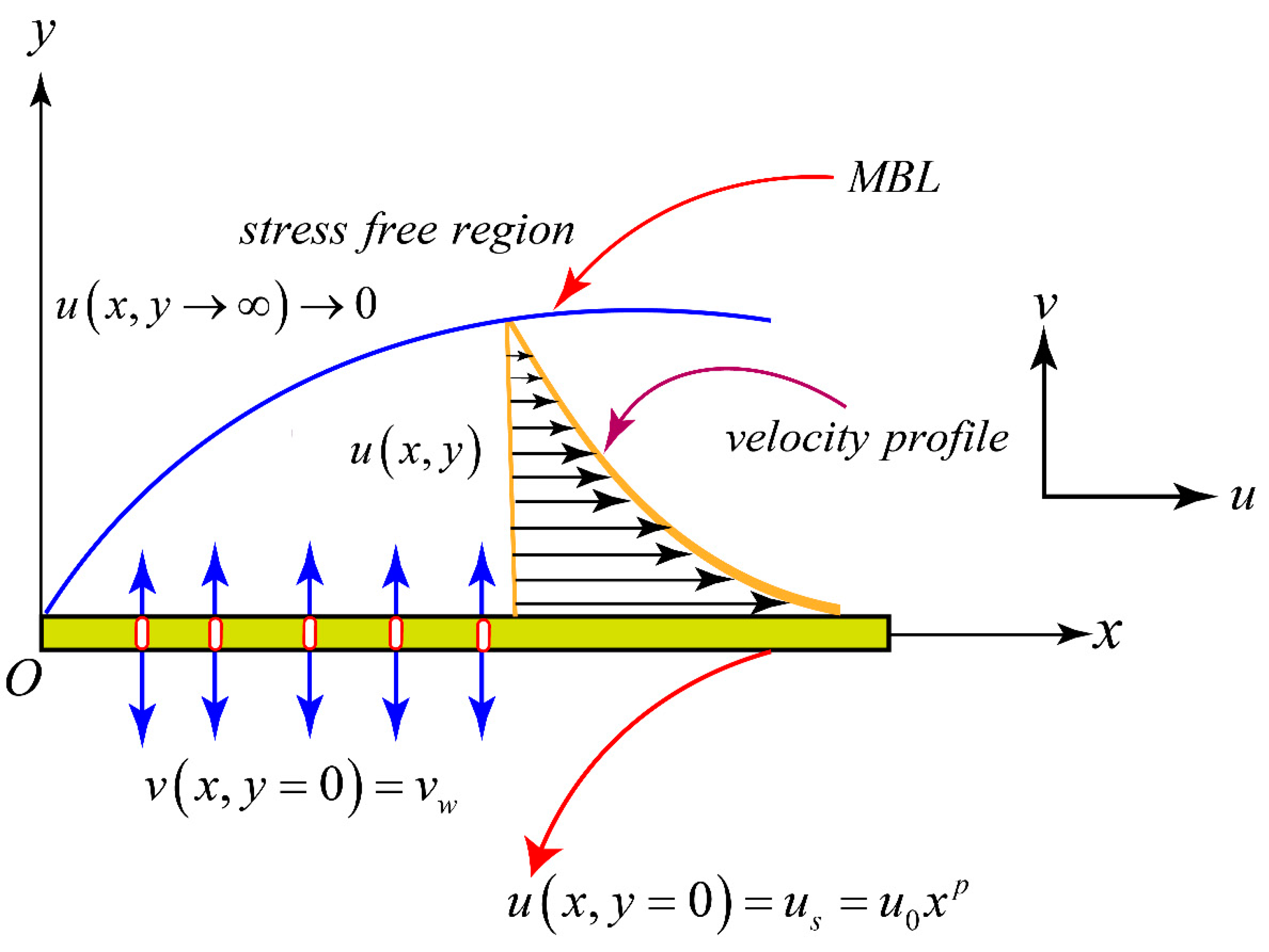
• The problem allows the similarity solution only when the transverse velocity at the boundary of the porous stretching surface is of the form $v_w\sim x^{\frac{p-1}{2}}.$
• The skin friction coefficient increases with enhancing the withdrawal parameter and decreases for the injection parameter.
• With an increasing injection, the one-equation model (local similarity method) overestimates the skin friction coefficient.
• For the increasing value of the velocity index parameter, the one-model approach, also known as the local similarity approach, underestimates the skin friction coefficient in the presence of suction.
• For increasing velocity index values, the one-model overestimates the skin friction coefficient in the presence of injection.
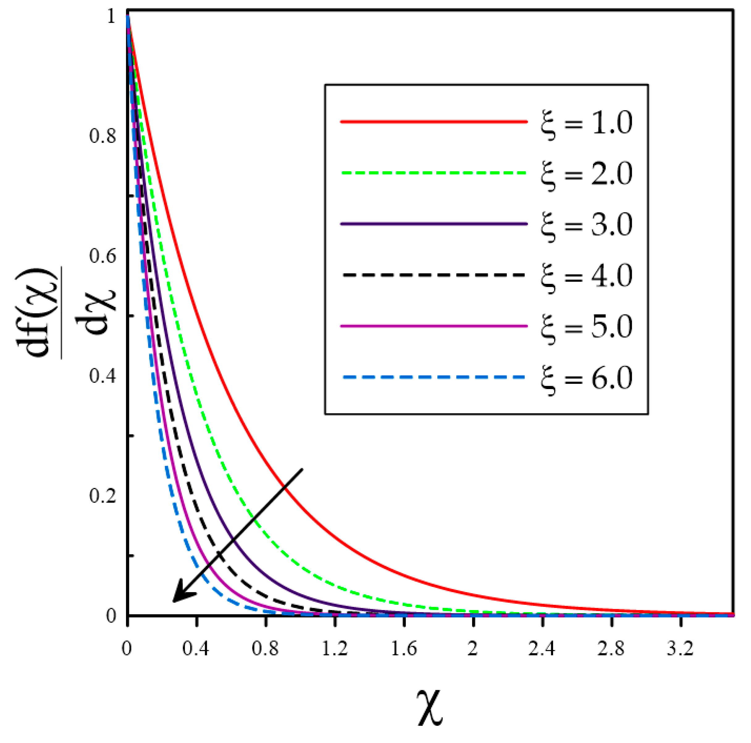
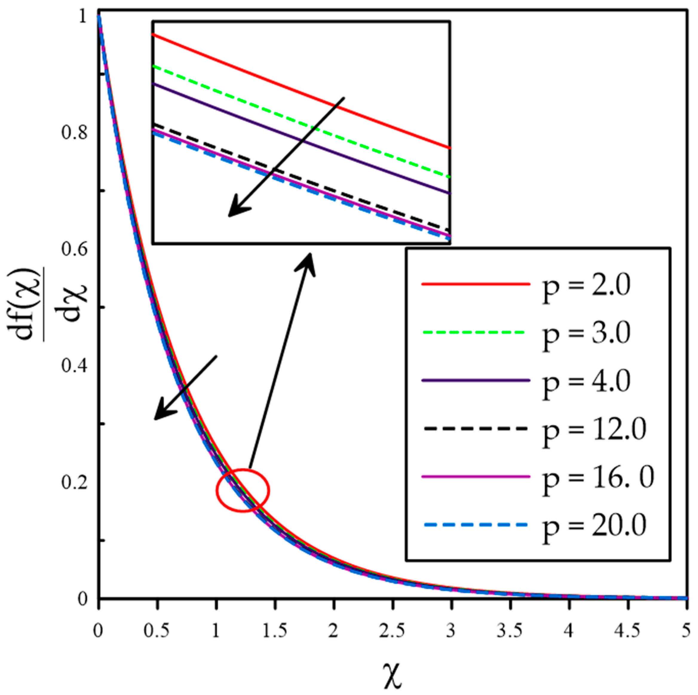
• The thickness of the non-similar boundary layer reduces with increasing suction and velocity index parameters.
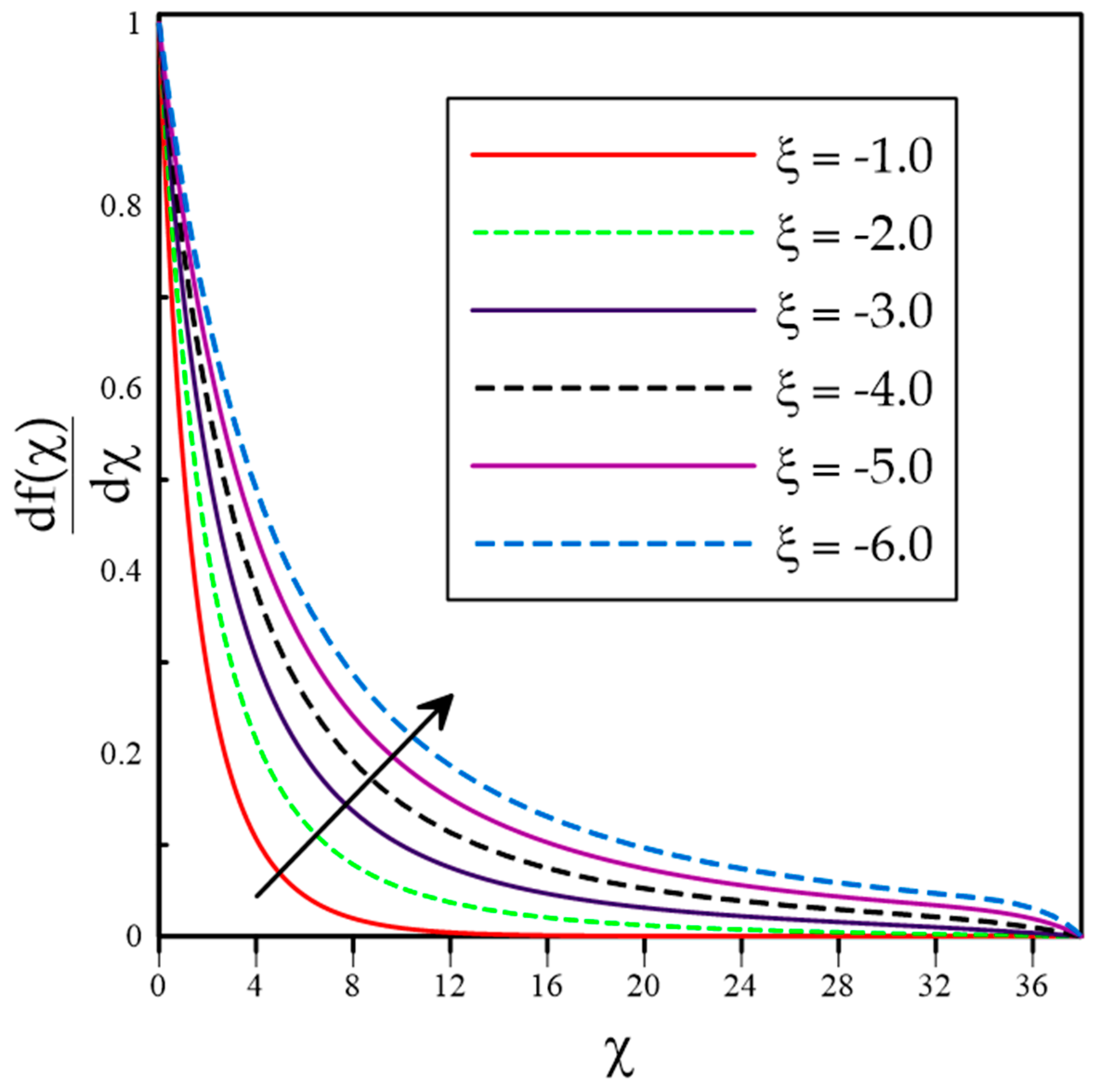
• The fluid inside the non-similar momentum boundary layer accelerates with increasing injection parameters.
• Future research may focus on thermal and second law analyses of fluid flow over a nonlinearly stretching surface with uniform lateral mass flux.

References

1. Erickson, L.E.; Fan, L.T.; Fox, V.G. Heat and mass transfer on a moving continuous flat plate with suction or injection. Ind. Eng. Chem. Fundam. 1966, 5, 19–25. [Google Scholar] [CrossRef]
2. Ishak, A.; Nazar, R.; Pop, I. Uniform suction/blowing effect on flow and heat transfer due to a stretching cylinder. Appl. Math. Model. 2008, 32, 2059–2066. [Google Scholar] [CrossRef]
3. Jha, B.K.; Isah, B.Y.; Uwanta, I.J. Combined effect of suction/injection on MHD free-convection flow in a vertical channel with thermal radiation. Ain Shams Eng. J. 2018, 9, 1069–1088. [Google Scholar] [CrossRef] [Green Version]
4. Yazdia, M.H.; Abdullah, S.; Hashim, I.; Sopian, K. Slip MHD liquid flow and heat transfer over non-linear permeable stretching surface with chemical reaction. Int. J. Heat Mass Transf. 2011, 54, 3214–3225. [Google Scholar] [CrossRef]
5. Crane, L.J. Flow past a stretching plate. ZAMP 1970, 21, 645–647. [Google Scholar] [CrossRef]
6. Makinde, O.D.; Aziz, A. Boundary layer flow of a nanofluid past a stretching sheet with a convective boundary condition. Int. J. Therm. Sci. 2011, 50, 1326–1332. [Google Scholar] [CrossRef]
7. Turkyilmazoglu, M. Analytic heat and mass transfer of the mixed hydrodynamic/thermal slip MHD viscous flow over a stretching sheet. Int. J. Mech. Sci. 2011, 53, 886–896. [Google Scholar] [CrossRef]
8. Qasim, M. Heat and mass transfer in a Jeffrey fluid over a stretching sheet with heat source/sink. Alex. Eng. J. 2013, 52, 571–575. [Google Scholar] [CrossRef] [Green Version]
9. Turkyilmazoglu, M.; Pop, I. Exact analytical solutions for the flow and heat transfer near the stagnation point on a stretching/shrinking sheet in a Jeffrey fluid. Int. J. Heat Mass Transf. 2013, 57, 82–88. [Google Scholar] [CrossRef]
10. Mehmood, A. Viscous Flows: Stretching and Shrinking of Surfaces; Springer: Berlin/Heidelberg, Germany, 2017. [Google Scholar]
11. Djebali, R.; Mebarek-Oudina, F.; Rajashekhar, C. Similarity solution analysis of dynamic and thermal boundary layers: Further formulation along a vertical flat plate. Phys. Scr. 2021, 96, 085206. [Google Scholar] [CrossRef]
12. Swain, K.; Mahanthesh, B.; Mebarek Oudina, F. Heat transport and stagnation-point flow of magnetized nanoliquid with variable thermal conductivity, Brownian moment, and thermophoresis aspects. Heat Transf. 2021, 50, 754–767. [Google Scholar] [CrossRef]
13. Gupta, P.S.; Gupta, A.S. Heat and mass transfer on a stretching sheet with suction or blowing. Can. J. Chem. Eng. 1977, 55, 744–746. [Google Scholar] [CrossRef]
14. Chen, C.K.; Char, M. Heat transfer of a continuous stretching surface with suction or blowing. J. Math. Anal. Appl. 1988, 135, 568–580. [Google Scholar] [CrossRef] [Green Version]
15. Naramgari, S.; Sulochana, C. MHD flow over a permeable stretching/shrinking sheet of a nanofluid with suction/injection. Alex. Eng. J. 2016, 55, 819–827. [Google Scholar] [CrossRef] [Green Version]
16. Megahed, A.M. Improvement of heat transfer mechanism through a Maxwell fluid flow over a stretching sheet embedded in a porous medium and convectively heated. Math. Comput. Simul. 2021, 187, 97–109. [Google Scholar] [CrossRef]
17. Kausar, M.S.; Hussanan, A.; Waqas, M.; Mamata, M. Boundary layer flow of micropolar nanofluid towards a permeable stretching sheet in the presence of porous medium with thermal radiation and viscous dissipation. Chin. J. Phys. 2022, 78, 435–452. [Google Scholar] [CrossRef]
18. Kumaran, V.; Banerjee, A.K.; Kumar, A.V.; Vajravelu, K. MHD flow past a stretching permeable sheet. Appl. Math. Comput. 2009, 210, 26–32. [Google Scholar] [CrossRef]
19. Mahanta, G.; Shaw, S. 3D Casson fluid flow past a porous linearly stretching sheet with convective boundary condition. Alex. Eng. J. 2015, 54, 653–659. [Google Scholar] [CrossRef]
20. Afridi, M.I.; Qasim, M.; Shafie, S. Entropy generation in hydromagnetic boundary flow under the effects of frictional and Joule heating: Exact solutions. Eur. Phys. J. Plus 2017, 132, 404. [Google Scholar] [CrossRef]
21. Pop, I.; Na, T.-Y. A note on MHD flow over a stretching permeable surface. Mech. Res. Commun. 1998, 25, 263–269. [Google Scholar] [CrossRef]
22. Khan, U.; Waini, I.; Ishak, A.; Pop, I. Unsteady hybrid nanofluid flow over a radially permeable shrinking/stretching surface. J. Mol. Liq. 2021, 331, 115752. [Google Scholar] [CrossRef]
23. Banks, W.H.H. Similarity Solutions of the Boundary Layer Equation for a Stretching Wall. J. De Mec. Theor. Et Appl. 1983, 2, 375–392. [Google Scholar]
24. Vajravelu, K. Viscous flow over a nonlinearly stretching sheet. Appl. Math. Comput. 2001, 124, 281–288. [Google Scholar] [CrossRef]
25. Ali, M.E. The Effect of Suction or Injection on the Laminar Boundary Layer Development Over a Stretched Surface. J. King Saud Univ. 1996, 8, 43–58. [Google Scholar] [CrossRef]
26. Jaafar, A.; Waini, I.; Jamaludin, A.; Nazar, R.; Pop, I. MHD flow and heat transfer of a hybrid nanofluid past a nonlinear surface stretching/shrinking with effects of thermal radiation and suction. Chin. J. Phys. 2022, 79, 13–27. [Google Scholar] [CrossRef]
27. Zaimi, K.; Ishak, A.; Pop, I. Boundary layer flow and heat transfer over a nonlinearly permeable stretching/shrinking sheet in a nanofluid. Sci. Rep. 2014, 4, 4404. [Google Scholar] [CrossRef] [Green Version]
28. Minkowycz, W.J.; Cheng, P. Local Non-similar solutions for free convective flow with uniform lateral mass flux in a porous medium. Lett. Heat Mass Transf. 1982, 9, 159–168. [Google Scholar] [CrossRef]
29. Afridi, M.I.; Chen, Z.; Qasim, M. Numerical Chebyshev finite difference examination of Lorentz force effect on a dissipative flow with variable thermal conductivity and magnetic heating: Entropy generation minimization. Z Angew. Math. Mech. 2022, e202200010. [Google Scholar] [CrossRef]
30. Hayat, T.; Qasim, M.; Abbas, Z. Homotopy solution for the unsteady three-dimensional MHD flow and mass transfer in a porous space. Commun. Nonlinear Sci. Numer. Simul. 2010, 15, 2375–2387. [Google Scholar] [CrossRef]
31. Koulali, A.; Abderrahmane, A.; Jamshed, W.; Hussain, S.M.; Nisar, K.S.; Abdel, A.; Yahia, I.S.; Eid, M.R. Comparative study on effects of thermal gradient direction on heat exchange between a pure fluid and a nanofluid: Employing finite volume method. Coatings 2021, 11, 12. [Google Scholar] [CrossRef]
32. Radouane, F.; Abderrahmane, A.; Oudina, F.M.; Ahmed, W.; Rashad, A.M.; Sahnoun, M.; Ali, H.M. Magneto-Free Convectiveof Hybrid Nanofluid inside Non-Darcy Porous Enclosure Containing an Adiabatic Rotating Cylinder. Energy Sour. Part A Recover. Util. Environ. Eff. 2020, 1–16. [Google Scholar] [CrossRef]
33. Shafiq, A.; Zari, I.; Rasool, G.; Tlili, I.; Khan, T.S. On the MHD Casson Axisymmetric Marangoni Forced Convective Flow of Nanofluids. Mathematics 2019, 7, 1087. [Google Scholar] [CrossRef] [Green Version]
34. Medebber, M.A.; Aissa, A.; Slimani ME, A.; Retiel, N. Numerical Study of Natural Convection in Vertical Cylindrical Annular Enclosure Filled with Cu-Water Nanofluid under Magnetic Fields. Defect Diffus. Forum 2020, 392, 123–137. [Google Scholar] [CrossRef]
35. Afridi, M.I.; Ashraf, M.U.; Qasim, M.; Wakif, A. Numerical simulation of entropy transport in the oscillating fluid flow with transpiration and internal fluid heating by GGDQM. Waves Random Complex Media 2022, 1–19. [Google Scholar] [CrossRef]
36. Shafiq, A.; Khan, I.; Rasool, G.; Sherif, E.M.; Sheikh, A.H. Influence of Single- and Multi-Wall Carbon Nanotubes on Magnetohydrodynamic Stagnation Point Nanofluid Flow over Variable Thicker Surface with Concave and Convex Effects. Mathematics 2020, 8, 104. [Google Scholar] [CrossRef] [Green Version]
37. Al-Kouz, W.; Medebber, M.A.; Elkot, M.A.; Abderrahmane, A.; Aimad, K.; Al-Farhany, K.; Jamshed, W.; Fldawig, H.M.; Saleel, C.A.; Nisar, K.S. Galerkin finite element analysis of Darcy—Brinkman—Forchheimer natural convective flow in conical annular enclosure with discrete heat sources. Energy Rep. 2021, 7, 6172–6181. [Google Scholar] [CrossRef]
38. Abderrahmane, A.; Qasem, N.A.A.; Younis, O.; Marzouki, R.; Mourad, A.; Shah, N.A.; Chung, J.D. MHD Hybrid Nanofluid Mixed Convection Heat Transfer and Entropy Generation in a 3-D Triangular Porous Cavity with Zigzag Wall and Rotating Cylinder. Mathematics 2022, 10, 769. [Google Scholar] [CrossRef]
39. Sparrow, E.M.; Quack, H.; Boerner, C.J. Local non-similarity boundary-layer solutions. Amercian Inst. Aeronaut. Astronaut. J. 1970, 8, 1936–1942. [Google Scholar] [CrossRef]
40. Sparrow, E.M.; Yu, H.S. Local non-similarity thermal boundary-layer solutions. ASME J. Heat Transf. Transf. 1978, 93, 328–334. [Google Scholar] [CrossRef]
41. Massoudi, M. Local non-similarity solutions for the flow of a non-Newtonian fluid over a wedge. Int. J. Non-Linear Mech. 2001, 36, 961–976. [Google Scholar] [CrossRef]
42. Liao, S.J. A general approach to get series solution of non-similarity boundary-layer flows. Commun. Nonlinear Sci. Numer. Simul. 2009, 14, 2144–2159. [Google Scholar] [CrossRef]
43. Liao, S.J. Homotopy Analysis Method in Nonlinear Differential Equations; Springer & Higher Education Press: Beijing, China, 2011; pp. 383–401. [Google Scholar]
44. Mureithi, E.W.; Mason, D.P. Local non-similarity solutions for a forced-free boundary layer flow with viscous dissipation. Math. Comput. Appl. 2010, 15, 558–573. [Google Scholar] [CrossRef]
45. Muhaimin, I.; Kandasamy, R. Local non-similarity solution for the impact of a chemical reaction in an MHD mixed convection heat and mass transfer flow over a porous wedge in the presence of suction/injection. J. Appl. Mech. Tech. Phys. 2010, 51, 721–731. [Google Scholar] [CrossRef]
46. Chamkha, A.J.; Rashad, M.; Golra, R.S.R. Non-Similar solutions for a mixed convection embedded in a porous medium saturated by a non-Newtonian nanofluid: Natural convection dominated regime. Int. J. Numer. Methods Heat Fluid Flow 2014, 24, 1471–1486. [Google Scholar] [CrossRef]
47. Farooq, U.; Hayat, T.; Alsaedi, A.; Liao, S.J. Series solutions of non-similarity boundary layer flows of nano-fluids over stretching surfaces. Numer. Algorithms 2015, 70, 43–59. [Google Scholar] [CrossRef]
48. Abdullah, A.; Ibrahim, F.S.; Chamkha, A.J. Non-similar solution of unsteady mixed convective flow near the stagnation point of a heated vertical plate in a porous medium saturated with a nano-fluid. J. Porous Media 2018, 21, 363–388. [Google Scholar] [CrossRef] [Green Version]
49. Afridi, M.I.; Qasim, M.; Khan, N.A.; Makinde, O.D. Minimization of entropy generation in MHD mixed convection flow with energy dissipation and Joule heating: Utilization of Sparrow-Quack-Boerner local non-similarity method. Defect Diffus. Forum 2018, 387, 63–77. [Google Scholar] [CrossRef]
50. Cui, J.; Razzaq, R.; Farooq, U.; Khan, W.A.; Farooq, F.B.; Muhammad, T. Impact of non-similar modeling for forced convection analysis of nano-fluid flow over stretching sheet with chemical reaction and heat generation. Alex. Eng. J. 2022, 61, 4253–4261. [Google Scholar] [CrossRef]
51. Kierzenka, J.; Shampine, L.F. A BVP Solver that Controls Residual and Error. J. Numer. Anal. Ind. Appl. Math. 2008, 3, 27–41. [Google Scholar]
52. Gilat, A.; Subramaniam, V. Numerical Methods for Engineers and Scientists an Introduction with Applications Using MATLAB; Wiley: Hoboken, NJ, USA, 2014. [Google Scholar]
Figure 1. Flow configuration with a coordinate system.
Mathematics 10 04159 g001
Figure 2. Velocity profile against the various values of withdrawal.
Mathematics 10 04159 g002
Figure 3. Velocity profile against the various values of injection parameter when p = 2.0 .
Mathematics 10 04159 g003
Figure 4. Velocity profile against the various values of velocity index parameter when ξ = 0.5 .
Mathematics 10 04159 g004