Deep 3D Volumetric Model Genesis for Efficient Screening of Lung Infection Using Chest CT Scans

Abstract

In the present outbreak of COVID-19, radiographic imaging modalities such as computed tomography (CT) scanners are commonly used for visual assessment of COVID-19 infection. However, personal assessment of CT images is a time-taking process and demands expert radiologists. Recent advancement in artificial intelligence field has achieved remarkable performance of computer-aided diagnosis (CAD) methods. Therefore, various deep learning-driven CAD solutions have been proposed for the automatic diagnosis of COVID-19 infection. However, most of them consider limited number of data samples to develop and validate their methods. In addition, various existing methods employ image-based models considering only spatial information in making a diagnostic decision in case of 3D volumetric data. To address these limitations, we propose a dilated shuffle sequential network (DSS-Net) that considers both spatial and 3D structural features in case of volumetric CT data and makes an effective diagnostic decision. To calculate the performance of the proposed DSS-Net, we combined three publicly accessible datasets that include large number of positive and negative data samples. Finally, our DSS-Net exhibits the average performance of 96.58%, 96.53%, 97.07%, 96.01%, and 98.54% in terms of accuracy, F1-score, average precision, average recall, and area under the curve, respectively, and outperforms various state-of-the-art methods.

1. Introduction

The unprecedented Coronavirus Disease 2019 (COVID-19) has affected millions of people worldwide by causing acute respiratory syndrome. According to a report by the World Health Organization on 30 May 2022, the number of COVID-19 cases surpassed 525 million, with a total death toll of more than 6.28 million worldwide. More-contagious variants of COVID-19 have mutated over time, further imperiling the world. Several types of vaccine have undergone clinical testing and have received US Food and Drug Administration clearance. However, early and effective diagnostic measures are still preferable to overcome the burden on healthcare systems in developing countries. Currently, the reverse transcription-polymerase chain reaction (RT-PCR) test is used as an efficient measure for diagnosing COVID-19-positive cases. Nevertheless, it can only discriminate between COVID-19 positive and negative cases without providing additional information related to the severity of this deadly virus. In this regard, radiographic imaging modalities, such as computed tomography (CT), are used to assess the severity of this deadly virus by capturing a visual representation of the lung. However, personal evaluation of lung CT scans is still a time-consuming process that requires professional radiologists.

The recent era of artificial intelligence (AI) has gained remarkable success in developing efficient computer-aided diagnosis (CAD) tools in the medical field [1,2,3]. In general, these CAD methods are used to analyze the generated data of different imaging modalities by applying efficient AI algorithms and make an accurate diagnostic decision similar to that of a medical expert. Recently, a new class of AI methods, known as “deep learning” (DL) algorithms, has achieved remarkable success owing to the breakthrough performance of these algorithms in imaging data analysis [1,2,3,4,5,6,7]. In the medical domain, such DL methods can mimic the diagnostic capability of medical experts through a training process using medical imaging data and then make an accurate diagnostic decision. In the context of 2D/3D imaging data, convolutional neural networks (CNNs) are a variety of DL algorithm that has garnered significant attention. In the literature [1,2,3,4,5,6,7,8,9,10,11,12,13,14,15], various CNN models have been devised for the diagnostic assessment of COVID-19 patients using chest radiographs, such as CT scans and X-rays. These models are configured for a diagnostic application using an annotated training dataset and finally tested with independent testing datasets.

Fang et al. [4] assessed the results of RT-PCR tests and chest CT scan data of 51 patients. The efficiency of chest CT analysis compared with RT-PCR at an early stage was 98% versus 71%, with p < 0.001 [4]. Subsequently, several CAD solutions have evolved utilizing the strength of DL-driven classification and segmentation models for the effective diagnosis of COVID-19 [1,2,3,4,5,6,7,8,9,10,11,12,13,14,15]. Oh et al. [6] introduced a patch-based deep feature extraction scheme intended to exploit infected and normal lesion patterns using a limited number of chest X-ray scans. The overall pipeline includes a lung segmentation model that extracts lung lobes from a given X-ray image. Then, a patched-based classification model makes a final diagnostic decision. Similarly, Singh et al. [7] proposed a multi-objective differential evolution approach to obtain an optimally trained DL model using a limited number of chest CT scan data. The ultimate goal of their method was to classify positive and negative cases based on CT data analysis. Subsequently, Castiglione et al. [1] proposed an optimized DL model to differentiate infected and noninfected patients into binary classes by scanning lung CT scan data. Similarly, Zhang et al. [2] proposed an advanced residual-learning-based diagnostic framework to differentiate positive COVID-19 patients from heterogeneous lung data.

In the context of data synthesis, Lan et al. [3] proposed a novel hierarchical polishing spline algorithm for the reconstruction of synthesized CT data of COVID-19 patients. Synthesized data can be used to achieve a more accurate assessment of COVID-19 severity. Jiang et al. [8] further applied a conditional generative adversarial network (C-GAN) for data synthesis and a U-Net model for the segmentation of pulmonary manifestations of COVID-19 in chest CT scans. Similarly, Zhang et al. [9] proposed a novel version of C-GAN to synthesize high-quality CT images. The experimental results with 2D and 3D U-Net attained considerable segmentation performance compared with their method using synthetic data. Furthermore, Fan et al. [10] introduced a semisupervised learning approach for efficiently training their proposed segmentation network, Inf-Net, with unlabeled data.

Recently, the strength of ensemble CNN models has been investigated in the context of automatic diagnosis of COVID-19. For example, Lan et al. [11] proposed an ensemble DL model for the effective identification of COVID-19-positive patients using chest X-ray images based on COVID-Net. Similarly, Kundu et al. [12] performed a COVID-19 recognition task using lung CT data with a fuzzy integral-based ensemble design by integrating four pretrained CNN models. Rajaraman et al. [13] proposed an iteratively pruned ensemble model for the detection of pulmonary manifestations of COVID-19 in chest X-ray scans. Various individual pretrained deep models were tested, and the best-performing models were combined using different ensemble strategies to improve the overall diagnostic performance. Saha et al. [14] developed an ensemble classifier for the successful diagnosis of COVID-19 using X-ray data by combining the prediction scores of different machine learning classifiers.

For the accurate identification of COVID-19-associated lesion sites in chest radiography images, semantic segmentation models are used instead of deep classification networks. For example, El-Bana et al. [15] proposed a deep-learning-based multitask framework that includes a classification-followed segmentation stage to detect and segment specific types of infection manifestations in CT images. Later, Zheng et al. [16] addressed a similar multiclass segmentation problem and proposed a multiscale discriminative network (MSD-Net) that can detect infected regions of varied sizes. The experimental findings show better MSD-Net efficiency compared with other baseline models. Similarly, Chen et al. [17] proposed an effective 3D deep-CNN framework for the segmentation of COVID-19-associated lesion regions in COVID-19 CT images. A patch-based technique was implemented to ensure the applicability of the 3D-CNN model and eliminate unnecessary background information. Furthermore, the adoption of a 3D attention model enhanced the attention capability of the model for infected regions.

Although significant diagnostic outcomes have been achieved in various studies [18,19,20,21,22,23,24,25,26,27,28,29,30], the proposed DL models might be subject to overfitting/underfitting and generalization problems owing to the limited dataset sizes. In addition, various methods make a slice-based diagnostic decision using selective slices of the entire CT volume, which also requires time and manual effort to select appropriate CT slices for effective diagnosis. Existing 3D CNN-based methods require an input CT volume of a fixed length. There has been limited research related to 3D CNN-based CAD solutions that explored both spatial and 3D structural features from an input CT volume of variable length and make class predictions. In 2D classification models, the loss of 3D structural information may result in false predictions and diminish the overall prediction probability of the testing data.

To address the limitations of existing studies, a deep sequence-based diagnostic and retrieval framework is proposed for the efficient screening of COVID-19-positive cases using the entire CT volume of variable length. The quantitative results demonstrate the superior performance of the proposed CAD framework compared with various state-of-the-art methods. The distinct contributions of this study are as follows:

-

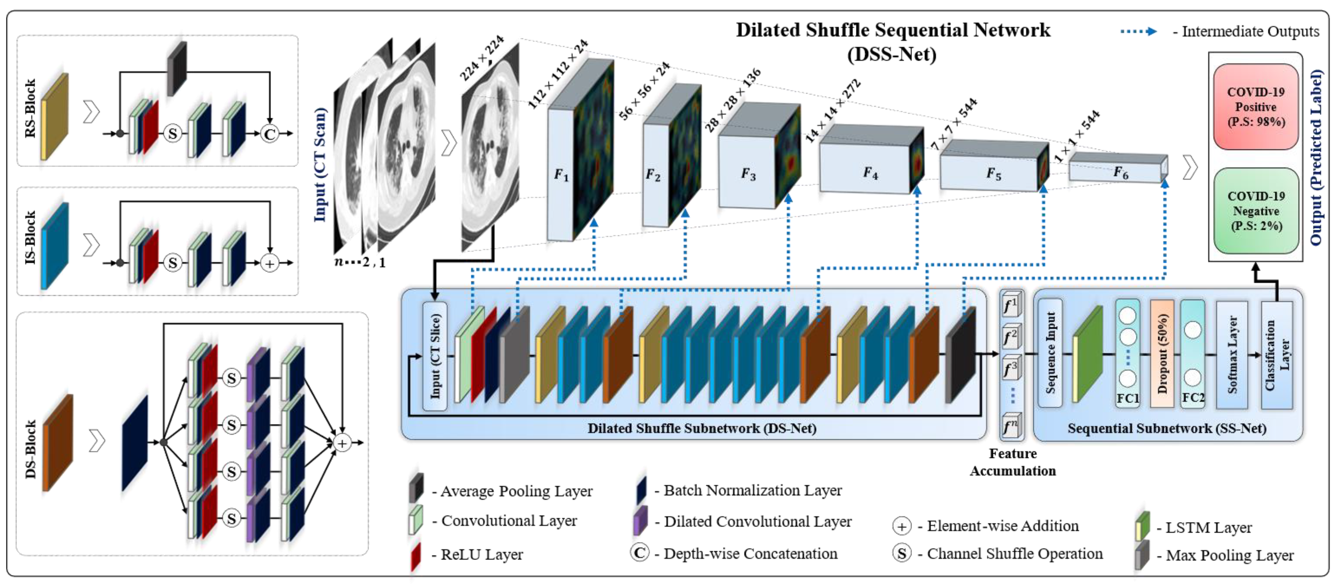
A sequence-based 3D model called the “dilated shuffle sequential network” (DSS-Net) is proposed for the automatic and robust diagnosis of COVID-19 using a chest CT volume of variable length.

-

A dilated shuffle block (DS-Block) is proposed that is based on multiscale dilated convolution and shuffle operation to explore multiscale contextual features from the input CT volume, which ultimately resulted in improved performance. In addition, all convolutional layers in the proposed model take advantage of the grouped convolution operation to achieve lightweight (1.57 million parameters) characteristics in the context of volumetric data analysis without causing performance degradation.

-

The network design uses an input CT volume of variable length rather than employing a fixed-length sequence, and it leverages transfer learning in volumetric data analysis without influencing the overall training parameters.

-

The proposed DSS-Net is available to the public on request for research and education.

The rest of this article is ordered as follows. In Section 2, the overall proposed framework is described with an emphasis on the network design, structure, and workflow. In Section 3, the datasets, experimental setup, and quantitative results are described. In Section 4, a brief discussion with a final conclusion is presented.

2. Proposed Method

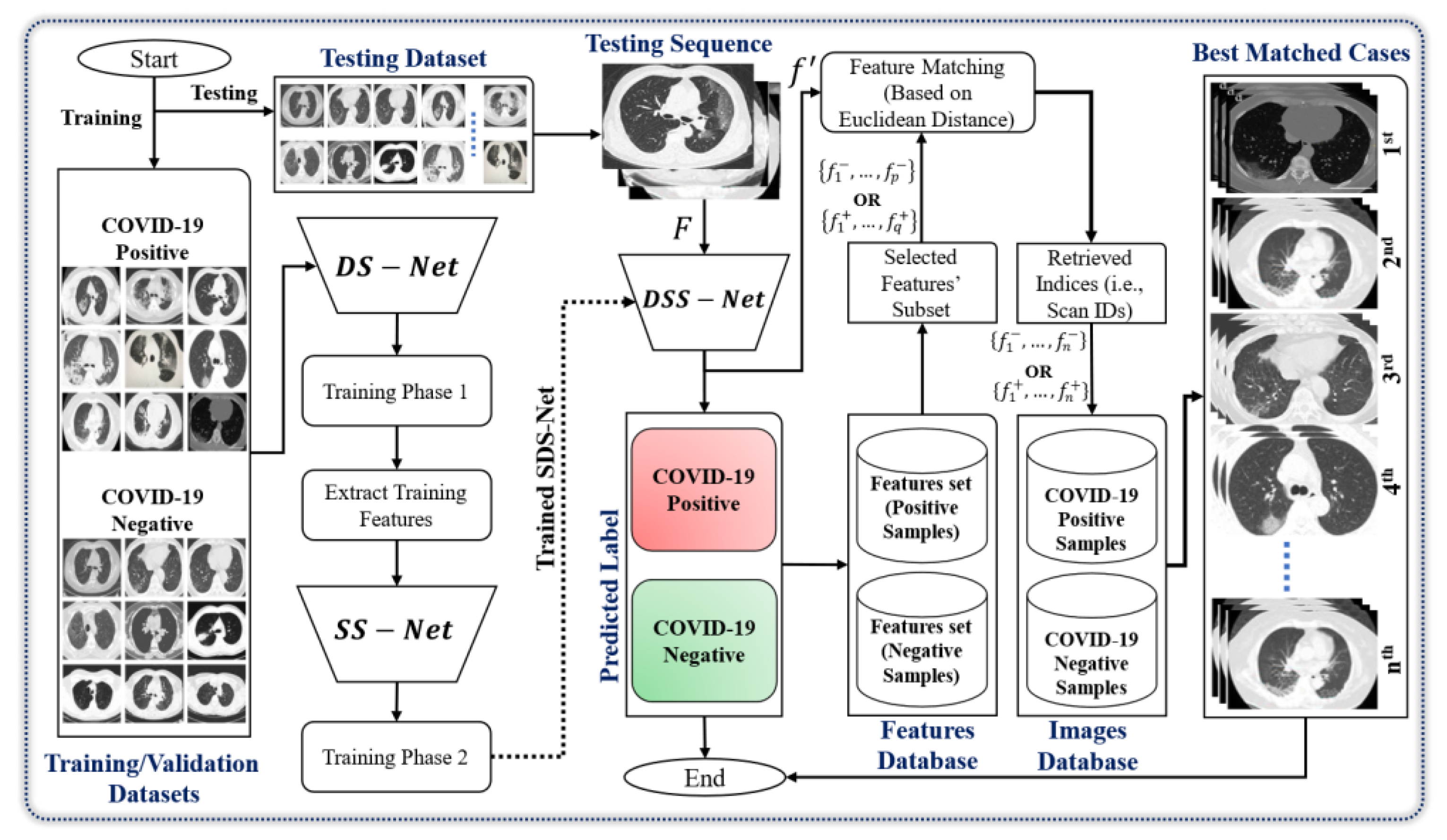
2.1. Workflow Overview

The purpose of this study was to develop a deep-classification-driven retrieval framework for the automatic diagnosis of COVID-19 using a variable-length chest CT scan of $n$ successive slices (i.e., ${\mathit{F}}^1,{\mathit{F}}^2,{\mathit{F}}^3,\dots ,{\mathit{F}}^n)$. A simplified workflow of the proposed scheme is shown in Figure 1. The entire framework comprises a deep classification model (DSS-Net) followed by the retrieval phase to accomplish the diagnostic assessment and then retrieve the relevant cases. In the first phase, DSS-Net was trained sequentially to exploit multiscale spatial and 3D structural features from an independent training dataset. Consequently, the trained DSS-Net makes a diagnostic evaluation for the given volumetric CT data by predicting its class label (COVID-19 positive or negative). In the second phase of classification-driven retrieval, the best-matched relevant instances (CT slices) related to the input sample are retrieved. These best-matched retrieval results can further help radiologists in the subjective evaluation of computer diagnostic decisions and eventually result in an effective diagnostic decision.

2.2. Dilated Shuffle Sequential Network Structure

The proposed DSS-Net is based on two subnetworks: dilated shuffle subnetwork (DS-Net) and sequential subnetwork (SS-Net). They utilize the strengths of (1) the proposed dilated shuffle (DS) block (Figure 2) based on multiscale dilated convolution layers, (2) two existing shuffle blocks, residual shuffle (RS)-block and identity shuffle (IS)-block in Figure 2, and (3) a revised variant of the recurrent neural network (RNN), the long short-term memory (LSTM) model.

(A) Dilated Shuffle Subnetwork: The complete structure of the first subnetwork includes three DS blocks, three RS blocks, 10 IS blocks, and some other layers, as shown in Figure 2. The proposed DS block mainly utilizes the strength of multiscale dilated convolution and channel shuffle operations in a mutually advantageous manner to achieve the superior performance of the final DSS-Net. In general, existing shuffle blocks (RS and IS blocks) are based on grouped convolutional layers and are designed to reduce the computational cost without causing performance degradation. The addition of skip connections further avoids the vanishing gradient problem in the training process and achieves the optimal convergence of the entire network. Therefore, the strength of these shuffle blocks was utilized to develop the DS block. Conventional shuffle blocks consist of three grouped convolutional layers, a channel shuffle operation, and a residual connection, as shown in the bottom-left corner of Figure 2. Mathematically, the input tensor ${\mathit{F}}_i\in {\mathcal{R}}^{w_i\times h_i\times d_i}$ is processed using the following layer-wise transformations after passing through these shuffle blocks.

$${\Psi }_{RS}\left({\mathit{F}}_i\right)=h_{{\mathit{\phi }}_3}\left(h_{{\mathit{\phi }}_2}\left(S\left(h_{{\mathit{\phi }}_1}\left({\mathit{F}}_i\right)\right)\right)\right)\odot A\left({\mathit{F}}_i\right)$$

(1)

$${\Psi }_{IS}\left({\mathit{F}}_i\right)=h_{{\phi }_3}\left(h_{{\phi }_2}\left(S\left(h_{{\phi }_1}\left({\mathit{F}}_i\right)\right)\right)\right)+{\mathit{F}}_i$$

(2)

where ${\Psi }_{RS}\left(·\right)$ and ${\Psi }_{IS}\left(·\right)$ denote the RS and IS blocks, respectively, as transfer functions. Here, $h_{{\mathit{\phi }}_1}\left(·\right)$, $h_{{\mathit{\phi }}_2}\left(·\right)$, and $h_{{\mathit{\phi }}_3}\left(·\right)$ represent the grouped convolutional layers with training parameters ${\mathit{\phi }}_1$, ${\mathit{\phi }}_2$, and ${\mathit{\phi }}_3$, respectively. The notations $S\left(·\right)$ and $A\left(·\right)$ represent channel shuffling and average pooling operations, respectively. The symbols $\odot$ and $+$ represent the depth-wise feature concatenation and pointwise addition operations, respectively.

The RS block consists of a residual connection based on a 3 × 3 average pooling layer, denoted as $A\left(·\right)$ in Equation (1), which mainly downsamples the input tensor ${\mathit{F}}_i\in {\mathcal{R}}^{w_i\times h_i\times d_i}$ by a factor of two. The IS-block consists of an identity residual connection that incorporates the input tensor ${\mathit{F}}_i$ as residual information without influencing its dimension. The structure of the proposed DS-block comprises four parallel-connected dilated convolutional layers (with dilation rates of 1, 3, 5, and 7), four shuffle operations, eight grouped convolutional layers, and an identity residual connection. Mathematically, input tensor ${\mathit{F}}_i\in {\mathcal{R}}^{w_i\times h_i\times d_i}$ undergoes the following transformations after passing through a DS block.

$${\Psi }_{DS}\left({\mathit{F}}_i\right)={{\displaystyle \sum }}_{r=1,3,5,7}{h}_{{\phi }_3}\left(h_{{\phi }_2^r}^{\ast }\left(S\left(h_{{\phi }_1}\left({\mathit{F}}_i\right)\right)\right)\right)+{\mathit{F}}_i$$

(3)

where ${\Psi }_{DF}\left(·\right)$ denotes the DS block as the transfer function. Here, $h_{{\mathit{\phi }}_2^r}^{\ast }\left(·\right)$ represents dilated convolutional layers with a dilation rate $r$. The key insight behind the development of DS block is to incorporate additional multiscale contextual features from the output of each IS block, which ultimately results in better performance. A quantitative ablation study (see Section 3) showed the significant strength of the DS block in implementing our final DSS-Net.

(B) Sequential Subnetwork: SS-Net includes a revised variant of RNNs (the LSTM model), which resolves the vanishing gradient problem in the training process. In general, the structure of LSTM models is based on the cascaded connectivity of multiple LSTM cells. Each cell includes a memory cell unit and three gate units (input, forget, and output gates) [5]. LSTM models are appropriate for fixed- and variable-length moving sequences of 2D CT slices and are designed to exploit temporal dependencies among successive images. In addition, a cascade of 2D-CNN and LSTM models can leverage transfer learning for volumetric data analysis without influencing the overall training parameters. Therefore, the strength of LSTM was exploited to design the lightweight SS-Net for the effective classification of volumetric CT data in the medical domain.

2.3. Dilated Shuffle Sequential Network Workflow

Figure 2 and

Table 1. Layer-wise configuration details of the proposed dilated shuffle sequential network (DSS-Net) (“Conv: Convolutional layer”, “N: Number of nodes in FC layer”, “R: Dilation rate”, “Itr.: Number of iterations”).

Layer Name	Input Size	Filter Size	Filter Depth(R)	Str.	Itr.	Output Size
Input	224 × 224	–	–	–	1	–
Conv	224 × 224 × 3	3 × 3	24	2	1	112 × 112 × 24
Max-pooling	112 × 112 × 24	3 × 3	1	2	1	56 × 56 × 24
RS block	56 × 56 × 24	1 × 1, 3 × 3, 1 × 1 3 × 3	112, 112, 112 1	1, 2, 1 2	1	28 × 28 × 136
IS block	28 × 28 × 136	1 × 1, 3 × 3, 1 × 1	136, 136, 136	1, 1, 1	2	28 × 28 × 136
DS block	28 × 28 × 136	1 × 1, 3 × 3, 1 × 1 1 × 1, 3 × 3, 1 × 1 1 × 1, 3 × 3, 1 × 1 1 × 1, 3 × 3, 1 × 1	136, 136, 136(1) 136, 136, 136(3) 136, 136, 136(5) 136, 136, 136(7)	1, 1, 1 1, 1, 1 1, 1, 1 1, 1, 1	1	28 × 28 × 136
RS block	28 × 28 × 136	1 × 1, 3 × 3, 1 × 1 3 × 3	136, 136, 136 1	1, 2, 1 2	1	14 × 14 × 272
IS block	14 × 14 × 272	1 × 1, 3 × 3, 1 × 1	272, 272, 272	1, 1, 1	6	14 × 14 × 272
DS block	14 × 14 × 272	1 × 1, 3 × 3, 1 × 1 1 × 1, 3 × 3, 1 × 1 1 × 1, 3 × 3, 1 × 1 1 × 1, 3 × 3, 1 × 1	272, 272, 272(1) 272, 272, 272(3) 272, 272, 272(5) 272, 272, 272(7)	1, 1, 1 1, 1, 1 1, 1, 1 1, 1, 1	1	14 × 14 × 272
RS block	14 × 14 × 272	1 × 1, 3 × 3, 1 × 1 3 × 3	272, 272, 272 1	1, 2, 1 2	1	7 × 7 × 544
IS block	7 × 7 × 544	1 × 1, 3 × 3, 1 × 1	544, 544, 544	1, 1, 1	2	7 × 7 × 544
DS block	7 × 7 × 544	1 × 1, 3 × 3, 1 × 1 1 × 1, 3 × 3, 1 × 1 1 × 1, 3 × 3, 1 × 1 1 × 1, 3 × 3, 1 × 1	544, 544, 544(1) 544, 544, 544(3) 544, 544, 544(5) 544, 544, 544(7)	1, 1, 1 1, 1, 1 1, 1, 1 1, 1, 1	1	7 × 7 × 544
Avg-pooling	7 × 7 × 544	7 × 7	1	1	1	1 × 1 × 544
Sequence Input	1 × 1 × 544 × n	–	–	–	1	–
LSTM	1 × 1 × 544 × n	–	–	–	1	1 × 1 × 600
FC1	1 × 1 × 600	–	128N			1 × 1 × 128
Dropout (50%)	1 × 1 × 128	–	–	–	1	1 × 1 × 128
FC2	1 × 1 × 128	–	2N	–	1	1 × 1 × 2
Softmax	1 × 1 × 2	–	–	–	1	1 × 1 × 2
Classification	1 × 1 × 2	–	–	–	1	2

present the complete workflow and layer-wise configuration of our proposed DSS-Net, respectively. First, a 3 × 3 convolutional layer extracts low-level semantic information from each CT slice $\mathit{F}$ and produces an output feature map of size 112 × 112 × 24, which is further downsampled by a 3 × 3 max-pooling layer into a new output tensor of size 56 × 56 × 24. Afterward, a stack of 16 shuffle blocks (including a total of three DS blocks, three RS blocks, 10 IS blocks, and some other layers, as shown in Figure 2) successively exploits the multilevel semantic information from the output tensor of the previous block and eventually generates a high-level feature map of size 7 × 7 × 544. Ultimately, the last 7 × 7 average-pooling layer downsampled this high-level feature map and created a final output feature vector of size 1 × 1 × 544. Consequently, a multiscale semantic representation of the input slice $\mathit{F}$ was obtained as an output feature vector $\mathit{f}$ of size 1 × 1 × 544.

In the case of $n$ successive CT slices (i.e., ${\mathit{F}}^1,{\mathit{F}}^2,{\mathit{F}}^3,\dots ,{\mathit{F}}^n),$the proposed DSS-Net successively processes each input slice and outputs a set of $n$ feature vectors (i.e., ${\mathit{f}}^1,{\mathit{f}}^2,{\mathit{f}}^3,\dots ,{\mathit{f}}^n)$ of size 1 × 1 × 544 × n. All these feature vectors are accumulated and then further processed by the second-stage SS-Net (Figure 2) to exploit 3D structural features and perform class prediction. First, a sequence input layer of SS-Net passes the accumulated set of $n$ feature vectors (${\mathit{f}}^1,{\mathit{f}}^2,{\mathit{f}}^3,\dots ,{\mathit{f}}^n)$ to the LSTM layer, which exploits 3D structural dependencies among these feature vectors, and finally generates a single feature vector ${\mathit{h}}_n$ of size 1 × 1 × 600. Successively, the first fully connected layer (FC1; Figure 2 and Table 1) further exploits more discriminative patterns from ${\mathit{h}}_n$ by mapping them into a 1 × 1 × 128 low-dimensional feature vector. Furthermore, a dropout layer (having a dropout factor of 0.5) was included after FC1 to avoid overfitting. Finally, a stack of three additional layers: (1) FC2, (2) softmax, and (3) classification layers, predicts a single class label for the entire CT scan. The FC2 layer identifies the larger hidden patterns in the output of the preceding dropout layer, and the softmax layer (including the softmax function as ${\mathit{f}}_i^{\prime }=e^{{\mathit{f}}_i}/{{\displaystyle \sum }}_{i=1}^2{e}^{{\mathit{f}}_i}$ [5]) further transforms the output of the FC2 layer in terms of probability. Finally, the classification layer performs class prediction and assigns a class label to the input CT scan based on the highest probability score.

2.4. Training Loss

A two-step training process was performed sequentially to attain the optimal convergence of the final DSS-Net. In the first step, the first DS-Net was trained to exploit and learn the spatial features from the entire training dataset, denoted as ${\langle \left[{\mathit{F}}_T\right]}_{i=1}^p,{\left[l_T\right]}_{i=1}^p\rangle$, using a cross-entropy (CE) loss function [17]. The initial weights of different shuffle blocks (in DS-Net) were obtained from a pretrained S-Net trained with a large-scale ImageNet dataset [26] using the CE loss function. Therefore, a similar loss was applied to train the DS-Net model. In the next step, all training data samples ${\left[{\mathit{F}}_T\right]}_{i=1}^p$ were converted into feature vectors ${\left[{\mathit{f}}_T\right]}_{i=1}^p$ after processing each data sample using the trained DS-Net model. Consequently, a new training dataset (${\langle \left[{\mathit{f}}_T\right]}_{i=1}^p,{\left[l_T\right]}_{i=1}^p\rangle$) was obtained in the feature domain. In the second stage, SS-Net was trained to learn the 3D structural dependencies from the feature-level data samples ${\langle \left[{\mathit{f}}_T\right]}_{i=1}^p,{\left[l_T\right]}_{i=1}^p\rangle$ using the same CE loss function. The overall two-step loss of the proposed DSS-Net can be expressed as

$${\mathcal{L}}_{DSS-Net}=\left\{\begin{array}{c}\underset{w_{DS-Net}^{\prime }}{arg min} {\mathcal{L}}_1\left({\psi }_{w_{DS-Net}}({\left[{\mathit{F}}_T\right]}_{i=1}^p\right),{\left[l_T\right]}_{i=1}^p) \\ \underset{w_{SS-Net}^{\prime }}{arg min} {\mathcal{L}}_2\left({\psi }_{w_{SS-Net}}({\left[{\mathit{f}}_T\right]}_{i=1}^p\right),{\left[l_T\right]}_{i=1}^p) \end{array} \right.$$

(4)

where ${\psi }_1$ and ${\psi }_2$ represent DS-Net and SS-Net, respectively, as the transfer functions. Here, ${\mathcal{L}}_1\left(·\right)$ and ${\mathcal{L}}_2\left(·\right)$ denote CE loss functions. After training, the performance of the final DSS-Net was assessed using an independent testing dataset, denoted as ${\langle \left[{\mathit{F}}_{Ts}\right]}_{i=1}^r,{\left[l_{Ts}\right]}_{i=1}^r\rangle$.

3. Results and Analysis

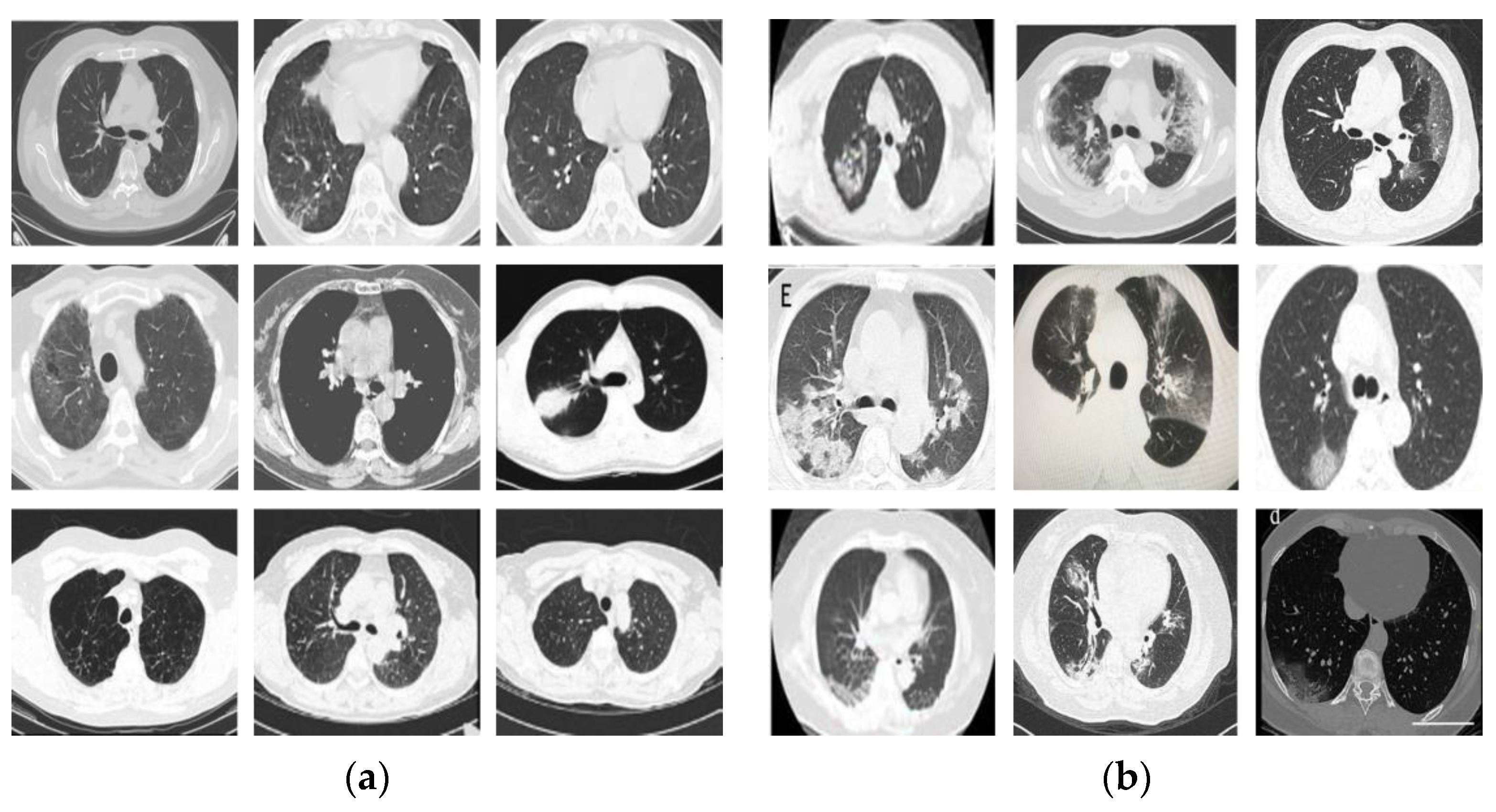
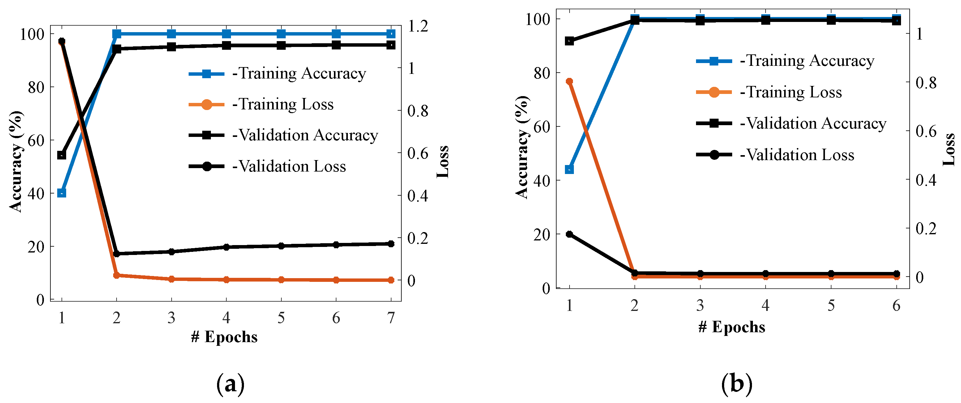
3.1. Dataset and Experimental Setup

To analyze the proposed method quantitatively, three publicly available chest CT datasets selected in a previous study [29] were combined to create a single large-scale database that includes 5471 data samples of 2789 different patients. The entire dataset was subdivided into COVID-19 negative and positive categories according to the ground-truth labels of the data. The negative data collection comprised 2217 data samples from 1129 patients. The positive data collection included 3254 data samples collected from 1660 patients. Figure 3 depicts a few representative CT scans from the chosen dataset to demonstrate the visual difference between COVID-19 negative and positive instances. All the simulations were executed in a MATLAB (R2019a) framework (with the deep-learning toolbox) using a desktop PC with the following specifications: (1) Intel Core i7 processor, (2) 16-GB RAM, (3) NVIDIA GeForce GPU (GTX 1070), and (4) Windows 10 operating system. A stochastic gradient descent optimizer with a learning rate of 0.001 was utilized in the optimization strategy to train both subnetworks. Mini-batch sizes of 10 and 100 were selected for training DS-Net and SS-Net, respectively. All other hyperparameters were initialized using the default parametric setting of the deep-learning toolbox provided by MATLAB (R2019a). In all the experiments, five-fold cross validation was accomplished using 70% (3830 data samples), 10% (547 data samples), and 20% (1094 data samples) of the whole data for model training, validation, and testing, respectively. For fair analysis, different patient data were used for training, validation, and testing.

Previous methods lack validation datasets, which may result in underfitting or overfitting problems. To prevent these problems, an independent validation dataset (10% of the total dataset) was included, and a training stop criterion was defined that stops the training process after the validation accuracy converges, as explained in Algorithm 1. Figure 4 shows the training/validation losses and accuracies of both subnetworks. In Figure 4, the convergence of the training and validation curves (with respect to losses and accuracies) validates that neither model was overfitted with the training dataset. Finally, the quantitative testing results of our proposed and other methods were assessed in terms of average accuracy (ACC), F1-score (F1), average recall (AR), average precision (AP), and area under the curve (AUC).

Algorithm 1: Two-step training stop algorithm.
Input: trainable parameters, $w_{DS-Net}$,$w_{SS-Net}$; learning-rate, $\eta$; maximum number of epochs, $N$; $p$ training samples denoted as $\langle {\left[{\mathit{F}}_T\right]}_{i=1}^p,{\left[l_T\right]}_{i=1}^p\rangle$; and $q$ validation samples denoted as $\langle {\left[{\mathit{F}}_V\right]}_{i=1}^q,{\left[l_V\right]}_{i=1}^q\rangle$
1	Initialize trainable parameters$w_{DS-Net}$ (Pretrained weights of [26] for shuffle blocks and Gaussian random weights for remaining blocks/layers), $w_{SS-Net}$ (Gaussian random weights)
2	/* Step 1: Continue the training of the first DS-Net */
3	for$n=1,2,3,\dots ,N$do
4	get: ${\left[l_T^{\prime }\right]}_{i=1}^p={\psi }_{w_{DS-Net}}\left({\left[{\mathit{F}}_T\right]}_{i=1}^p\right)$, ${\left[l_V^{\prime }\right]}_{i=1}^q={\psi }_{DS}\left({\left[{\mathit{F}}_V\right]}_{i=1}^q\right)$
5	update: $w_{DS-Net}=w_{DS-Net}-\eta .\nabla {\mathcal{L}}_1\left({\left[l_T^{\prime }\right]}_{i=1}^p,{\left[l_T\right]}_{i=1}^p\right)$
6	check: if $accuracy\left({\left[l_V^{\prime }\right]}_{i=1}^q,{\left[l_V\right]}_{i=1}^q\right)$ converges do stop the training end
7	End
8	Output 1: Learned weights $w_{DS-Net}^{\prime }$ for DS-Net
9	/* Step 2: Extract features dataset from the avg-pooling layer of DS-Net */
10	get: ${\left[{\mathit{f}}_T\right]}_{i=1}^p={\mathsf{{\rm Y}}}_{Avg-pool}\left({\psi }_{DS-Net},{\left[{\mathit{F}}_T\right]}_{i=1}^p\right)$, ${\left[{\mathit{f}}_V\right]}_{i=1}^q={\mathsf{{\rm Y}}}_{Avg-pool}\left({\psi }_{DS-Net},{\left[{\mathit{F}}_V\right]}_{i=1}^q\right)$
11	Output 2: Training and validation feature dataset:${\left[{\mathit{f}}_T\right]}_{i=1}^p$, ${\left[{\mathit{f}}_V\right]}_{i=1}^q$
12	/* Step 3: Continue the training of SS-Net */
13	for$n=1,2,3,\dots ,N$do
14	get: ${\left[l_T^{\prime }\right]}_{i=1}^p={\psi }_{w_{SS-Net}}\left({\left[{\mathit{f}}_T\right]}_{i=1}^p\right)$, ${\left[l_V^{\prime }\right]}_{i=1}^q={\psi }_{w_{SS-Net}}\left({\left[{\mathit{f}}_V\right]}_{i=1}^q\right)$
15	update:$w_{SS-Net}=w_{SS-Net}-\eta .\nabla {\mathcal{L}}_2\left({\left[l_T^{\prime }\right]}_{i=1}^p,{\left[l_T\right]}_{i=1}^p\right)$
16	check: if $accuracy\left({\left[l_V^{\prime }\right]}_{i=1}^q,{\left[l_V\right]}_{i=1}^q\right)$ converges do stop training end
17	end
18	Output 3: Learned weights $w_{SS-Net}^{\prime }$ for S-Net

3.2. Testing Results (Ablation Studies)

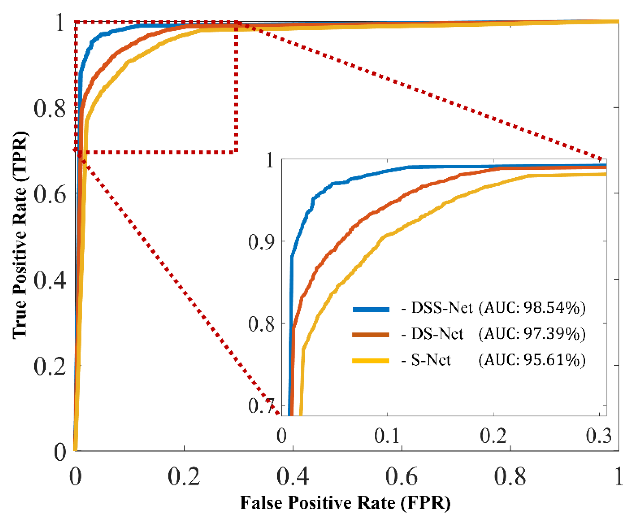
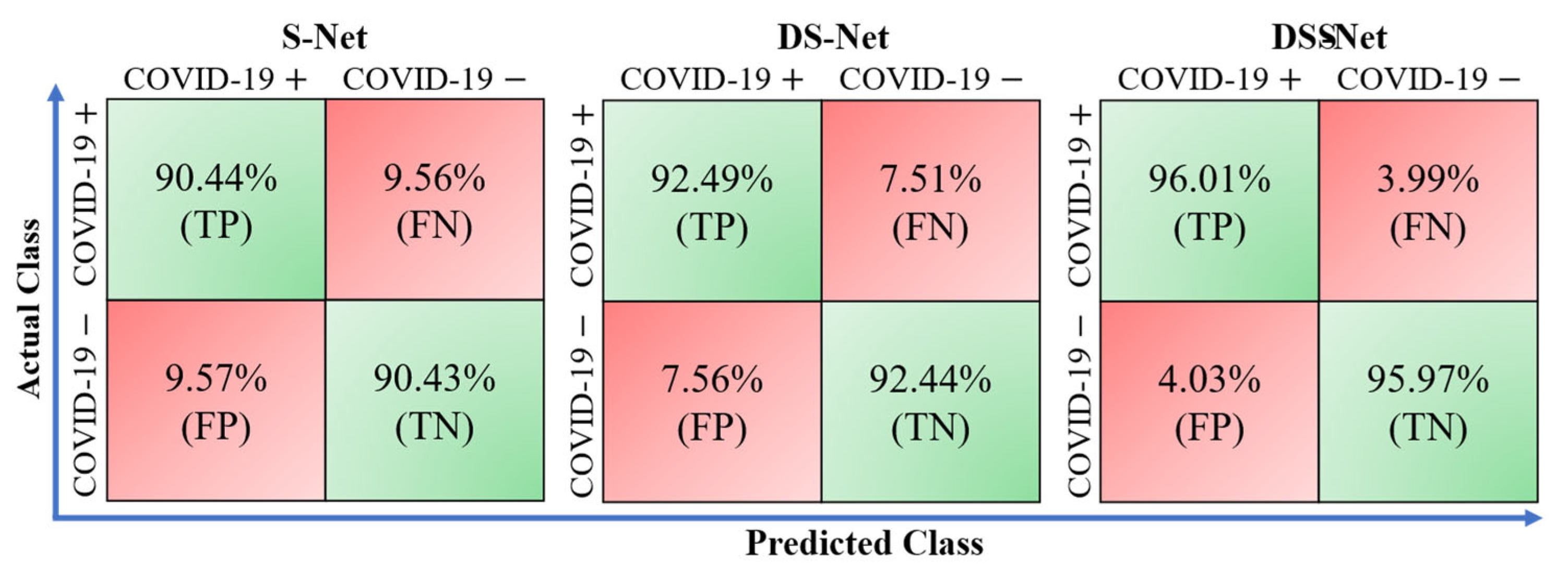
DSS-Net exploits spatial and 3D structural features from a given volumetric CT scan and makes a diagnostic decision (i.e., either COVID-19 negative or positive). A five-fold quantitative assessment of DSS-Net is summarized in

Table 2. Quantitative performance comparison of DSS-Net, DS-Net, and S-Net. The average results are highlighted in boldface. (“#: The number of”, “Avg.: Average”, “Std: Standard deviation”, “unit: %”).

Model	#Fold	ACC	F1	AP	AR	AUC
Shuffle Network (S-Net) [26]	1	96.07	96.02	95.63	96.4	99.46
	2	92.69	92.41	93.03	91.8	97.94
	3	89.76	89.49	90.94	88.08	94.72
	4	97.63	97.54	97.6	97.47	99.71
	5	82.1	82.16	86.23	78.47	86.23
	Avg. (Std)	91.65 (6.15)	91.52 (6.10)	92.69 (4.41)	90.44 (7.68)	95.61 (5.61)
Dilated Shuffle Subnetwork (DS-Net)	1	95.79	95.66	95.5	95.81	98.64
	2	94.33	94.16	94.89	93.44	98.54
	3	89.95	89.62	90.82	88.45	96.22
	4	96.07	95.92	96.04	95.8	99.11
	5	90.41	90.13	91.36	88.93	94.43
	Avg. (Std)	93.31 (2.94)	93.1 (3.02)	93.72 (2.44)	92.49 (3.60)	97.39 (2.00)
Dilated Shuffle Sequential Network (DSS-Net)	1	99.36	99.34	99.25	99.43	99.99
	2	97.17	97.06	97.18	96.93	99.59
	3	94.88	94.77	95.65	93.9	98.24
	4	98.81	98.77	98.72	98.82	99.75
	5	92.69	92.73	94.53	90.99	95.14
	Avg (Std)	96.58 (2.79)	96.53 (2.77)	97.07 (2.00)	96.01 (3.54)	98.54 (2.02)

. The comparative results of DS-Net (proposed second-best) and S-Net (baseline model) are also presented in Table 2. These comparative results show the contribution of multiscale feature aggregation using DS blocks and second-stage SS-Net in terms of quantitative gains. In particular, DS-Net (comprising DS, RS, and IS blocks) surpasses S-Net (comprising only RS and IS blocks) with average gains of 1.66%, 1.58%, 1.03%, 2.05%, and 1.78% in terms of ACC, F1, AP, AR, and AUC, respectively. Subsequently, the addition of SS-Net (in DSS-Net) improved the performance of the first-stage DS-Net, with average gains of 3.27%, 3.43%, 3.35%, 3.52%, and 1.15% in terms of ACC, F1, AP, AR, and AUC, respectively. DSS-Net significantly outperformed S-Net (baseline model), with average gains of 4.93%, 5.01%, 4.38%, 5.57%, and 2.93% in terms of ACC, F1, AP, AR, and AUC, respectively. In a t-test analysis, DSS-Net accomplished an average p-value of 0.0014 $\left(p<0.01\right)$ and 0.0003 $\left(p<0.01\right)$ compared with DS-Net and S-Net, respectively. The lower p-values $(p<0.01)$ imply that DSS-Net significantly outperformed them with a 99% confidence score.

The receiver operator characteristic (ROC) response of DSS-Net compared with DS-Net and S-Net is further highlighted in Figure 5. Each curve (Figure 5) presents a trade-off between the average false-positive rate (FPR) and true-positive rate (TPR) of a model according to different thresholds varying from 0 to 1 in 0.01 increments. The best validation performance was achieved for each method at a particular classification threshold. The optimal threshold values for DSS-Net (best model), DS-Net (second-best model), and S-Net (baseline model) were 0.513, 0.514, and 0.507, respectively. Compared with S-Net, DSS-Net considerably decreased the FPR from 9.57% to 4.03% with an average gain of 5.54% and improved the TPR from 90.44% to 96.01% with an average gain of 5.57%, as shown in Figure 6. In addition, DS-Net also decreased the FPR from 9.57% to 7.56% with an average gain of 2.01% and improved the TPR from 90.44% to 92.49% with an average gain of 2.05% compared with S-Net, as shown in Figure 6.

The initial trainable parameters of the shuffle blocks in DS-Net were acquired from a pretrained S-Net through transfer learning. Therefore, DS-Net and DSS-Net were trained from scratch to highlight the quantitative gain of transfer learning in the proposed method. The comparative results of transfer learning and training from scratch are presented in

Table 3. Comparative results of the proposed DSS-Net and DS-Net with and without performing transfer learning. (“T.L: Transfer learning”).

Model	T.L	ACC (Std)	F1 (Std)	AP (Std)	AR (Std)	AUC (Std)
Dilated Shuffle Subnetwork (DS-Net)	✕	83.44 (11.11)	82.78 (11.53)	84.82 (9.6)	80.96 (13.31)	86.79 (12.53)
	✓	93.31 (2.94)	93.1 (3.02)	93.72 (2.44)	92.49 (3.60)	97.39 (2.00)
Dilated Shuffle Sequential Network (DSS-Net)	✕	88.61 (12.91)	89.06 (12.21)	92.44 (7.36)	86.35 (16.17)	87.69 (16.51)
	✓	96.58 (2.79)	96.53 (2.77)	97.07 (2.00)	96.01 (3.54)	98.54 (2.02)

. In the case of DS-Net, the results imply (Table 3) that transfer learning outperforms training from scratch with average gains of 9.87%, 10.32%, 8.9%, 11.53%, and 10.6% in terms of ACC, F1, AP, AR, and AUC, respectively. Similarly, significant performance gains of 7.97%, 7.47%, 4.63%, 9.66%, and 10.85% were observed in terms of ACC, F1, PRE, REC, and AUC, respectively, for DSS-Net.

3.3. Comparison

Different CAD techniques have been proposed for the automated diagnostic screening of COVID-19. Here, a comparative performance analysis is presented of DSS-Net with different state-of-the-art CAD methods related to COVID-19 diagnostics [18,19,20,21,22,23,24,25,26,27,28,29,30]. However, most previous solutions consider a limited number of datasets. For a fair comparison, the findings of these current approaches [18,19,20,21,22,23,24,25,26,27,28,29,30] were compared with the datasets selected in this study using the same experimental setting as the method. The quantitative results of DSS-Net and various baseline approaches [18,19,20,21,22,23,24,25,26,27,28,29,30] are presented in

Table 4. Comparative performance analysis of DSS-Net with various state-of-the-art methods. (“#: The number of”).

Study	#Par. (M)	ACC	F1	AP	AR	AUC
Brunese et al. [18]	134.27	89.66	89.54	91.43	87.81	92.35
Farooq et al. [19]	23.54	90.30	90.22	92.17	88.53	92.79
Minaee et al. [20]	1.24	89.84	89.48	89.91	89.06	93.86
Khan et al. [21]	139.58	91.54	91.33	92.26	90.47	94.54
Alsharman et al. [22]	5.98	89.73	89.53	90.4	88.73	94.91
Misra et al. [23]	11.18	92.96	92.76	93.41	92.14	95.06
Hu et al. [24]	0.86	91.65	91.52	92.69	90.44	95.61
Ardakani et al. [25]	42.56	90.30	90.26	92.17	88.64	95.71
Apostolopoulos et al. [26]	2.24	92.95	92.85	93.81	91.94	96.51
Martínez et al. [27]	4.27	93.68	93.49	94.19	92.82	96.67
Jaiswal et al. [28]	18.11	94.17	94.03	94.63	93.46	97.36
Owais et al. [29]	3.16	94.72	94.60	95.22	94.00	97.50
Tsiknakis et al. [30]	21.81	94.57	94.41	94.89	93.94	97.93
Proposed	1.57	96.58	96.53	97.07	96.01	98.54

. DSS-Net exceeds all the baseline models in terms of quantitative performance (Table 4) and is ranked as the best model. In addition, the method of Tsiknakis et al. [30] ranked second among all other methods [18,19,20,21,22,23,24,25,26,27,28,29]. Nevertheless, DSS-Net outperformed that model [30] with average gains of 2.01%, 2.12%, 2.18%, 2.07%, and 0.61% in terms of ACC, F1, AP, AR, and AUC, respectively. In a t-test analysis, DSS-Net outperformed the method of Tsiknakis et al. [30] at a 99% confidence score by reaching an average p-value of 0.0019 $(p<0.01)$. In addition, the number of learnable parameters of DSS-Net is approximately 13.89 times lower than that in the previous model [30] (i.e., proposed DSS-Net: 1.57 million << Tsiknakis et al. [30]: 21.81 million). Consequently, the proposed model stands out among all the baseline techniques [18,19,20,21,22,23,24,25,26,27,28,29,30] because of its improved performance and lower number of parameters.

In a further related study, Hu et al. [24] applied an existing pretrained network for automatic diagnosis of COVID-19, which includes approximately 0.71 million fewer trainable parameters than those of the proposed DSS-Net (i.e., our proposed DSS-Net: 1.57 million > Hu et al. [24]: 0.86 million). Nevertheless, the quantitative results of DSS-Net are significantly higher than those of a previously proposed method [24], with average gains of 4.93%, 5.01%, 4.38%, 5.57%, and 2.93% in terms of ACC, F1, AP, AR, and AUC, respectively. Moreover, in a t-test analysis, DSS-Net outperformed the previous method [24] at a 99% confidence score by reaching an average p-value of 0.0003 $(p<0.01)$. In another study, the method of Minaee et al. [20] also contains approximately 0.33 million fewer parameters than the proposed DSS-Net (i.e., proposed DSS-Net: 1.57 million > Minaee et al. [20]: 1.24 million). However, the quantitative results of DSS-Net were significantly higher than those of a previous method [20], with average gains of 6.74%, 7.05%, 7.16%, 6.95%, and 4.68% in terms of ACC, F1, AP, AR, and AUC, respectively. A t-test analysis also revealed superior performance at a 99% confidence score, with an average p-value of 0.0001 $(p<0.01)$.

In conclusion, one can infer the following interpretations from this comparative analysis. The method of Tsiknakis et al. [30] shows quantitative results comparable to those of the proposed method. However, the computational cost (in terms of the number of training parameters) of the previous method [30] is significantly higher (approximately 13.89 times) than that of the methods in this study. Second, the method proposed by Hu et al. [24] includes a 50% lower number of trainable parameters than that of the proposed model. However, its quantitative performance is significantly lower than that of DSS-Net. In addition, despite the lower number of training parameters in a previous report [20], the quantitative performance gain of DSS-Net is significantly higher than that reported by Minaee et al. [20].

4. Discussion and Conclusions

In general, 2D-CNNs explore only spatial features from each input slice of given volumetric data and make a diagnostic decision. However, 3D-CNNs explore given volumetric data in 2D and 3D directions, exploring spatial and 3D structural features, and make a class prediction. In the first scenario, 2D-CNNs disregard 3D structural features, which can cause performance deficiencies. In the second scenario, 3D-CNNs comprise millions of trainable parameters and require high computational power for training. To address these problems, a 3D classification model was proposed for the precise classification of volumetric data. The proposed network design leverages transfer learning in volumetric data analysis without influencing the overall training parameters. It can also be used to classify variable-length sequences. Network design mainly leverages multiscale contextual features (DS blocks) to achieve state-of-the-art performance. DS-Net extracts a set of $n$ multiscale spatial feature vectors from given volumetric CT data. The second-stage SS-Net then exploits 3D structural features from a set of $n$ spatial feature vectors and makes the final diagnostic decision (i.e., COVID-19 negative or positive).

In the second stage, classification-driven content retrieval was performed, and the most-relevant instances (CT slices) were retrieved for the provided CT data as an additional output. Figure 7 presents the qualitative classification and retrieval results of our proposed framework. The results in Figure 7 show the predicted class label, prediction score, and best-matched data sample corresponding to each input CT scan. Five best-matched data samples were retrieved from the testing database corresponding to each input data sample (Figure 1). Specifically, a set of negative (${\mathit{F}}^{-}=\left\{{\mathit{f}}_1^{-},{\mathit{f}}_2^{-}, \dots ,{\mathit{f}}_p^{-}\right\}$) or positive (${\mathit{F}}^{+}=\left\{{\mathit{f}}_1^{+},{\mathit{f}}_2^{+},\dots ,{\mathit{f}}_q^{+}\right\}$) feature vectors was chosen from the feature database based on the predicted class label (Figure 1). Here, $p$ and $q$ are the numbers of negative and positive cases, respectively. All these feature vectors (${\mathit{F}}^{-}$ and ${\mathit{F}}^{+}$) were extracted from the training dataset that includes both COVID-19 negative and positive data samples and stored as a feature database (Figure 1). Subsequently, a Euclidean-distance-based matching algorithm was employed to select a subset of $n$ best-matched features (in this case, $n=5$) from the selected set of feature vectors corresponding to the query feature vector ${\mathit{f}}^{\prime }$ (extracted from the testing data sample). Finally, the selected subset of $n$ best-matched features was used to retrieve the corresponding CT slices from the testing database, as shown in Figure 7. Such retrieved cases can further assist medical experts in validating CAD decisions subjectively.

Figure 8 shows a few samples of misclassified testing cases together with their predicted scores. The existence of identical lesion shapes in COVID-19 negative and positive datasets may cause these incorrect predictions (false-negative and false-positive cases). Furthermore, inadequate data annotation might lead to incorrect predictions. However, medical specialists can reduce these inaccuracies by visually assessing the projected outputs (i.e., prediction score and best-matched retrieved cases). Despite the substantial performance of the proposed diagnostic framework, there are drawbacks to the proposed CAD approach that might affect its overall efficacy in a clinical context. The main concern is the issue of generalizability, especially in cases that show a small ratio of infected lung. Second, real-world data can show high intraclass variance because of several types of CT imaging modalities and may affect the diagnostic results. However, these constraints can be resolved by incorporating a large repository of well-annotated datasets as training/validation data. In future work, it is planned to investigate more-diversified datasets and resolve generalizability concerns thoroughly.

References

1. Castiglione, A.; Vijayakumar, P.; Nappi, M.; Sadiq, S.; Umer, M. COVID-19: Automatic detection of the novel coronavirus disease from CT images using an optimized convolutional neural network. IEEE Trans. Ind. Inform. 2021, 17, 6480–6488. [Google Scholar] [CrossRef]
2. Zhang, M.; Chu, R.; Dong, C.; Wei, J.; Lu, W.; Xiong, N. Residual learning diagnosis detection: An advanced residual learning diagnosis detection system for COVID-19 in industrial internet of things. IEEE Trans. Ind. Inform. 2021, 17, 6510–6518. [Google Scholar] [CrossRef]
3. Lan, T.; Cai, Z.; Ye, B. A novel spline algorithm applied to COVID-19 computed tomography image reconstruction. IEEE Trans. Ind. Inform. 2022, 18, 7804–7813. [Google Scholar] [CrossRef]
4. Fang, Y.; Zhang, H.; Xie, J.; Lin, M.; Ying, L.; Pang, P.; Ji, W. Sensitivity of chest CT for COVID-19: Comparison to RTPCR. Radiology 2020, 296, 200432. [Google Scholar] [CrossRef]
5. Heaton, J. Artificial Intelligence for Humans; Heaton Research, Inc.: Scotts Valley, CA, USA, 2013. [Google Scholar]
6. Oh, Y.; Park, S.; Ye, J.C. Deep learning COVID-19 features on CXR using limited training data sets. IEEE Trans Med. Imaging 2020, 39, 2688–2700. [Google Scholar] [CrossRef]
7. Singh, D.; Kumar, V.; Kaur, M. Classification of COVID-19 patients from chest CT images using multi-objective differential evolution–based convolutional neural networks. Eur. J. Clin. Microbiol. Infect. Dis. 2020, 39, 1379–1389. [Google Scholar] [CrossRef]
8. Jiang, Y.; Chen, H.; Loew, M.H.; Ko, H. COVID-19 CT image synthesis with a conditional generative adversarial network. IEEE J. Biomed. Health Inform. 2021, 25, 441–452. [Google Scholar] [CrossRef]
9. Zhang, P.; Zhong, Y.; Deng, Y.; Tang, X.; Li, X. CoSinGAN: Learning COVID-19 infection segmentation from a single radiological image. Diagnostics 2020, 10, 901. [Google Scholar] [CrossRef]
10. Fan, D.P.; Zhou, T.; Ji, G.-P.; Zhou, Y.; Chen, G.; Fu, H.; Shen, J.; Shao, L. Inf-net: Automatic COVID-19 lung infection segmentation from CT images. IEEE Trans. Med. Imaging 2020, 39, 2626–2637. [Google Scholar] [CrossRef] [PubMed]
11. Tang, S.; Wang, C.; Nie, J.; Kumar, N.; Zhang, Y.; Xiong, Z.; Barnawi, A. EDL-COVID: Ensemble deep learning for COVID-19 case detection from chest x-ray images. IEEE Trans. Ind. Inform. 2021, 17, 6539–6549. [Google Scholar] [CrossRef]
12. Kundu, R.; Singh, P.K.; Mirjalili, S.; Sarkar, R. COVID-19 detection from lung CT-Scans using a fuzzy integral-based CNN ensemble. Comput. Biol. Med. 2021, 138, 104895. [Google Scholar] [CrossRef] [PubMed]
13. Rajaraman, S.; Siegelman, J.; Alderson, P.O.; Folio, L.S.; Folio, L.R.; Antani, S.K. Iteratively pruned deep learning ensembles for COVID-19 detection in chest X-rays. IEEE Access 2020, 8, 115041–115050. [Google Scholar] [CrossRef]
14. Saha, P.; Sadi, M.S.; Islam, M.M. EMCNet: Automated COVID-19 diagnosis from X-ray images using convolutional neural network and ensemble of machine learning classifiers. Inform. Med. Unlocked 2021, 22, 100505. [Google Scholar] [CrossRef]
15. El-bana, S.; Al-Kabbany, A.; Sharkas, M. A multi-task pipeline with specialized streams for classification and segmentation of infection manifestations in COVID-19 scans. PeerJ Comput. Sci. 2020, 6, e303. [Google Scholar] [CrossRef]
16. Zheng, B.; Liu, Y.; Zhu, Y.; Yu, F.; Jiang, T.; Yang, D.; Xu, T. MSD-Net: Multi-scale discriminative network for COVID-19 lung infection segmentation on CT. IEEE Access 2020, 8, 185786–185795. [Google Scholar] [CrossRef] [PubMed]
17. Chen, C.; Zhou, K.; Zha, M.; Qu, X.; Guo, X.; Chen, H.; Wang, Z.; Xiao, R. An effective deep neural network for lung lesions segmentation from COVID-19 CT images. IEEE Trans. Ind. Inform. 2021, 17, 6528–6538. [Google Scholar] [CrossRef]
18. Brunese, L.; Mercaldo, F.; Reginelli, A.; Santone, A. Explainable deep learning for pulmonary disease and coronavirus COVID-19 detection from X-rays. Comput. Meth. Programs Biomed. 2020, 196, 105608. [Google Scholar] [CrossRef] [PubMed]
19. Farooq, M.; Hafeez, A. COVID-ResNet: A deep learning framework for screening of COVID19 from radiographs. arXiv 2020, arXiv:2003.14395. [Google Scholar] [CrossRef]
20. Minaee, S.; Kafieh, R.; Sonka, M.; Yazdani, S.; Soufi, G.J. Deep-COVID: Predicting COVID-19 from chest X-ray images using deep transfer learning. Med. Image Anal. 2020, 65, 101794. [Google Scholar] [CrossRef]
21. Khan, I.U.; Aslam, N. A deep-learning-based framework for automated diagnosis of COVID-19 using X-ray images. Information 2020, 11, 419. [Google Scholar] [CrossRef]
22. Alsharman, N.; Jawarneh, I. GoogleNet CNN neural network towards chest CT-coronavirus medical image classification. J. Comput. Sci. 2020, 16, 620–625. [Google Scholar] [CrossRef]
23. Misra, S.; Kafieh, R.; Sonka, M.; Yazdani, S.; Soufi, G.J. Multi-channel transfer learning of chest X-ray images for screening of COVID-19. Electronics 2020, 9, 1388. [Google Scholar] [CrossRef]
24. Hu, R.; Ruan, G.; Xiang, S.; Huang, M.; Liang, Q.; Li, J. Automated diagnosis of COVID-19 using deep learning and data augmentation on chest CT. medRxiv 2020. [Google Scholar] [CrossRef]
25. Ardakani, A.A.; Kanafi, A.R.; Acharya, U.R.; Khadem, N.; Mohammadi, A. Application of deep learning technique to manage COVID-19 in routine clinical practice using CT images: Results of 10 convolutional neural networks. Comput. Biol. Med. 2020, 121, 103795. [Google Scholar] [CrossRef] [PubMed]
26. Apostolopoulos, I.D.; Mpesiana, T.A. COVID-19: Automatic detection from X-ray images utilizing transfer learning with convolutional neural networks. Australas. Phys. Eng. Sci. Med. 2020, 43, 635–640. [Google Scholar] [CrossRef] [Green Version]
27. Martínez, F.; Martínez, F.; Jacinto, E. Performance evaluation of the NASNet convolutional network in the automatic identification of COVID19. Int. J. Adv. Sci. Eng. Inf. Techn. 2020, 10, 662–667, 662. [Google Scholar] [CrossRef]
28. Jaiswal, A.; Gianchandani, N.; Singh, D.; Kumar, V.; Kaur, M. Classification of the COVID-19 infected patients using densenet201 based deep transfer learning. J. Biomol. Struct. Dyn. 2021, 39, 5682–5689. [Google Scholar] [CrossRef]
29. Owais, M.; Yoon, H.S.; Mahmood, T.; Haider, A.; Sultan, H.; Park, K.R. Light-weighted ensemble network with multilevel activation visualization for robust diagnosis of COVID19 pneumonia from large-scale chest radiographic database. Appl. Soft Comput. 2021, 108, 107490. [Google Scholar] [CrossRef] [PubMed]
30. Tsiknakis, N.; Trivizakis, E.; Vassalou, E.E.; Papadakis, G.Z.; Spandidos, D.A.; Tsatsakis, A.; Sánchez-García, J.; López-González, R.; Papanikolaou, N.; Karantanas, A.H.; et al. Interpretable artificial intelligence framework for COVID-19 screening on chest X-rays. Exp. Ther. Med. 2020, 20, 727–735. [Google Scholar] [CrossRef]
Figure 1. Schematic workflow of the proposed diagnostic framework contains the following three parts: (a) data preprocessing, (b) model development and validation using training and testing data, and (c) finally retrieving the best-matched cases from the previous record.
Mathematics 10 04160 g001
Figure 2. Overall architecture of the proposed dilated shuffle sequential network (DSS-Net) comprising two subnetworks: dilated shuffle subnetwork (DS-Net) and sequential subnetwork (SS-Net).
Mathematics 10 04160 g002
Figure 3. Visual illustration of a few example chest CT slices of COVID-19 (a) negative and (b) positive cases. The positive data samples mainly include consolidation, bilateral, ground-glass opacity, and pleural effusion.
Mathematics 10 04160 g003
Figure 4. Training/validation accuracies and losses of the proposed (a) DS-Net and (b) DSS-Net.
Mathematics 10 04160 g004
Figure 5. Comparative ROC plots of DSS-Net (best model), DS-Net (second-best model), and S-Net (baseline model). These plots show the trade-off between the average false-positive rate (FPR) and true-positive rate (TPR) of each model according to different thresholds.
Mathematics 10 04160 g005
Figure 6. Performance comparison of DSS-Net, DS-Net, and S-Net in terms of confusion matrices.
Mathematics 10 04160 g006
Figure 7. Visualization of predicted outputs of the proposed framework for given data samples including COVID-19 negative and positive cases (“P.S: Prediction score”).
Mathematics 10 04160 g007
Figure 8. Illustration of misclassified (false positives and false negatives) testing samples, including prediction scores.
Mathematics 10 04160 g008