Article

Framework for Classroom Student Grading with Open-Ended Questions: A Text-Mining Approach

by
Valter Martins Vairinhos
1,2,*,
Luís Agonia Pereira
3,
Florinda Matos
4,
Helena Nunes
5,
Carmen Patino
6 and
Purificación Galindo-Villardón
6,7,8
1
ICLab, ICAA—Intellectual Capital Association, 2005-162 Santarém, Portugal
2
CINAV-Naval School, 2810-001 Almada, Portugal
3
Instituto Politécnico de Setúbal—Escola Superior de Ciências Empresariais (IPS-ESCE), 2914-504 Setúbal, Portugal
4
Instituto Universitário de Lisboa (ISCTE-IUL), Centro de Estudos sobre a Mudança Socioeconómica e o Território (DINÂMIA’CET), 1649-026 Lisboa, Portugal
5
IPTRANS, 2670-526 Loures, Portugal
6
Department of Statistics, University of Salamanca, 37008 Salamanca, Spain
7
Escuela Superior Politécnica del Litoral, ESPOL, Centro de Estudios e Investigaciones Estadísticas, Campus Gustavo Galindo, Km. 30.5 Via Perimetral, P.O. Box 09-01-5863, Guayaquil, Ecuador
8
Centro de Investigación Institucional, Universidad Bernardo O’Higgins, Av. Viel 1497, Santiago 8370993, Chile
*
Author to whom correspondence should be addressed.
Mathematics 2022, 10(21), 4152; https://doi.org/10.3390/math10214152
Submission received: 15 September 2022 / Revised: 22 October 2022 / Accepted: 26 October 2022 / Published: 6 November 2022

Abstract

:
The purpose of this paper is to present a framework based on text-mining techniques to support teachers in their tasks of grading texts, compositions, or essays, which form the answers to open-ended questions (OEQ). The approach assumes that OEQ must be used as a learning and evaluation instrument with increasing frequency. Given the time-consuming grading process for those questions, their large-scale use is only possible when computational tools can help the teacher. This work assumes that the grading decision is entirely a teacher’s task responsibility, not the result of an automatic grading process. In this context, the teacher is the author of questions to be included in the tests, administration and results assessment, the entire cycle for this process being noticeably short: a few days at most. An attempt is made to address this problem. The method is entirely exploratory, descriptive and data-driven, the only data assumed as inputs being the texts of essays and compositions created by the students when answering OEQ for a single test on a specific occasion. Typically, the process involves exceedingly small data volumes measured by the power of current home computers, but big data when compared with human capabilities. The general idea is to use software to extract useful features from texts, perform lengthy and complex statistical analyses and present the results to the teacher, who, it is believed, will combine this information with his or her knowledge and experience to make decisions on mark allocation. A generic path model is formulated to represent that specific context and the kind of decisions and tasks a teacher should perform, the estimated results being synthesised using graphic displays. The method is illustrated by analysing three corpora of 126 texts originating in three different real learning contexts, time periods, educational levels and disciplines.

1. Introduction

Open-ended questions (OEQ), also known as constructed-response (CR) questions, allow the potential assessment of student latent features such as creativity, written and oral expression skills or other important traits that are difficult or impossible to address using closed multiple-choice answer questions [1,2].
The purposeful answer to OEQ calls for an effort to mobilise significant personal resources and skills, such as cognitive skills, which are not directly measurable. When constructing the answers, texts, or other material, the student learns by doing and, simultaneously, the resulting texts reflect and manifest critical unobservable skills. For example, skills implicit in creating suitable compositions and essays are associated with cognitive processes such as comprehension and understanding of topics. The generalisation capability and coherence in organising written material [3] explain why tests based on OEQ are, simultaneously, both learning and evaluation tools. Moreover, William et al. (2004) [4] highlights the importance of OEQ in formative testing and the teacher’s role in developing learning assessments.
This paper proposes a text mining (exploratory, descriptive text statistics)-based method to support the teachers’ work [5,6,7]. The purpose of the suggested method is not to automate the scoring process for OEQ answer texts, by replacing the teacher, but, instead, to extract objective, relevant, reliable and valid features from those texts, allowing the teacher to construct, in real time, informed, unbiased and fact-based assessments.
A topic that has been overlooked in current literature is the activity of the isolated teacher who, with almost no institutional or methodological support, is supposed to create and apply tests, evaluate student answers and supply the grades in short time intervals. In this context, there is no place to apply the elaborated methodologies designed to formulate OEQ or the sophisticated process for its calibration (McClellan, 2010) [2]. The teachers must come up with their own decisions exclusively based on the small number of texts supplied by their students at a specific time. New tools are needed to support their work.
The structure of this paper comprises, in addition to this introduction, the following sections: Section 2 presents related work; data, methods and model formulation are presented in Section 3; Section 4 discusses the data analysis; reliability and validity issues are discussed in Section 5. Section 6 presents a discussion of the results, and, finally, Section 7 presents the conclusions and future work.

2. Related Work

This section seeks to identify concepts and methodologies relevant to the development of ideas investigated in the paper, but which cannot be directly applied, given the characteristics of the classroom context: small data sets, small timeframe, other resources and regulatory constraints. This is the case in automatic essay scoring (AES) whose basic ideas are important and relevant for the analysis of small texts but whose machine learning algorithms are inapplicable directly to the classroom context given the need for big data sets to train the predictive algorithms. This is the case also in research by Page leading to the first AES system. It is also the case in latent semantic analysis (LSA) that directly links, as shown by Landauer and co-workers [8,9,10,11], important aspects of cognitive psychology to the development of geometric representation algorithms for psychologic concepts that were the basis for this and other important techniques. See below a discussion of the concept of semantic space and the problem of learning new concepts by children. In this section, we are also looking to identify new trends that may have a great impact on the development of systems with objectives such as the present one. This is the case, also, in the increasing use of natural language with the progressive weakening of the BOW (Bag of Words) model associated with LSA. According to Shermis et al. (2008) [12], automated essay scoring (AES) is the evaluation of written work with computers. All methods developed for AES are, in principle, relevant for the activity of assessment of OEQ answers in the classroom context (Ke & Ng, 2019; Perin & Lauterbach, 2018) [13,14]. In this context, a significant fraction of teachers are constrained by laws and other rules governing the creation of tests and questions, virtually without methodological support, the evaluation of answers and feedback to students and management being due within short time frames.
The primary motivation for developing AES was the cost of manually scoring large volumes of tests, specifically in national exams.
The origin of AES and the possibility of essay scoring based on a computer program can be traced to Page [15,16,17,18,19]. The first program (Project Essay Grade—PEG) already contained a set of key characteristics also present in almost all its successors, such as the Intelligent Essay Assessor, Deerwester, Landauer, andDumais [8,9,11,20], the E-Rater, developed in ETS, and Intellimetric, Dikli [21]. A theoretical overview of AES, covering both historical and statistical aspects of validity and reliability, can be found in Shermis (Shermis et al., 2008) [12].
One landmark reference in the development of models for automatic scoring systems is the work of Landauer & Dumais, (1997) [9] concerning the so-called solution of the Plato problem, relative to the extraordinary pace of language acquisition by children, given the small volumes of information they obtained.
According to these authors, the psychological “similarity” between concepts and meanings in the human mind can be validly expressed by a geometric distance in an appropriate metric space. Representing concepts by points in an “appropriate” metric space, the distances between those points can then be validly used to represent distinctions of psychological meaning, obtaining a “semantic space”.
The knowledge available about some domains is expressed by a rectangular matrix in which rows represent texts, with columns representing terms or words, and on the crossing of rows and columns, frequencies are found. One semantic space can be obtained by performing the singular value decomposition of that matrix. Both concepts representing texts and terms can then be mapped out as points in a common metric space built with the results of such decomposition as in [9,11,22,23].
The text representation paradigm associated with latent spaces analysis (LSA) construction is the bag of words (BOW). In BOW, the terms are used only through the frequency of their occurrence and their isolated meanings, forgetting all syntactic aspects related to their relative position in the text.
One LSA limitation is its difficulty in capturing the semantic components encoded in the syntactic structure expressed by the order of words in the text.
In contrast, the experience accumulated with LSA in the analysis of large volumes of text suggests that most of the semantics of the texts are captured by the meaning of isolated words (Landauer et al., 1997) [10]. Recent work on text analysis (Li et al., 2018; Liu et al., 2020; Kerkhof, 2020) [3,24,25] stresses the need to include greater natural language processing (NLP) techniques in the development of more powerful systems, which necessarily implies addressing the relative position of the terms in the text, the semantic aspects codified by syntax and, consequently, by word order in texts to be analysed.
The expeditious performance and low cost of statistical text analysis, essential for the automation of scoring tasks, is now possible with relatively cheap or almost free resources such as open software expressed in R and Python languages (Feinerer et al., 2008) [5].
These languages have great importance in the recent development of methodologies to identify and estimate the topics underpinning the creation and generation of a text (Pietsch & Lessmann, 2018; Roberts et al., 2014) [26,27]. In particular, the latent Dirichlet allocation (LDA) methodology included in R packages such as “QuanteDa”, allows the estimation of a predefined number of subjacent topics that can explain the generation of texts belonging to the corpus under analysis (Benoit et al., 2018) [28]. In this context, it is relatively easy and intuitive to use as a modelling element the concept of topic, interpreted as a latent variable that can influence or explain the content and form of texts produced by students.
Recent research in topic estimation in the context of open-ended questions (OEQ) has revealed that short texts covering not only responses to OEQ, but also huge volumes of text involved in interactions with social networks and the language of business stressed the need to develop specific algorithms for this class of texts (Burrows et al., 2015; Galhardi & Brancher, 2018; Paalman et al., 2019; Poulimenou et al., 2016; Zhang et al., 2019) [29,30,31,32,33].
This means that the research in the present classroom context can benefit from research results obtained in more general domains.
Page (1966) [15] defines automatic scoring as a replacement of human scoring with the scores supplied by an automatic system. This definition raises the problem of the validity of these automatic scores since the machine cannot know the meaning of “trins” (from intrinsic)—latent or non-observable variables whose meaning is accessible only to humans but crucial in the assessment of human skills.
Even for the initial systems (Shermis et al., 2008; Williamson et al., 2012) [12,34], these questions were operationalised by comparing the results obtained with automatic systems with the results obtained by human correctors of the same texts.
It is routine to observe correlations above 0.8 and even 0.9 between automatic and human scores of the same texts (Shermis et al., 2008) [12]. This replacement of human judgment and decision in human skills assessment is leading to significant criticism that can be seen as part of a general reaction against human replacement by artificial intelligence (IA) applications (Feathers, 2019; Lott-Lavigna, 2020) [35,36].
Rico-Juan et al. (2018) [37] addressing the problem of intractable workload inherent to manual correction by the teacher, present a new methodology in which the students act as correctors in a peer review context. The teacher’s role is reduced to a verification agent instead of an assessment agent. The teacher intervention is only episodic in the case of automatic detection of frauds and other distortions.

3. Materials and Methods

3.1. Available Data

The present study is based on real observational data formed by three data sets or corpora, resulting from three classes of students’ answers to tests with open questions in Portuguese schools during the years 2008, 2017 and 2020 (See Table 1).
Each data set originated in a specific educational level, in independent and unrelated schools belonging to different educational systems (public school pre-university, private vocational secondary level, and first-year public-school university). This means that data sets are entirely independent and unrelated.
The first data set resulted from official examinations in the Portuguese educational public system’s pre-university year (12th year) and was elaborated and manually rated by teachers hired by the Portuguese public educational system according to previously specified rules.
The second and third data sets were both elaborated and manually rated by the teacher using a holistic approach. Data were organised in small corpora, formed by independent text files (one text file for each answer). In this work, corpora were stored as Excel sheets—each row corresponding to a student’s answer, and the answer text is entirely contained in a single sheet cell.

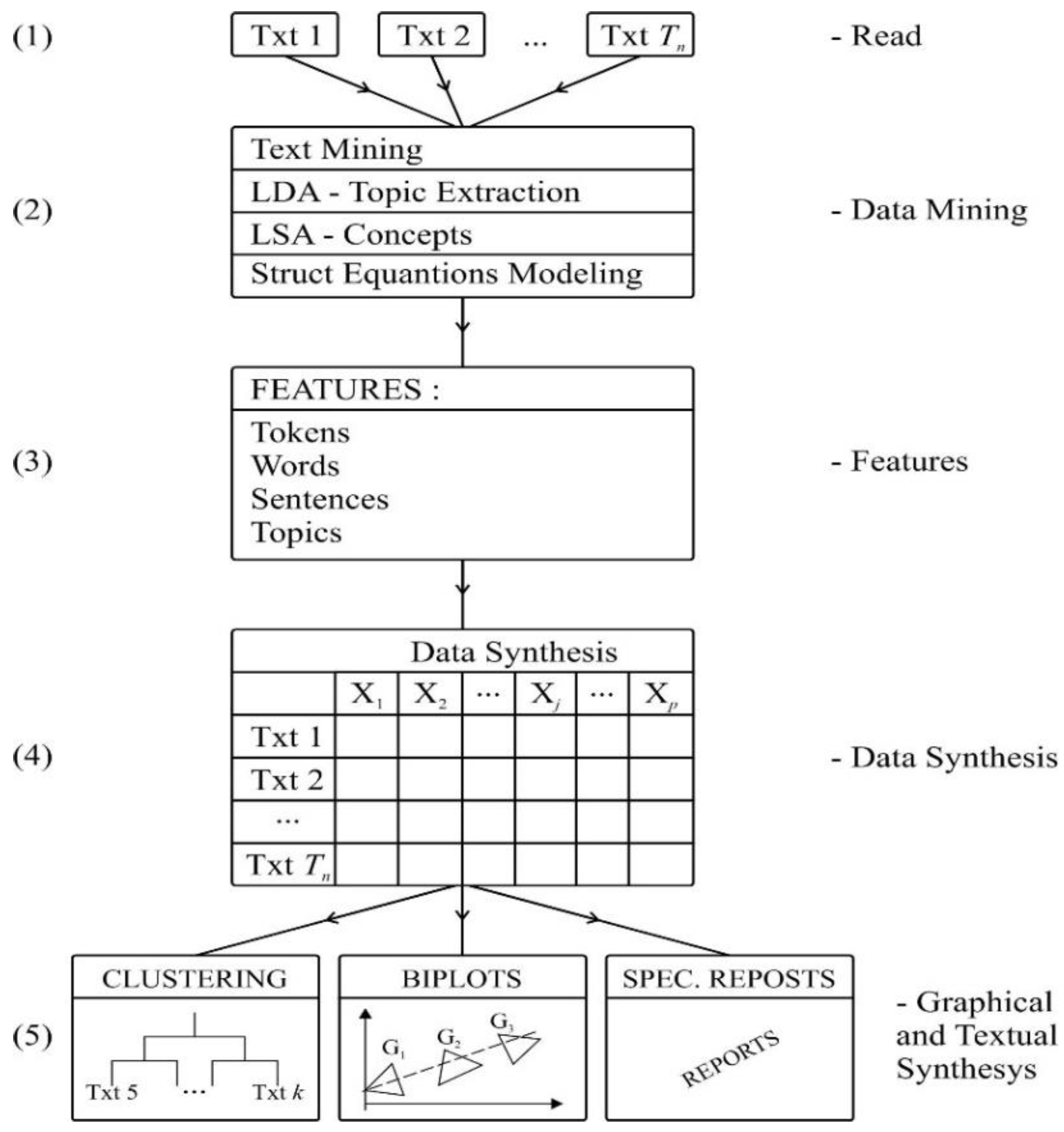
3.2. Methods: General View

Figure 1 shows the sequence of global steps leading from students’ texts to the graphical synthesis supporting teacher decision buildup.
(1)
Reading texts. Textual data sets containing the students’ answers are read. Generally, these texts are stored as separate text files (one file per text/student answer) forming a corpus, or the whole set of texts is stored as a sheet of an EXCEL book, one row per student/text, with an entire text stored in a single cell.
(2)
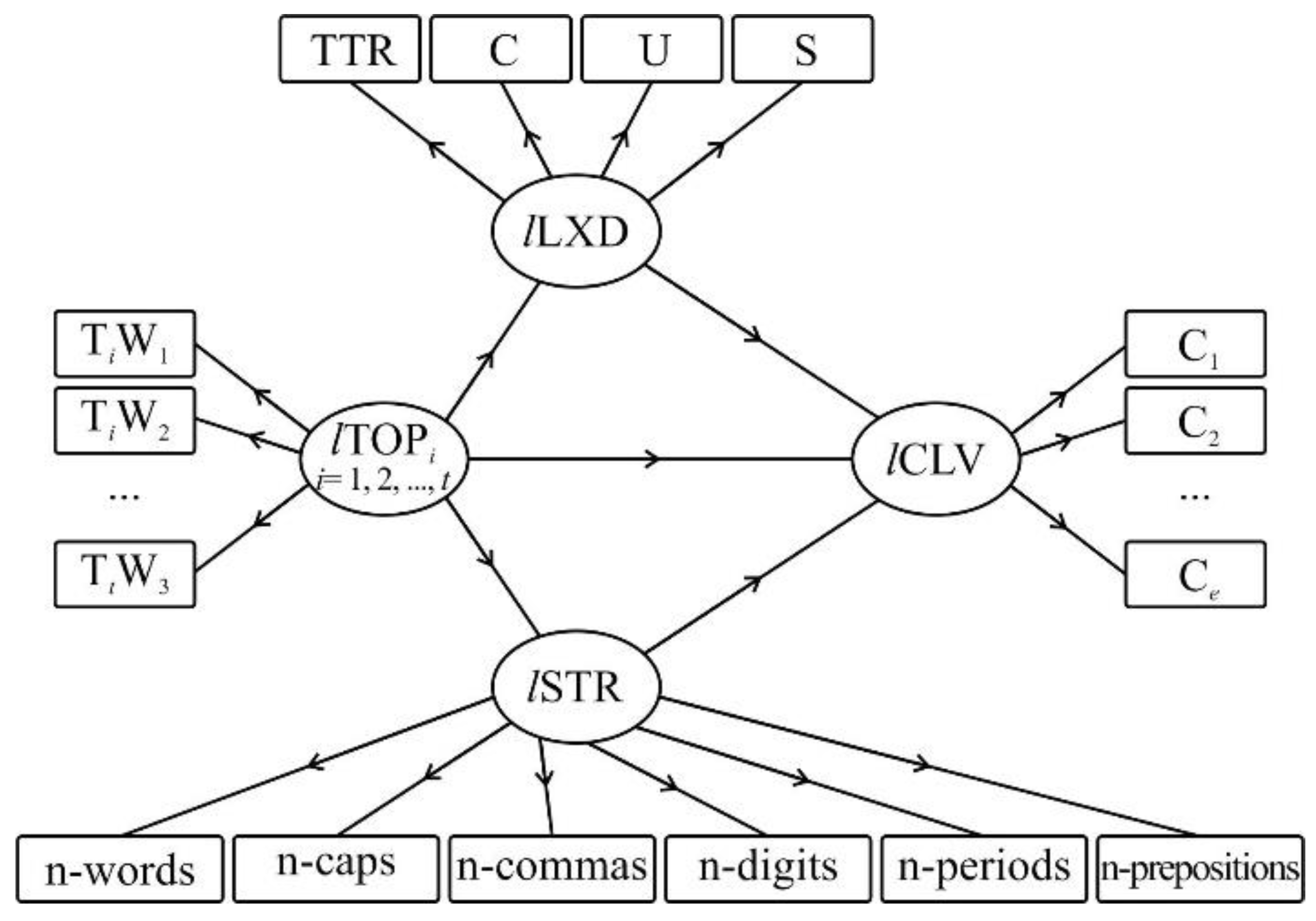
Textual data-mining tasks are performed with R packages—such as QuanteDa, LDA, LSA, PLS-PM and SemPLS (Ahadi et al., 2022) [38]. This analysis aims to obtain relevant information about students’ use of language in text construction. For example, token extraction (words, forms, sentences, pairs of words and their frequencies). Estimating topics subjacent to text construction is also considered using the LDA package (Chang, 2015) [39]. A theoretical model relating latent students’ skills in text and content construction with students’ competence in the subject matter is modelled using path modelling.
(3)
This step leads to the characterisation of each text by a set of feature values resulting from the previous text-mining analysis. Specific features are used to create partial reports to be used when a deeper analysis is necessary—to break ties, for example—and in the construction of global graphical and numeric synthesis.
(4)
Current Data Synthesis (CDS)—As a result of previous steps, a synthesis table data set is built. Its rows correspond to students/texts, and its columns represent relevant features used to construct multivariant graphical displays helping teachers in the decision process.
(5)
Graphical and Textual Synthesis—The main outputs from the system are biplots and classification trees involving texts and other supplementary information about students—such as results obtained in previous tests or other observational annotations. Thus, it is believed that a teacher must combine, closely supported by the framework, his/her previous knowledge about students, specific domain knowledge and teaching experience with scoring.

3.3. Model Formulation Using Structural Equations Modelling (SEM)

Beliefs about the relations between texts and students’ latent skills are modelled using structural equations modelling (SEM)/path analysis. The main belief here is that a student’s latent skills explain the final form and content of composition texts and that the student’s latent competence level (lCLV) in a specific domain is predictable from the manifestations in that text of those constructs.
The idea of using latent variables to relate composition texts with latent intrinsic students’ skills—“trins”—goes back to Page [15,16,17] and is associated with the development of the first program of automatic essay scoring (Automatic Essay Assessor). The assumptions adopted in the present work are:
Assumption 1.
Assessment and the choice of performing instruments are the teacher’s responsibility. In this context, the objective of text descriptive statistics to be supplied to teachers is to provide reliable and valid summaries and graphical descriptions of these texts so that teachers can reliably build their own decision by combining those syntheses with their previous knowledge and beliefs.
Assumption 2.
The teacher aims to be able to detect or recognise within the student text the manifestation or evidence of certain intrinsic, intangible or latent traits that are relevant to the formation of his scoring decision.
Assumption 3.
For large subject matters in which natural language and text production have a dominant role, common skills and a global competence level matter for assessment. The general idea is that a student’s competence level (lCLV) in the subject matter can be assessed by two minimum sets of latent variables: a set of variables explaining the text form and a set of variables expressing its content (competence in organising ideas and the content of expressed ideas). It is assumed that language richness, structuring skills and content knowledge are the main intangible causes contributing to students’ competence level for that subject matter.
There are several models for SEM, the main distinction in relation to their estimation being the distinction between covariance based/normal distribution assumptions (such as the Joreskog approach) and those that are variance-based, such as those estimated by PLS (Partial Least Squares), and distribution free. In this work, the last family of models is adopted.
The model in Figure 2 was, mainly, empirically grounded on the authors’ teaching experiences in the described classroom context. The inclusion of topics as latent variables to address text content and their relations with other latent variables in the structural model resulted from authors’ beliefs, grounded in that practical experience. From the theoretical point of view, the ideas expressed in Olson et al. (1991) [40] and in Page (1966, 1967, 1968) [15,16,17] were a strong source of inspiration. Referring to Figure 2, presenting a rough first model for these ideas, the meaning of the used symbols is:
lLXD—Latent variable Lexical Diversity LXD (student language richness or diversity).
lSTR—Latent variable Structuring Skill STR (student capability in structuring texts).
lCLV—Latent variable CLV (student level of competence in the subject matter).
lTOPj—Latent variables lTOP1 to lTOPt (student capability to use specific Topics) (j = 1 … t) in text construction.
In a reflective way, the manifest variables associated with those LVs are grouped in the following rectangular observation blocks in Figure 2:
Block 1—(See Figure 2—rectangles on the top side).
Formed by the manifest variables associated with latent lLXD.
In the expressions that follow, borrowed from Michalke (2020) [41] “V” is the number of types occurring among the total number of tokens (N).
T T R Type / Token   Ratio   ( T T R = V N ) .
C Hedran s   C   ( C =   l o g V l o g N ) .
S Summer   Index   ( S = l o g l o g V l o g l o g N ) .
U Dugast s   Uber   Index   ( u = l o g N 2 l o g N l o g V ) .
Block 2—(See Figure 2—rectangles on the bottom side).
Formed by the manifest variables associated with latent lSTR.
The following manifests are borrowed from Kearney & Hvitfeldt (2019)’s R package Text Features [42]:
n-words—Number of words in the composition text.
n-caps—Number of words in the composition text.
n-commas—Number of commas.
n-periods—Number of periods.
n-digits—Number of digits.
n-prepositions—Number of prepositions.
Block 3—(See Figure 2—rectangles on the right-hand side).
Formed by the manifest variables associated with the latent higher-order variable lCLV; in this work, these manifest variables are c1, c2, … ck, the first principal components from the other blocks (Sanchez, 2013) [43]. See also Sarstedt et al. (2019) [44] for other methods.
Block j (j = 4 … 4 + t)—(See Figure 2—rectangles on the left-hand side).
Formed by the manifest variables corresponding to each one of the t latent topics lTOPj (j = 1 … t)—For example, for lTOPj, the corresponding manifests are labelled TjW1, TjW2, … TjWnj. Those manifest variables are lists of words that indicate the presence or influence, in an observed composition text, of a specific latent topic lTOPj (j = 1 … t).
In this work, lTOPi (i = 1 … t) are latent variables that contribute significantly or explain the text’s formation. These lists can be short or long, depending on the concept whose influence is to be accounted for. For example, in the first data set, relative to Portuguese Literature and specifically to Saramago’s book Memorial do Convento, the teacher may be interested in knowing if the topic “love” is relevant to the meaning of a specific student text. This can be detected by the presence of lists of words such as “Baltazar, Blimunda, love” in that text.
Figure 2 accounts for the hypothesis that latent topics lTOPICj (j = 1 … t) influence both lLXD and lSTR. The following arguments can justify these assumptions: If a specific latent topic has an important place in the student’s mind, this will affect both the observed resulting text structure and the variety of words used in its construction, eventually reducing word variety. On the other hand, if the reverse was true (latent topic with weak relevance in the student’s mind), this would lead to a weak influence of this topic in the structuring of texts and to more lexical variety, now less conditioned by that specific latent topic. In this context, two hypotheses emerge (see Figure 2): H1—A strongly influent latent topic weakens the influence of lLXD, leading, counter-intuitively, to an expected negative correlation amongst those variables; H2—A strongly influent latent topic strengthens the influence of structuring skill lSTR in the production of observed texts (expected positive correlation).
Figure 2 expresses a dynamic schema with a varying structure, dependent on current teacher choices of number, content and meaning of latent topics. This means that Figure 2, more than a specific static model, represents a general family of models or modelling frameworks to be adapted to specific needs. To include a new topic in this framework is equivalent to asking some new specific question concerning students’ behaviour, whose answer is manifested in the frequency of occurrence of words associated with that new topic. The specific topics to be included in the model depend on the teacher’s experience, subject matter, school contingencies, discipline, teaching process time and questions whose answers the teacher is seeking. This means that specific topic inclusion allows some kind of “experimentation” with the available observational text data. This fact also results from the exogenous nature of these variables in the model, depending entirely on the teacher’s choices, in contrast with other latent variables whose presence expresses scientific and stable theories. In the analysis of all three data sets, it is assumed that the teacher was interested in knowing if three specific topics (t = 3), each one to be manifested in three (nj = 3) distinct lists of words, were present at the time of the creation of those texts.

3.4. Methods: Text Mining Summarising of Data Sets

Beliefs about the relations between texts and students’ latent skills are modelled using structural equations modelling (SEM)/path analysis.
One important resource of R text mining packages is the so-called document by features matrix (dfm), containing, for each text in the corpus and each word in the text, the frequency of that word in the text. This is the starting point for a rich set of possible reports and studies that can be adapted to the teacher’s needs (for the second data set, this matrix has 41 rows (texts) and 1498 columns or words).
Statistical text summarisation is an important input for teacher grading decisions. For example, Table 2 and Table 3 below present illustrations of summaries that can be helpful in the case of the R package QuanteDa (Benoit et al., 2018) [28].
Table 3 shows, for the set of 41 texts of data set 3, the 10 most frequent words. Note that if syntax errors were not corrected, as in this case, this list shows all words, including the wrong ones.

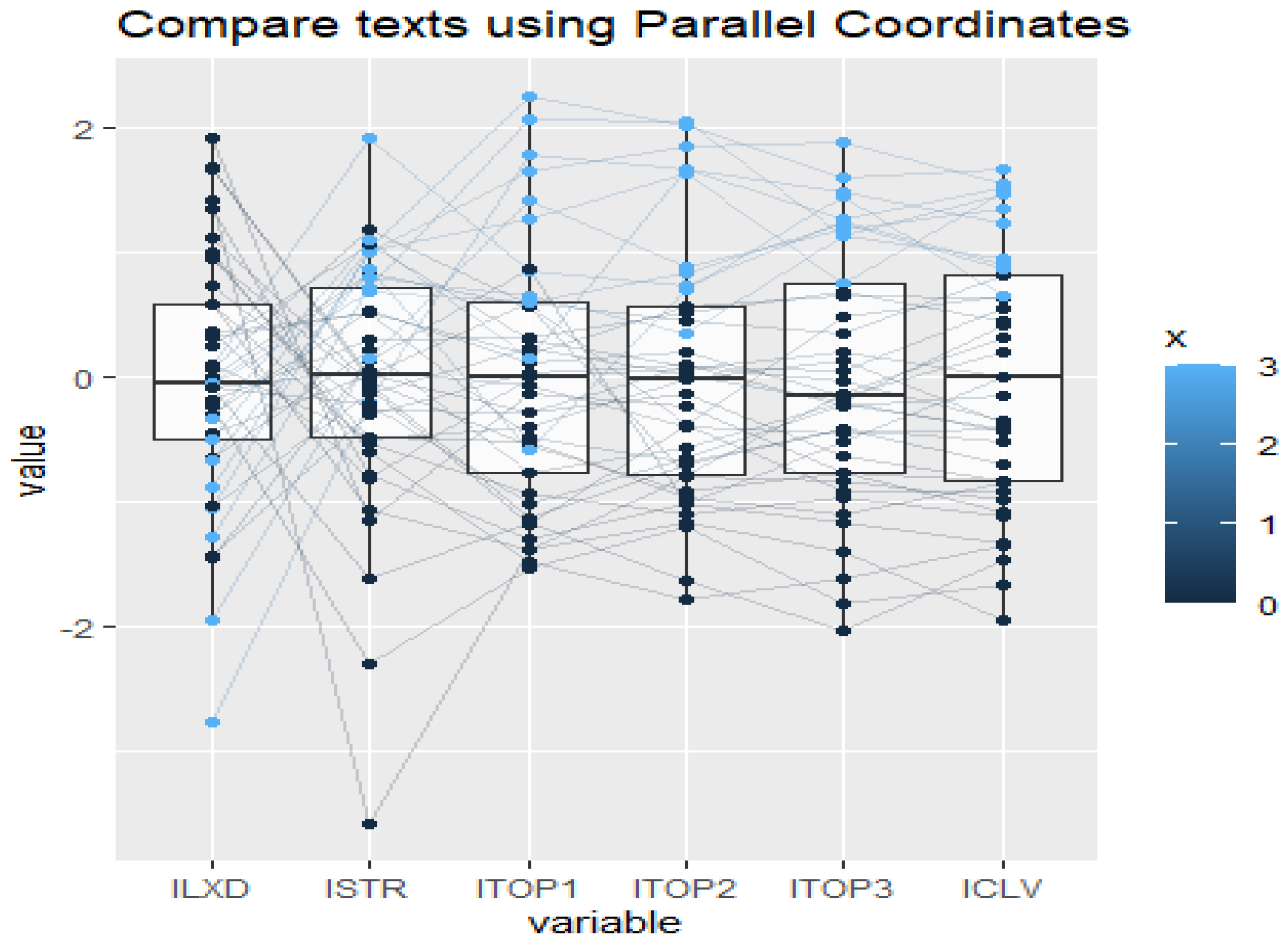
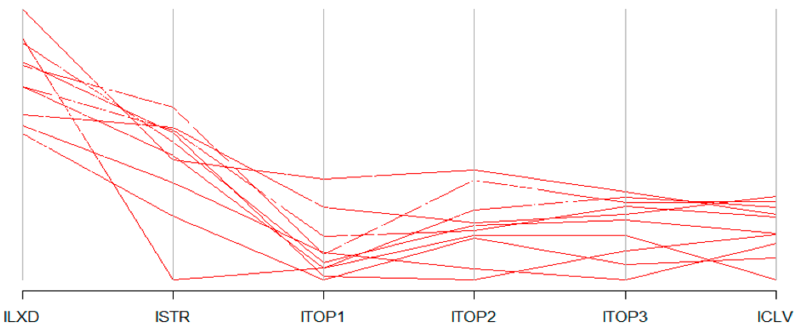
3.5. Methods: Graphical Methods

The three main classes of graphs selected to build the interface with teachers are:
1-Parallel coordinates plots, 2-Classification trees and 3-Biplots.
These graphs were chosen by the relevance of their properties to the tasks of comparing texts, identifying text patterns and relating texts with other variables relevant to scoring tasks. These aspects are illustrated as follows:
a—Parallel Coordinates Plots (Schloerke et al., 2020; Wickham, 2014; Venables & Ripley, 2002; Wegman, 1990) [45,46,47,48].
This kind of plot is illustrated in Figure 3, Figure 4, Figure 5 and Figure 6, obtained with the R package GGally (Schloerke et al., 2020) [45] with results from the analysis of data set 3. In each figure, a text is represented by a trajectory defined by the estimated values it assumes for each defined latent variable (lLXD, lSTR, lCLV, lTOPIC1, lTOPIC2, lTOPIC3). This allows, by interactive visual inspection, to compare the observed texts using those estimated values, easily detecting the main differences and their causes.
With this kind of plot, it is possible to address the following questions: if texts are sorted using the values of a specific variable—for example, variable lCLV—are there other variables that lead to similar orders for those texts? For example, Figure 3, Figure 4, Figure 5 and Figure 6 suggest that if texts are grouped by the quartiles of lCLV, those texts appear also, approximately, sorted on the quartiles of the other variables.
This graph also allows the study of specific groups of texts obtained by cluster analysis or by an arbitrary text selection in which the teacher is interested.
b—Classification Trees. Cluster Analysis
Figure 7 shows the hierarchical classification tree for 41 texts of data set 3 (university, economics). The vertical axis expresses a dissimilarity index (the higher the level, the more distinct the texts are). This tree was built using the R package Tree (Ripley, 2019) [49].
Here the trees, once built, can be cut at a level chosen by the user, allowing him or her to see if the internal homogeneity (similarity of student’s texts) is enough for his/her decision and to experiment with another in case of unacceptable variability calculated by the algorithms and compared with the teacher’s prior knowledge of students. This means that, as a purely exploratory method, there is no prior specification of the number of classes or other hyperparameters.
Bisecting this tree by an arbitrary horizontal line at a specific dissimilarity in the left vertical axis, the whole set of texts is divided into a specific number of clusters. For example, by bisecting at a level of 8, three clusters emerge. Reading Figure 7 from left to right, the first cluster includes all texts from the sequence {6, 11, 39, … 29}, the second one includes the texts {26, 13, 28, … 30} and the third, texts {8, 15, 39, … 20}. This means that, at a level of dissimilarity of 8, it is not possible to distinguish the texts within each one of these clusters; this suggests that, from the point of view of the six variables mentioned, it makes sense to roughly allocate the same mark to all. To distinguish the texts within each cluster, it would be necessary to bisect the tree at a lower level, corresponding to a lower dissimilarity, and consequently, to a higher mutual similarity. At the lowest level (0), all texts are distinct from all the others. Given a specific level, a good way to observe what separates a cluster from the other is to calculate basic statistics for all those six variables or relevant external variables and see what separates one group from the other.
c—Biplots
Given their general interpretability characteristics, biplots were selected as the main interaction method with the user (the teacher). For the classroom context, the number of observations is the number of students in the class (frequently below 100 texts), with biplots being used here to summarise the results of structural equations pls estimations. This means that the number of variables involved—the number of latent variables estimations in the model—is always small; 6, in the examples. In this specific context, the combined effect of these facts is that biplots always represent a very large percentage of information from data to be plotted: frequently above 80%, which guarantees reliable interpretations (Gabriel, 1971; Galindo-Villardón, 1986) [50,51].

4. Results of Data Analysis

A synthesis comparing data analysis results from data sets 1, 2 and 3, using the proposed methodology, is presented. Although the data sets have very distinct origins, corresponding to distinct teaching levels, and refer to distinct knowledge domains, the results (in what relates to performance and structure) are similar. This encourages further development and tests, including an operational test using software to be developed.

4.1. PLS Path Model Estimation Using PLS

In this work, the R package SemPLS was used for PLS estimation of structural equations in models of Figure 2. (Monecke & Leisch, 2012; Sanchez, 2013; Sarstedt et al., 2019) [43,44,52].
Table 4 contains indicator loadings estimation for the measurement model and path coefficients estimations for the structural model shown in Figure 2 for data sets 1, 2 and 3.
Table 5 shows global performance measures for that model, such as R2, Goldstein index, communality, and goodness of fit (Monecke & Leisch, 2012; Sanchez, 2013; Sarstedt et al., 2019) [43,44,52].
As previously mentioned, those three data sets were obtained in a fully independent way: unrelated observers obtained them in entirely separate school years (2008, 2017, 2020) for distinct subject matters (Portuguese literature, sociology, economics) and different school systems and places. It must also be stressed that lTOPi (i = 1 … t) latent variables have meanings and indicator lists of r words which are completely distinct and unrelated.
As seen from Table 5 and Table 6, the estimation results are very similar for the three data sets and coherent; also, see below that the topology of biplots synthesising these results is almost identical.
To sum up, all these findings, supported by the available data, suggest that the present method addresses or is sensitive to some subjacent invariant reality clearly related to the aims of this work.

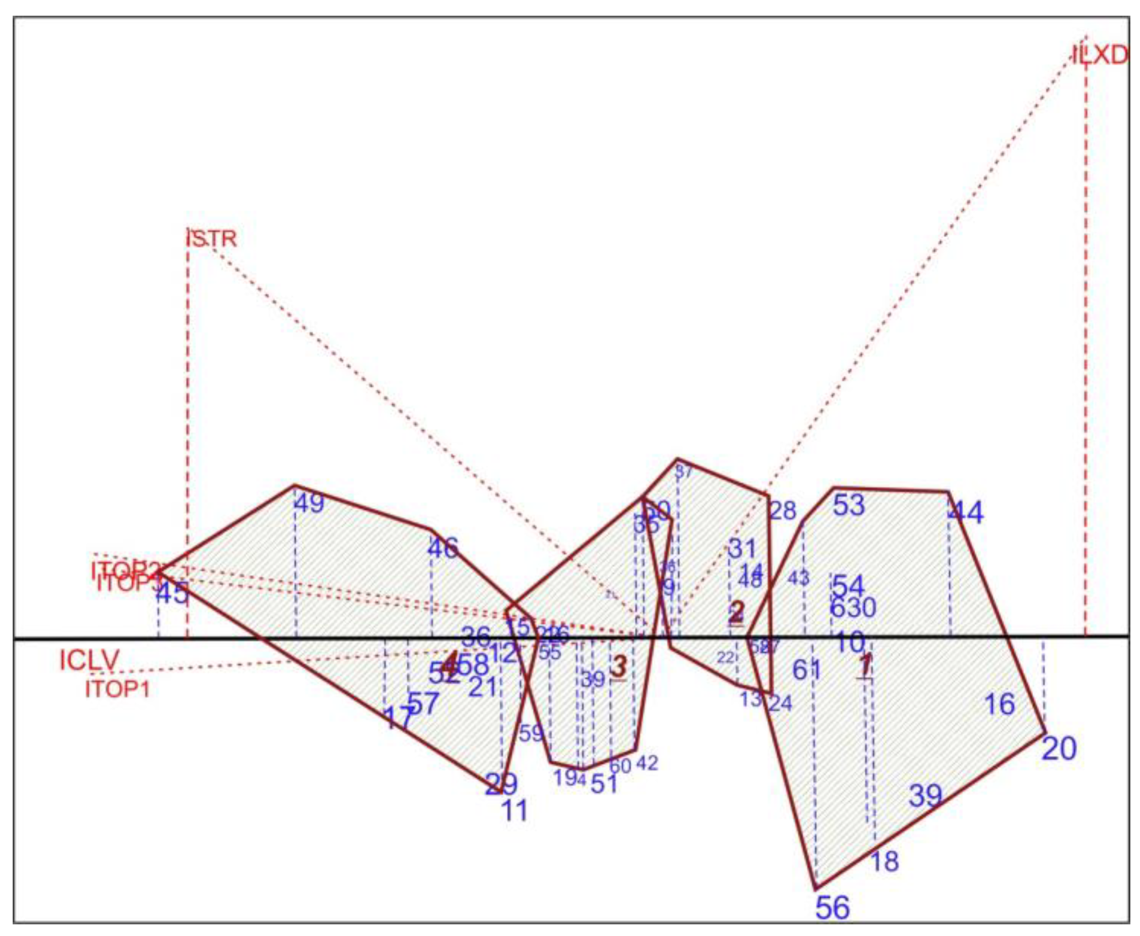
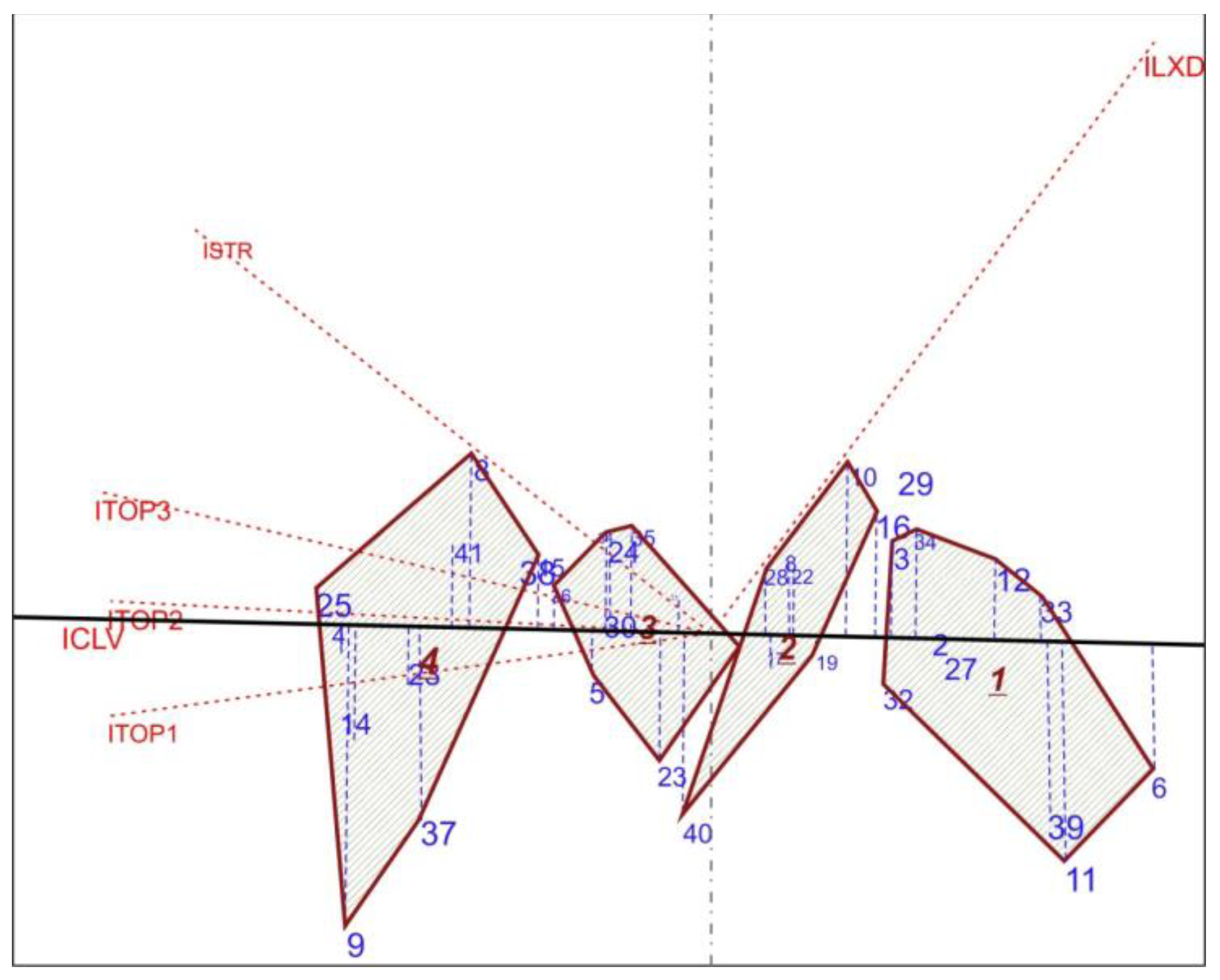
4.2. Text Comparisons Using Biplots

PLS estimations of six latent variables (p = 6) involved in Figure 2 are collected in three intermediate data sets with dimensions 61 × 6, 24 × 6 and 41 × 6, corresponding to each one of the datasets described in Table 1. These three data sets are transformations of the original data sets through the path model and its estimation using PLS. These transformed data sets are summarised using HJ-Biplots plotted in Figure 8, Figure 9 and Figure 10 (Galindo-Villardón, 1986) [51]. See Figure 1 (4) Data Synthesis and (5) Graphical and Textual Synthesis.
As explained before, in this context, 2D biplots explain almost all the variance of those data sets since, at most, the biplot dimension is max (n rows, p columns).
Figure 8 shows one possible interactive implementation of these ideas, using the BiplotsPMD program (Vairinhos, 2003) [53], working with data set 2. In future implementations of the framework, the user will be allowed to define the model that best suits local needs and previous experience gained with specific student populations. This means specifying the model’s variants in Figure 2 with latent topics and the lists of words that form its manifest variables.
The model estimated parameters are included in the so-called current data synthesis (CDS), Figure 1, (5). The study to suggest marks to texts can now proceed, namely, through the production of biplots, other graphics and tables in response to questions issued according to the teacher’s needs. Figure 1, (5)—Graphical and Textual Synthesis.
Figure 8, Figure 9 and Figure 10 display biplots produced to summarise the transformed data set 2 (24 texts from vocational-technical students), data set 1 (61 texts from the 12th year of the official system, literature) and data set 3 (41 texts of a first-year university management course, subject: economics).
Projecting the texts orthogonally on the direction of variable lCLV, a text ordination is obtained that can be supplied to the teacher as a first crude clue for text marks. This makes sense given the small percentage of variance not explained by those biplots (about 10%).
In the case of data set 2 (Figure 8) the suggested order for the texts is, from right to left in Figure 8: 14 (worst) < 18 < 4 < 22 < 16 < 6 < 12 < 3 < 21 < 7 < 1 < 2 <……< 13 < 23 < 19 < 5 < 8 < 11 (best).
Figure 9 and Figure 10 show, for data sets 1 and 3, the corresponding suggestions for text ordinations.
Those figures present, also, the convex polygons corresponding to the quartiles of lCLV values, numbered from right to left by quartile number 1, 2, 3, 4.
Despite the diversity of texts used, obtained in completely different learning environments, addressing very different subject matter (sociology, economics, literature) and corresponding to very distinct time frames, the topology of obtained biplots is, surprisingly, similar. Specifically: the percentage of information explained both by the whole biplots and the horizontal and vertical axis is almost the same for the three data sets: ~90% = 80% + 10%. In the three cases, lSTR and lLXD are almost orthogonal (suggesting that the lexical richness is independent of structuring text capability). Moreover, the topics are highly correlated, for the three studies, presenting a negative correlation with lLXD (lexical richness), which is coherent with the assumptions used for model 2.
In the three studies, the estimated lCLV latent variable forms a very small angle with the horizontal axis (first principal component), meaning that the contrast left-right is highly meaningful in explaining differences in text quality (measured by lCLV).

5. Reliability and Validity Issues

This work proposes a framework, based on text mining, to help teachers score OEQ answer texts in a classroom context. This means that the objective is not to obtain automatic classifications but to present to the teacher, in real time, a faithful synthesis of those texts, allowing him or her to supply the text’s marks with a minimum workload.
Also, reliability and validity issues associated with this framework must address problems of efficiency and effectiveness related to teacher time economy more than the question of showing that the marks allocated in this way have a high correlation with “true” (unknown and unobservable) student skills. This is because the final marks result from a decision of the teacher, built from the clues, statistical facts and summarisations suggested by the system.
A true validity and reliability study of this framework can only be performed in the context of experiences with its use in real schools, using supporting software implementing the framework, in a real teaching context, with real students, during a large enough time interval. This kind of experience is only possible with the help of educational system authorities and the participation of several schools.
When true scores by a teacher are available, it is important to compare them with the suggested ordinations of texts obtained using the present framework. In this case, latent variable lCLV (Competence Level) is, by construction, explained by content lTOPi (i = 1 … t) and intrinsic characteristics (lLXD and lSTR). It is natural that its estimated values are used to suggest rough clues about the value of the texts, as explained.
Specifically, in the present investigation, for data set 1 (official examinations, secondary studies, Portuguese literature) and data set 3 (formative testing, economics, first year), final scores allocated by teachers were available. This allowed us to compare these scores with the rough clues suggested using variable lCLV estimations and obtain the correlations, for each data set, between those human-made marks and the suggested clues obtained from lCLV estimations. For data set 1, an additional set of scores obtained from a hired Portuguese teacher was available (HIR).
For data set 1, correlations among available human correctors classifications (OFFICIAL and HIR) and values of lCLV can be seen in Table 6.
Surprisingly, the correlation between scores allocated by the official human correctors and those obtained by a Portuguese teacher hired by the second author is not only low (0.462) but of the same magnitude as those obtained between those human correctors and the estimations of lCLV. This same pattern occurs with data set 3 in a distinct learning setting (subject matter, very distinct learning level and time interval between observations of some years); for data set 3, the correlation between teacher scores and estimations of latent variable lCLV is 0.497.
For data set 3, the correlation between teacher classifications and variable lCLV estimation was coherent with those obtained for data set 1.
Text classifications for data set 2 were not available. However, the teacher has informed the authors of this work that the ordination obtained with the framework coincided—up to two differences—with the true teacher scores.
Figure 11a,b show, for data sets 1 and 3, a comparison between standardised distributions of marks supplied by human teachers and lCLV. In both cases, the hypothesis of equal distributions was not rejected by the Kolmogorov–Smirnov test at the 0.01 level. For data set 1, correlation = 0.433; Kolmogorov–Smirnov Test p value = 0.125. For data set 3 correlation = 0.497; Kolmogorov–Smirnov Test p value = 0.772.

6. Discussion

The proposed framework is the result of an exploratory effort to respond to a well-known problem: the potential of open-ended questions (OEQ) as teaching and learning tools is enormous, but the possibility of its routine use is contradicted and even hindered by the enormous effort to evaluate the texts.
When trying to formulate a preliminary model for this problem, a basic perception is that, when the teacher tries to score texts, what he or she seeks is, basically, to detect in the texts produced by the students, signs of certain hidden skills. Does a certain text “signal” that the student sought to convey a certain idea relevant to the learning process? Was the student sensitive to a certain concept considered important by the teacher? Does the text suggest that the student has a good ability to organise ideas or even to generate lexical innovations?
In other words: the two basic questions that emerge when scoring texts are whether, yes or no, there are traces of certain concepts or certain general skills, such as the presence of specific concepts, the ability to structure ideas or the mastery of language, which is in line with the work of Grover et al. (2015) [54] and Yeung (2018) [55]. The methodology of structural equations occurs in this context as an adequate modelling instrument, linking the observed texts to the latent capacities whose traits are being sought to detect. In particular, the concept of “topic”, modelled as a latent variable characterising text content, has proved to be very flexible since it allows adapting the model to diverse disciplines with a common teaching language, such as English, history, sociology, and psychology. The framework is the same, but the number and meaning of the topics to use in the model vary with the specific modelling needs.
In this context, more than specialised literature, the experience and beliefs of the authors resulting from many years of experience in the classroom were decisive in structuring this tentative model.
Once the estimates of the latent variables, topics, and others, have been obtained from available texts, it is necessary to present the results to the teacher (Munroe, 2015) [56], so that it is easy for him or her to capture the essence and combine this evidence with his or her own knowledge and perceptions about of the students and the environment (Hamit, 2018) [57]. For this, graphical methods of multivariate data synthesis, such as biplots, classification trees and others were the preferred method.
According to our results, the estimates of the structural model and performance indicators are coherent for the three available data sets, obtained in schools of different levels, at different times and with very different students.
The same happens with the picture displayed in Figure 8, Figure 9 and Figure 10 representing the texts on biplots relating those texts (students) with the latent variables (topics and other) used in the model: the structure of those biplots (defined by angles between latent variables) are very similar despite the heterogeneity of available texts, suggesting that there is some invariant subjacent to these results.
The results obtained are exploratory and observational in nature, not experimental data, meaning that, at this stage of the project, it is too soon to draw final conclusions. However, the results obtained encourage future research in this direction, namely, to develop software that can support a large-scale experience, covering several schools for at least a full academic year.

7. Conclusions and the Future Work

It is assumed that teachers are responsible for teaching and evaluating in the context of a classroom and formative evaluation. It is also assumed that teachers are entitled to choose the methods and tools they feel better using, in order to accomplish their duties.
This choice may eventually include automatic classification systems. This means that, from this perspective, the “replacement” of teachers with computers is not an option. This does not eliminate the need for some degree of administrative uniformity or teacher advice in choosing those instruments and procedures. In this context, the paper suggests a framework, based on the OEQ texts’ descriptive statistics, aiming to reduce the teachers’ grading effort and, consequently, increase the use of OEQs as much as possible.
The framework must be adapted for each specific subject, including the choice of appropriate numbers and topics and their meaning.
It was observed that when the suggested method was applied to texts obtained in diverse settings (learning system, subject matter, type of evaluation, academic year), the results are similar. In particular, the topology of biplots obtained was almost identical. A full-scale future validation will only be possible as part of an experiment involving enough schools during a school year, using an interactive software implementation of the framework; meanwhile, the results obtained show encouraging signs of feasibility for the proposed framework.
It was found that the correlation between official classifications of texts available and those assigned by a Portuguese teacher hired by this project was of the same magnitude as the correlations obtained between those teachers and results obtained with the framework. It was also found that the distributions of standardised results obtained by the teachers and suggested by the framework were not significantly distinct.
The main limitations of the present work are the small size of corpora available and the need to perform a full-scale experiment, involving several schools during an academic year, supported by a software implementation of presented ideas.

Author Contributions

Conceptualization, V.M.V.; Writing—original draft, V.M.V. and F.M.; Writing—review and editing, V.M.V. and F.M.; resources and data curation, F.M., L.A.P. and H.N.; Methodology, V.M.V., C.P. and P.G.-V.; Formal analysis and supervision, V.M.V., F.M., C.P. and P.G.-V. All authors have read and agreed to the published version of the manuscript.

Funding

This research received no external funding.

Conflicts of Interest

The authors declare no conflict of interest.

References

  1. Livingston, S.A. Constructed-Response Test Questions: Why We Use Them; How We Score Them. RD Connect. 2009, 11. [Google Scholar]
  2. McClellan, C. Constructed-Response Scoring—Doing It Right. RD Connect. 2010, 13, 1–7. [Google Scholar]
  3. Li, H.; Cai, Z.; Graesser, A.C. Computerized summary scoring: Crowdsourcing-based latent semantic analysis. Behav. Res. Methods 2018, 50, 2144–2161. [Google Scholar] [CrossRef] [Green Version]
  4. Wiliam, D.; Lee, C.; Harrison, C.; Black, P. Teachers developing assessment for learning: Impact on student achievement. Assess. Educ. Princ. Policy Pract. 2004, 11, 49–65. [Google Scholar] [CrossRef]
  5. Feinerer, I.; Hornik, K.; Meyer, D. Text Mining Infrastructure in R. J. Stat. Softw. 2008, 25, 1–54. [Google Scholar] [CrossRef] [Green Version]
  6. Lebart, L.; Salem, A.; Berry, L. (Eds.) Exploring Textual Data; Springer: Heidelberg, The Netherlands, 1998; Volume 4. [Google Scholar] [CrossRef]
  7. Süzen, N.; Gorban, A.N.; Levesley, J.; Mirkes, E.M. Automatic short answer grading and feedback using text mining methods. Procedia Comput. Sci. 2020, 169, 726–743. [Google Scholar] [CrossRef]
  8. Landauer, T.K. Automatic Essay Assessment. Assess. Educ. Princ. Policy Pract. 2003, 10, 295–308. [Google Scholar] [CrossRef]
  9. Landauer, T.K.; Dumais, S.T. A solution to Plato’s problem: The latent semantic analysis theory of acquisition, induction, and representation of knowledge. Psychol. Rev. 1997, 104, 211–240. [Google Scholar] [CrossRef]
  10. Landauer, T.K.; Laham, D.; Rehder, B.; Schreiner, M.E. How Well Can Passage Meaning be Derived without Using Word Order? In A Comparison of Latent Semantic Analysis and Humans, Proceedings of the 19th Annual Conference of the Cognitive Science Society; Shafto, M.G., Langley, P., Eds.; Lawrence Erlbaum Associates: Mahwah, NJ, USA, 1997; pp. 412–417. Available online: http://lsa.colorado.edu/papers/cogsci97.pdf (accessed on 25 October 2022).
  11. Landauer, T.K.; McNamara, D.S.; Dennis, S.; Kintsch, W. (Eds.) Handbook of Latent Semantic Analysis; Psychology Press: Hove, UK, 2007. [Google Scholar] [CrossRef]
  12. Shermis, M.D.; Shneyderman, A.; Attali, Y. How important is content in the ratings of essay assessments? Assess. Educ. Princ. Policy Pract. 2008, 15, 91–105. [Google Scholar] [CrossRef]
  13. Ke, Z.; Ng, V. Automated Essay Scoring: A Survey of the State of the Art. In Proceedings of the Twenty-Eighth International Joint Conference on Artificial Intelligence, Macao, China, 10–16 August 2019; pp. 6300–6308. [Google Scholar] [CrossRef]
  14. Perin, D.; Lauterbach, M. Assessing Text-Based Writing of Low-Skilled College Students. Int. J. Artif. Intell. Educ. 2018, 28, 56–78. [Google Scholar] [CrossRef]
  15. Page, E.B. The Imminence of Grading Essays by Computer. Phi Delta Kappan 1966, 47, 238–243. Available online: https://www.jstor.org/stable/20371545 (accessed on 25 October 2022).
  16. Page, E.B. Statistical and linguistic strategies in the computer grading of essays. In Proceedings of the 1967 Conference on Computational Linguistics, Stroudsburg, PA, USA, 23–25 August 1967; pp. 1–13. [Google Scholar] [CrossRef] [Green Version]
  17. Page, E.B. The Use of the Computer in Analyzing Student Essays. Int. Rev. Educ. 1968, 14, 210–225. Available online: https://www.jstor.org/stable/3442515 (accessed on 25 October 2022). [CrossRef]
  18. Page, E.B. Project Essay Grade: PEG. In Automated Essay Scoring: A Cross-disciplinary Perspective; Shermis, M.D., Burstein, J.C., Eds.; Lawrence Erlbaum Associates: Mahwah, NJ, USA, 2002; pp. 43–54. [Google Scholar]
  19. Page, E.B.; Poggio, J.P.; Keith, T.Z. Computer Analysis of Student Essays: Finding Trait Differences in Student Profile. In Proceedings of the Annual Meeting of the American Educational Research Association, Chicago, IL, USA, 21–26 April 2022. [Google Scholar]
  20. Deerwester, S.; Dumais, S.T.; Furnas, G.W.; Landauer, T.K.; Harshman, R. Indexing by latent semantic analysis. J. Am. Soc. Inf. Sci. 1990, 41, 391–407. [Google Scholar] [CrossRef]
  21. Dikli, S. Automated Essay Scoring. Turk. Online J. Distance Educ. 2006, 7, 49–62. [Google Scholar]
  22. Bellegarda, J.R. Latent Semantic Mapping: Principles & Applications; Springer International Publishing: New York, NY, USA, 2007. [Google Scholar] [CrossRef]
  23. Pereira, L.A.P.d.M.A. Contribuição Para A Formulação De Uma Metodologia De Ensino E Avaliação Baseada na Análise Estatística de Textos em Português; Faculdade de Ciências Sociais e Humanas, Universidade Nova de Lisboa: Lisboa, Portugal, 2013; Available online: http://hdl.handle.net/10362/12100 (accessed on 25 October 2022).
  24. Kerkhof, R.G. Natural Language Processing for Scoring Open-Ended Questions: A Systematic Review. Available online: http://essay.utwente.nl/82090/ (accessed on 25 October 2022).
  25. Liu, S.; Zeng, S.; Li, S. Evaluating Text Coherence at Sentence and Paragraph Levels. arXiv 2020, arXiv:2006.03221. [Google Scholar]
  26. Pietsch, A.-S.; Lessmann, S. Topic modeling for analyzing open-ended survey responses. J. Bus. Anal. 2018, 1, 93–116. [Google Scholar] [CrossRef] [Green Version]
  27. Roberts, M.E.; Stewart, B.M.; Tingley, D.; Lucas, C.; Leder-Luis, J.; Gadarian, S.K.; Albertson, B.; Rand, D.G. Structural Topic Models for Open-Ended Survey Responses. Am. J. Political Sci. 2014, 58, 1064–1082. [Google Scholar] [CrossRef] [Green Version]
  28. Benoit, K.; Watanabe, K.; Wang, H.; Nulty, P.; Obeng, A.; Müller, S.; Matsuo, A. Quanteda: An R package for the quantitative analysis of textual data. J. Open Source Softw. 2018, 3, 774. [Google Scholar] [CrossRef] [Green Version]
  29. Burrows, S.; Gurevych, I.; Stein, B. The Eras and Trends of Automatic Short Answer Grading. Int. J. Artif. Intell. Educ. 2015, 25, 60–117. [Google Scholar] [CrossRef] [Green Version]
  30. Galhardi, L.B.; Brancher, J.D. Machine Learning Approach for Automatic Short Answer Grading: A Systematic Review; Springer: Berlin/Heidelberg, Germany, 2018; pp. 380–391. [Google Scholar] [CrossRef]
  31. Paalman, J.; Mullick, S.; Zervanou, K.; Zhang, Y. Term Based Semantic Clusters for Very Short Text Classification. In Proceedings of the Natural Language Processing in a Deep Learning World; 2019; pp. 878–887. [Google Scholar] [CrossRef]
  32. Poulimenou, S.; Stamou, S.; Papavlasopoulos, S.; Poulos, M. Short Text Coherence Hypothesis. J. Quant. Linguist. 2016, 23, 191–210. [Google Scholar] [CrossRef]
  33. Zhang, L.; Huang, Y.; Yang, X.; Yu, S.; Zhuang, F. An automatic short-answer grading model for semi-open-ended questions. Interact. Learn. Environ. 2019, 30, 177–190. [Google Scholar] [CrossRef]
  34. Williamson, D.M.; Xi, X.; Breyer, F.J. A Framework for Evaluation and Use of Automated Scoring. Educ. Meas. Issues Pract. 2012, 31, 2–13. [Google Scholar] [CrossRef]
  35. Feathers, T. Flawed Algorithms Are Grading Millions of Students’ Essays. Available online: https://www.vice.com/en/article/pa7dj9/flawed-algorithms-are-grading-millions-of-students-essays (accessed on 20 August 2019).
  36. Lott-Lavigna, R. A-Level Students to Receive Their Predicted Grades in Government U-Turn. Available online: https://www.vice.com/en/article/y3ze87/a-level-students-to-receive-their-predicted-grades-in-government-u-turn (accessed on 17 August 2020).
  37. Rico-Juan, J.R.; Gallego, A.-J.; Valero-Mas, J.J.; Calvo-Zaragoza, J. Statistical semi-supervised system for grading multiple peer-reviewed open-ended works. Comput. Educ. 2018, 126, 264–282. [Google Scholar] [CrossRef]
  38. Ahadi, A.; Singh, A.; Bower, M.; Garrett, M. Text Mining in Education—A Bibliometrics-Based Systematic Review. Educ. Sci. 2022, 12, 210. [Google Scholar] [CrossRef]
  39. Chang, J. Lda: Collapsed Gibbs Sampling Methods for Topic Models (1.4.2). CRAN Repository. 2015. Available online: https://cran.r-project.org/package=lda (accessed on 25 October 2022).
  40. Olson, G.A.; Faigley, L.; Chomsky, N. Language, Politics, and Composition: A Conversation with Noam Chomsky. J. Adv. Compos. 1991, 11, 1–35. Available online: https://www.jstor.org/stable/20865759 (accessed on 25 October 2022).
  41. Michalke, M. Korpus: Text Analysis With Emphasis on Pos Tagging, Readability And Lexical Diversity (0.13-8). Available online: https://cran.r-project.org/package=koRpus (accessed on 25 October 2022).
  42. Kearney, M.W.; Hvitfeldt, E. Textfeatures: Extracts Features from Text (0.3.3). Available online: https://cran.r-project.org/package=textfeatures (accessed on 25 October 2022).
  43. Sanchez, G. PLS Path Modeling with R. 2013. Available online: https://www.gastonsanchez.com/PLS_Path_Modeling_with_R.pdf (accessed on 25 October 2022).
  44. Sarstedt, M.; Hair, J.F.; Cheah, J.-H.; Becker, J.-M.; Ringle, C.M. How to Specify, Estimate, and Validate Higher-Order Constructs in PLS-SEM. Australas. Mark. J. 2019, 27, 197–211. [Google Scholar] [CrossRef]
  45. Schloerke, B.; Cook, D.; Larmarange, J.; Briatte, F.; Marbach, M.; Thoen, E.; Elberg, A.; Toomet, O.; Crowley, J.; Hofmann, H.; et al. GGally: Extension to “ggplot2” (2.0.0). Available online: https://cran.r-project.org/package=GGally (accessed on 25 October 2022).
  46. Venables, W.N.; Ripley, B.D. Modern Applied Statistics with S; Springer: New York, NY, USA, 2002. [Google Scholar] [CrossRef]
  47. Wegman, E.J. Hyperdimensional Data Analysis Using Parallel Coordinates. J. Am. Stat. Assoc. 1990, 85, 664. [Google Scholar] [CrossRef]
  48. Wickham, H. Tidy Data. J. Stat. Softw. 2014, 59. Available online: http://www.jstatsoft.org/ (accessed on 25 October 2022). [CrossRef]
  49. Ripley, B. Tree: Classification and Regression Trees (1.0-40). 2019. Available online: https://cran.r-project.org/package=tree (accessed on 25 October 2022).
  50. Gabriel, K.R. The biplot graphic display of matrices with application to principal component analysis. Biometrika 1971, 58, 453–467. [Google Scholar] [CrossRef]
  51. Galindo-Villardón, M.P. Una alternativa de representación simultánea: HJ-Biplot. Qüestiió Quad. D’estadística I Investig. Oper. 1986, 10, 13–23. Available online: http://hdl.handle.net/2099/4523 (accessed on 25 October 2022).
  52. Monecke, A.; Leisch, F. Sempls: Structural Equation Modeling Using Partial Least Squares. J. Stat. Softw. 2012, 48, 1–32. [Google Scholar] [CrossRef] [Green Version]
  53. Vairinhos, V.M. Desarrollo de un Sistema de Minería de Datos Basado en los Métodos de Biplot. Ph.D. Tesis, Universidad de Salamanca, Salamanca, Spain, 2003. [Google Scholar]
  54. Grover, S.; Pea, R.; Cooper, S. Designing for deeper learning in a blended computer science course for middle school students. Comput. Sci. Educ. 2015, 25, 199–237. [Google Scholar] [CrossRef]
  55. Yeung, W.C. Embracing individual differences: Overview of classroom and curricular strategies with reference to the Hong Kong English language curriculum and assessment guide. Hong Kong Teach. Cent. J. 2018, 17, 125–144. [Google Scholar]
  56. Munroe, L. The open-ended approach framework. Eur. J. Educ. Res. 2015, 4, 97–104. [Google Scholar] [CrossRef]
  57. Hamit, O. A qualitative study of school climate according to teachers’ perceptions. Eurasian J. Educ. Res. 2018, 18, 81–98. [Google Scholar]
Figure 1. Diagram illustrating the process’s main tasks to generate the graphical synthesis of texts.
Mathematics 10 04152 g001
Figure 2. Measurement and Structural Model accounting for influences of Topics on Lexical Diversity-lLXD, Structuring Skill lSTR and lCLV (Competence Level).
Mathematics 10 04152 g002
Figure 3. Parallel coordinates graphs for the estimations of latent variables in the model in Figure 2. This plot was obtained with R package MASSGGally: ggparcoord.
Mathematics 10 04152 g003
Figure 4. With the data in Figure 3, texts belong to the first quartile of lCLV, R package MASS.
Mathematics 10 04152 g004
Figure 5. With the data in Figure 3, texts belong to the second quartile of lCLV, R package MASS.
Mathematics 10 04152 g005
Figure 6. With the data used in Figure 3, texts belong to the third quartile of lCLV, R package MASS.
Mathematics 10 04152 g006
Figure 7. Classification tree for data set 3 (University, Economics) obtained with R package tree.
Mathematics 10 04152 g007
Figure 8. Interactive drawing and study of HJ-biplots and clustering of texts belonging to data set 2, with 24 texts. Blue numbers mean texts. Red strings mean latent variables.
Mathematics 10 04152 g008
Figure 9. Interactive drawing and study of HJ-biplots and clustering of texts belonging to data set 1, with 61. Blue numbers mean texts. Red strings mean latent variables.
Mathematics 10 04152 g009
Figure 10. HJ-biplot and clustering of texts belonging to data set 3, with 41 texts in blue numbers and red strings as latent variables.
Mathematics 10 04152 g010
Figure 11. (a,b)—Obtained with R package ggplot2. (a) Data set 1: Kolmogorov test for teacher and lCLV standardised classifications distributions; (b) Data set 3: Kolmogorov test for HIP (hired teacher) and lCLV standardised classifications.
Mathematics 10 04152 g011
Table 1. Synthesis of features of data sets used for data analysis.
Data Set NameCorpusLevelUseSubject
Matter
ContextDate
Data Set 161 textsSec (12th year)SummativePortuguese
Literature
Official
Examinations
2008
Data Set 224 textsSec (12th year)FormativeSociologyIn the class2017
Data Set 341 textsUniversityFormativeEconomyIn the class2020
Legend—“Sec” means Secondary level of education.
Table 2. The ten most frequent words in data set 3.
FeatureFrequencyRankDocfreq
1economy205138
2is160233
3definition129327
4science108437
5object74530
6study71632
7social60727
8to be56824
9human55925
10production541028
Table 3. Partial view of tokens, types and sentences of 41 texts of the dataset, sorted by decreasing order of types.
TextTypesTokensSentences
6text651721
11text1154772
27text27681055
39text39701104
33text33841295
12text12851344
23text23871737
9text9892225
26text26981673
40text401001998
Table 4. Measurement model weights and structural model path coefficients estimates for the model in Figure 2 and for the data sets 1, 2 and 3. Using the bootstrap method with 500 pseudo-samples to obtain pseudo-confidence intervals, the symbol “ns” for some of the cells means that the corresponding values were considered non-significative at level 0.01.
Measurement Model
(Figure 2)
Data Set 1Data Set 2Data Set 3
TOP 1 ®T1W10.9110.9280.855
TOP 1 ®T1W20.676ns (0.01)0.801
TOP 1 ®T1W30.5710.7790.729
TOP 2 ®T2W10.9400.8630.894
TOP 2 ®T2W20.9220.9120.820
TOP 2 ®T2W30.597ns (0.01)0.647
TOP 3 ®T3W10.9240.9490.885
TOP 3 ®T3W20.7840.5710.768
TOP 3 ®T3W30.6420.6850.582
LXD ®C0.9950.9950.998
LXD ®Sns (0.01)0.8750.967
LXD ®TTR0.9720.9580.972
LXD ®U0.9150.9320.978
STR ®ncaps0.860.8560.840
STR ®ncomm0.8320.8540.851
STR ®ndig0.7880.427ns (0.01)
STR ®nperiod0.9480.8520.664
STR ®npropns (0.01)0.3800.548
STR ®nwords0.9380.9440.793
CLV ®C2ns (0.01)−0.670−0.578
CLV ®C30.8060.7680.739
CLV ®C40.9700.9440.949
CLV ®C50.9700.8780.939
CLV ®C60.9590.9220.937
Structural Model (Figure 2)
TOP 1 ®LXDns−0.596−0.690
TOP 2 ®LXDnsns0.059
TOP 3 ®LXDnsnsNs
TOP 1 ®STRns0.276Ns
TOP 2 ®STRnsns0.355
TOP 3 ®STRns1.088Ns
TOP 1 ®CLVns0.2420.294
TOP 2 ®CLV0.493ns0.301
TOP 3 ®CLVns0.4110.191
LXD ®CLV−0.226−0.183−0.165
STR ®CLVns0.1820.166
Table 5. Model estimation; performance measures (Sarstedt et al., 2019) [44]. The number of indicators for each latent variable is mentioned in the second column in between parentheses. In this table “¾¾” means missing value.
Performance Measures (Figure 2) Data Set 1Data Set 2Data Set 3
R2TOP 1 (3)¾¾¾¾¾¾
TOP 2 (3)¾¾¾¾¾¾
TOP 3 (3)¾¾¾¾¾¾
LXD (4)0.510.411.43
STR (6)0.550.630.51
CLV (5)0.980.960.98
GOLDSTEINTOP 1 (3)0.770.760.84
TOP 2 (3)0.870.760.83
TOP 3 (3)0.830.790.79
LXD (4)0.920.970.99
STR (6)0.910.880.84
CLV (5)0.890.860.86
COMMUNALITYTOP 1 (3)0.540.540.63
TOP 2 (3)0.700.560.63
TOP 3 (3)0.630.570.57
LXD (4)0.750.890.96
STR (6)0.660.570.96
CLV (5)0.750.680.71
REDUNDANCYTOP 1 (3)¾¾¾¾¾¾
TOP 2 (3)¾¾¾¾¾¾
TOP 3 (3)¾¾¾¾¾¾
LXD (4)0.380.410.41
STR (6)0.360.630.24
CLV (5)0.740.960.69
GOODNESS of FITAVG R20.680.670.64
AVG COMM0.680.640.66
GOF0.680.650.65
Table 6. Correlations between human classifications and lCLV values for data set 1. HIR means “hired”; Sig. means “significance”; N means “number of texts”.
OFFICIALHIRICLV
OFFICIALPearson Correlation10.462 **0.345 **
Sig. (2-tailed) 0.0000.007
N616161
HIRPearson Correlation 10.433 **
Sig. (2-tailed) 0.000
N 6161
ICLVPearson Correlation 1
Sig. (2-tailed)
N 61
“**” means significant at level 0.01.
Publisher’s Note: MDPI stays neutral with regard to jurisdictional claims in published maps and institutional affiliations.

