Existence, Uniqueness and Stability Analysis with the Multiple Exp Function Method for NPDEs

Abstract

In this study, firstly, through an alternative theorem, we study the existence and uniqueness of solution of some nonlinear PDEs and then investigate the Ulam–Hyers–Rassias stability of solution. Secondly, we apply a relatively novel analytical technique, the multiple exp function method, to obtain the multiple wave solutions of presented nonlinear equations. Finally, we propose the numerical results on tables and discuss the advantages and disadvantages of the method.

1. Introduction

In the Fall term of the year 1940, Ulam gave an expansive talk about a number of significant unsolvable problems. Among those was the following issue concerning the stability of homomorphisms:

〈Suppose $T_1$ is a group and suppose $T_2$ is a metric group with the metric $\delta (.,.).$ Given $ϵ>0,$ is there a $\rho >0$ s.t. if a mapping $\lambda :T_1⟶T_2,$ satisfies $\delta \left(\lambda \right(xy),\lambda (x\left)\lambda \right(y\left)\right)<\delta ,$ for each $x,y\in T_1,$ then there is a homomorphism $A:T_1⟶T_2,$ with $\delta \left(\lambda \right(x),A(x)<ϵ),$ for all $x\in T_1$ ?〉

Hyers (1941) has exceptionally answered this question of Ulam for the case that $T_1,T_2$ are Banach spaces:

〈Let $B:G_1⟶G_2$, be a mapping between Banach spaces s.t. $\parallel B(y+x)-B\left(y\right)-B\left(x\right)\parallel \le \rho$ for all $y,x\in G_1,$ and some $\rho >0.$ Then the limit $\Theta \left(x\right)={lim}_{n⟶\infty }\frac{B\left(2^{n}x\right)}{2^n}$ exists for each $x\in G_1$ and $\Theta :G_1⟶G_2$, is the single mapping s.t. $\parallel B\left(x\right)-\Theta \left(x\right)\parallel \le \rho ,$ for each $x\in G_1.\rangle$

Taking this well-known consequence into consideration, the equation $B(y+x)=B\left(y\right)+B\left(x\right),$ is said to have the UH stability on $(T,G),$ in which T and G are given spaces, if for each mapping $B:T⟶G$ satisfying the inequality $\parallel B(x+y)-B\left(y\right)-B\left(x\right)\parallel \le \rho$, for some $\rho \ge 0$ and each $y,x\in T,$ there is a mapping $\Theta :T⟶G,$ s.t. $B-\Theta$ is bounded on $T.$

Rassias (1978) tried to reduce the condition for the bound of the norm of $B(y+x)-B\left(y\right)-B\left(x\right)$ and showed a excellently generalized result of Hyers. In fact, he investigated the following issue:

〈Suppose $B:G_1⟶G_2$ is a mapping among Banach spaces. If B satisfies $\parallel B(y+x)-B\left(y\right)-B\left(x\right)\parallel \le \sigma (\parallel y{\parallel }^p+\parallel x{\parallel }^p)$, foe each $y,x\in G_1$ and some $\sigma >0,$ and $0\le p<1,$ then there is a unique mapping $\Theta :G_1⟶G_2,$ s.t. $\parallel B\left(x\right)-\Theta \left(x\right)\parallel \le {\displaystyle \frac{2\sigma }{2-2^p}}{\parallel x\parallel }^p,$ for any $x\in G_1.\rangle$

The above result was a significant generalization of that of Hyers and stimulated many mathematicians to study the stability issues of several equations. By considering an extensive effect of Rassias on the study of stability problems of diverse equations, the UH stability of such type is called the UHR stability. During the last twenty years, a lot of results for the UHR stability of diverse equations have been solved by many authors.

Through the Cadariu–Radu approach dependent on the Diaz–Margolis theorem, we can prove the uniqueness and existence of solution of nonlinear PDEs and then investigate the stability of it. Finally, by means of an analytical method, we can achieve the exact solution mentioned.

Recently, various analytical approaches have been applied to solve nonlinear differential equations, such as: the sine–cosine technique, the first integral technique and functional variable technique [1], the variational iteration technique [2], the tanh–sech technique [3], the Trial equation technique and the modified Trial technique [4], the Jacobi elliptic function technique [5], the bifurcation technique, the homogenous balance technique [6], the direct algebraic method and the Sine–Gordon expansion technique [7], the homotopy perturbation technique [8], the Hirotas bilinear techniques, the F-expansion technique [9], the extended tanh technique [10] and others.

The above approaches are only concerned about traveling wave solutions of NPDEs. It is obvious that there exist multiple wave solutions to NPDEs, for example, multi-soliton solutions to diverse important models such as the Toda lattice equation, Kdv equation and the Hirota bilinear equations. Thus, there should be an analogous analytical approach for earning multiple wave solutions to NPDEs.

In the present study, we propose an answer by formulating a solution algorithm for calculating the multiple wave solutions to NPDEs.

Consider the following (3+1)-dimensional nonlinear PDE [11]

$$\begin{array}{c}\hfill u_t-u_y-u_x-u_z+u_{xt}+u_{zy}=0\end{array}$$

(1)

and the following (2+1)-dimensional nonlinear PDE [11]

$$\begin{array}{c}\hfill u_t+u_x+\nu u_y+u_{xy}+\vartheta u_{yt}+\upsilon u_{tx}=0,\nu ,\vartheta ,\upsilon \in \mathbb{R},\end{array}$$

(2)

for the following special cases:

$$\begin{array}{c}\hfill u_t+u_x+3u_y+u_{xy}+u_{yt}+u_{tx}=0,\end{array}$$

(3)

and

$$\begin{array}{c}\hfill u_t+u_x-3u_y+u_{xy}-u_{yt}-u_{tx}=0.\end{array}$$

(4)

In this study, firstly by means of an fixed point approaches, we investigate the uniqueness, existence and UHR stability of (1) and (3) in Banach spaces. Then, we apply MEFM to construct the new exact solutions for (1), (3) and (4).

The paper is organized as follows: In Section 2, firstly, we propose the fixed point theorem, secondly, through a fixed point theorem, we investigate the UHRS for (1) and (3) in Banach spaces. In Section 3, first we propose the basic idea of MEFM. Then as an application we apply the mentioned method to construct the new exact solutions for (1), (3) and (4). In Section 4, we discuss the proposed approach. Finally, in Section 5, we present the conclusion.

2. Applying Cadariu–Radu Method

Here, using a fixed point theorem, we investigate the UHR stability for (1) and (3) in Banach spaces.

First we state the alternative fixed point method from the literature [12].

Theorem 1. 

Consider the complete $[0,\infty ]$-valued metric ϵ on χ and Θ on χ with

$ϵ(\Theta \Omega ,\Theta \mho )\le \aleph ϵ(\Omega ,\mho )$, in which $\aleph <1$ is a Lipschitz constant. Suppose $\mho \in \chi$. If we can find a ${\rho }_0\in \mathbb{N}$ s.t. $ϵ({\Theta }^{\rho }\mho ,{\Theta }^{\rho +1}\mho )<\infty$, for any $\rho \ge {\rho }_0$, then we have

• the fixed point ${\Omega }^{*}$ of Θ is the convergence point of the sequence $\{{\Theta }^{\rho }\mho \}$;
• in the set $\{\Omega \in \chi \mid ϵ({\Theta }^{{\rho }_0}\mho ,\Omega )<\infty \}$, ${\Omega }^{*}$ is the single fixed point of Θ;
• $(1-\aleph )ϵ(\Omega ,{\Omega }^{*})\le ϵ(\Omega ,\Theta \Omega )$ for every $\Omega \in \chi$.

2.1. Stability Result for (1)

Consider (1). Assume a variation given by

$$\begin{array}{c}\hfill \mu =Sx+Ry+Az-\omega t,u:=U\left(\mu \right),\end{array}$$

(5)

where $S,R$ and A are constants. We now rewrite Equation (1) in the following NODE

$$\begin{array}{c}\hfill -(\omega +R+S+A)U^{\prime }+(RA-\omega S)U^{″}=0.\end{array}$$

(6)

Integrating Equation (6) twice leads to

$$\begin{array}{c}\hfill -(\omega +R+S+A){\int }_0^{\mu }U\left(s\right)ds+(RA-\omega S)U+\complement =0,\end{array}$$

(7)

where ∁ is a constant. We rewrite (7), as follows:

$$\begin{array}{c}\hfill N{\int }_0^{\mu }U\left(s\right)ds+MU+\complement =0,\end{array}$$

(8)

in which $N:=-(\omega +R+S+A)$ and $M:=RA-\omega S.$

Theorem 2. 

Assume $U\in C[0,T],(T>0),$ satisfies the following integral inequality:

$$\begin{array}{c}\hfill |N{\int }_0^{\mu }U\left(s\right)ds+MU\left(\mu \right)+\complement |\le \varphi \left(\mu \right)\end{array}$$

(9)

and also, assume

$$\begin{array}{c}\hfill {\int }_0^{\mu }\varphi \left(s\right)ds\le \varrho \varphi \left(\mu \right)forsome\varrho >0,\end{array}$$

(10)

where $\varphi :[0,T]\to (0,\infty )$ is a continuous function. Suppose $0<|\frac{N}{M}|\varrho <1.$ Then can find a $U_{\circ }\in C[0,T],$ such that

$$\begin{array}{c}\hfill U_{\circ }=-\frac{N}{M}{\int }_0^{\mu }{U}_{\circ }\left(s\right)ds-\complement ,\end{array}$$

(11)

and

$$\begin{array}{c}\hfill |U\left(\mu \right)-U_{\circ }\left(\mu \right)|\le {\displaystyle \frac{1}{1-|\frac{N}{M}|\varrho }}\varphi \left(\mu \right).\end{array}$$

(12)

Proof. 

Let $\chi :=C[0,T]$, and define a mapping $ϵ:\chi ⟶[0,\infty ],$ given by

$$\begin{array}{c}\hfill ϵ(U\left(\mu \right),\widehat{U}\left(\mu \right))=\inf \left\{\Xi \ge 0:|U\left(\mu \right)-\widehat{U}\left(\mu \right)|\le \Xi \varphi \left(\mu \right),\mu \in [0,T]\right\}.\end{array}$$

(13)

It is straight forward to prove that $(\chi ,\epsilon )$ is a complete generalized metric space.

Now, define $\Theta :\chi ⟶\chi$ as

$$\begin{array}{c}\hfill \Theta U=-\frac{N}{M}{\int }_0^{\mu }U\left(s\right)ds-\complement .\end{array}$$

(14)

We prove that the self-mapping $\Theta$ is contractive on $\chi .$ Assume $U,\widehat{U}\in \chi ,\Xi \ge 0,$ and $ϵ(U\left(\mu \right),\widehat{U}\left(\mu \right))\le \Xi .$ Now for any $\mu \in [0,T],$ we have

$$\begin{array}{ccc}\hfill |\Theta U\left(\mu \right)-\Theta \widehat{U}\left(\mu \right)|& \le & \left|\frac{N}{M}\right|{\int }_0^{\mu }|U\left(s\right)-\widehat{U}\left(s\right)|ds\hfill \\ & \le & \left|\frac{N}{M}\right|{\int }_0^{\mu }\Xi \varphi \left(s\right)ds\hfill \\ & \le & \left|\frac{N}{M}\right|\varrho \Xi \varphi \left(\mu \right).\hfill \end{array}$$

Therefore we obtain

$$\begin{array}{c}\hfill ϵ(\Theta U\left(\mu \right),\Theta \widehat{U}\left(\mu \right))\le \left|\frac{N}{M}\right|\varrho ϵ(U\left(\mu \right),\widehat{U}\left(\mu \right)).\end{array}$$

and we have the contractive property of $\Theta$, because $0<|\frac{N}{M}|\varrho <1.$

On the other hand, according to (9), we have

$$ϵ(\Theta U(\mu ),U(\mu \left)\right)<1.$$

Thus, the assumptions of Theorem 1 are satisfied, and we have

$$\begin{array}{c}\hfill |U\left(\mu \right)-U_{\circ }\left(\mu \right)|\le {\displaystyle \frac{1}{1-|\frac{N}{M}|\varrho }}\varphi \left(\mu \right).\end{array}$$

(15)

where $U_{\circ }=-\frac{N}{M}{\int }_0^{\mu }{U}_{\circ }\left(s\right)ds-\complement$ is a unique map in $\left\{\kappa \in \chi :ϵ(\Theta U_{\circ },\kappa )<\infty \right\}.$

□

2.2. Stability Result for (1)

In this subsection, using a fixed point theorem, we investigate the UHRS for (3), in Banach spaces.

Consider (3). Assume a complete variation given by

$$\begin{array}{c}\hfill \mu =Sx+Ry-\omega t,u:=U\left(\mu \right),\end{array}$$

(16)

where $S,R$ and $\omega$ are constants. We now rewrite Equation (3) in the following NODE

$$\begin{array}{c}\hfill (-\omega +S+3R)U^{\prime }+(SR-\omega S-\omega R)U^{″}=0.\end{array}$$

(17)

Integrating Equation (17) twice leads:

$$\begin{array}{c}\hfill (-\omega +S+3R){\int }_0^{\mu }U\left(s\right)ds+(SR-\omega S-\omega R)U+\complement =0,\end{array}$$

(18)

where ∁ is a constant. We rewrite (18), as follows:

$$\begin{array}{c}\hfill N{\int }_0^{\mu }U\left(s\right)ds+MU+\complement =0,\end{array}$$

(19)

in which $N:=-\omega +S+3R$ and $M:=SR-\omega S-\omega R.$

Theorem 3. 

Assume $U\in C[0,T],(T>0),$ satisfies the following integral inequality:

$$\begin{array}{c}\hfill |N{\int }_0^{\mu }U\left(s\right)ds+MU\left(\mu \right)+\complement |\le \varphi \left(\mu \right)\end{array}$$

(20)

and also, assume

$$\begin{array}{c}\hfill {\int }_0^{\mu }\varphi \left(s\right)ds\le \varrho \varphi \left(\mu \right),\varrho >0,\end{array}$$

(21)

where $\varphi :[0,T]\to (0,\infty )$ is a continuous function. Let $0<|\frac{N}{M}|\varrho <1.$ Then there exists a unique function $U_{\circ }\in C[0,T],$ which satisfies

$$\begin{array}{c}\hfill U_{\circ }=-\frac{N}{M}{\int }_0^{\mu }{U}_{\circ }\left(s\right)ds-\complement ,\end{array}$$

(22)

and

$$\begin{array}{c}\hfill |U\left(\mu \right)-U_{\circ }\left(\mu \right)|\le {\displaystyle \frac{1}{1-|\frac{N}{M}|\varrho }}\varphi \left(\mu \right).\end{array}$$

(23)

Proof. 

Let $\chi :=C[0,T],$ and define a mapping $ϵ:\chi ⟶[0,\infty ],$ given by

$$\begin{array}{c}\hfill ϵ(U\left(\mu \right),\widehat{U}\left(\mu \right))=\inf \left\{\Xi \ge 0:|U\left(\mu \right)-\widehat{U}\left(\mu \right)|\le \Xi \varphi \left(\mu \right),\mu \in [0,T]\right\}.\end{array}$$

(24)

It is straight forward to prove that $(\chi ,\epsilon )$ is a complete generalized metric space [12].

Now, define $\Theta :\chi ⟶\chi$ as

$$\begin{array}{c}\hfill \Theta U=-\frac{N}{M}{\int }_0^{\mu }U\left(s\right)ds-\complement .\end{array}$$

(25)

We now show that $\Theta$ is contractive on $\chi .$ Assume $U,\widehat{U}\in \chi ,\Xi \ge 0,$ and $ϵ(U\left(\mu \right),\widehat{U}\left(\mu \right))\le \Xi .$ Therefore for any $\mu \in [0,T],$ we have

$$\begin{array}{ccc}\hfill |\Theta U\left(\mu \right)-\Theta \widehat{U}\left(\mu \right)|& <& |-\frac{N}{M}|{\int }_0^{\mu }|U\left(s\right)-\widehat{U}\left(s\right)|ds\hfill \\ & \le & \left|\frac{N}{M}\right|{\int }_0^{\mu }\Xi \varphi \left(s\right)ds\hfill \\ & \le & \left|\frac{N}{M}\right|\Xi \varrho \varphi \left(\mu \right).\hfill \end{array}$$

Therefore we obtain

$$\begin{array}{c}\hfill ϵ(\Theta U\left(\mu \right),\Theta \widehat{U}\left(\mu \right))\le \left|\frac{N}{M}\right|\varrho ϵ(U\left(\mu \right),\widehat{U}\left(\mu \right)).\end{array}$$

which concludes the contractive property of $\Theta$, because $0<|\frac{N}{M}|\varrho <1.$

On the other hand, according to (20), we obtain

$$ϵ(\Theta U(\mu ),U(\mu \left)\right)\le 1.$$

Thus the assumptions of Theorem 1 are satisfied, and we have

$$\begin{array}{c}\hfill |U\left(\mu \right)-U_{\circ }\left(\mu \right)|\le {\displaystyle \frac{1}{1-|\frac{N}{M}|\varrho }}\varphi \left(\mu \right).\end{array}$$

(26)

where $U_{\circ }=-\frac{N}{M}{\int }_0^{\mu }{U}_{\circ }\left(s\right)ds-\complement$ is a unique map in $\left\{\kappa \in \chi :ϵ(\Theta U_{\circ },\kappa )<\infty \right\}.$

□

3. Applying MEFM

In this section, first we propose the basic idea of MEFM [13]. Then, as an application, we apply the mentioned method to construct the new exact solutions for some nonlinear PDEs.

3.1. The Algorithm of MEFM

Here, we formulate the multi-exp-function method by considering

$$\begin{array}{c}\hfill \mathsf{N}(t,x,u_x,u_t,u_{xx},u_{tt},u_{xxx},\dots )=0,u=u(x,t).\end{array}$$

• Step 1: Let

$$\begin{array}{c}\hfill {\mu }_i=c_{i}exp\left({\mu }_i\right),{\mu }_i=S_{i}x-{\omega }_{i}t,{\mu }_i={\mu }_i(x,t),i\in [1,n],\end{array}$$

(27)

where $c_i,S_i$ and ${\omega }_i$ are arbitrary constants, angular wave numbers and wave frequencies, respectively. Note that

$$\begin{array}{c}\hfill {\mu }_{i,x}=S_i{\mu }_i,{\mu }_{i,t}=-{\omega }_i{\mu }_i,i\in [1,n].\end{array}$$

(28)

• Step 2: Now, let

$$\begin{array}{ccc}\hfill u(x,t)& :& ={\displaystyle \frac{\mathcal{K}({\mu }_1,{\mu }_2,\cdots ,{\mu }_n)}{\mathcal{H}({\mu }_1,{\mu }_2,\cdots ,{\mu }_n)}},\hfill \\ \hfill \mathcal{K}& :& =\sum _{r,s=1}^n\sum _{i,j=0}^M{P}_{rs,ij}{\mu }_r^i{\mu }_s^j,\hfill \\ \hfill \mathcal{H}& :& =\sum _{r,s=1}^n\sum _{i,j=0}^N{Q}_{rs,ij}{\mu }_r^i{\mu }_s^j,\hfill \end{array}$$

(29)

where $Q_{rs,ij}$ and $P_{rs,ij}$ are constants to be determined from Equation (27).

Here, we obtain

$$\begin{array}{c}\hfill \tilde{\mathsf{N}}(x,t,{\mu }_1,{\mu }_2,\cdots ,{\mu }_n)=0.\end{array}$$

(30)

• Step 3: By solving a system of algebraic equations on variables $k_i,w_i,P_{rs,ij}$ and $Q_{rs,ij}$, the multiple wave solutions u reads

$$\begin{array}{c}\hfill u(x,t)={\displaystyle \frac{\mathcal{K}(c_{1}exp(S_{1}x-{\omega }_{1}t),\cdots ,c_{n}exp(S_{n}x-{\omega }_{n}t))}{\mathcal{H}(c_{1}exp(S_{1}x-{\omega }_{1}t),\cdots ,c_{n}exp(S_{n}x-{\omega }_{n}t))}}.\end{array}$$

(31)

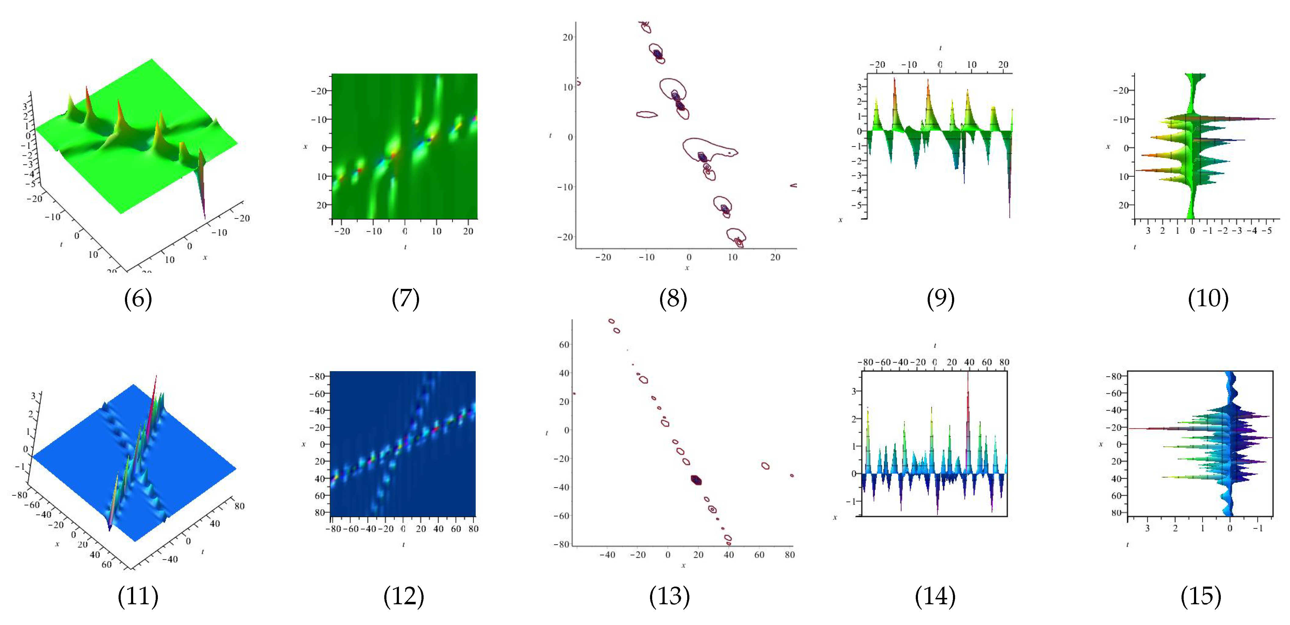
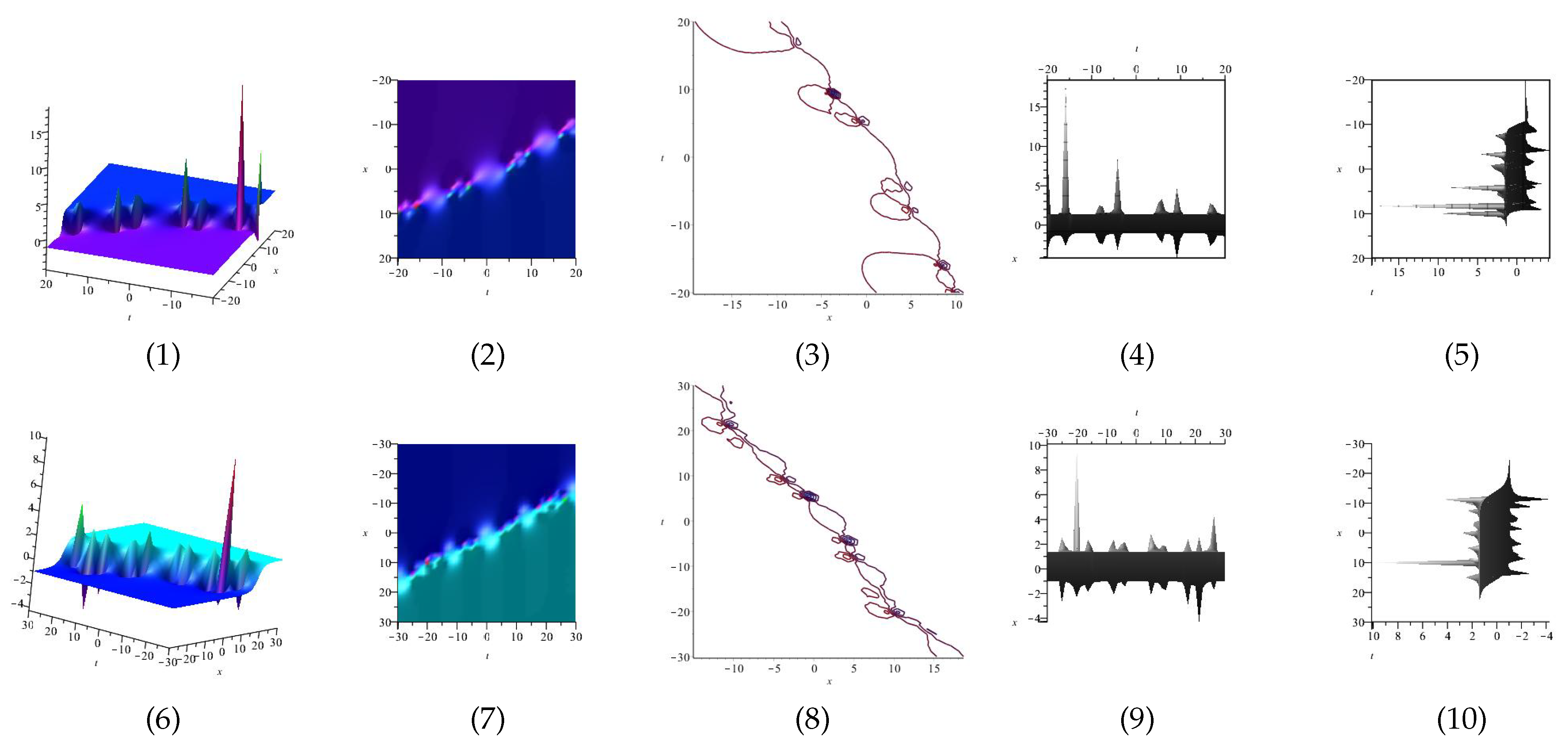
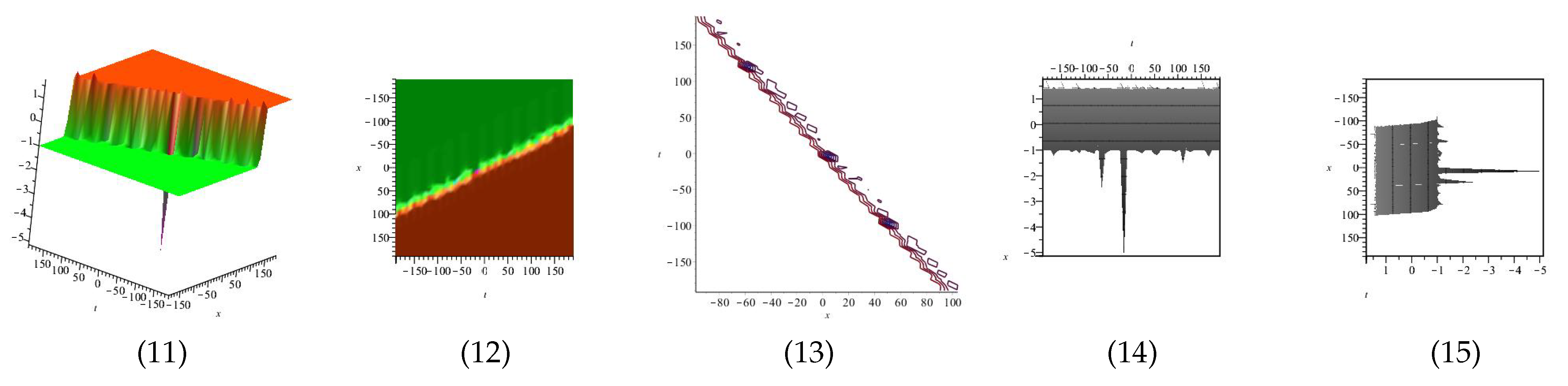
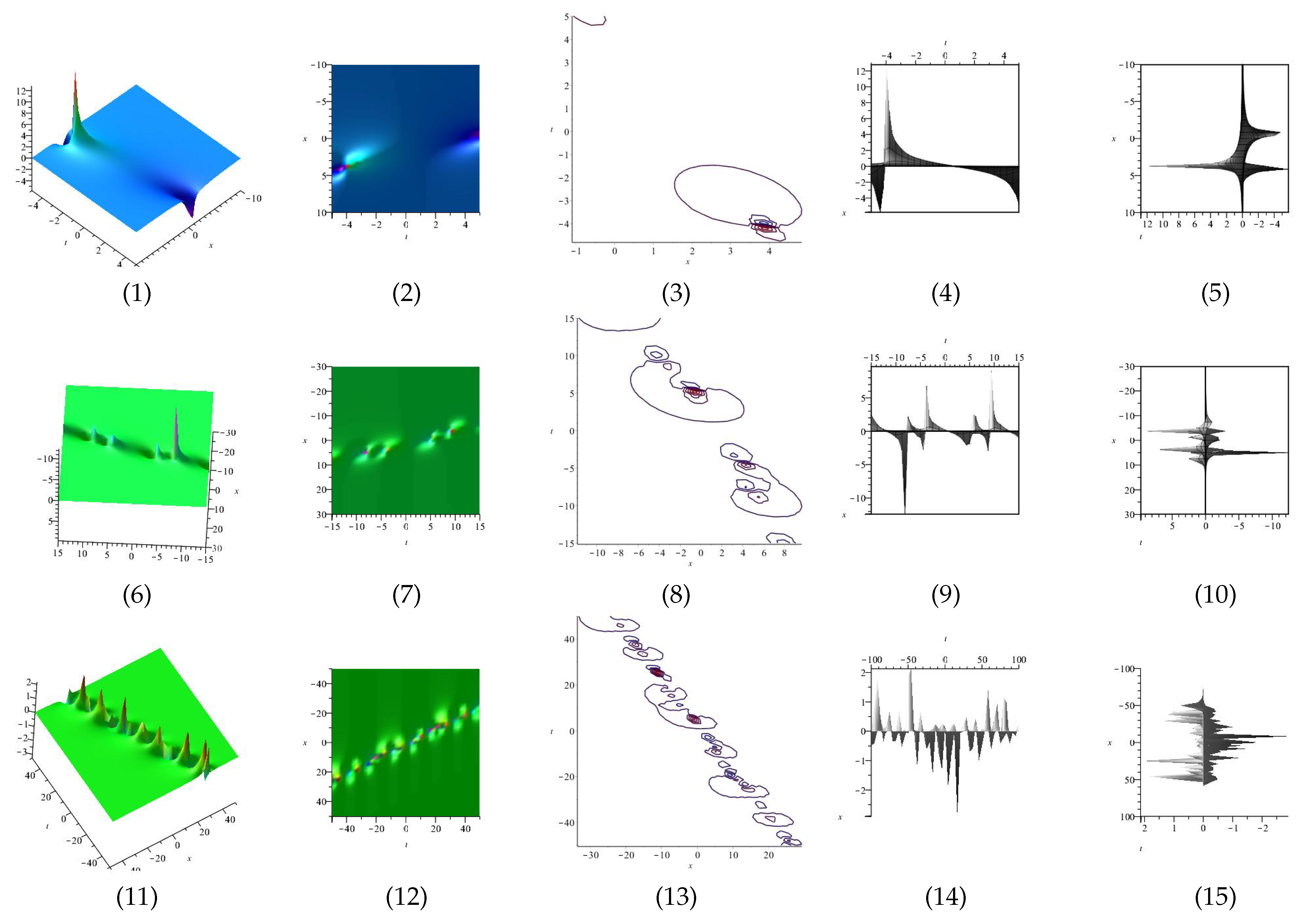
3.2. Application

We apply MEFM to construct the analytical solutions for (3+1)-dimensional nonlinear PDE (1) and spacial cases of (2+1)-dimensional nonlinear PDE (2).

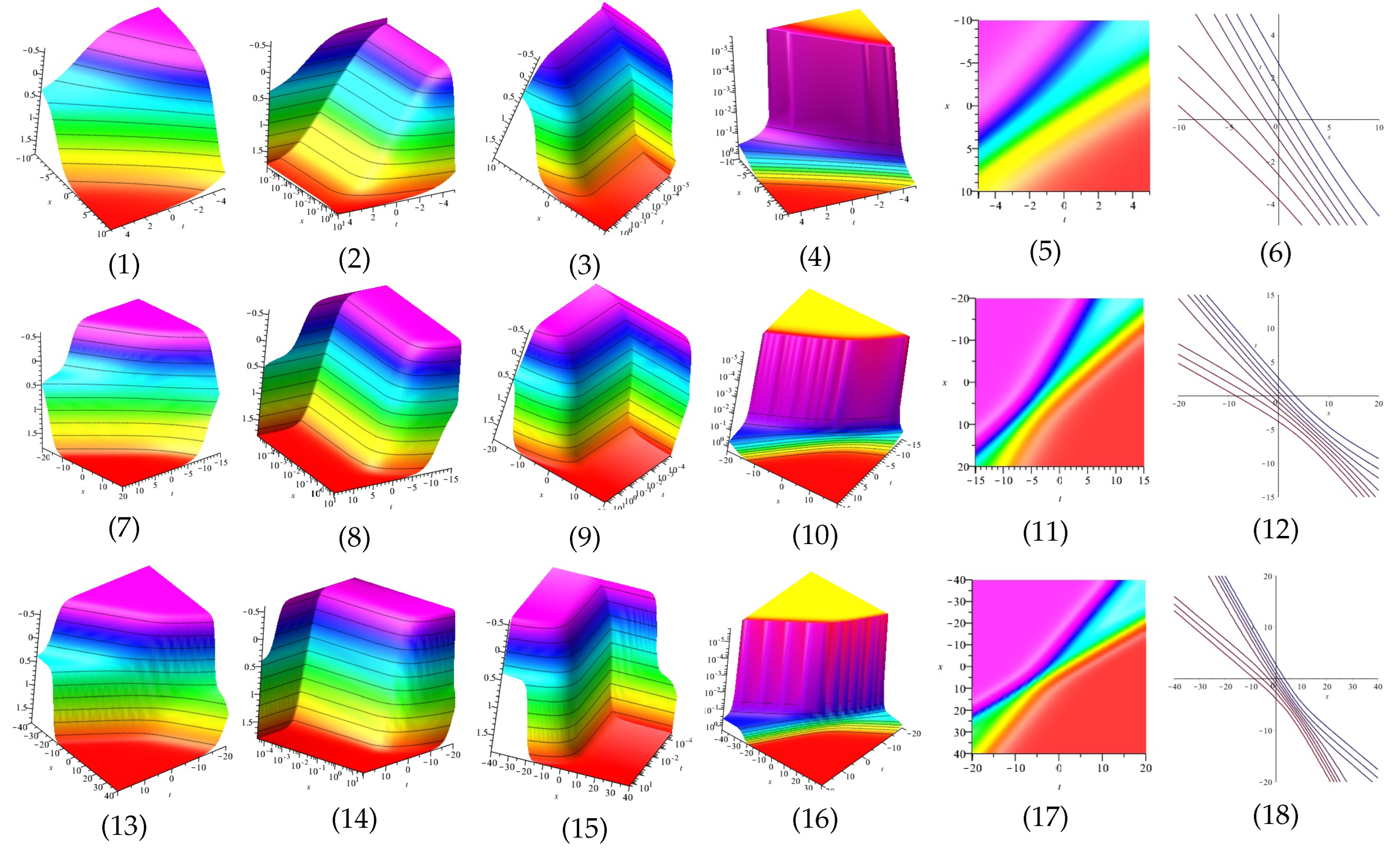
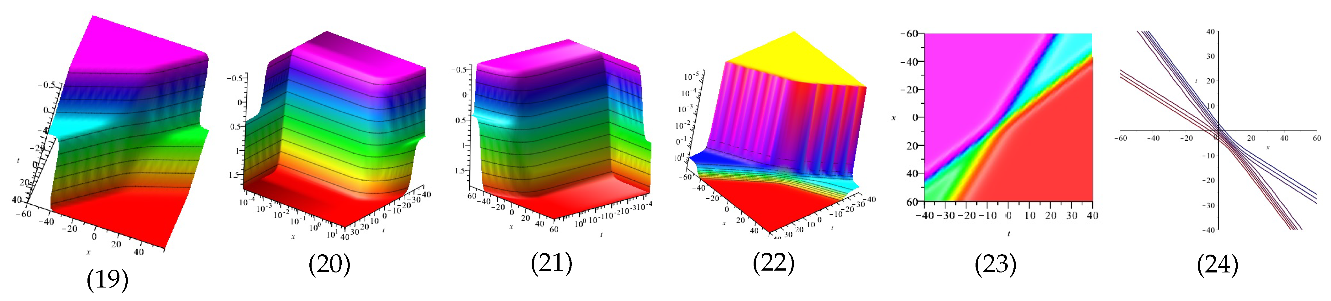
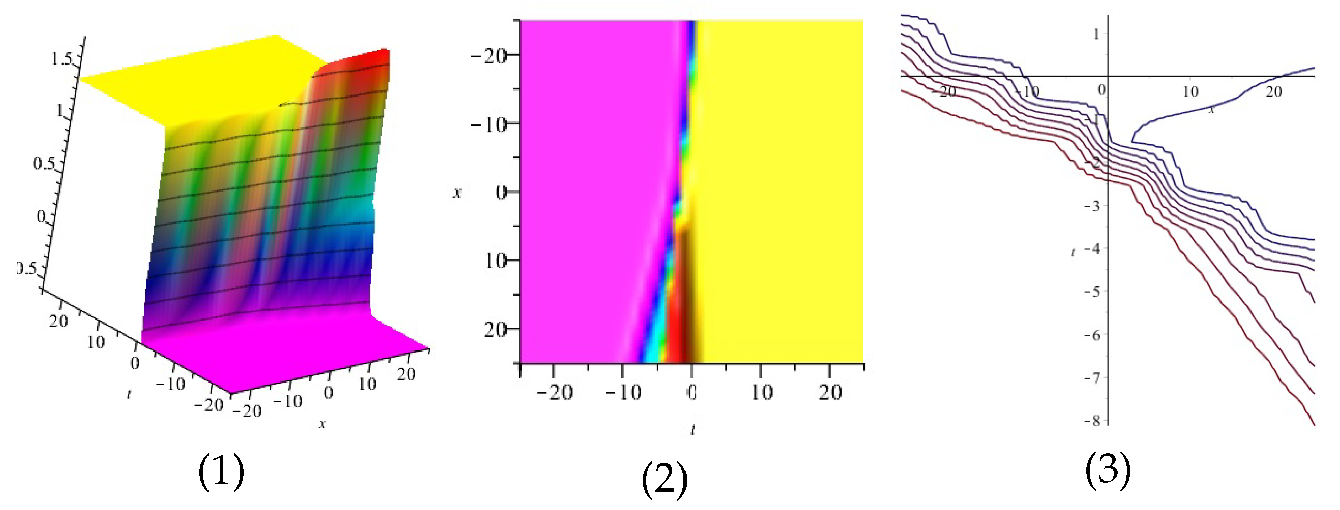
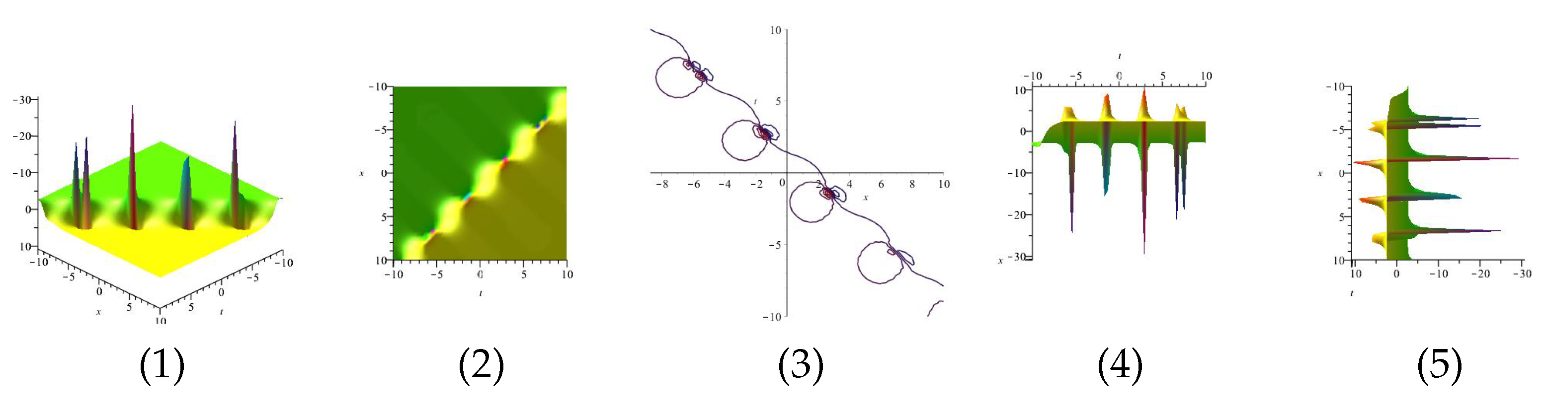
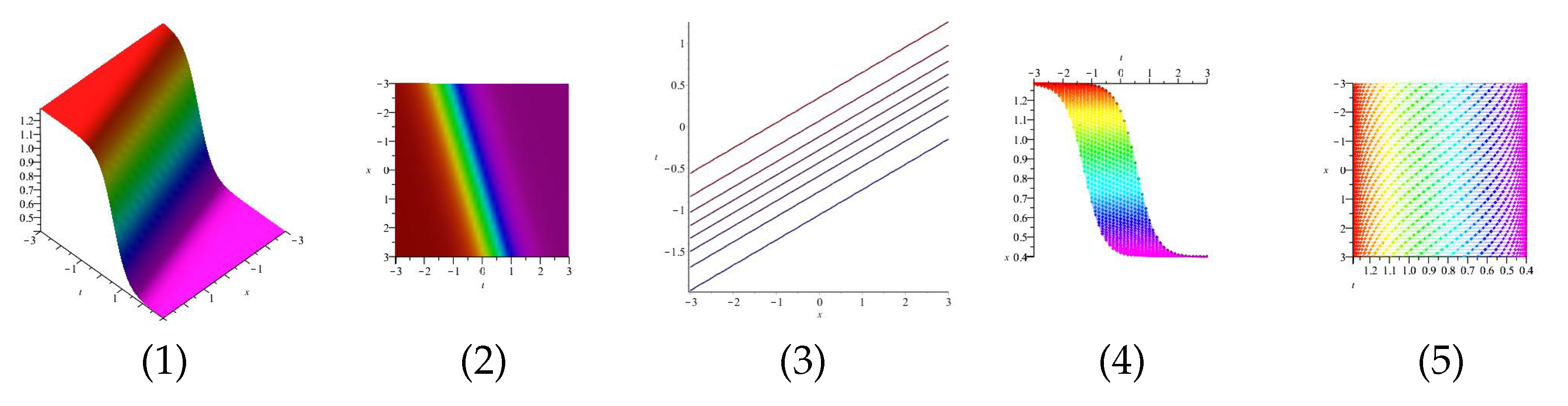
3.2.1. Example 1

Here, we apply MEFM to construct the analytical solutions for (3+1)-dimensional nonlinear PDE presented in (1).

• One wave solutions for (1):

First introduce a variable ${\mu }_1={\mu }_1(x,y,z,t)$ as follows

$$\begin{array}{c}\hfill {\mu }_1={\varpi }_{1}exp(S_{1}x+R_{1}y+A_{1}z-{\omega }_{1}t),\end{array}$$

(32)

where ${\varpi }_1,S_1,R_1,A_1$ and ${\omega }_1$ are constants. Note ${\mu }_1$ has the following linear partial differential relations

$$\begin{array}{c}\hfill {\mu }_{1,x}=S_1{\mu }_1,{\mu }_{1,y}=R_1{\mu }_1,{\mu }_{1,z}=A_1{\mu }_1,{\mu }_{1,t}=-{\omega }_1{\mu }_1.\end{array}$$

(33)

Then, we consider a pair of polynomials of degree one

$$\begin{array}{ccc}& & \mathcal{K}\left({\mu }_1\right)=P_0+P_1{\mu }_1,\hfill \end{array}$$

(34)

$$\begin{array}{ccc}& & \mathcal{H}\left({\mu }_1\right)=Q_0+Q_1{\mu }_1,\hfill \end{array}$$

(35)

where $P_0,P_1,Q_0,$ and $Q_1$ are constants to be determined from (1). Therefore, we have

$$\begin{array}{c}\hfill u(x,t)={\displaystyle \frac{\mathcal{K}\left({\mu }_1\right)}{\mathcal{H}\left({\mu }_1\right)}}={\displaystyle \frac{P_0+P_1{\mu }_1}{Q_0+Q_1{\mu }_1}}.\end{array}$$

(36)

Now, by substituting (36) into (1) and solving the system of algebraic equations, we obtain:

$$\begin{array}{ccc}& & P_1={\displaystyle \frac{Q_1{P}_0}{Q_0}},\hfill \\ & & {\omega }_1:\mathrm{arbitrary},\hfill \end{array}$$

(37)

and

$$\begin{array}{ccc}& & P_1=\mathrm{arbitrary},\hfill \\ & & {\omega }_1:-R_1,\hfill \\ & & A_1=-S_1.\hfill \end{array}$$

(38)

Thus, the one wave solutions can be proposed by

$$\begin{array}{c}\hfill u_{1,1}(x,t)={\displaystyle \frac{P_0+{\displaystyle \frac{Q_1{P}_0}{Q_0}}exp(S_{1}x+R_{1}y+A_{1}z-{\omega }_{1}t)}{Q_0+Q_{1}exp(S_{1}x+R_{1}y+A_{1}z-{\omega }_{1}t)}}\end{array}$$

(39)

and

$$\begin{array}{c}\hfill u_{1,2}(x,t)={\displaystyle \frac{P_0+P_{1}exp(S_{1}x+R_{1}y-S_{1}z+R_{1}t)}{Q_0+Q_{1}exp(S_{1}x+R_{1}y-S_{1}z+R_{1}t)}}.\end{array}$$

(40)

Equation (39) is displayed in Figure 1 for $S_1=Q_1=-0.70,R_1=-P_0=-0.90$, $Q_0=0.40,{\omega }_1=0.5,$ (1), (4) and (7) are three dimensional with $y=z=2.$ Now (2), (5) and (8) exploits the $z-$axis orientation. (3), (6) and (9) are contour plots. Further, Equation (40) is displayed in Figure 2 for $S_1=-3.70,R_1=-2.90,Q_0=0.40,Q_1=-0.70,P_0=0.90,P_1=3,$ (1), (4) and (7) are three dimensional with $y=z=2.$ Now (2), (5) and (8) exploits the $z-$axis orientation. (3), (6) and (9) are contour plots.

• Two wave solutions for (1):

Here, introduce a variable ${\mu }_i={\mu }_i(x,y,z,t),i=1,2,$ as follows

$$\begin{array}{c}\hfill {\mu }_i={\varpi }_{i}exp(S_{i}x+R_{i}y+A_{1}z-{\omega }_{i}t),i=1,2\end{array}$$

(41)

where ${\varpi }_i,S_i,R_i,A_i$ and ${\omega }_i$ are constants. Note ${\mu }_i$ has the following linear partial differential relations

$$\begin{array}{c}\hfill {\mu }_{i,x}=S_i{\mu }_i,{\mu }_{i,y}=R_i,{\mu }_{i,z}=A_i{\mu }_1,{\mu }_{i,t}=-{\omega }_i{\mu }_i,i=1,2.\end{array}$$

(42)

Then, we consider a pair of polynomials of degree two

$$\begin{array}{ccc}& & \mathcal{K}({\mu }_1,{\mu }_2)=2(S_1{\mu }_1+S_2{\mu }_2+P_{12}(S_1+S_2){\mu }_1{\mu }_2),\hfill \end{array}$$

(43)

$$\begin{array}{ccc}& & \mathcal{H}({\mu }_1,{\mu }_2)=1+{\mu }_1+{\mu }_2+P_{12}{\mu }_1{\mu }_2,\hspace{1em}\hspace{1em}\hspace{1em}\hspace{1em}\hspace{1em}\hspace{1em}\hfill \end{array}$$

(44)

where $P_{12}$ is a constant to be determined from (1). Therefore, we have

$$\begin{array}{c}\hfill u(x,t)={\displaystyle \frac{2(S_1{\mu }_1+S_2{\mu }_2+P_{12}(S_1+S_2){\mu }_1{\mu }_2)}{1+{\mu }_1+{\mu }_2+P_{12}{\mu }_1{\mu }_2}}.\end{array}$$

(45)

Now, by substituting (45) into (1) and solving the system of algebraic equations, we obtain:

$$\begin{array}{ccc}\hfill P_{12}& =& 1,\hfill \\ \hfill R_2& =& -S_2,\hfill \\ \hfill A_1& =& -S_1,\hfill \\ \hfill {\omega }_1& =& -R_1,\hfill \\ \hfill {\omega }_2& =& -A_2,\hfill \end{array}$$

and

$$\begin{array}{ccc}\hfill P_{12}& =& 1,\hfill \\ \hfill R_1& =& -S_1,\hfill \\ \hfill A_2& =& -S_2,\hfill \\ \hfill {\omega }_1& =& -A_1,\hfill \\ \hfill {\omega }_2& =& -R_2.\hfill \end{array}$$

By setting the above values in (45), the two wave solutions can be proposed by

$$\begin{array}{ccc}\hfill u_{2,1}(x,t)=& [& 2(S_{1}exp(S_{1}x+R_{1}y-S_{1}z+R_{1}t)+S_{2}exp(S_{2}x-S_{2}y+A_{2}z+A_{2}t)\hfill \\ \hfill & +& (S_1+S_2)exp(S_{1}x+R_{1}y-S_{1}z+R_{1}t)exp(S_{2}x-S_{2}y+A_{2}z+A_{2}t)\left)\right]/\hfill \\ \hfill & [& 1+exp(S_{1}x+R_{1}y-S_{1}z+R_{1}t)+exp(S_{2}x-S_{2}y+A_{2}z+A_{2}t)\hfill \\ \hfill & +& exp(S_{1}x+R_{1}y-S_{1}z+R_{1}t)exp(S_{2}x-S_{2}y+A_{2}z+A_{2}t)],\hfill \end{array}$$

(46)

and

$$\begin{array}{ccc}\hfill u_{2,2}(x,t)=& [& 2(S_{1}exp(S_{1}x-S_{1}y+A_{1}z+A_{1}t)+S_{2}exp(S_{2}x+R_{2}y-S_{2}z+R_{2}t)\hfill \\ \hfill & +& (S_1+S_2)exp(S_{1}x-S_{1}y+A_{1}z+A_{1}t)exp(S_{2}x+R_{2}y-S_{2}z+R_{2}t)\left)\right]/\hfill \\ \hfill & [& 1+exp(S_{1}x-S_{1}y+A_{1}z+A_{1}t)+exp(S_{2}x+R_{2}y-S_{2}z+R_{2}t)\hfill \\ \hfill & +& exp(S_{1}x-S_{1}y+A_{1}z+A_{1}t)exp(S_{2}x+R_{2}y-S_{2}z+R_{2}t)].\hfill \end{array}$$

(47)

Equation (46) is displayed in Figure 3 for $R_1=0.80,A_2=0.40,S_1=0.90,S_2=-7,$ (1), (4) and (7) are three dimensional with $y=3,z=2.$ Now (2), (5) and (8) exploits the $z-$axis orientation. (3), (6) and (9) are contour plots. Further, Equation (47) is displayed in Figure 4 for $R_2=3.90,A_1=5.60,S_1=5.90,S_2=-7.70,$ (1), (4) and (7) are three dimensional with $y=3,z=2.$ Now (2), (5) and (8) exploits the $z-$axis orientation. (3), (6) and (9) are contour plots.

• Three wave solutions for (1):

Here, introduce a variable ${\mu }_i={\mu }_i(x,y,z,t),i=1,2,3,$ as follows

$$\begin{array}{c}\hfill {\mu }_i={\varpi }_{i}exp(S_{i}x+R_{i}y+A_{i}z-{\omega }_{i}t),i=1,2,3\end{array}$$

(48)

where ${\varpi }_i,S_i,R_i,A_I$ and ${\omega }_i$ are constants. Note ${\mu }_i$ has the following linear partial differential relations

$$\begin{array}{c}\hfill {\mu }_{i,x}=S_i{\mu }_i,{\mu }_{i,y}=R_i{\mu }_1,{\mu }_{i,z}=A_i{\mu }_1,{\mu }_{i,t}=-{\omega }_i{\mu }_i,i=1,2,3.\end{array}$$

(49)

Then, we consider a pair of polynomials of degree three

$$\begin{array}{ccc}\hfill \mathcal{K}({\mu }_1,{\mu }_2,{\mu }_3)& =& 2(S_1{\mu }_1+S_2{\mu }_2+S_3{\mu }_3+P_{12}(S_1+S_2){\mu }_1{\mu }_2+P_{13}(S_1+S_3){\mu }_1{\mu }_3\hfill \\ & & +P_{23}(S_2+S_3){\mu }_2{\mu }_3+P_{12}{P}_{13}{P}_{23}(S_1+S_2+S_3){\mu }_1{\mu }_2{\mu }_3),\hfill \end{array}$$

and

$$\begin{array}{ccc}\hfill \mathcal{H}({\mu }_1,{\mu }_2,{\mu }_3)& =& 1+{\mu }_1+{\mu }_2+{\mu }_3+P_{12}{\mu }_1{\mu }_2+P_{13}{\mu }_1{\mu }_3+P_{23}{\mu }_2{\mu }_3\hfill \\ & & +P_{12}{P}_{13}{P}_{23}{\mu }_1{\mu }_2{\mu }_3,\hfill \end{array}$$

where $P_{12},P_{13},$ and $P_{23}$ are constants to be determined from (1). Therefore, we have

$$\begin{array}{ccc}\hfill u(x,t)=& [& 2(S_1{\mu }_1+S_2{\mu }_2+S_3{\mu }_3+P_{12}(S_1+S_2){\mu }_1{\mu }_2+P_{13}(S_1+S_3){\mu }_1{\mu }_3\hfill \\ \hfill & +& P_{23}(S_2+S_3){\mu }_2{\mu }_3+P_{12}{P}_{13}{P}_{23}(S_1+S_2+S_3){\mu }_1{\mu }_2{\mu }_3\left)\right]/\hfill \\ \hfill & [& 1+{\mu }_1+{\mu }_2+{\mu }_3+P_{12}{\mu }_1{\mu }_2+P_{13}{\mu }_1{\mu }_3+P_{23}{\mu }_2{\mu }_3+P_{12}{P}_{13}{P}_{23}{\mu }_1{\mu }_2{\mu }_3].\hfill \end{array}$$

(50)

Now, by substituting (50) into (1) and solving the system of algebraic equations, we obtain:

$$\begin{array}{ccc}\hfill P_{12}& =& 1,\hfill \\ \hfill P_{13}& =& 0,\hfill \\ \hfill P_{23}& =& 1,\hfill \\ \hfill A_1& =& -S_1,\hfill \\ \hfill A_3& =& -S_3,\hfill \\ \hfill R_2& =& -S_2,\hfill \\ \hfill {\omega }_1& =& -R_1,\hfill \\ \hfill {\omega }_2& =& -A_2,\hfill \\ \hfill {\omega }_3& =& -R_3,\hfill \end{array}$$

$$\begin{array}{ccc}\hfill P_{12}& =& 0,\hfill \\ \hfill P_{13}& =& 1,\hfill \\ \hfill P_{23}& =& 1,\hfill \\ \hfill A_1& =& -S_1,\hfill \\ \hfill A_2& =& -S_2,\hfill \\ \hfill R_3& =& -S_3,\hfill \\ \hfill {\omega }_1& =& -R_1,\hfill \\ \hfill {\omega }_2& =& -R_2,\hfill \\ \hfill {\omega }_3& =& -A_3,\hfill \end{array}$$

(51)

$$\begin{array}{ccc}\hfill P_{12}& =& 0,\hfill \\ \hfill P_{13}& =& 1,\hfill \\ \hfill P_{23}& =& 1,\hfill \\ \hfill R_1& =& -S_1,\hfill \\ \hfill R_2& =& -S_2,\hfill \\ \hfill A_3& =& -S_3,\hfill \\ \hfill {\omega }_1& =& -A_1,\hfill \\ \hfill {\omega }_2& =& -A_2,\hfill \\ \hfill {\omega }_3& =& -R_3,\hfill \end{array}$$

(52)

$$\begin{array}{ccc}\hfill P_{12}& =& \mathrm{arbitrary},\hfill \\ \hfill P_{13}& =& 0,\hfill \\ \hfill P_{23}& =& 0,\hfill \\ \hfill R_1& =& -S_1,\hfill \\ \hfill R_2& =& -S_2,\hfill \\ \hfill R_3& =& -S_3,\hfill \\ \hfill {\omega }_1& =& -A_1,\hfill \\ \hfill {\omega }_2& =& -A_2,\hfill \\ \hfill {\omega }_3& =& -A_3.\hfill \end{array}$$

(53)

Thus, the three wave solutions can be proposed by

$$\begin{array}{ccc}\hfill u_{3,1}(x,t)=& [& 2(S_{1}exp(S_{1}x+R_{1}y-S_{1}z+R_{1}t)\hfill \\ \hfill & +& S_{2}exp(S_{2}x-S_{2}y+A_{2}z+A_{2}t)+S_{3}exp(S_{3}x+R_{3}y-S_{3}z+R_{3}t)\hfill \\ \hfill & +& (S_1+S_2)exp(S_{1}x+R_{1}y-A_{1}z+R_{1}t)exp(S_{2}x-S_{2}y+A_{2}z+A_{2}t)\hfill \\ \hfill & +& (S_2+S_3)exp(S_{2}x-S_{2}y+A_{2}z+A_{2}t)exp(S_{3}x+R_{3}y-S_{3}z+R_{3}t)\left)\right]/\hfill \\ \hfill & [& 1+exp(S_{1}x+R_{1}y-A_{1}z+R_{1}t)+exp(S_{2}x-S_{2}y+A_{2}z+A_{2}t)\hfill \\ \hfill & +& exp(S_{3}x+R_{3}y-S_{3}z+R_{3}t)+exp(S_{1}x+R_{1}y-S_{1}z+R_{1}t)\hfill \\ \hfill & & exp(S_{2}x-S_{2}y+A_{2}z+A_{2}t)+exp(S_{2}x-S_{2}y+A_{2}z+A_{2}t)\hfill \\ \hfill & & exp(S_{3}x+R_{3}y-S_{3}z+R_{3}t)],\hfill \end{array}$$

(54)

and also, by inserting (51), (52), and (53) in (50), we obtain $u_{3,2}(x,t),u_{3,3}(x,t)$ and $u_{3,4}(x,t),$ respectively.

Equation (54) is displayed in Figure 5 for $R_1=0.50,R_3=-0.70,S_1=0.20,$ $S_2=0.70,$ $S_3=-0.30,A_1=0.80,$ and equation $u_{3,2}$ is displayed in Figure 6 for $R_1=-0.50,$ $R_2=-0.70,$ $S_1=0.20,S_2=0.70,S_3=-0.30,A_3=0.80,$ in different domains. Equation $u_{3,3}$ is displayed in Figure 7 for $R_3=-2.70,A_1=-2.70,A_2=2.80,S_1=2.20,$ $S_2=2.70,$ $S_3=-2.30,$ (1), (4) and (7) are three dimensional with $y=z=2.$ Now (2), (5) and (8) exploit the $z-$axis orientation. (3), (6) and (9) are contour plots. Further, equation $u_{3,4}$ is displayed in Figure 8 for $P_{12}=3.50,A_1=-3,A_2=-5,A_3=7,S_1=0.20,S_2=0.70,$ $S_3=-0.30,$ (1), (4) and (7) are three dimensional with $y=z=2.$ Now (2), (5) and (8) exploit the $z-$axis orientation. (3), (6) and (9) are contour plots.

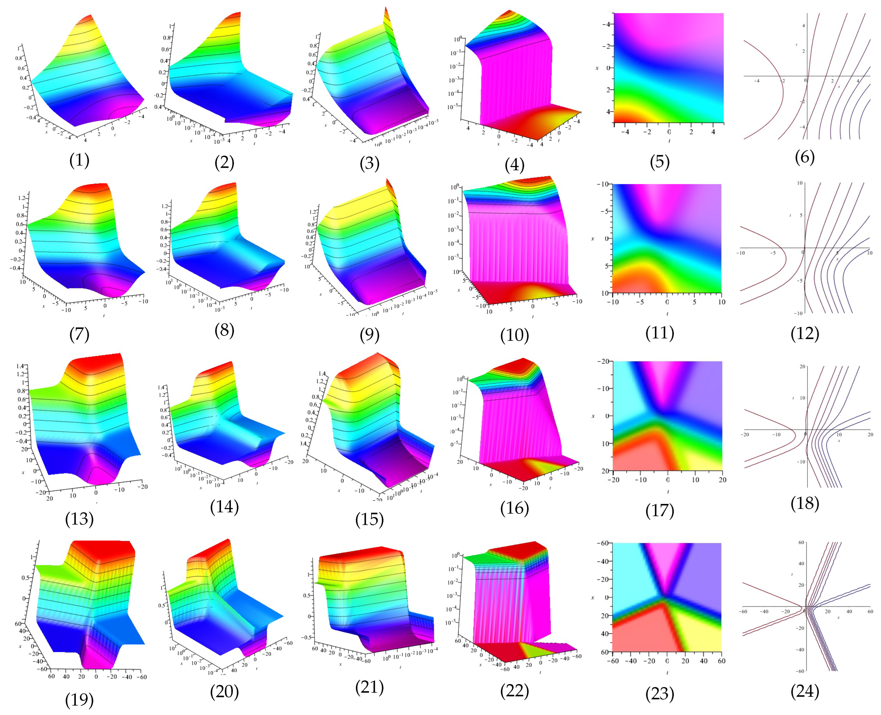
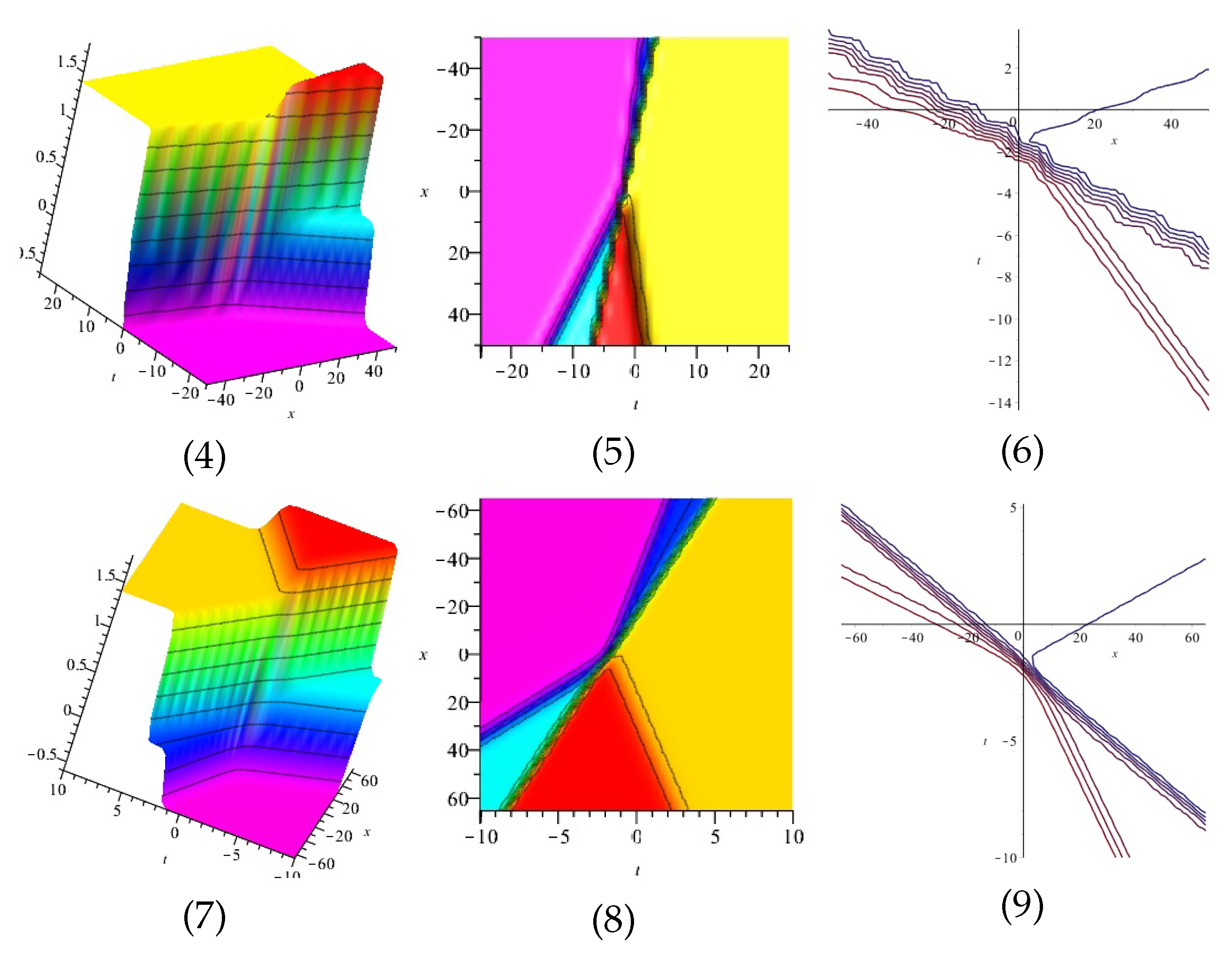
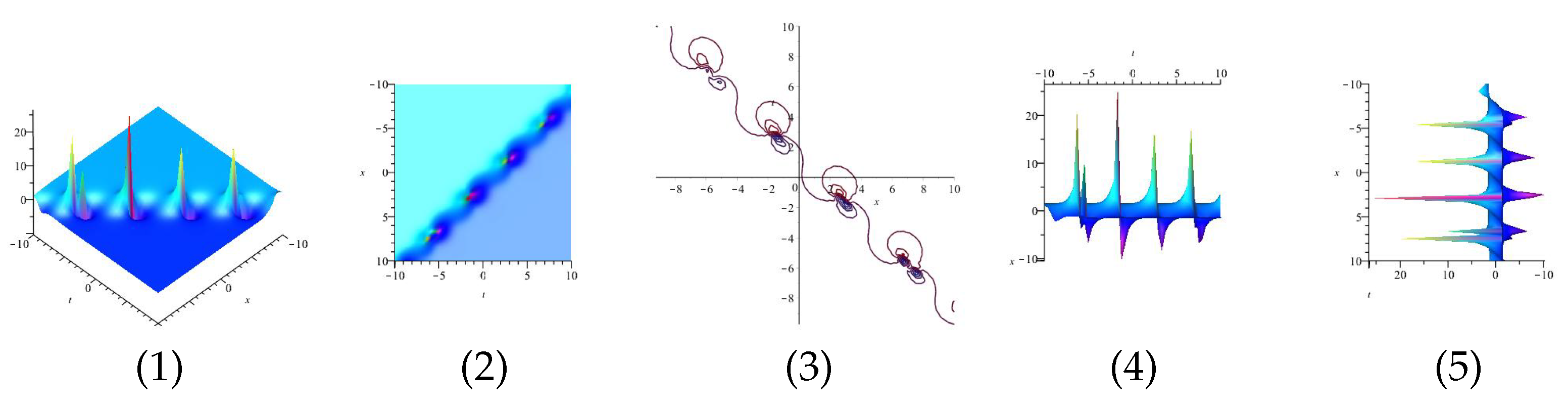
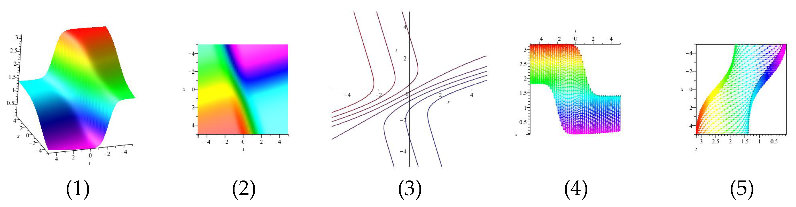
3.2.2. Example 2

Here, we apply MEFM to construct the new exact solutions for the (2+1)-dimensional Equation (3).

• One wave solutions for (3):

Firstly, introduce a variable ${\mu }_1={\mu }_1(x,y,t)$ as follows

$$\begin{array}{c}\hfill {\mu }_1={\varpi }_{1}exp(S_{1}x+R_{1}y-{\omega }_{1}t),\end{array}$$

(55)

where ${\varpi }_1,S_1,R_1$ and ${\omega }_1$ are constants. Obviously, ${\mu }_1$ has the following linear partial differential relations

$$\begin{array}{c}\hfill {\mu }_{1,x}=S_1{\mu }_1,{\mu }_{1,y}=R_1{\mu }_1,{\mu }_{1,t}=-{\omega }_1{\mu }_1.\end{array}$$

(56)

Therefore, we consider a pair of polynomials of degree one

$$\begin{array}{ccc}& & \mathcal{K}\left({\mu }_1\right)=P_0+P_1{\mu }_1,\hfill \end{array}$$

(57)

$$\begin{array}{ccc}& & \mathcal{H}\left({\mu }_1\right)=Q_0+Q_1{\mu }_1,\hfill \end{array}$$

(58)

where $P_0,P_1,Q_0,$ and $Q_1$ are constants to be determined from (1). Therefore, we have

$$\begin{array}{c}\hfill u(x,t)={\displaystyle \frac{\mathcal{K}\left({\mu }_1\right)}{\mathcal{H}\left({\mu }_1\right)}}={\displaystyle \frac{P_0+P_1{\mu }_1}{Q_0+Q_1{\mu }_1}}.\end{array}$$

(59)

Now, by substituting (59) into (3) and solving the system of algebraic equations, we obtain:

$$\begin{array}{ccc}& & P_1:\mathrm{arbitrary},\hfill \\ & & {\omega }_1=(1.500+0.866i)R_1,\hfill \\ & & S_1=-{\displaystyle \frac{R_1(1.500+0.866i)R_1-1.500+0.866i)}{-R_1+(1.500+0.866i)R_1-1}}.\hfill \end{array}$$

(60)

Thus, the one wave solutions can be proposed by

$$\begin{array}{ccc}\hfill & & u_1(x,t)=\left[P_0+P_{1}exp(-{\displaystyle \frac{R_1(1.500+0.866i)R_1-1.500+0.866i)}{-R_1+(1.500+0.866i)R_1-1}}x+R_{1}y-(1.500+0.866i)R_1)t)\right]/\hfill \\ & & \left[Q_0+Q_{1}exp(-{\displaystyle \frac{R_1(1.500+0.866i)R_1-1.500+0.866i)}{-R_1+(1.500+0.866i)R_1-1}}x+R_{1}y-(1.500+0.866i)R_1)t)\right]\hfill \end{array}$$

(61)

The real and imaginary part of Equation (61) are displayed in Figure 9 and Figure 10 for $P_1=0.20,P_0=0.90,Q_0=0.70,Q_1=0.50,R_1=-0.90.$ (1) is three dimensional with $y=z=2.$ (2), (4) and (5) exploit $z-$axis, $x-$axis, $y-$axis orientation, respectively, and (3) is contour plot.

• Two wave solutions for (3):

Here, introduce a variable ${\mu }_i={\mu }_i(x,y,t),i=1,2,$ as follows

$$\begin{array}{c}\hfill {\mu }_i={\varpi }_{i}exp(S_{i}x+R_{i}y-{\omega }_{i}t),i=1,2\end{array}$$

(62)

where ${\varpi }_i,S_i,R_i,$ and ${\omega }_i$ are constants. Obviously, ${\mu }_i$ has the following linear partial differential relations

$$\begin{array}{c}\hfill {\mu }_{i,x}=S_i{\mu }_i,{\mu }_{i,y}=R_i,{\mu }_{i,t}=-{\omega }_i{\mu }_i,i=1,2.\end{array}$$

(63)

Then, we consider a pair of polynomials of degree two

$$\begin{array}{ccc}& & \mathcal{K}({\mu }_1,{\mu }_2)=2(S_1{\mu }_1+S_2{\mu }_2+P_{12}(S_1+S_2){\mu }_1{\mu }_2),\hfill \end{array}$$

(64)

$$\begin{array}{ccc}& & \mathcal{H}({\mu }_1,{\mu }_2)=1+{\mu }_1+{\mu }_2+P_{12}{\mu }_1{\mu }_2,\hspace{1em}\hspace{1em}\hspace{1em}\hspace{1em}\hspace{1em}\hspace{1em}\hfill \end{array}$$

(65)

where $P_{12}$ is a constant to be determined from (1). Therefore, we have

$$\begin{array}{c}\hfill u(x,t)={\displaystyle \frac{2(S_1{\mu }_1+S_2{\mu }_2+P_{12}(S_1+S_2){\mu }_1{\mu }_2)}{1+{\mu }_1+{\mu }_2+P_{12}{\mu }_1{\mu }_2}}.\end{array}$$

(66)

Now, by substituting (66) into (3) and solving the system of algebraic equations, we obtain:

$$\begin{array}{ccc}& & P_{12}=1,\hfill \\ & & S_1=(-{\displaystyle \frac{3}{2}}+{\displaystyle \frac{1}{2}}\sqrt{3}i)R_1,\hfill \\ & & S_2=(-{\displaystyle \frac{3}{2}}+{\displaystyle \frac{1}{2}}\sqrt{3}i)R_2,\hfill \\ & & {\omega }_1={\displaystyle \frac{R_1((-{\displaystyle \frac{3}{2}}+{\displaystyle \frac{1}{2}}\sqrt{3}i)R_1+{\displaystyle \frac{3}{2}}+{\displaystyle \frac{1}{2}}\sqrt{3}i)}{(-{\displaystyle \frac{3}{2}}+{\displaystyle \frac{1}{2}}\sqrt{3}i)R_1+R_1+1}},\hfill \\ & & {\omega }_2={\displaystyle \frac{R_2((-{\displaystyle \frac{3}{2}}+{\displaystyle \frac{1}{2}}\sqrt{3}i)R_2+{\displaystyle \frac{3}{2}}+{\displaystyle \frac{1}{2}}\sqrt{3}i)}{(-{\displaystyle \frac{3}{2}}+{\displaystyle \frac{1}{2}}\sqrt{3}i)R_2+R_2+1}}.\hfill \end{array}$$

By setting above values in (66), the two wave solutions can be proposed by $u_2(x,t).$

The real and imaginary part of equation $u_2(x,t)$ are displayed in Figure 11 and Figure 12 for $R_1=0.90,R_2=0.80.$ (1) is three dimensional with $y=z=2.$ (2), (4) and (5) exploit $z-$axis, $x-$axis, $y-$axis orientation, respectively, and (3) is contour plot.

• Three wave solutions for (3):

Here, introduce a variable ${\mu }_i={\mu }_i(x,y,t),i=1,2,3,$ as follows

$$\begin{array}{c}\hfill {\mu }_i={\varpi }_{i}exp(S_{i}x+R_{i}y-{\omega }_{i}t),i=1,2,3\end{array}$$

(67)

where ${\varpi }_i,S_i,R_i,$ and ${\omega }_i$ are constants. Obviously, ${\mu }_i$ has the following linear partial differential relations

$$\begin{array}{c}\hfill {\mu }_{i,x}=S_i{\mu }_i,{\mu }_{i,y}=R_i{\mu }_1,{\mu }_{i,t}=-{\omega }_i{\mu }_i,i=1,2,3.\end{array}$$

(68)

Then, we consider a pair of polynomials of degree three

$$\begin{array}{ccc}& & \mathcal{K}({\mu }_1,{\mu }_2,{\mu }_3)=2(S_1{\mu }_1+S_2{\mu }_2+S_3{\mu }_3+P_{12}(S_1+S_2){\mu }_1{\mu }_2\hfill \\ & & +P_{13}(S_1+S_3){\mu }_1{\mu }_3+P_{23}(S_2+S_3){\mu }_2{\mu }_3+P_{12}{P}_{13}{P}_{23}(S_1+S_2+S_3){\mu }_1{\mu }_2{\mu }_3),\hfill \end{array}$$

and

$$\begin{array}{ccc}& & \mathcal{H}({\mu }_1,{\mu }_2,{\mu }_3)=1+{\mu }_1+{\mu }_2+{\mu }_3+P_{12}{\mu }_1{\mu }_2+P_{13}{\mu }_1{\mu }_3+P_{23}{\mu }_2{\mu }_3\hfill \\ & & +P_{12}{P}_{13}{P}_{23}{\mu }_1{\mu }_2{\mu }_3,\hfill \end{array}$$

where $P_{12},P_{13},$ and $P_{23}$ are constants to be determined from (1). Therefore, we have

$$\begin{array}{ccc}\hfill & & u(x,t)=\left[2\right(S_1{\mu }_1+S_2{\mu }_2+S_3{\mu }_3+P_{12}(S_1+S_2){\mu }_1{\mu }_2\hfill \\ & & +P_{13}(S_1+S_3){\mu }_1{\mu }_3+P_{23}(S_2+S_3){\mu }_2{\mu }_3+P_{12}{P}_{13}{P}_{23}(S_1+S_2+S_3){\mu }_1{\mu }_2{\mu }_3\left)\right]/\hfill \\ & & \left[1+{\mu }_1+{\mu }_2+{\mu }_3+P_{12}{\mu }_1{\mu }_2+P_{13}{\mu }_1{\mu }_3+P_{23}{\mu }_2{\mu }_3+P_{12}{P}_{13}{P}_{23}{\mu }_1{\mu }_2{\mu }_3\right].\hfill \end{array}$$

(69)

Now, by substituting (69) into (3) and solving the system of algebraic equations, we obtain:

$$\begin{array}{ccc}& & P_{12}=1,\hfill \\ & & P_{13}=1,\hfill \\ & & P_{23}=1,\hfill \\ & & R_1=-{\displaystyle \frac{S_1((-0.500+0.866i)S_1-1.500+0.866i))}{-S_1+(-0.500+0.866i)S_1-3}},\hfill \\ & & R_2=-{\displaystyle \frac{S_2((-0.500+0.866i)S_2-1.500+0.866i))}{-S_2+(-0.500+0.866i)S_2-3}},\hfill \\ & & R_3=-{\displaystyle \frac{S_3((-0.500+0.866i)S_3-1.500+0.866i))}{-S_3+(-0.500+0.866i)S_3-3}},\hfill \\ & & {\omega }_1=(-0.500+0.866i)S_1,\hfill \\ & & {\omega }_2=(-0.500+0.866i)S_2,\hfill \\ & & {\omega }_3=(-0.500+0.866i)S_3,\hfill \end{array}$$

and

$$\begin{array}{ccc}& & P_{12}=0,\hfill \\ & & P_{13}:\mathrm{arbitrary},\hfill \\ & & P_{23}=0,\hfill \\ & & R_1=(-0.500+0.288i)S_1,\hfill \\ & & R_2=-{\displaystyle \frac{S_2((-0.500+0.866i)S_2-1.500+0.866i))}{-S_2+(-0.500+0.866i)S_2-3}},\hfill \\ & & R_3=(-0.500+0.288i)S_3,\hfill \\ & & {\omega }_1={\displaystyle \frac{S_1((-1.500+0.866i-S_1)}{(0.500+0.866i)S_1+1.500+0.866i+S_1}},\hfill \\ & & {\omega }_2=(-0.500+0.866i)S_2,\hfill \\ & & {\omega }_3={\displaystyle \frac{S_3((-1.500+0.866i-S_3)}{(0.500+0.866i)S_3+1.500+0.866i+S_3}}.\hfill \end{array}$$

By inserting above values in (69), we obtain $u_{3,1}(x,t),u_{3,2}(x,t),$ respectively.

The real and imaginary part of equation $u_{3,1}(x,t)$ and $u_{3,2}(x,t)$ are displayed in Figure 13, Figure 14, Figure 15 and Figure 16 for $S_1=0.20,S_2=0.70,S_3=-0.50.$ (1) is three dimensional with $y=z=2.$ (2), (4) and (5) exploit $z-$axis, $x-$axis, $y-$axis orientation, respectively, and (3) is contour plot, in different domains.

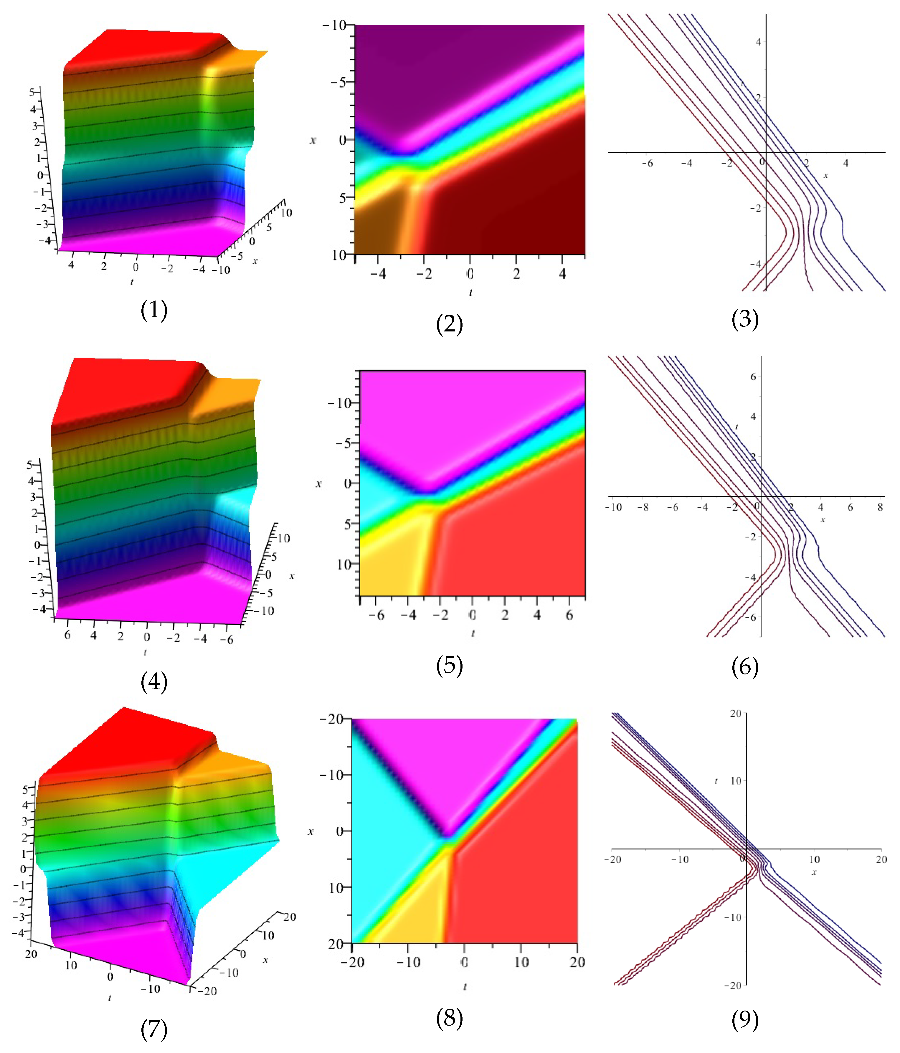
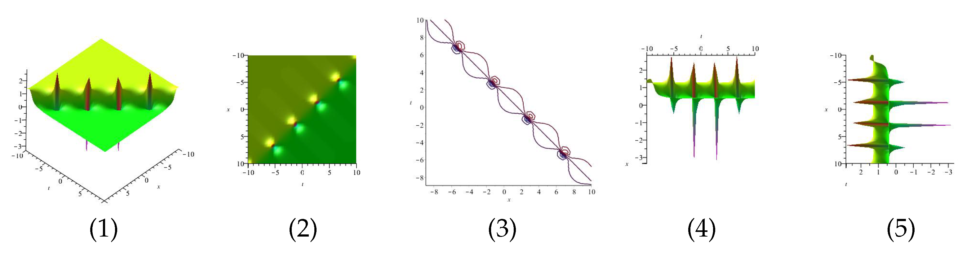
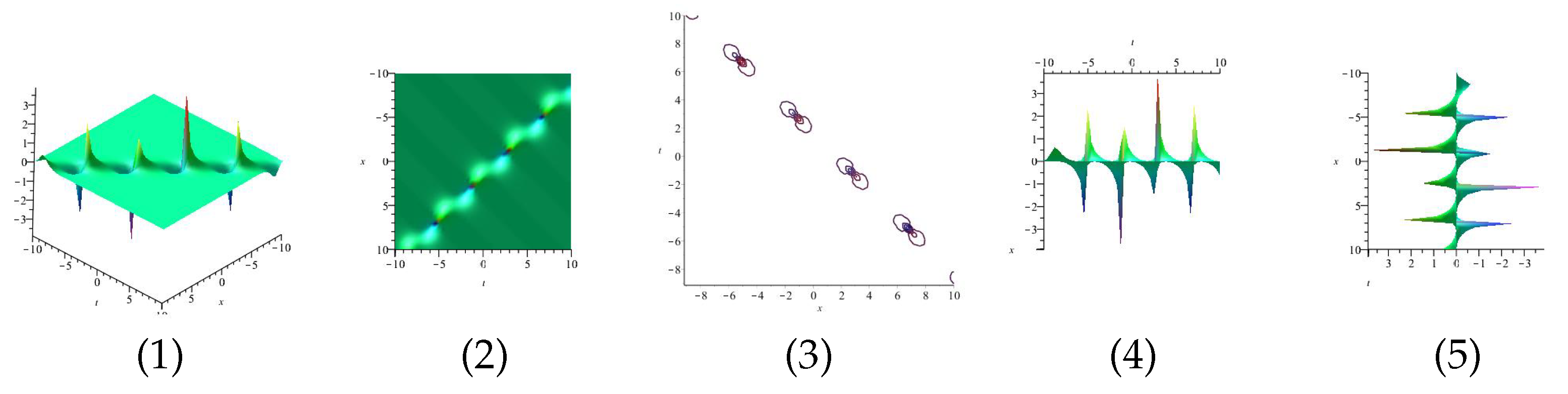
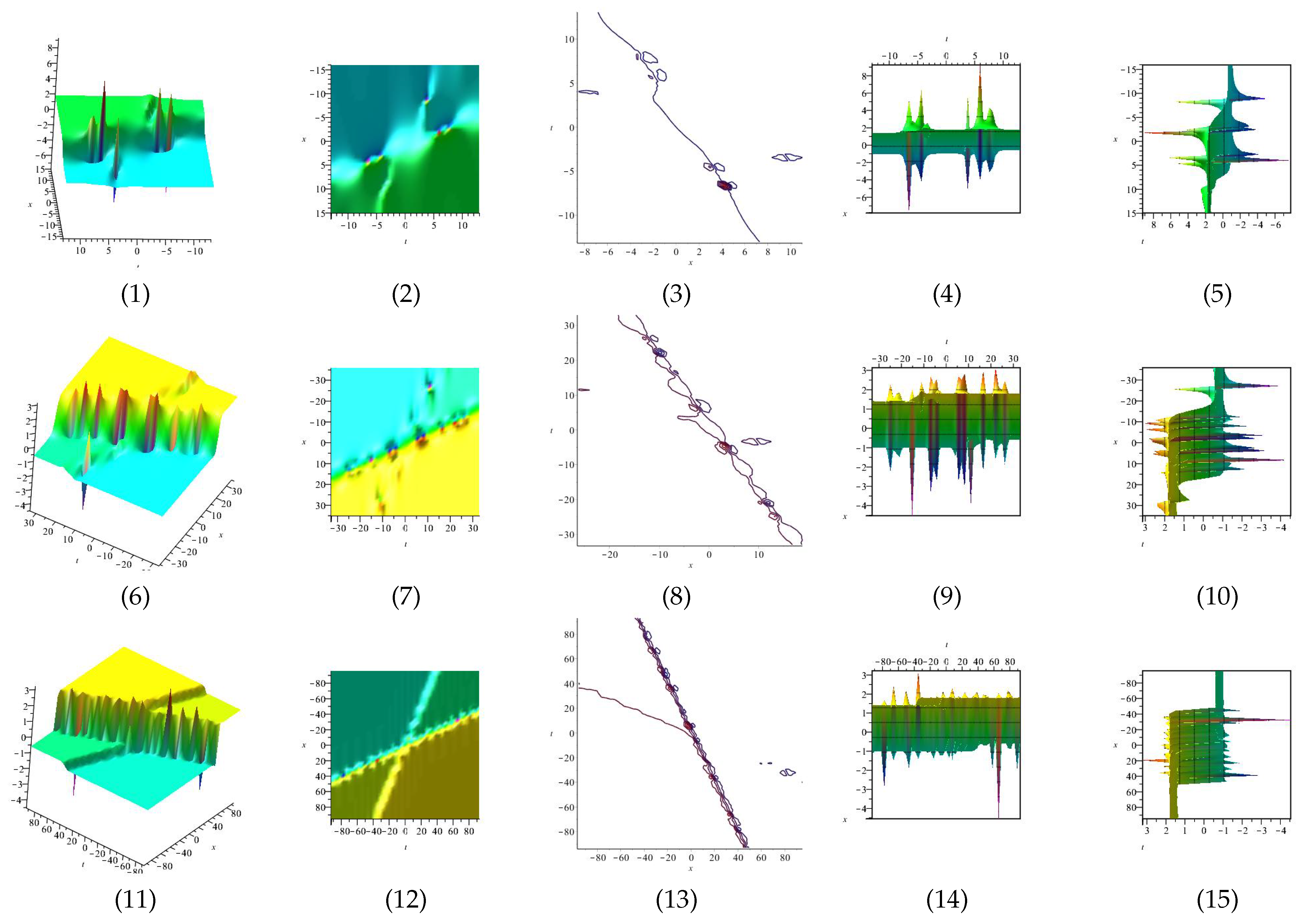
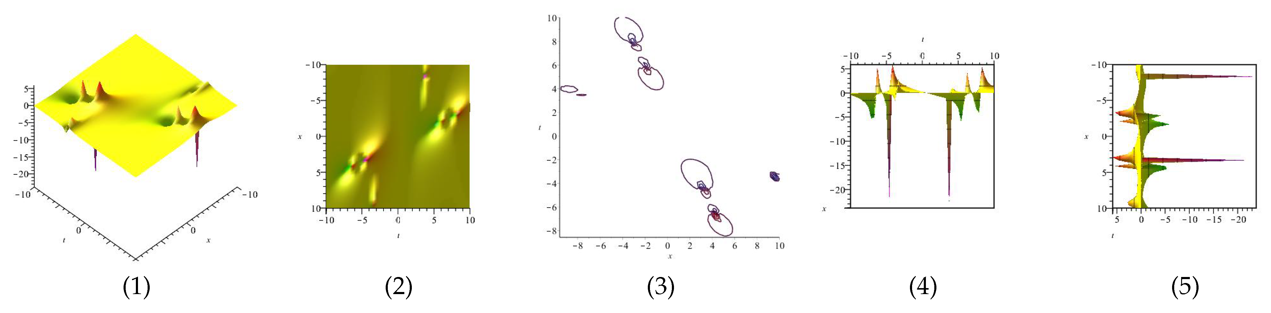
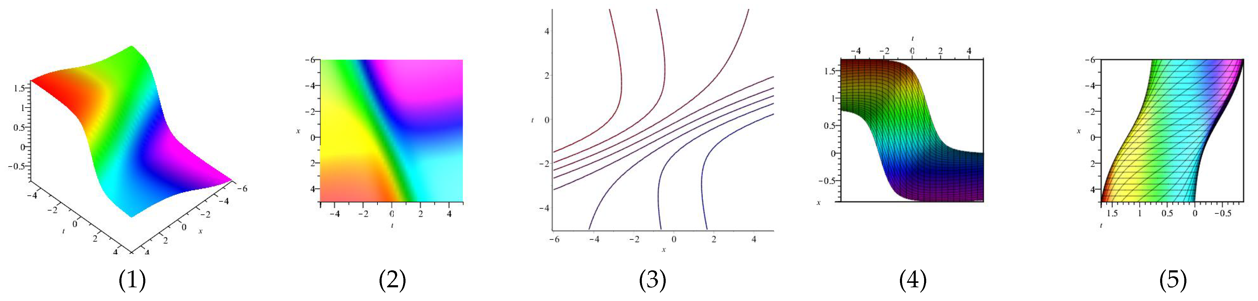
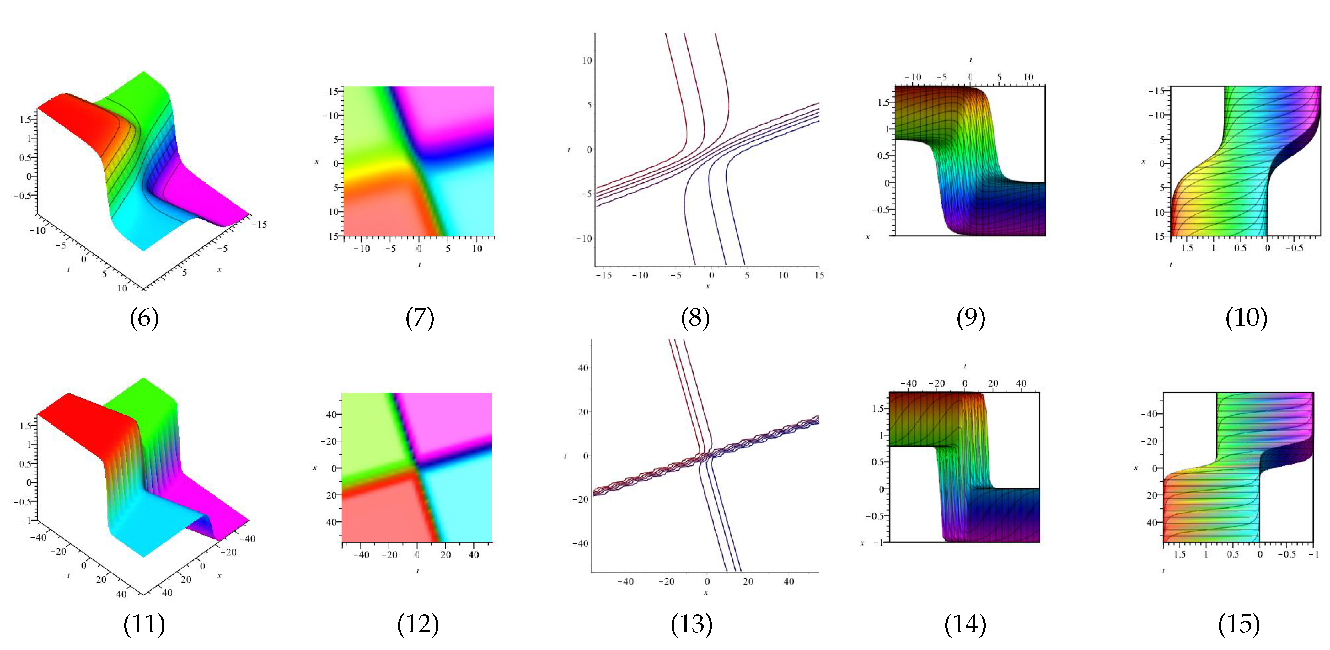
3.2.3. Example 3

Here, we apply MEFM to construct the new exact solutions for the (2+1)-dimensional equation (4).

• One wave solutions for (4):

$$\begin{array}{ccc}& & P_1:\mathrm{arbitrary},\hfill \\ & & R_1=-{\displaystyle \frac{S_1(3.302S_1-2.302)}{4.302S_1-3}},\hfill \\ & & {\omega }_1=3.302S_1.\hfill \end{array}$$

According to the above values, we obtain $u_1^{\prime }(x,t).$, respectively.

Equation $u_1^{\prime }(x,t)$ is displayed in Figure 17 for $S_1=-0.90,P_0=0.90,P_1=0.20,Q_0=0.70,Q_1=0.50.$ (1) is three dimensional with $y=z=2.$ (2), (4) and (5) exploit $z-$axis, $x-$axis, $y-$axis orientation, respectively, and (3) is contour plot, in different domains.

• Two wave solutions for (4):

$$\begin{array}{ccc}& & P_{12}=1,\hfill \\ & & R_1=-{\displaystyle \frac{S_1(({\displaystyle \frac{3}{2}}+{\displaystyle \frac{1}{2}}\sqrt{13})S_1-{\displaystyle \frac{1}{2}}-{\displaystyle \frac{1}{2}}\sqrt{13})}{S_1+({\displaystyle \frac{3}{2}}+{\displaystyle \frac{1}{2}}\sqrt{13})S_1-3}},\hfill \\ & & R_2=(-{\displaystyle \frac{1}{6}}+{\displaystyle \frac{1}{6}}\sqrt{13})S_2,\hfill \\ & & {\omega }_1=({\displaystyle \frac{3}{2}}+{\displaystyle \frac{1}{2}}\sqrt{13})S_1,\hfill \\ & & {\omega }_2=-{\displaystyle \frac{S_2((-{\displaystyle \frac{1}{6}}+{\displaystyle \frac{1}{6}}\sqrt{13})S_2+{\displaystyle \frac{3}{2}}-{\displaystyle \frac{1}{2}}\sqrt{13})}{S_2+(-{\displaystyle \frac{1}{6}}+{\displaystyle \frac{1}{6}}\sqrt{13})S_2-1}}.\hfill \end{array}$$

According to the above values, we obtain $u_2^{\prime }(x,t).$ respectively.

Equation $u_2^{\prime }(x,t)$ is displayed in Figure 18 for $S_1=-0.90,S_2=0.70.$ (1) is three dimensional with $y=z=2.$ (2), (4) and (5) exploit $z-$axis, $x-$axis, $y-$axis orientation, respectively, and (3) is contour plot, in different domains.

• Three wave solutions for (4):

$$\begin{array}{ccc}& & P_{12}=1,\hfill \\ & & P_{13}=1,\hfill \\ & & P_{23}=1,\hfill \\ & & R_1=-{\displaystyle \frac{S_1(3.302S_1-2.302)}{4.302S_1-3}},\hfill \\ & & R_2=-{\displaystyle \frac{S_2(3.302S_2-2.302)}{4.302S_2-3}},\hfill \\ & & R_3=0.432S_3,\hfill \\ & & {\omega }_1=3.302S_1,\hfill \\ & & {\omega }_2=3.302S_2,\hfill \\ & & {\omega }_3={\displaystyle \frac{S_3(0.434S_3-0.302)}{1.434S_3-1}},\hfill \end{array}$$

and

$$\begin{array}{ccc}& & P_{12}=1,\hfill \\ & & P_{13}=0,\hfill \\ & & P_{23}=1,\hfill \\ & & R_1=-{\displaystyle \frac{S_1(3.302S_1-2.302)}{4.302S_1-3}},\hfill \\ & & R_2=-{\displaystyle \frac{S_2(3.302S_2-2.302)}{4.302S_2-3}},\hfill \\ & & R_3=-0.767S_3,\hfill \\ & & {\omega }_1=3.302S_1,\hfill \\ & & {\omega }_2=3.302S_2,\hfill \\ & & {\omega }_3=-{\displaystyle \frac{S_3(4.302-S_3)}{0.302S_3-1.302}}.\hfill \end{array}$$

According to the above values, we obtain $u_{3,1}^{\prime }(x,t)$ and $u_{3,2}^{\prime }(x,t).$, respectively.

Equation $u_{3,1}^{\prime }(x,t)$ is displayed in Figure 19 for $S_1=0.20,S_2=0.70,S_3=-0.50.$ (1) is three dimensional with $y=z=2.$ (2), (4) and (5) exploit $z-$axis, $x-$axis, $y-$axis orientation, respectively, and (3) is contour plot, in different domains. Equation $u_{3,2}^{\prime }(x,t)$ is displayed in Figure 20 for $S_1=0.20,S_2=0.70,S_3=-0.50.$ (1) is three dimensional with $y=z=2.$ (2), (4) and (5) exploit $z-$axis, $x-$axis, $y-$axis orientation, respectively, and (3) is contour plot, in different domains.

4. Results and Discussion

In Figures

Table 1. Numerical solutions for one wave solutions of (1).

x, y, z, t	${\mathit{u}}_{11}(\mathit{x},\mathit{y},\mathit{z},\mathit{t})$	${\mathit{u}}_{12}(\mathit{x},\mathit{y},\mathit{z},\mathit{t})$
0.001	0.888977	0.555496
0.01	0.889778	0.554962
0.1	0.897864	0.549552
1.001	0.984586	0.491037

,

Table 2. Numerical solutions for two wave solutions of (1).

x, y, z, t	${\mathit{u}}_{21}(\mathit{x},\mathit{y},\mathit{z},\mathit{t})$	${\mathit{u}}_{22}(\mathit{x},\mathit{y},\mathit{z},\mathit{t})$
0.001	0.425164	0.425174
0.01	0.426648	0.426748
0.1	0.441306	0.442298
1.001	0.562420	0.570334

and

Table 3. Numerical solutions for three wave solutions of (1).

x, y, z, t	${\mathit{u}}_{31}(\mathit{x},\mathit{y},\mathit{z},\mathit{t})$	${\mathit{u}}_{32}(\mathit{x},\mathit{y},\mathit{z},\mathit{t})$	${\mathit{u}}_{33}(\mathit{x},\mathit{y},\mathit{z},\mathit{t})$	${\mathit{u}}_{34}(\mathit{x},\mathit{y},\mathit{z},\mathit{t})$
0.001	1.033866	1.033866	1.033852	1.033919
0.01	1.038666	1.038666	1.038521	1.039200
0.1	1.086627	1.086627	1.085062	1.092440
1.001	1.518980	1.518980	1.501674	1.576044

, for specific values, we propose the numerical solutions of (1). As you can see, in each stage, the obtained results are nearer to each other than the previous stages. We can conclude that the presented MEFM results in the unique solution of nonlinear PDEs in higher stages.

Indeed, in Section 2, we studied the existence and uniqueness the solution of (1), and then we investigated the stability of that. Next, by an analytical method, MEFM, we obtained the solutions of the mentioned nonlinear PDE. Now, in this section, according to Table 1, Table 2 and Table 3, we can prove that in higher stages of MEFM, the obtained solutions overlap each other. In other words, we can observe the uniqueness of solution of (1).

Although this method can construct the multiple wave solutions to nonlinear equations, calculating each wave solution separately takes a lot of time; this can be one of the shortcomings of this method.

5. Conclusions

In this study, firstly, through an alternative theorem, we studied the existence and uniqueness of solution of some nonlinear PDEs which contains high nonlinear terms and then investigated the UHR stability of solution. Secondly, we applied a relatively novel analytical technique, the MEFM, to obtain the multiple wave solutions of presented nonlinear equations. Finally, we presented the numerical results in tables and discuss the advantages and disadvantages of the presented method.

References

- Javeed, S.; Abbasi, M.A.; Imran, T.; Fayyaz, R.; Ahmad, H.; Botmart, T. New soliton solutions of Simplified Modified Camassa Holm equation, Klein–Gordon–Zakharov equation using First Integral Method and Exponential Function Method. Results Phys. 2022, 38, 105506. [Google Scholar] [CrossRef]
- Gonzalez-Gaxiola, O.; Biswas, A.; Ekici, M.; Khan, S. Highly dispersive optical solitons with quadratic-cubic law of refractive index by the variational iteration method. J. Opt. 2022, 51, 29–36. [Google Scholar] [CrossRef]
- Zhang, C. Analytical and Numerical Solutions for the (3+1)-dimensional Extended Quantum Zakharov-Kuznetsov Equation. Appl. Comput. Math. 2022, 11, 74–80. [Google Scholar]
- Aderyani, S.R.; Saadati, R.; Vahidi, J.; Allahviranloo, T. The exact solutions of the conformable time-fractional modified nonlinear Schrödinger equation by the Trial equation method and modified Trial equation method. Adv. Math. Phys. 2022, 2022, 4318192. [Google Scholar] [CrossRef]
- Tarla, S.; Ali, K.K.; Yilmazer, R.; Osman, M.S. New optical solitons based on the perturbed Chen-Lee-Liu model through Jacobi elliptic function method. Opt. Quantum Electron. 2022, 54, 1–12. [Google Scholar] [CrossRef]
- Zafar, A.; Ali, K.K.; Raheel, M.; Nisar, K.S.; Bekir, A. Abundant M-fractional optical solitons to the pertubed Gerdjikov-Ivanov equation treating the mathematical nonlinear optics. Opt. Quantum Electron. 2022, 54, 1–17. [Google Scholar] [CrossRef]
- Fahim, M.R.A.; Kundu, P.R.; Islam, M.E.; Akbar, M.A.; Osman, M.S. Wave profile analysis of a couple of (3+1)-dimensional nonlinear evolution equations by sine-Gordon expansion approach. J. Ocean. Eng. Sci. 2022, 7, 272–279. [Google Scholar] [CrossRef]
- He, J.H.; El-Dib, Y.O. Homotopy perturbation method with three expansions. J. Math. Chem. 2022, 59, 1139–1150. [Google Scholar] [CrossRef]
- Mohanty, S.K.; Kumar, S.; Dev, A.N.; Deka, M.K.; Churikov, D.V.; Kravchenko, O.V. An efficient technique of ()-expansion method for modified KdV and Burgers equations with variable coefficients. Results Phys. 2022, 37, 105504. [Google Scholar] [CrossRef]
- Chu, Y.; Shallal, M.A.; Mirhosseini-Alizamini, S.M.; Rezazadeh, H.; Javeed, S.; Baleanu, D. Application of modified extended Tanh technique for solving complex Ginzburg-Landau equation considering Kerr law nonlinearity. Comput. Mater. Contin. 2022, 66, 1369–1378. [Google Scholar] [CrossRef]
- Polyanin, A.D.; Zaitsev, V.F. Handbook of Nonlinear Partial Differential Equations; Chapman and Hall/CRC: Boca Raton, FL, USA, 2016. [Google Scholar]
- Aderyani, S.R.; Saadati, R.; Abdeljawad, T.; Mlaiki, N. Multi-stability of non homogenous vector-valued fractional differential equations in matrix-valued Menger spaces. Alex. Eng. J. 2022, 61, 10913–10923. [Google Scholar] [CrossRef]
- Moretlo, T.S.; Adem, A.R.; Muatjetjeja, B. A generalized (1+2)-dimensional Bogoyavlenskii–Kadomtsev–Petviashvili (BKP) equation: Multiple exp-function algorithm; conservation laws; similarity solutions. Commun. Nonlinear Sci. Numer. Simul. 2022, 106, 106072. [Google Scholar] [CrossRef]