A Genetic Hyper-Heuristic for an Order Scheduling Problem with Two Scenario-Dependent Parameters in a Parallel-Machine Environment

Abstract

Studies on the customer order scheduling problem have been attracting increasing attention. Most current approaches consider that either component processing times for customer orders on each machine are constant or all customer orders are available at the outset of production planning. However, these assumptions do not hold in real-world applications. Uncertainty may be caused by multiple issues including a machine breakdown, the working environment changing, and workers’ instability. On the basis of these factors, we introduced a parallel-machine customer order scheduling problem with two scenario-dependent component processing times, due dates, and ready times. The objective was to identify an appropriate and robust schedule for minimizing the maximum of the sum of weighted numbers of tardy orders among the considered scenarios. To solve this difficult problem, we derived a few dominant properties and a lower bound for determining an optimal solution. Subsequently, we considered three variants of Moore’s algorithm, a genetic algorithm, and a genetic-algorithm-based hyper-heuristic that incorporated the proposed seven low-level heuristics to solve this problem. Finally, the performances of all proposed algorithms were evaluated.

1. Introduction

In many service and manufacturing environments, the product development team independently develops modules for multiple products, and the product design is considered complete after all modules are designed. This production sequence is referred to as the customer order scheduling problem (COSP) in the literature. The COSP is encountered in diverse industries and applications; for instance, in the manufacture of semi-finished lenses [1], in determining the equilibrium of production capacity to solve a practical order rescheduling problem in the steel industry [2], and in a product–service system offering a mix of tangible products and intangible services to meet the personalized needs of customers [3]. For more applications, please refer to a review and classification of concurrent-type scheduling models by Framinan et al. [4].

COSP studies have employed different objective functions. For example, by taking the total completion time of a given set of orders as the criterion, Ahmadi et al. [1] developed constructive heuristics; Framinan et al. [5] applied both the aforementioned constructive heuristics and metaheuristics to solve the COSP.

While considering the total weighted completion time as the criterion, Sung and Yoon [6] proposed constructive heuristics to solve the COSP for a two-machine case, and Ahmadi et al. [1,7,8,9,10,11,12,13,14] developed constructive heuristics to solve the COSP for the m-machine case. More recently, Wu et al. [15] proposed an iterative greedy algorithm and various priority rules to solve the same COSP with the total weighted completion time proposed by Leung et al. [11] as the criterion. Riahi et al. [16] proposed a new constructive heuristic with eight initial priority lists and a perturbative search algorithm to solve a COSP for minimizing the total completion time. Li et al. [17] considered a problem involving customer orders on m unrelated parallel machines to minimize the total weighted completion time. They derived several optimality properties, a lower bound, and three heuristics on the basis of their poorest cases to solve the problem.

Relevant studies on the COSP with consideration of the due date criterion are summarized in this section. By considering the total number of tardy orders as the criterion, Leung et al. [18,19] developed dynamic programming methods and constructive heuristics to solve the COSP. By taking the total tardiness of a given set of orders as the criterion, Lee [20] applied a branch-and-bound (B&B) method and constructive heuristics to solve the problem. For the problem considered in [20], Xu et al. [21] adopted Biskup’s [22] position learning concept and proposed a solution involving simulated annealing (SA), particle swarm optimization (PSO), order-scheduling modified due-date, and B&B algorithms. Lin et al. [23] simultaneously introduced two agents and the concept of ready times into the COSP model by using the B&B, PSO, and opposite-based PSO algorithms to solve the problem. By following the model proposed in [19] and applying the learning concept of Koulamas and Kyparisis [24], Wu et al. [25] used a B&B method, as well as a memetic genetic algorithm (GA) and a PSO algorithm, to develop an order scheduling model for minimizing the number of tardy orders. By adopting the learning concept of Kuo and Yang [26], Wu et al. [27] applied SA, artificial bee colony, and PSO algorithms, as well as a B&B method, to solve a COSP with a learning effect based on the sum of processing times to minimize the total tardiness of orders. Lin et al. [28] employed a B&B, four bee colony algorithms, and four hybrid bee colony algorithms to solve a COSP with release dates to minimize the weighted number of tardy orders. In a study on the COSP with different forms of objective functions, Guo and Tang [2] applied a mixed-integer mathematical programming model by considering an original objective, deviation from the initial scheduling, and equilibrium of production capacity to solve a practical order rescheduling problem in the steel industry.

In the aforementioned COSP studies, the component processing times for a customer’s order on all machines were assumed to be fixed numbers. However, this assumption is unsuitable for several manufacturing scenarios due to numerous complex factors, including changes in the workspace, traffic transportation delays, machine breakdowns, and worker performance instabilities [29,30]. For more real-life applications, refer to Sotskov and Werner’s [31] comprehensive book on the stability method and models for sequencing and scheduling under uncertainty. Thus, component processing times for a customer’s order depend on the scenario at the time of order processing. Motivated by this observation, scholars have suggested that the worst-case system performance is typically more important than the average system performance. To overcome such a worst case [29,30], Kouvelis and Yu [32] and Yang and Yu [33] recommended the use of a robust (min–max regret) approach to solve the COSP. More recently, inspired by [33], Wu et al. [34] developed a B&B method along with a few new dominance rules and a lower bound, proposed five construct heuristics by combining two scenario-dependent processing times, and applied an SA hyper-heuristic to solve the COSP. Hsu et al. [35] addressed a two-machine flow-shop problem with the scenario concept to minimize the maximum total completion time between the two scenarios. They utilized a B&B method along with a lower bound and two optimality properties and developed 12 construct heuristics to solve their problem. Wu et al. [36] employed two scenarios to solve a two-stage assembly flow-shop problem in which the measurement was the makespan. They used a B&B method, developed eight construct heuristics, and proposed four variants of the cloud-theory-based simulated annealing (CSA) hyper-heuristic method to solve the problem. Wu et al. [37] applied the scenario concept to a single-machine scheduling problem with sequence-dependent setup times for minimizing the total completion time. They employed a B&B method and developed five variants of the CSA along with five new neighborhood schemes to solve the problem. Kämmerling and Kurtz [38] presented an algorithm to calculate efficiently lower bounds for the binary two-stage robust problem. Furthermore, [1] used the scenario pheromone in real-world condition for producing plastic lenses; the plastic lens procedures could be conducted by either skilled or semiskilled employees. Therefore, the component processing times of an order differ depending on whether the order was executed by a skilled employee or a semiskilled employee. Additionally, issues pertaining to customer’s due dates and the release dates in COSPs have rarely been explored. By challenging these factors, we formulated an m-parallel-machine COSP problem with two scenario-dependent component processing times, due dates, and ready times. The objective was to identify an appropriate and robust (min–max regret) approach to minimize the maximum of the sum of weighted numbers of tardy orders among the considered scenarios. More recently, Wu et al. [39] introduced a branch-and-bound algorithm and two variants of a simulated annealing hyper-heuristic for a two-agent customer order scheduling problem with scenario-dependent component processing times and release dates. Xuan et al. [40] proposed an exact method, three scenario-dependent heuristics, and a population-based iterated greedy algorithm for a single-machine scheduling problem with a scenario-dependent processing time and due date. For understanding the importance of the criteria, due dates, and release dates in real applications, please refer to Yin et al. [41] for a few production examples involving due date settings.

The contributions of this study can be summarized as follows. (1) This study presents a model of real COSPs in practical settings by addressing two scenario-dependent component processing times, ready times, and due dates. This is a new and unexplored problem. (2) The objective function minimized the maximum total weighted number of tardy orders across the two possible scenarios by considering all possible permutations instead of only the total weighted number of tardy orders. (3) Three properties and a lower bound were derived to accelerate the search for an effective B&B method. (4) Moore’s algorithm (Moore [42]) was used to construct heuristics. (5) A hyper-heuristic based on a GA that incorporated seven low-level heuristics was proposed to solve this problem.

The remainder of this study is organized as follows. In the second section, the notation definition and problem description are presented. In the third section, the derivation of a lower bound and several properties are described and used in the B&B algorithm. In the fourth section, three modified variants of Moore’s algorithm are introduced. In the fifth, the GA used herein as well as the GA-based hyper-heuristic that incorporates the proposed seven low-level heuristics are described. The sixth section outlines the parameter tuning and setting. In the seventh section, the performances of all of the five algorithms are proposed and evaluated herein. In the final section, our conclusions and an outline for future studies on the topic are presented.

2. Problem Statement

The considered problem can be described as follows: For n customer orders, these orders belong to n different clients and each customer order has m components to be processed on m machines. Each order has its important weight ($w_i$), and one machine produces only one component. Because factors causing substantial uncertainties are shown, we considered that a customer order had a component processing time $t_{iv}^s$ on M_v, a ready time $r_{i }^s$, and a due date $d_i^s$ in scenario s, where s = 1, 2. Our objective here was to formulate a robust policy that minimized the maximum of the weighted number of tardy orders in two scenario-dependent environments. In other words, the aim was to identify a job sequence ${\sigma }^{*}$ such that ${\sigma }^{*}=\arg \{mi{n}_{\sigma \in \mathsf{\Omega }}\{ma{x}_{s=1,2}\sum _{i=1}^n{w}_{i}N{T}_i^s\left(\sigma \right)\}\}$, where $\mathsf{\Omega }$ is the set of all possible permutation schedules, and $N{T}_i^s\left(\sigma \right)=1$ if customer order $i$ is tardy in scenario $s$ in $\sigma$ and is 0 otherwise. When m = 1, the problem with the one-scenario environment is NP-hard, as demonstrated by Karp [43]; the same COSP problem with one scenario was addressed by Lin et al. [28]. Thus, the problem considered in the present study was NP-hard as well.

3. Branch-and-Bound Method

Lin et al. [28] addressed the same COSP problem, but they considered only one scenario. Following their ideas, we derived a lower bound to enhance the searching power of the B&B algorithm. Suppose $\sigma =\left(\delta ,{\delta }^c\right)$ is a schedule in which $\delta$ denotes a determined schedule with q orders and ${\delta }^c$ denotes the remaining unscheduled (n − q) orders. The completion times of the orders placed after the kth position in $\sigma$ are expressed as follows:

$$\begin{array}{c}{C}_{\left[k+1\right]}^s\left(\sigma \right)={\max }_{v\in {\mathsf{\Omega }}_M}\left\{\max \{z_k^s,r_{\left[k+1\right]}^s\}+t_{\left[k+1\right]v}^s\right\}\ge {\max }_{v\in {\mathsf{\Omega }}_M}\{(z_k^s+r_{[k+1]}^s)/2+\\ t_{[k+1]v}^s\}\ge \frac{z_k^s}{2}+\frac{r_{[k+1]}^s}{2}+{\overline{t}}_{k+1*}^s\ge \frac{z_k^s}{2}+\frac{r_{[k+1]}^s}{2}+{\overline{t}}_{\left(k+1\right)*}^s=\widetilde{C_{\left[k+1\right]}^s}\left(\sigma \right), s=1, 2.\hfill \\ \hfill \dots \hfill \\ \hfill C_{\left[k+n_1\right]}^s\left(\sigma \right)={\max }_{v\in {\mathsf{\Omega }}_M}\left\{\max \{z_q^s,r_{i }^s\}+t_{iv}^s\right\}\hfill \\ \hfill \ge \frac{z_k^s}{2^{n_1}}+{\displaystyle \sum }_{i=1}^{n_1}\frac{r_{\left[k+i\right]}^s}{2^{n_1-i+1}}+{\displaystyle \sum }_{i=1}^{n_1}\frac{{\overline{t}}_{\left(k+i\right)*}^s}{2^{n_1-i}}\hfill \\ =\widetilde{C_{\left[k+n_1\right]}^s}\left(\sigma \right), s=1, 2,\end{array}$$

where $z_k^s$ denotes the completion time of the order scheduled at the kth position in the scheduled part, s = 1, 2; $r_{\left(k+1\right)}^s\le$…$\le r_{\left(k+n_1\right) }^s$ denotes the nondecreasing form of $\left\{r_i^s, i\in {\delta }^c\right\}$; and ${\overline{t}}_{\left(k+1\right)*}^s\le \dots \le {\overline{t}}_{\left(k+n_1\right)*}^s$ denotes the nondecreasing form of $\left\{{\overline{t}}_{i*}^s=\sum _{v=1}^m\frac{t_{iv }^s}{m}, i\in {\delta }^c\right\}$. Therefore, the following formulas can be obtained:

$${\sum }_{i=1}^n{w}_{i}N{T}_i^s\left(\sigma \right)>{\sum }_{i=1}^q{w}_{i}N{T}_i^s\left(\sigma \right)+w_{\left(1\right)}{\sum }_{i=k+1}^n{U}_{\{\widetilde{C_{\left[k+1\right]}^s}\left(\sigma \right)>d_{max}^s\}}^s, s=1, 2$$

(1)

where $w_{\left(1\right)}=\min \left\{w_i, i\in {\delta }^c\right\}$; $d_{max}^s=\max \left\{d_i^s, i\in {\delta }^c\right\}$, s = 1, 2; $U_{\{x>a\}}^s$= 1 and $U_{\left\{x\le a\right\}}^s$ = 0, s = 1, 2; and $\{t_{\left(q+i\right)*}^s, i\in {\delta }^c\}$ denotes a set of a nonincreasing order of $\left\{\sum _{v=1}^m{t}_{iv}^s, i\in {\delta }^c\right\}$. Therefore, the inequality formula can be derived from Equation (1) as follows:

$${\max }_{s=1,2}\{{\sum }_{i=1}^n{w}_{i}N{T}_i^s\left(\sigma \right)\}>({\sum }_{s=1}^2{\sum }_{i=1}^q{w}_{i}N{T}_i^s\left(\sigma \right)+w_{\left(1\right)}{\sum }_{i=q+1}^n{U}_{\left\{\widetilde{C_{\left[k+1\right]}^s}\left(\sigma \right)>d_{max}^s\right\}}^s)/2.$$

Thus, a lower bound can be obtained as follows:

$$lowerbdd=({\sum }_{s=1}^2{\sum }_{i=1}^q{w}_{i}N{T}_i^s\left(\sigma \right)+w_{\left(1\right)}{\sum }_{i=q+1}^n{U}_{\left\{C_{\left[q\right]}^s+t_{\left(q+i\right)*}^s>d_{max}^s\right\}}^s)/2$$

(2)

To indicate that $\sigma =\left(\delta ,i,j,{\delta }^{\prime }\right)$ is no worse than ${\sigma }^{\prime }=\left(\delta ,j,i,{\delta }^{\prime }\right)$, we will show that $w_{i}N{T}_i^s\left(\sigma \right)+w_{j}N{T}_j^s\left(\sigma \right)\le w_{j}N{T}_j^s\left({\sigma }^{\prime }\right)+w_{i}N{T}_i^s\left({\sigma }^{\prime }\right)$ and $C_j^s\left(\sigma \right)\le C_i^s\left({\sigma }^{\prime }\right)$ hold for s = 1, 2.

Moreover, let (q − 1) be the number of orders in $\delta$, and let $z_v^s$ be the completion time of the (q − 1)th order in $\delta$ on machine M_v, v = 1, 2, …, m and s = 1, 2. According the definition, the completion times of order i and order j in $\sigma$ and ${\sigma }^{\prime }$ are given as:

$$\begin{array}{c}{C}_i^s\left(\sigma \right)={\max }_{v\in {\mathsf{\Omega }}_M}\left\{{\max }_{v\in {\mathsf{\Omega }}_M}\{z_v^s,r_{i }^s\}+t_{iv}^s\right\}, s=1, 2,\\ C_j^s\left(\sigma \right)={\max }_{v\in {\mathsf{\Omega }}_M}\{\max \left\{C_i^s\left(\sigma \right),r_{j }^s\right\}+t_{jv}^s\}, s=1, 2,\\ C_j^s\left({\sigma }^{\prime }\right)={\max }_{v\in {\mathsf{\Omega }}_M}\left\{{\max }_{v\in {\mathsf{\Omega }}_M}\{z_v^s,r_{j }^s\}+t_{jv}^s\right\}, s=1, 2, \mathrm{and}\\ C_i^s\left({\sigma }^{\prime }\right)={\max }_{v\in {\mathsf{\Omega }}_M}\{\max \left\{C_j^s\left({\sigma }^{\prime }\right),r_{i }^s\right\}+t_{iv}^s\}, s=1, 2.\end{array}$$

Based on the aforementioned expressions, the below properties can be obtained to increase the speeding power of a B&B algorithm to solve the problem under study. Only the proof of Case (i) of Property 1 is given. The other cases are omitted because they can be derived in the same manner.

Property 1.

For s = 1, 2, if$r_{j }^s>r_{i }^s\ge {\max }_{v\in {\mathsf{\Omega }}_M}\left\{z_{v }^s\right\}$, ${\max }_{v\in {\mathsf{\Omega }}_M}\left\{t_{iv}^s\right\}<{\max }_{v\in {\mathsf{\Omega }}_M}\left\{t_{jv}^s\right\}$, $r_{i }^s+{\max }_{v\in {\mathsf{\Omega }}_M}\left\{t_{iv}^s\right\}>r_{j }^s$, and one of the following cases holds:

Case (i) 

$r_{i }^s+{\max }_{v\in {\mathsf{\Omega }}_M}\left\{t_{iv}^s\right\}<d_{i }^s$, $r_{j }^s+{\max }_{v\in {\mathsf{\Omega }}_M}\left\{t_{jv}^s\right\}+{\max }_{v\in {\mathsf{\Omega }}_M}\left\{t_{iv}^s\right\}>d_{i }^s$ and $r_{i }^s+{\max }_{v\in {\mathsf{\Omega }}_M}\left\{t_{iv}^s\right\}+{\max }_{v\in {\mathsf{\Omega }}_M}\left\{t_{jv}^s\right\}<d_{j }^s$.

Case (ii) 

$r_{j }^s+{\max }_{v\in {\mathsf{\Omega }}_M}\left\{t_{jv}^s\right\}>d_{j }^s$, and$r_{i }^s+{\max }_{v\in {\mathsf{\Omega }}_M}\left\{t_{iv}^s\right\}<d_{i }^s$.

Case (iii) 

$d_{j }^s>r_{j }^s+{\max }_{v\in {\mathsf{\Omega }}_M}\left\{t_{iv}^s\right\}+{\max }_{v\in {\mathsf{\Omega }}_M}\left\{t_{jv}^s\right\}$and$r_{j }^s++{\max }_{v\in {\mathsf{\Omega }}_M}\left\{t_{jv}^s\right\}+{\max }_{v\in {\mathsf{\Omega }}_M}\left\{t_{iv}^s\right\}<d_{i }^s$.

Then,$\sigma$is no worse than${\sigma }^{\prime }$.

Proof: 

Details of the proof of Case (i) of Property 1 are as follows.

The completion times of jobs O_j in sequence $\sigma$ and O_i in sequence ${\sigma }^{\prime }$ are, respectively:

$$\begin{array}{cc}{C}_j^s\left(\sigma \right)& ={\max }_{v\in {\mathsf{\Omega }}_M}\left\{\max \left\{C_i^s\left(\sigma \right),r_{j }^s\right\}+t_{jv}^s\right\}\hfill \\ & ={\max }_{v\in {\mathsf{\Omega }}_M}\left\{\max \left\{{\max }_{v\in {\mathsf{\Omega }}_M}\left\{{\max }_{v\in {\mathsf{\Omega }}_M}\{z_v^s,r_{i }^s\}+t_{iv}^s\right\},r_{j }^s\right\}+t_{jv}^s\right\} \mathrm{and}\hfill \end{array}$$

$$\begin{array}{cc}{C}_i^s\left({\sigma }^{\prime }\right)& ={\max }_{v\in {\mathsf{\Omega }}_M}\{\max \left\{C_j^s\left({\sigma }^{\prime }\right),r_{i }^s\right\}+t_{iv}^s\}\hfill \\ & ={\max }_{v\in {\mathsf{\Omega }}_M}\left\{\max \left\{{\max }_{v\in {\mathsf{\Omega }}_M}\left\{{\max }_{v\in {\mathsf{\Omega }}_M}\{z_v^s,r_{j }^s\}+t_{jv}^s\right\},r_{i }^s\right\}+t_{iv}^s\right\}.\hfill \end{array}$$

By applying the condition $r_{j }^s>r_{i }^s\ge {\max }_{v\in {\mathsf{\Omega }}_M}\left\{z_{v }^s\right\}$, we can simplify $C_j^s\left(\sigma \right)$ and $C_i^s\left({\sigma }^{\prime }\right)$ as follows:

$$C_j^s\left(\sigma \right)={\max }_{v\in {\mathsf{\Omega }}_M}\left\{\max \left\{r_{i }^s+{\max }_{v\in {\mathsf{\Omega }}_M}\left\{t_{iv}^s\right\},r_{j }^s\right\}+t_{jv}^s\right\}$$

(3)

$$\begin{array}{cc}{C}_i^s\left({\sigma }^{\prime }\right)\hfill & ={\max }_{v\in {\mathsf{\Omega }}_M}\left\{\max \left\{r_{j }^s+{\max }_{v\in {\mathsf{\Omega }}_M}\left\{t_{jv}^s\right\},r_{i }^s\right\}+t_{iv}^s\right\}\hfill \\ \hfill & =r_{j }^s+{\max }_{v\in {\mathsf{\Omega }}_M}\left\{t_{jv }^s\right\}+{\max }_{v\in {\mathsf{\Omega }}_M}\left\{t_{iv}^s\right\}\hfill \end{array}$$

(4)

By applying $r_{i }^s+{\max }_{v\in {\mathsf{\Omega }}_M}\left\{t_{iv}^s\right\}>r_{j }^s$ to (3), we have:

$$C_j^s\left(\sigma \right)=r_{i }^s+{\max }_{v\in {\mathsf{\Omega }}_M}\left\{t_{iv}^s\right\}+{\max }_{v\in {\mathsf{\Omega }}_M}\left\{t_{jv}^s\right\}$$

(5)

Hence,$C_i^s\left({\sigma }^{\prime }\right)-C_j^s\left(\sigma \right)=(r_{j }^s-r_{i }^s)>0$, that is, $C_j^s\left(\sigma \right)\le C_i^s\left({\sigma }^{\prime }\right)$, for s = 1, 2.

Next, it can be claimed that ${\max }_s\sum _{i=1}^n{w}_{i}N{T}_i^s\left(\sigma \right)\le {\max }_s\sum _{i=1}^n{w}_{i}N{T}_i^s\left({\sigma }^{\prime }\right)$; equivalently, $w_{i}N{T}_i^s\left(\sigma \right)+w_{j}N{T}_j^s\left(\sigma \right)\le w_{j}N{T}_j^s\left({\sigma }^{\prime }\right)+w_{i}N{T}_i^s\left({\sigma }^{\prime }\right)$.

It can be claimed that $N{T}_i^s\left(\sigma \right)=0$. By applying $r_{i }^s\ge {\max }_{v\in {\mathsf{\Omega }}_M}\left\{z_{v }^s\right\}$ and $r_{i }^s+{\max }_{v\in {\mathsf{\Omega }}_M}\left\{t_{iv}^s\right\}<d_{i }^s$ in succession, this implies $N{T}_i^s\left(\sigma \right)=0$.

It can be claimed that $N{T}_j^s\left(\sigma \right)=0.$ By applying $r_{i }^s\ge {\max }_{v\in {\mathsf{\Omega }}_M}\left\{z_v^s\right\}$, $r_{i }^s+{\max }_{v\in {\mathsf{\Omega }}_M}\left\{t_{iv}^s\right\}>r_{j }^s$, and $r_{i }^s+{\max }_{v\in {\mathsf{\Omega }}_M}\left\{t_{iv}^s\right\}+{\max }_{v\in {\mathsf{\Omega }}_M}\left\{t_{jv}^s\right\}<d_{j }^s$ in succession, this implies $N{T}_j^s\left(\sigma \right)=0$.

Because the weights $w_i$ and $w_j$ > 0, the following desired results are obtained:

$$0\le w_{j}N{T}_j^s\left({\sigma }^{\prime }\right)+w_{i}N{T}_i^s\left({\sigma }^{\prime }\right).$$

□

Property 2.

For s = 1, 2, if $r_{i }^s\ge {\max }_{v\in {\mathsf{\Omega }}_M}\left\{z_{v }^s\right\}$ and $r_{i }^s+{\max }_{v\in {\mathsf{\Omega }}_M}\left\{z_{v }^s\right\}<r_{j }^s$, one of the following cases holds:

Case (i): 

$r_{j }^s+{\max }_{v\in {\mathsf{\Omega }}_M}\left\{t_{jv}^s\right\}<d_{j }^s$, and$r_{i }^s+{\max }_{v\in {\mathsf{\Omega }}_M}\left\{t_{iv}^s\right\}<d_{i }^s<r_{j }^s+{\max }_{v\in {\mathsf{\Omega }}_M}\left\{t_{jv}^s\right\}+{\max }_{v\in {\mathsf{\Omega }}_M}\left\{t_{iv}^s\right\}$.

Case (ii): 

$r_{j }^s+{\max }_{v\in {\mathsf{\Omega }}_M}\left\{t_{jv}^s\right\}<d_{j }^s<r_{i }^s+{\max }_{v\in {\mathsf{\Omega }}_M}\left\{t_{iv}^s\right\}+{\max }_{v\in {\mathsf{\Omega }}_M}\left\{t_{jv}^s\right\}$, and$w_i>w_j$.

Case (iii): 

$r_{j }^s+{\max }_{v\in {\mathsf{\Omega }}_M}\left\{t_{jv}^s\right\}>d_{j }^s$, and$r_{i }^s+{\max }_{v\in {\mathsf{\Omega }}_M}\left\{t_{iv}^s\right\}<d_{i }^s$.

Case (iv): 

$d_{j }^s>r_{j }^s+{\max }_{v\in {\mathsf{\Omega }}_M}\left\{t_{iv}^s\right\}+{\max }_{v\in {\mathsf{\Omega }}_M}\left\{t_{jv}^s\right\}$.

Then,$\sigma$is no worse than${\sigma }^{\prime }$.

Property 3.

For s = 1, 2, if ${\max }_{v\in {\mathsf{\Omega }}_M}\{z_{v }^s,r_{j }^s\}>{\max }_{v\in {\mathsf{\Omega }}_M}\left\{z_{v }^s,r_{i }^s\right\}$ and $t_{iv}^s\le t_{jv}^s$, $\forall$ $v\in {\mathsf{\Omega }}_M$, one of the following cases holds:

Case (i): 

${\max }_{v\in {\mathsf{\Omega }}_M}\left\{{\max }_{v\in {\mathsf{\Omega }}_M}\left\{z_{v }^s,r_{i }^s\right\}+t_{iv}^s+t_{jv}^s\right\}<d_{j }^s$, and${\max }_{v\in {\mathsf{\Omega }}_M}\left\{{\max }_{v\in {\mathsf{\Omega }}_M}\left\{z_{v }^s,r_{j }^s\right\}+t_{jv}^s+t_{iv}^s\right\}>d_i^s>{\max }_{v\in {\mathsf{\Omega }}_M}\left\{{\max }_{v\in {\mathsf{\Omega }}_M}\left\{z_{v }^s,r_{i }^s\right\}+t_{iv}^s\right\}.$.

Case (ii): 

${\max }_{v\in {\mathsf{\Omega }}_M}\left\{{\max }_{v\in {\mathsf{\Omega }}_M}\left\{z_{v }^s,r_{j }^s\right\}+t_{jv}^s\right\}>d_{j }^s$, ${\max }_{v\in {\mathsf{\Omega }}_M}\left\{{\max }_{v\in {\mathsf{\Omega }}_M}\left\{z_{v }^s,r_{i }^s\right\}+t_{iv}^s\right\}<d_{i }^s$and${\max }_{v\in {\mathsf{\Omega }}_M}\left\{{\max }_{v\in {\mathsf{\Omega }}_M}\left\{z_{v }^s,r_{j }^s\right\}+t_{jv}^s+t_{iv}^s\right\}>d_i^s$.

Case (iii): 

$w_i>w_j$, and${\max }_{v\in {\mathsf{\Omega }}_M}\left\{{\max }_{v\in {\mathsf{\Omega }}_M}\left\{z_{v }^s,r_{i }^s\right\}+t_{iv}^s+t_{jv}^s\right\}>d_j^s>{\max }_{v\in {\mathsf{\Omega }}_M}\left\{{\max }_{v\in {\mathsf{\Omega }}_M}\left\{z_{v }^s,r_{j }^s\right\}+t_{jv}^s\right\}$.

Case (iv): 

${\max }_{v\in {\mathsf{\Omega }}_M}\left\{{\max }_{v\in {\mathsf{\Omega }}_M}\left\{z_{v }^s,r_{j }^s\right\}+t_{jv}^s\right\}>d_{j }^s,$and${\max }_{v\in {\mathsf{\Omega }}_M}\left\{{\max }_{v\in {\mathsf{\Omega }}_M}\left\{z_{v }^s,r_{i }^s\right\}+t_{iv}^s\right\}<d_{i }^s$.

Case (v): 

${\max }_{v\in {\mathsf{\Omega }}_M}\left\{{\max }_{v\in {\mathsf{\Omega }}_M}\left\{z_{v }^s,r_{i }^s\right\}+t_{iv}^s+t_{jv}^s\right\}<d_{j }^s,$and${\max }_{v\in {\mathsf{\Omega }}_M}\left\{{\max }_{v\in {\mathsf{\Omega }}_M}\left\{z_{v }^s,r_{j }^s\right\}+t_{jv}^s+t_{iv}^s\right\}<d_{i }^s$.

Then,$\sigma$is no worse than${\sigma }^{\prime }$.

4. Three Modified Moore’s Heuristics

The literature [42] indicates that Moore’s algorithm produces an optimal schedule for minimizing the total number of tardy jobs on a single machine. To find the near-optimal robust job sequences for the proposed NP-hard problem, by following the idea of Moore’s algorithm, we introduced three mixed heuristics and combined them with the scenario-dependent processing times, ready times, and due dates across two possible scenarios. Notably, Moore’s algorithm could not be applied directly to solve this model regardless of whether the scenario-dependent parameters were present. In light of the favorable performance of Moore’s algorithm in conjunction with the tardiness criterion in the classical singe-machine setting, the pairwise interchange improvement was applied to Moore’s algorithm. The process flow of Moore’s algorithm is as follows: (1) Form a schedule σ by using the rule for all orders (jobs)${ O}_N$. (2) Set the current schedule σ* = σ and S* = $O_N$. (3) Compute the completion time of orders in S* until a tardy order is found and erase it from σ* and S* to form a new current sequence σ* and new S*. (4) Find the order O* with the longest processing time in the current sequence σ*. (5) Delete O* from σ* and S* and repeat steps (3)–(5) until no tardy orders remain. The procedures of the three proposed modified heuristics (called Moore_pi_M, Moore_pi_m, and Moore_pi_mean heuristic) derived from Moore’s algorithm are as follows:

• Moore_pi_M heuristic:

  01:

  Let $t_i^{*}={\max }_{1\le v\le m}\left\{t_{iv}^1+r_i^1,t_{iv}^2+r_i^2\right\}$ and $d_i^{*}=\max \left\{d_i^1,d_i^2\right\}$ be the processing time and due date, respectively, for order O_i, i = 1, 2, …, n, and $O_N=$ {O₁, O₂, …, O_n}.

  02:

  Form a schedule σ by following the earliest due dates (EDD) rule based on $O_N$.

  03:

  Let the current schedule σ* = σ and the corresponding set of orders S* = ${\mathrm{O}}_N$

  04:

  Compute the completion times of the orders in σ until a tardy order is found and delete it from

  05:

  σ* (and from S*) to form a new current schedule σ* and new S*. Find an order O*

  06:

  with the largest processing time in S*.

  07:

  Delete order O* from σ* and S*. Repeat Steps 04–07 until no tardy order remains.

  08:

  Output the final schedule ${\sigma }_M=\left({\sigma }^{*},{\sigma }^{\prime }\right)$, where ${\sigma }^{*}$ denotes the sequence of orders

  09:

  completed on time and scheduled using the EDD rule, and ${\sigma }^{\prime }$ denotes an arbitrary

  10:

  sequence of orders that are tardy under ${\sigma }_M$.

  11:

  Execute ${\sigma }_M$ by using the pairwise interchange improvement method and output the final solution.

• Moore_pi_m heuristic:

  01:

  Let $t_i^{*}={\min }_{1\le v\le m}\left\{t_{iv}^1+r_i^1, t_{iv}^2+r_i^2\right\}$ and $d_i^{*}=\min \left\{d_i^1, d_i^2\right\}$ be the processing time and due date, respectively, for order O_i, i = 1, 2, …, n, and ${\mathrm{O}}_N=$ {O₁, O₂, …, O_n}.

  02–11:

  are the same as those in the Moore_pi_M heuristic.

• Moore_pi_mean heuristic:

  01:

  Let $t_i^{*}=\max \{r_i^1+\sum _{v=1}^m\frac{t_{iv}^1}{m},r_i^2+\sum _{v=1}^m\frac{t_{iv}^2}{m}\}$ and $d_i^{*}=(d_i^1+d_i^2)/2$ be the processing time and due date, respectively, for order O_i, i = 1, 2, …, n and ${\mathrm{O}}_N=$ {O₁, O₂, …, O_n}.

  02–11:

  are the same as those in the Moore_pi_M heuristic.

Note that the complexity of Moore’s algorithm can be seen in [42].

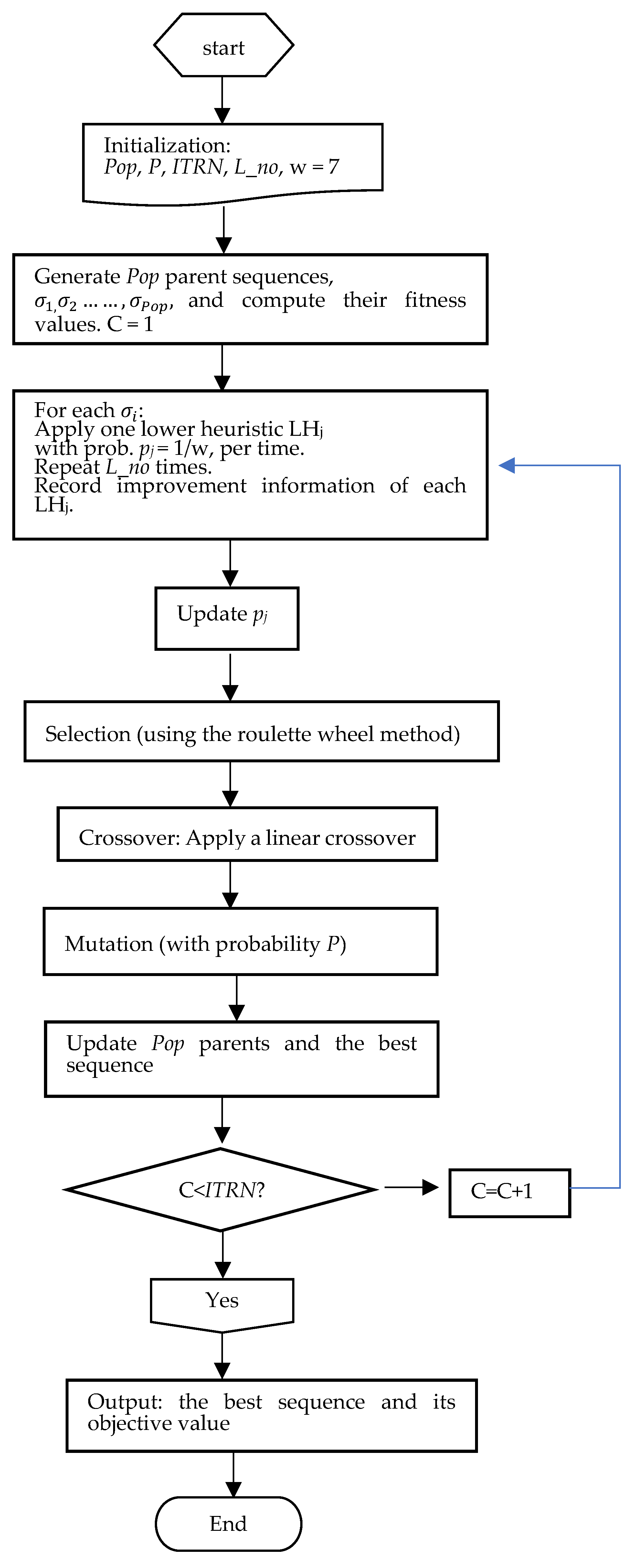
5. A Genetic and a Genetic Hyper-Heuristic

Most researchers have observed that in general, a heuristic seems relatively simple and easy to construct, whereas a metaheuristic is both complex and difficult to construct, as well as to use for intelligently implementing random search strategies [44,45]. The GA has been successfully utilized to obtain high-quality approximate solutions of many combinatorial problems. The GA is an effective computerized search tool for identifying the best and optimal solutions to complex problems based on genetic and neural selection mechanics such as mutation, crossover, and reproduction. These mutations have been used to successfully solve numerous NP-hard combinatorial problems. In the GA or GAHH (hyper-heuristic based on the GA framework), we applied a group of continuous real numbers to display the codes of orders by using a random-number encoding method. For example, given a chromosome (0.73, 0.62, 0.14, 0.23, 0.81) as a gene, we decoded it as a schedule (3, 4, 2, 1, 5) by using the ranking method. Specifically, in the reproduction stage, we selected the parents and recombined them by using a certain crossover operator to create offspring. In particular, in this study, we considered a linear order crossover (see Iyer and Saxena [46]). Moreover, the notations Pop, P, and IT_GA denote the number of parents, value of the mutation rate, and number of iterations (or generations), respectively, in executing the GA. The main structures of the proposed GA are summarized as follows:

Steps of genetic algorithm:

00:

InputPop, P, IT_GA.

01:

Generate a series of Pop initial parents (schedules) and find their fitness values.

02:

Do i = 1, IT_GA

03:

Choose two parents from Pop populations by using the roulette wheel method and employ a linear order crossover to reproduce a set of Pop offspring.

04:

For each offspring, generate a random number u (0 < u < 1) if u < P; then, create a new

05:

offspring by inserting a displacement mutation.

06:

Record the best one (schedule) and replace these Pop parents with their offspring.

07:

End do /* for the number of iterations (IT_GA) is fulfilled */

08:

Output the final best schedule and its fitness value.

In the following, a GA-based hyper-heuristic is applied to solve this problem by identifying problem-solving methods instead of directly finding solutions to the problem (refer to Cowling et al. [47] and Anagnostopoulos and Koulinas [48]). Hyper-heuristic processes have a high level of strategy and a low level of a group of heuristics that is used to determine a low-level heuristic to produce a new solution. Moreover, seven low-level heuristics are proposed on the basis of candidate variation operators such as the two-job swap heuristic, one step (or two steps) to the right heuristic, one step (or two steps) to the left heuristic, pulling-out and onward-moved reinsertion heuristic, and pulling-out and backward-moved reinsertion heuristic. Many studies have indicated that the two-job swapping method represents an effective improved scheme. To explore diverse search solutions, the randomly determined neighborhoods of a current job must be explored as well. They are recorded as LH₁, LH₂, …, and LH₇. The details of the proposed seven low-level heuristics are as follows:

LH₁:

Two-order swap heuristic: randomly select two orders (e.g., $O_2$ and $O_4$) in a schedule $\sigma$ and swap the selected two orders, resulting in a new schedule $\sigma \prime$. For example, $\sigma =\left(O_1, O_2, O_3, O_4, O_5\right)$, ${\sigma }^{\prime }=\left(O_1, O_4, O_3, O_2, O_5\right)$.

LH₂:

One step to the right heuristic: randomly select one order (e.g., $O_2$) in a schedule $\sigma$, extract order $O_2$ from its position, move it one position toward the right, and reinsert it to obtain a new schedule ${\sigma }^{\prime }$. For example, $\sigma =\left(O_1, O_2, O_3, O_4, O_5\right)$, ${\sigma }^{\prime }=\left(O_1, O_3, O_2, O_4, O_5\right)$.

LH₃:

Two steps to the right heuristic: randomly select one order (e.g., $O_3$) in a schedule $\sigma$, extract order $O_3$ from its position, move it two positions toward the right, and reinsert it, resulting in a new schedule ${\sigma }^{\prime }$. For example, $\sigma =\left(O_1, O_2, O_3, O_4, O_5\right)$, ${\sigma }^{\prime }=\left(O_1, O_2, O_4, O_5, O_3\right)$.

LH₄:

One step to the left heuristic: randomly select one order (e.g., $O_4$) in a schedule $\sigma$, extract job $O_4$ from its position, move it one position toward the left, and reinsert it, resulting in the new schedule ${\sigma }^{\prime }$. For example,$\sigma =\left(O_1, O_2, O_3, O_4, O_5\right)$, ${\sigma }^{\prime }=\left(O_1, O_2, O_4, O_3, O_5\right)$.

LH₅:

Two steps to the left heuristic: randomly select one order (e.g., $O_5$) in a schedule $\sigma$, extract order $O_5$ from its position, move it two positions toward the left, and reinsert it to obtain a new schedule ${\sigma }^{\prime }$. For example,$\sigma =\left(O_1, O_2, O_3, O_4, O_5\right)$, ${\sigma }^{\prime }=\left(O_1, O_2, O_5, O_3, O_4\right)$.

LH₆:

Pulling-out and onward-moved reinsertion heuristic: Randomly select two orders (e.g., $O_2$ and $O_5$) in a schedule $\sigma$, extract order $O_2$ (the leftward of the two selected orders) from its position, and onward reinsert it just after $O_5$ to obtain a new schedule ${\sigma }^{\prime }$. For example, $\sigma =\left(O_1, O_2, O_3, O_4, O_5\right)$, ${\sigma }^{\prime }=\left(O_1, O_3, O_4, O_5, O_2\right)$.

LH₇:

Pulling-out and backward-moved reinsertion heuristic: randomly select two orders (e.g., $O_2$ and $O_5$) in a schedule $\sigma$, extract order $O_5$ (the rightward of the two selected orders) from its position, and backward reinsert it just before $O_2$ to obtain a new schedule ${\sigma }^{\prime }$. For example,$\sigma =\left(O_1, O_2, O_3, O_4, O_5\right)$, ${\sigma }^{\prime }=\left(O_1, O_5, O_2, O_3, O_4\right)$.

Notably, as the value of n increases (for example, when n > 10,) in general, the operators LH₆ and LH₇ differ from the other five heuristics, especially when n = 100 or 200.

In what follows, the genetic algorthim hyper-heuristic is introduced based on the GA framework as well; it was labeled GAHH. In the execution of the GAHH, we randomly selected a low-level heuristic based on its selection probability and applied it once to each population over several iterations (named L_no). The current solution was replaced with a newly generated solution if the new solution was superior to the current solution; otherwise, it was accepted with a certain probability. Let $f_l=1/7$ be the initial probability of each LH_l; l = 1, 2, …, 7. Assume that ${\pi }_l$ is the recorded total frequency of obtaining a superior solution when cyclically executing LH_l. To ensure that all of the seven low-level heuristics in the pool were in the GAHH, we set ${\pi }_l=\max \left\{1,{\pi }_l\right\}$. The procedures of the GAHH were as follows:

Steps of genetic algorthim hyper-heuristic:

00:

InputPop, P, ITRN, L_no.

01:

Generate a series of Pop initial parents and find their fitness values.

02:

Do c = 1, ITRN

03:

set$f_l=1/7$, l = 1, 2, …, 7.

04:

Do i = 1, pop /* for each parent ${\sigma }_i$

05:

Dok = 1, L_no

06:

Select an $L{H}_l$ by using the roulette wheel method based on the value

07:

of $f_l$ to improve ${\sigma }_i$ for generating another new schedule ${\sigma }_t$.

08:

Replace ${\pi }_l={\pi }_l+1$ with LH_j if RC(${\mathsf{\sigma }}_t$) < RC(${\sigma }_i$).

09:

Retain each superior current parent ${\sigma }_i$

10:

End do /* for the low-level heuristics */

11:

End do /* i = 1, 2, …, Pop */

12:

Update the probabilities $\{f_l$, l = 1, 2, …, 7} of ${\mathrm{LH}}_1$, ${\mathrm{LH}}_2$, …, and ${\mathrm{LH}}_7$ according

13:

their past records as {$f_l={\pi }_l/\sum _{j=1}^7{\pi }_j, l=1,\dots$,7}

14:

Select two parents from Pop populations by using the roulette wheel method and

15:

employ a linear order crossover to reproduce a set of Pop offspring.

16:

For each offspring, generate a random number u (0 < u < 1) if u < P; then, create a

17:

new offspring by inserting a displacement mutation.

18:

Retain the best offspring, and replace the parents of this Pop with their offspring.

19:

End do /*when the iterative number of high-level cycles (ITRN) is */

20:

Output the final best sequence and its fitness value.

The flowchart of the GAHH is depicted in Figure 1.

To find an exact solution for small-sized orders, the best of the schedules found using the three proposed heuristics, a GA, and the GAHH was used as the upper bound in a depth-first B&B method. To help cut the branching trees, the proposed properties and the lower bound were used in the method. The orders were first scheduled in a forward manner, and we selected a systematic search and branch down each tree [25,28,34,36].

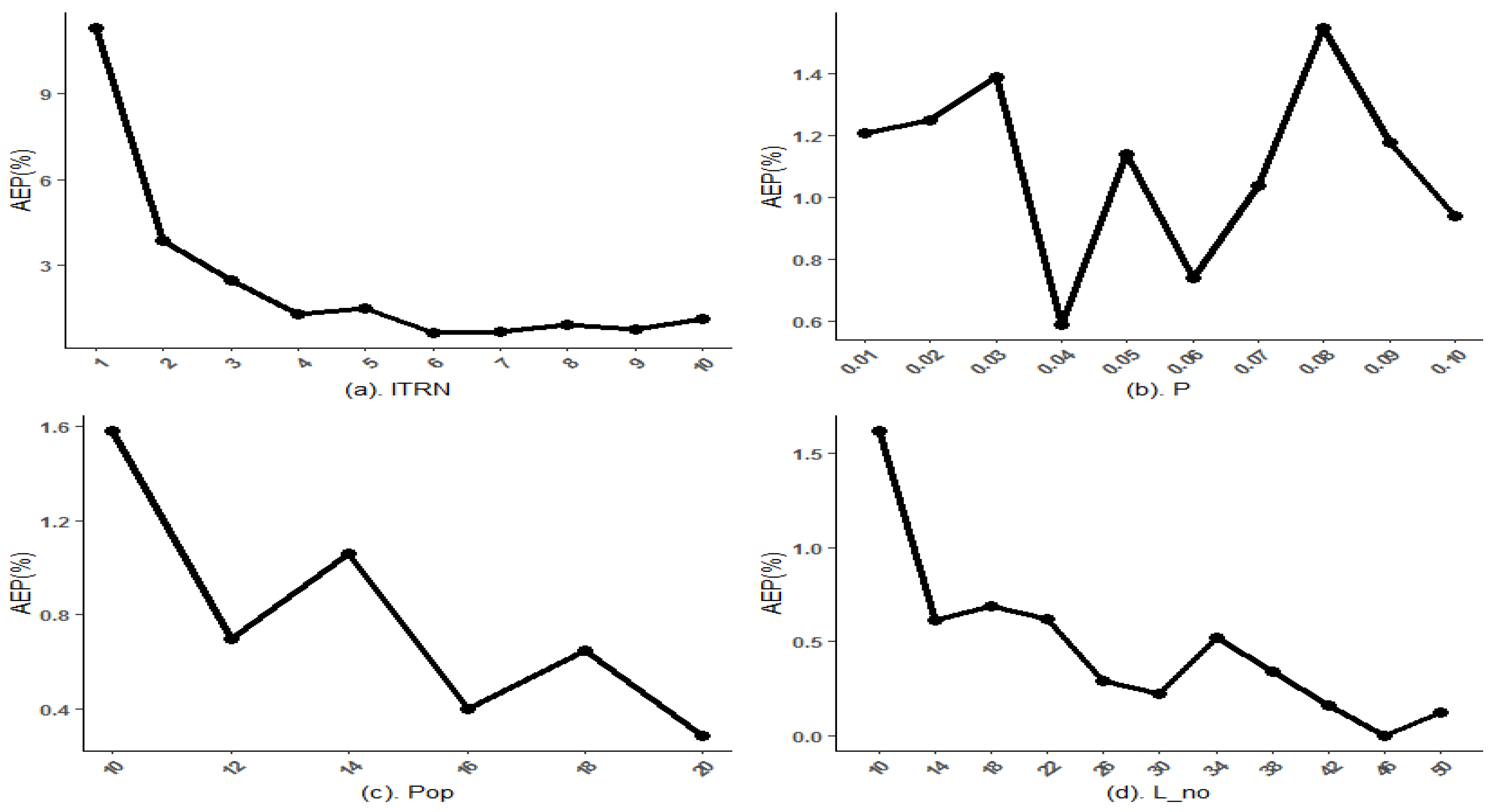
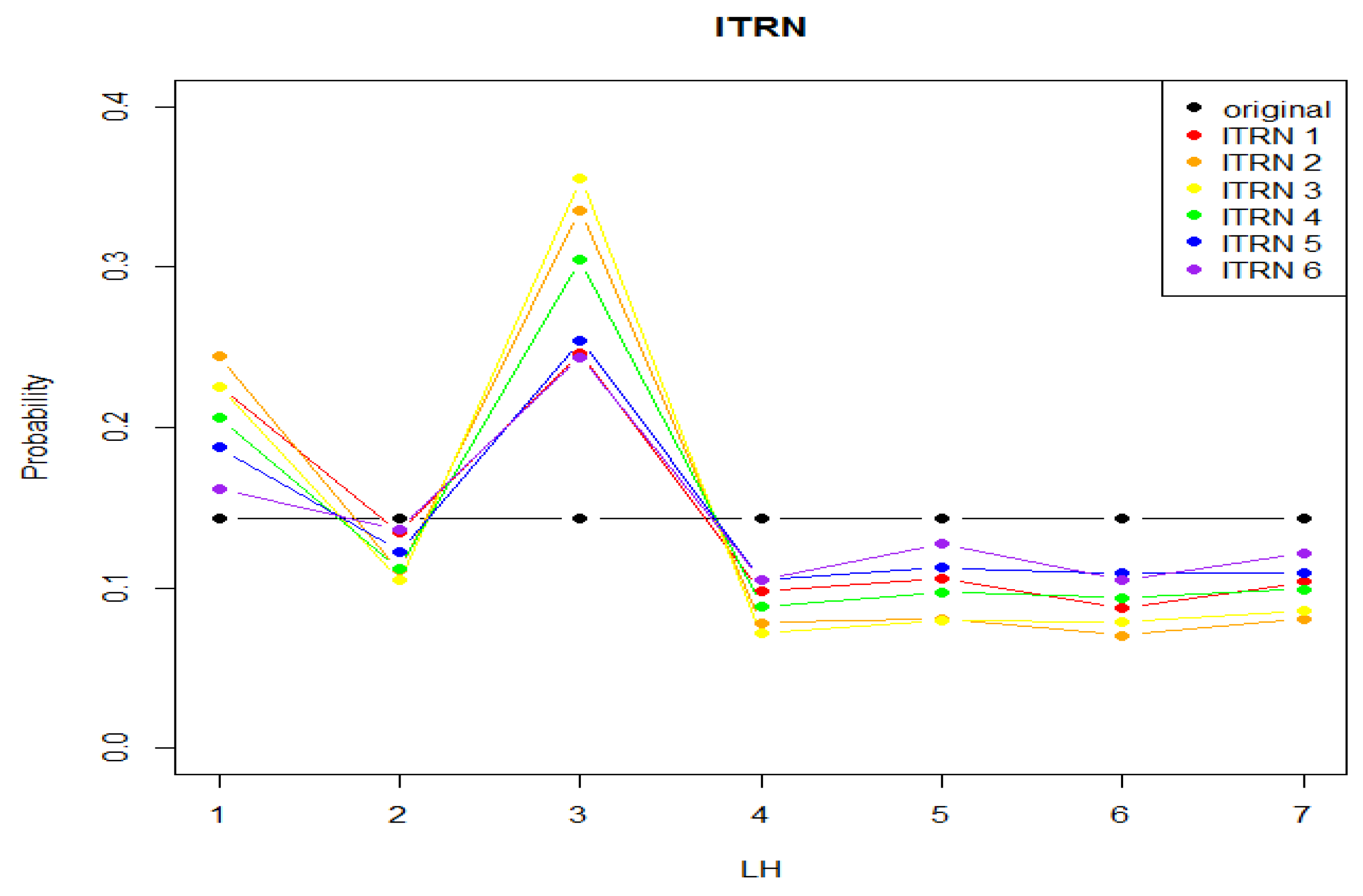
6. Tuning Genetic Algorithm Hyper-Heuristic Parameters

With reference to the scheme of Montgomery [49], in this section, we present an approach that used one factor at a time to tune the relevant GAHH parameters. The GAHH proposed in Section 5 had four parameters; namely, population size (Pop), number of low-level heuristics applied (L_no), mutation probability (P), and number of high-level cycles (ITRN). To reduce the computation time or obtain superior solutions, the values of these parameters must be tuned before conducting a simulation study. To obtain suitable parameter settings, we computed the average error percentage (AEP) as AEP = 100$\sum _{i=1}^n(\frac{H_i-B_i^{*}}{B_i^{*}})$[%], where H_i is the objective solution searched using the GAHH, and $B_i^{*}$ is the optimal objective value obtained using the B&B method for each instance i. With reference to the designs of Leung et al. [10,11,12,13,14,16], Lee [20], Lin et al. [28], and Yang and Yu [33], the weights $w_i$ were generated from the uniform distribution U (1, 100). The component processing time $t_{iv}^{\left(1\right)}$ and ready time $r_i^{\left(1\right)}$ of an order were generated from the uniform distributions U (1, 100) and U (1, $100\times \mathrm{n}\times \mathsf{\lambda }$); the due dates of an order were generated from the uniform distribution U (TPTbar(1) (1 − τ − ρ/2), TPTbar(1) (1 − τ + ρ/2)) in Scenario 1. In Scenario 2, the component processing time $t_{iv}^{\left(2\right)}$ and ready time $r_i^{\left(2\right)}$ of an order were generated from the uniform distributions U (1, 200) and U (1, $200\times \mathrm{n}\times \mathsf{\lambda }$), and the due dates of an order were generated from the uniform distribution U (TPTbar(2) (1 − τ − ρ/2), TPTbar(2) (1 – τ + ρ/2)), where $TPTbar\left(s\right)=\sum _{v=1}^m\sum _{i=1}^n{t}_{iv}^{\left(s\right)}/m$; τ and ρ describe the tardiness factor and range of due dates, respectively; and $0<\mathsf{\lambda }<1$ is a controllable parameter. For simplification, we set n = 10, m = 3, τ = 0.5, ρ = 0.5, and $\mathsf{\lambda }=0.3$ and generated 100 problem instances for testing.

With Pop = 10, P = 0.05, and L_no = 20, a simulation was conducted and designed as ITRN was varied from 1 to 10 in incremental steps of 1. It can be seen in Figure 2a that the lowest point of the AEP was located at ITRN = 6. With Pop = 10, ITRN = 6, and L_no = 20, a simulation was conducted and designed as P was varied from 0.01 to 0.1 in incremental steps of 0.1. It can be seen in Figure 2b that the AEP was approximately zero (below 0.59%) when P was 0.04, which indicated an effective reduction in the AEP. With ITRN = 6, P = 0.04, and L_no = 20, a simulation was conducted and designed as Pop was varied from 10 to 20 in incremental steps of 2. It can be seen in Figure 2c that the AEP was the minimum (~0.29%) when Pop = 20, which indicated an effective reduction in the AEP with an increase in Pop. With ITRN = 6, P = 0.04, and Pop = 20, a simulation was conducted and designed as L_no was varied from 10 to 50 in incremental steps of 4. It can be seen in Figure 2d that the AEP was the lowest (~0.03%) when L_no equaled 46.

Finally, the optimal setting values of the parameter (Pop, P, ITRN, L_no) were set to (20, 0.04, 6, 46) for small-sized orders. However, for large-sized orders, where n = 100 and 200, a greater number of lower-level heuristics (L_no) was required to obtain superior solutions; following the same approach as above, we eventually set L_no to 560 and 1000 for n = 100 and n = 200, respectively, for use in subsequent simulation studies.

Notably, three stopping conditions are commonly used in metaheuristics; namely, the number of generations, the difference between the current best solution and the previous best solution, and the limitation of CPU time. To fairly compare the proposed GAHH and GA, the same values for the population size, the same crossover scheme, and the same mutation rates were used in both approaches. We only revised the number of generations (IT_GA) in case of the GA to approximate to the number of repeated cycles (ITRN) multiplied by the times of the low-level heuristics per cycle (L_no) in the GAHH, that is, IT_GA = ITRN × L_no. After our preliminary tests, the parameters (Pop, P, IT_GA) in the GA method were set to (20, 0.04, 276) for small-sized orders (n = 9, 11), (20, 0.04, 3360) for n = 100, and (20, 0.04, 6000) for n = 200, respectively. Due to the integration of high-level strategic heuristics with a group of low-level heuristics, a small GAHH population was adequate.

7. Simulation Study

In this section, the performances of the B&B method, three heuristics, the GA, and the GAHH were evaluated through simulation studies. All of the algorithms were coded in FORTRAN and executed on a personal computer equipped with an Intel Core i7 CPU (2.66 GHz) and 4 GB of RAM and running the Windows XP operating system. With reference to the design of Leung et al. [10,12,13,14], Lee [20], and Lin et al. [28], we generated the component processing times $t_{iv}^{\left(1\right)}$ from U (1, 100) for the order instances in Scenario 1. The $t_{iv}^{\left(2\right)}$ values of an order i on m machines were independently obtained from U (1, 200) for m = 2, 3, and 4 (small-sized orders) and m = 5, 10, and 20 (large-sized orders). The weight w_i of each order was randomly generated from another U (1, 100) independently. In addition, we generated the due dates of the orders from another U (TPTbar(s) (1 − τ − ρ/2), TPTbar(s) (1 – τ + ρ/2)), where $TPTbar\left(s\right)=\sum _{v=1}^m\sum _{i=1}^n{t}_{iv}^{\left(s\right)}/m$, τ denotes the tardiness factor, and ρ denotes range of due dates. The combinations of (τ, ρ) included (0.25, 0.25), (0.25, 0.5), (0.5, 0.75), (0.5, 0.5), (0.5, 0.25), and (0.25, 0.75). With reference to the design of Reeves [50], we generated the ready times from U (1, 100nλ) for Scenario 1 and U (1, 200nλ) for Scenario 2, respectively, where λ is the control variable. The value of λ was set to 0.1, 0.3, and 0.5. Herein, the two parts of the simulation study were designed to address small- and large-sized orders.

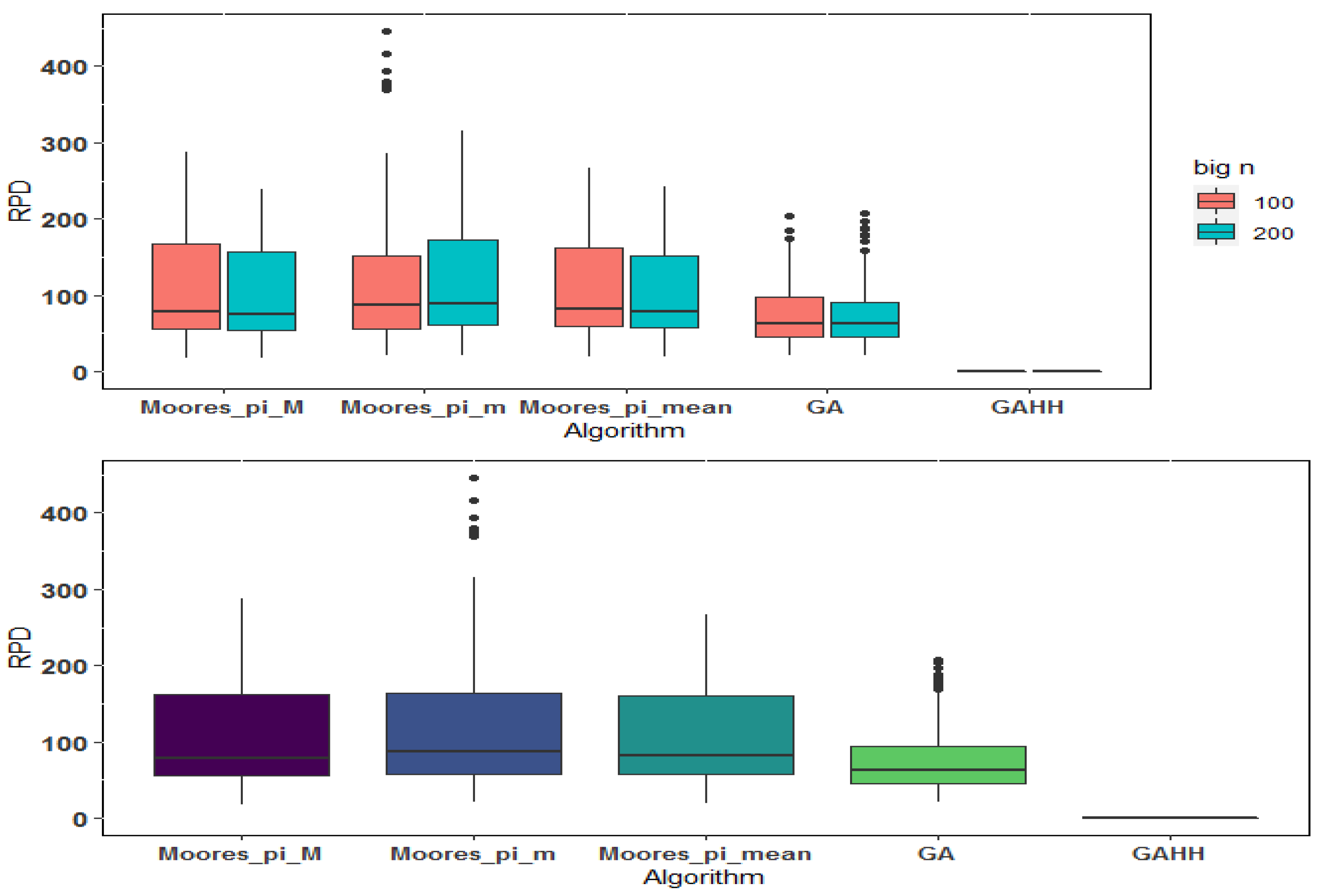
7.1. Results Obtained for Small-Sized Orders

For the small-sized orders, the number of orders n was set as 9 and 11 and the number of machines m as 2, 3, and 4. A total of 100 problem instances were examined for each combination of (n, m, λ, τ, ρ). Thus, in total, 10,800 (=100·2·3·3·2·3) instances were tested in this experiment. The B&B method was set to stop and run the next instance when the number of trimmed nodes exceeded 10⁸.

The average and maximum number of nodes and the average and maximum execution times (in seconds) were recorded to determine the performance of the B&B method. To assess the performance of the three modified Moore’s heuristics, GA, and GAHH, the AEP and maximum error percentage were recorded. The performance of the B&B method is summarized in

Table 1. Number of B&B nodes and CPU time for small values of n.

		Node		CPU_Time
n	m	Mean	Max	Mean	Max
9	2	102,150	35,6594	0.56	1.25
	3	108,842	35,9043	0.68	1.48
	4	116,378	386,330	0.82	1.79
11	2	606,5047	25,997,813	57.42	193.89
	3	6,701,240	27,681,786	74.84	235.82
	4	6,952,756	27,613,651	90.24	272.42
Mean		3,341,069	1,373,2536	37.43	117.78
n	$\mathsf{\lambda }$	Mean	Max	Mean	Max
9	0.1	63,883	15,8272	0.52	1.11
	0.3	84,005	374,265	0.61	1.56
	0.5	179,482	569,430	0.93	1.86
11	0.1	316,9517	9,901,037	47.60	131.62
	0.3	4,378,853	21,526,663	61.14	236.57
	0.5	12,170,673	49,865,551	113.76	333.93
Mean		3,341,069	13,732,536	37.43	117.78
n	$\tau$	Mean	Max	Mean	Max
9	0.25	73,284	287,313	0.55	1.40
	0.50	144,963	447,331	0.82	1.62
11	0.25	3,734,194	17,472,356	53.12	200.44
	0.50	9,411,835	36,723,144	95.21	267.64
Mean		3,341,069	13,732,536	37.43	117.78
n	$\rho$	Mean	Max	Mean	Max
9	0.25	120,476	374,104	0.71	1.49
	0.50	105,302	379,570	0.67	1.51
	0.75	101,593	348,294	0.68	1.53
11	0.25	7,668,642	29,579,795	80.48	255.49
	0.50	6,353,625	26,905,933	71.67	225.25
	0.75	5,696,776	24,807,523	70.35	221.39
Mean		3,341,069	13,732,536	37.43	117.78

. The performances of the proposed heuristics and algorithms are summarized in

Table 2. AEPs of the proposed heuristics and algorithms for small n.

		Moores_pi_M		Moores_pi_m		Moores_pi_Mean		GA		GAHH
n	m	Mean	Max	Mean	Max	Mean	Max	Mean	Max	Mean	Max
9	2	63.19	684.27	63.39	851.01	65.54	650.55	18.47	278.18	0.77	26.61
	3	47.03	335.87	45.22	355.35	47.88	284.18	15.21	130.37	0.35	14.42
	4	45.80	319.15	43.15	237.90	45.31	307.29	13.79	92.95	0.32	14.15
11	2	81.46	478.10	78.19	448.14	83.70	448.73	26.99	226.09	2.45	69.87
	3	68.64	467.13	64.53	460.21	70.29	473.65	22.55	121.51	1.89	33.21
	4	66.44	432.34	62.17	326.86	66.07	340.21	21.62	125.73	1.55	27.67
Mean		62.09	452.81	59.44	446.58	63.13	417.44	19.77	162.47	1.22	30.99
$n$	$\lambda$	Mean	Max	Mean	Max	Mean	Max	Mean	Max	Mean	Max
9	0.1	107.49	1009.37	103.09	1121.00	108.48	927.90	27.76	348.97	1.10	34.63
	0.3	38.61	220.82	37.83	248.44	39.25	234.59	14.14	106.10	0.26	16.50
	0.5	9.92	75.27	10.84	74.82	11.01	79.53	5.57	46.44	0.07	4.04
11	0.1	148.71	990.73	134.73	822.99	148.81	891.54	41.34	303.50	4.46	98.83
	0.3	53.71	301.37	54.70	323.03	55.24	282.37	21.32	116.75	1.12	18.92
	0.5	14.12	85.47	15.46	89.19	16.01	88.67	8.50	53.08	0.30	13.01
Mean		62.09	447.17	59.44	446.58	63.13	417.43	19.77	162.47	1.22	30.99
n	τ	Mean	Max	Mean	Max	Mean	Max	Mean	Max	Mean	Max
9	0.25	84.43	796.07	82.39	871.91	85.42	727.47	24.21	271.87	0.75	26.91
	0.50	19.58	100.94	18.78	90.93	20.40	100.54	7.44	62.47	0.20	9.87
11	0.25	116.61	813.22	110.02	722.44	117.08	735.28	35.40	260.65	3.16	70.70
	0.50	27.75	105.17	26.57	101.04	29.63	106.44	12.04	54.90	0.76	16.47
Mean		62.09	453.85	59.44	446.58	63.13	417.43	19.77	162.47	1.22	30.99
$n$	$\rho$	Mean	Max	Mean	Max	Mean	Max	Mean	Max	Mean	Max
9	0.25	38.27	233.89	37.68	247.73	38.07	212.74	11.73	75.19	0.47	19.79
	0.50	53.90	296.54	51.15	289.09	54.89	294.14	16.97	122.25	0.51	18.54
	0.75	63.85	816.19	62.93	907.44	65.77	735.13	18.77	304.06	0.45	16.85
11	0.25	51.33	272.43	52.18	292.91	52.07	280.87	17.25	97.82	1.01	21.54
	0.50	75.80	463.10	72.77	441.39	77.43	416.31	25.34	169.34	1.81	31.39
	0.75	89.40	642.04	79.93	500.92	90.56	565.40	28.57	206.17	3.07	77.82
Mean		62.09	454.03	59.44	446.58	63.13	417.43	19.77	162.47	1.22	30.99

.

The effects of the parameters on the execution of the B&B method are summarized in Table 1. The averages of the mean nodes and CPU time increased dramatically as n was increased from 9 to 11 regardless of the parameter. This phenomenon illustrated one characteristic of an NP-hard problem. The number of machines and ρ had little effect on the performance of the B&B method. In terms of the effects of the parameters m, λ, and τ on the mean number of nodes in the B&B method, the means of both the number of nodes and CPU time tended to increase for both n = 9 and n = 11 as the value of one of these parameters was increased and the other parameters were fixed. The number of nodes and CPU time decreased as the value of ρ increased for both values of n. This result implied that in the instances with a smaller value, the optimal solution was easily obtained using the B&B method.

In terms of the effects of the aforementioned parameters on the performance of the three Moore’s-type heuristics, the mean AEPs of the three heuristics, GA, and GAHH tended to decrease as the value of m, λ, or τ increased (Table 2). In contrast, the mean AEP of the three heuristics and both GAs increased as the value of ρ increased. Moreover, the results in Table 2 confirmed that on average, the GAHH outperformed the other algorithms.

To compare the solution quality among the Moore_pi_M, Moore_pi_m, Moore_pi_mean, GA, and GAHH (with mean AEPs of 62.09, 59.44, 63.13, 19.77, and 1.22, respectively), the AEPs obtained under variations in different factors including the algorithm; number of jobs; number of machines; and the parameters λ, τ, and ρ were fitted to a linear model. The analysis of variance results for the AEP revealed significant differences in the performance of all factors when the significance level was 0.05, but the normality of the error term was significantly invalid as indicated by a Shapiro–Wilk test (with the statistic = 0.8535 and p < 0.0001). The boxplots in Figure 3 display the AEP distributions of all the proposed heuristics and algorithms. Accordingly, a nonparametric statistical method was used to perform multiple comparisons between these methods. Then, a Freidman test (with p < 0.0001) showed that the AEP samples were not followed the same distribution under a significance level of 0.05 according to the basis of AEP ranks on the 108 (n·m·λ·τ·ρ = 2·3·3·2·3) blocks of test problem instances.

Furthermore, to find the pairwise differences among the three heuristics, GA, and GAHH, we conducted a Wilcoxon–Nemenyi–McDonald–Thompson (WNMT) test (see chapter 7 in Hollander et al. [51]).

Table 3. Nonparametric multiple comparisons of AEP and relative percentage deviation.

	Small Job Size n		Large Job Size n
Pairwise Comparison between Algorithm	|Pairwise Rank-Sum Difference|	Difference > 64.4 *	|Pairwise Rank-Sum Difference|	Difference > 64.4 *
Moores_pi_M vs. Moores_pi_m	|401.0–414.0|	NO	|359.0–496.0|	YES
Moores_pi_M vs. Moores_pi_mean	|401.0–472.0|	YES	|359.0–402.0|	NO
Moores_pi_M vs. GA	|401.0–223.0|	YES	|359.0–255.0|	YES
Moores_pi_M vs. GAHH	|401.0–110.0|	YES	|359.0–108.0|	YES
Moores_pi_m vs. Moores_pi_mean	|414.0–472.0|	NO	|496.0–402.0|	YES
Moores_pi_m vs. GA	|414.0–223.0|	YES	|496.0–255.0|	YES
Moores_pi_m vs. GAHH	|414.0–110.0|	YES	|496.0–108.0|	YES
Moores_pi_mean vs. GA	|472.0–223.0|	YES	|402.0–255.0|	YES
Moores_pi_mean vs. GAHH	|472.0–110.0|	YES	|402.0–108.0|	YES
GA vs. GAHH	|223.0–110.0|	YES	|255.0–108.0|	YES

* Approximated using a formula reported in Hollander et al. [51], page 316.

lists the sum of ranks of AEPs for the three heuristics, GA, and GAHH. The behaviors of all of the proposed algorithms could be grouped into four groups under a significance level of 0.05. As can be inferred from columns 2 and 3 of Table 3, the performance of the GAHH was the best (rank-sum = 110.0) followed by GA (rank-sum = 223), whereas Moores_pi_m and Moores_pi_mean (rank-sums = 414.0 and 472.0, respectively) exhibited the poorest performances.

As for the usage of the seven low-level heuristics, the variations in the probabilities of them being called in the GAHH are displayed in Figure 4. HL₃ was called most frequently and was typically followed by HL₁. However, HL₄, HL₅, HL₆, and HL₇ were rarely called.

7.2. Results for Large-Sized Orders

For a large number of jobs, we set the order size n to 100 and 200 and the number of machines m to 5, 10, and 20. One hundred problem instances were randomly examined for each parameter combination. Consequently, a total of 10,800 (=100·2·3·3·2·3) problem instances were examined in this simulation. To evaluate the performance of the three heuristics, GA, and GAHH, we reported the mean and maximum relative percentage deviation (RPD). RPD is defined as follows: RPD = 100$\sum _{i=1}^n(\frac{H_i-H^{*}}{H^{*}})$[%], where $H_i$ is the value of the objective function searched for using the three heuristics, GA, and GAHH; and H* is the minimum among these five methods for each instance. The RPDs obtained with variations in n, m, λ, τ, and ρ are summarized in

Table 4. RPDs obtained using proposed heuristics and algorithms for large n.

		Moores_pi_M		Moores_pi_m		Moores_pi_Mean		GA		GAHH
n	m	Mean	Max	Mean	Max	Mean	Max	Mean	Max	Mean	Max
100	5	117.98	190.76	134.45	225.48	115.52	194.47	79.90	143.19	0.00	0.00
	10	111.11	175.04	127.34	213.33	108.83	174.50	74.67	126.33	0.00	0.00
	15	107.61	196.72	123.20	207.02	105.71	201.19	72.78	130.91	0.00	0.00
200	5	105.19	154.86	127.30	180.75	105.31	156.38	81.17	123.84	0.00	0.00
	10	100.35	146.16	120.94	172.32	99.54	151.17	77.28	114.04	0.00	0.00
	15	97.85	144.41	118.07	166.99	97.77	139.84	74.94	109.50	0.00	0.00
Mean		106.68	167.99	125.22	194.32	105.45	169.59	76.79	124.64	0.00	0.00
n	λ	Mean	Max	Mean	Max	Mean	Max	Mean	Max	Mean	Max
100	0.1	184.26	323.65	235.51	406.75	174.74	320.61	114.44	212.68	0.00	0.00
	0.3	109.43	168.40	103.81	162.00	109.91	175.22	71.13	118.47	0.00	0.00
	0.5	43.02	70.46	45.67	77.09	45.42	74.33	41.78	69.28	0.00	0.00
200	0.1	161.27	245.04	210.16	302.04	158.99	243.33	124.74	189.48	0.00	0.00
	0.3	101.68	139.58	110.93	150.51	101.66	141.29	68.45	98.37	0.00	0.00
	0.5	40.45	60.81	45.22	67.52	41.97	62.76	40.21	59.54	0.00	0.00
Mean		106.68	167.99	125.22	194.32	105.45	169.59	76.79	124.64	0.00	0.00
n	τ	Mean	Max	Mean	Max	Mean	Max	Mean	Max	Mean	Max
100	0.25	158.29	274.79	190.88	332.02	155.80	284.64	106.99	195.69	0.00	0.00
	0.50	66.18	100.22	65.78	98.53	64.24	95.47	44.58	71.27	0.00	0.00
200	0.25	139.15	209.37	170.33	245.76	139.91	212.30	110.48	167.20	0.00	0.00
	0.50	63.12	87.58	73.87	100.95	61.83	85.96	45.12	64.39	0.00	0.00
Mean		106.68	167.99	125.22	194.32	105.45	169.59	76.79	124.64	0.00	0.00
n	ρ	Mean	Max	Mean	Max	Mean	Max	Mean	Max	Mean	Max
100	0.25	93.79	156.60	108.21	173.59	94.62	160.03	70.15	119.17	0.00	0.00
	0.50	117.33	211.28	134.50	232.41	115.43	217.54	79.01	145.33	0.00	0.00
	0.75	125.60	194.63	142.28	239.83	120.02	192.59	78.19	135.93	0.00	0.00
200	0.25	86.77	128.64	106.01	146.45	89.63	129.30	73.60	107.26	0.00	0.00
	0.50	105.66	155.60	126.86	181.39	105.13	156.28	81.10	122.02	0.00	0.00
	0.75	110.97	161.18	133.44	192.22	107.86	161.80	78.70	118.10	0.00	0.00
Mean		106.68	167.99	125.22	194.32	105.45	169.59	76.79	124.64	0.00	0.00

.

As summarized in Table 4, the average RPDs of the three modified Moore’s-type heuristics and the GA strictly decreased as the number of machines and values of the parameters λ and τ increased for n = 100 and 200. In contrast, the average RPDs of the three Moore’s-type heuristics decreased as the value of ρ increased. Moreover, with an average RPD of close to 0 for both values of n, the GAHH outperformed the other methods.

The boxplots of the RPDs of the five algorithms are depicted in Figure 5. The GAHH outperformed the other four algorithms when n was large. Overall, the average RPDs of the Moores_pi_M, Moores_pi_m, Moores_pi_mean, GA, and GAHH approaches were 106.68, 125.22, 105.45, 76.79, and 0.00, respectively. The experimental results further corroborated the superiority of the GAHH approach.

In view of the significant differences in the average RPDs of the three heuristics, GA, and GAHH, we performed an analysis to confirm the differences and make direct pairwise comparisons statistically. Another linear model that was run in the SAS 9.4 environment was fitted to the RPDs obtained under variations in different factors including the algorithm; number of jobs and machines; and parameters λ, τ, and ρ. Subsequently, the normality of the error term was tested for significance by running the Shapiro–Wilk test (statistic = 0.9114 and p < 0.0001) under a significance level of 0.05. A nonparametric statistical method—the WNMT test—was used to make multiple comparisons of the performance of the five algorithms. Table 3 lists the sum of ranks of RPDs of the three proposed heuristics, GA, and GAHH. The performance levels of all proposed algorithms could be grouped into four groups at the 0.05 significance level. As can be inferred from columns 4 and 5 of Table 3, the GAHH (rank-sum = 108.0) yielded the best performance followed by the GA (rank-sum = 255), whereas Moores_pi_m (rank-sum = 496) yielded the poorest performance.

The CPU times of all of the proposed algorithms were extremely short in the small-order-size case; thus, they were omitted here.

Table 5. CPU times obtained with proposed heuristics and algorithms for large n.

		Moore_pi_M		Moore_pi_m		Moore_pi_Mean		GA		GAHH
$\mathit{n}$	m	Mean	Max	Mean	Max	Mean	Max	Mean	Max	Mean	Max
100	5	0.04	0.05	0.04	0.05	0.04	0.05	0.01	0.02	0.51	0.58
	10	0.07	0.09	0.07	0.09	0.07	0.09	0.01	0.03	0.91	1.01
	15	0.10	0.13	0.10	0.13	0.10	0.13	0.01	0.04	1.33	1.52
200	5	0.28	0.35	0.28	0.33	0.29	0.35	0.01	0.03	1.78	1.98
	10	0.50	0.67	0.49	0.57	0.49	0.56	0.02	0.05	3.11	3.47
	15	0.90	1.13	0.83	1.05	0.83	1.07	0.03	0.08	5.21	6.46
mean		0.32	0.40	0.30	0.37	0.30	0.38	0.02	0.04	2.14	2.50
$n$	$\lambda$	Mean	Max	Mean	Max	Mean	Max	Mean	Max	Mean	Max
100	0.1	0.07	0.09	0.07	0.09	0.07	0.09	0.01	0.03	0.90	1.01
	0.3	0.07	0.09	0.07	0.09	0.07	0.09	0.01	0.03	0.89	1.01
	0.5	0.07	0.09	0.07	0.09	0.07	0.09	0.01	0.02	0.91	1.02
200	0.1	0.51	0.62	0.49	0.59	0.51	0.61	0.03	0.06	3.22	3.65
	0.3	0.54	0.69	0.52	0.64	0.53	0.66	0.03	0.07	3.42	4.26
	0.5	0.61	0.78	0.56	0.68	0.55	0.67	0.01	0.03	3.28	3.80
mean		0.31	0.39	0.30	0.36	0.30	0.37	0.02	0.04	2.10	2.46
n	τ	Mean	Max	Mean	Max	Mean	Max	Mean	Max	Mean	Max
100	0.25	0.07	0.09	0.07	0.09	0.07	0.09	0.01	0.03	0.93	1.05
	0.50	0.07	0.09	0.07	0.09	0.07	0.09	0.01	0.03	0.91	1.02
200	0.25	0.55	0.69	0.53	0.64	0.53	0.64	0.03	0.06	3.39	4.00
	0.50	0.58	0.75	0.54	0.66	0.54	0.68	0.02	0.05	3.35	3.94
mean		0.32	0.41	0.30	0.37	0.30	0.38	0.02	0.04	2.15	2.50
$n$	$\rho$	Mean	Max	Mean	Max	Mean	Max	Mean	Max	Mean	Max
100	0.25	0.07	0.09	0.07	0.09	0.07	0.09	0.01	0.03	0.92	1.05
	0.50	0.07	0.10	0.07	0.09	0.07	0.09	0.01	0.03	0.91	1.02
	0.75	0.07	0.09	0.07	0.09	0.07	0.09	0.01	0.03	0.93	1.05
200	0.25	0.56	0.70	0.52	0.63	0.53	0.65	0.02	0.05	3.34	3.97
	0.50	0.55	0.70	0.53	0.63	0.53	0.66	0.02	0.06	3.38	3.99
	0.75	0.58	0.75	0.54	0.68	0.55	0.67	0.03	0.06	3.38	3.96
mean		0.32	0.41	0.30	0.37	0.30	0.38	0.02	0.04	2.14	2.51

lists the CPU times of all of the proposed heuristics and metaheuristics in the large-order-size case. As summarized and illustrated in Table 5 and Figure 6, respectively, on average, the AEPs of the Moore_pi_M, Moore_pi_m, Moore_pi_mean, GA, and GAHH approaches were 0.32, 0.30, 0.30, 0.02, and 2.14, respectively, in the large-order-size case regardless of the parameter values, except for the number of orders (n). Furthermore, in terms of the differences between the GA and GAHH, under the same design with the same population, the same mutation, and It_GA = ITRN × L_no, the computation time of the GAHH was 2 s longer than that of the GA because the GAHH required considerable CPU time to select low-level heuristics. In the worst case, GAHH required 8.02 s to solve an instance. However, the mean of the maximum solving times of the GAHH approach was 2.51 s. This result confirmed that the GAHH approach maintained a small population and limited the number of generations required for obtaining a high-quality solution.

On the basis on the test results, we concluded that the GAHH, on average, outperformed the other heuristics and the GA in the simulation tests regardless of the order size.

8. Conclusions and Future Work

Customer order scheduling models have emerged as a major challenge in manufacturing environments and practical applications (Framinan et al. [4]). Diverging from the common assumption that component processing times, ready times, and due dates are fixed, this study investigated cases involving scenario-dependent component processing times, ready times, and due dates; the objective was to find an appropriate and robust sequence of orders to minimize the maximum of the sum of weighted tardy orders across the considered scenarios. To solve this problem, first, dominance properties and a lower bound were derived and a B&B method was applied to search for the optimal solutions for small-sized orders. Second, three variants (heuristics) of Moore’s algorithm and the GAHH were developed along with a conventional GA to obtain approximate solutions for large-sized orders. Simulations were performed to evaluate the capability of the B&B method and the effects of parameter values on its performance. The experimental results obtained by considering the dominance properties and the derived lower bound indicated that the B&B method could solve problem instances with n values up to 11 within a reasonable CPU time (Table 1). The experimental tests further demonstrated that the GA and GAHH performed satisfactorily in term of efficacy and efficiency for problem instances involving both small- and large-sized orders. In the case of the GAHH with a scheme for randomly selecting from among seven operators, we only required a small population and a small number of iterative cycles (ITRN) to obtain a high-quality solution compared with the GA without a neighborhood heuristic. Overall, on the basis of the simulation results, we can recommend using the GAHH approach to solve the problem considered herein due to its superior performance and speed in attaining high-quality solutions in terms of the AEP and RPD. In the future, researchers can investigate the COSP with more than three scenario-dependent processing times as well as order rejection based on different criteria; for example, the total completion time, the makespan, or even a multiobjective case. Another direction for future study could involve using the GAHH with seven versions to evaluate the impact of having no operator, one operator, and multiple operators.

References

1. Ahmadi, R.; Bagchi, U.; Roemer, T.A. Coordinated scheduling of customer orders for quick response. Nav. Res. Logist. 2005, 52, 493–512. [Google Scholar] [CrossRef]
2. Guo, Q.; Tang, L. Modelling and discrete differential evolution algorithm for order rescheduling problem in steel industry. Comput. Ind. Eng. 2019, 130, 586–595. [Google Scholar] [CrossRef]
3. Zhang, Y.; Dan, Y.; Dan, B.; Gao, H. The order scheduling problem of product-service system with time windows. Comput. Ind. Eng. 2019, 133, 253–266. [Google Scholar] [CrossRef]
4. Framinan, J.M.; Perez-Gonzalez, P.; Fernandez-Viagas, V. Deterministic assembly scheduling problems: A review and classification of concurrent-type scheduling models and solution procedures. Eur. J. Oper. Res. 2019, 273, 401–417. [Google Scholar] [CrossRef] [Green Version]
5. Framinan, J.; Perez-Gonzalez, P. New approximate algorithms for the customer order scheduling problem with total completion time objective. Comput. Oper. Res. 2017, 78, 181–192. [Google Scholar] [CrossRef]
6. Sung, C.S.; Yoon, S.H. Minimizing total weighted completion time at a pre- assembly stage composed of two feeding machines. Int. J. Prod. Econ. 1998, 54, 247–255. [Google Scholar] [CrossRef]
7. Yoon, S.H.; Sung, C.S. Fixed pre-assembly scheduling on multiple fabrication machines. Int. J. Prod. Econ. 2005, 96, 109–118. [Google Scholar] [CrossRef]
8. Wang, G.; Cheng, T.C.E. Customer order scheduling to minimize total weighted completion time. Omega 2007, 35, 623–626. [Google Scholar] [CrossRef] [Green Version]
9. Leung, J.Y.T.; Li, H.; Pinedo, M.; Sriskandarajah, C. Open shops with jobs overlap-revisited. Eur. J. Oper. Res. 2005, 163, 569–571. [Google Scholar] [CrossRef]
10. Leung, J.Y.T.; Li, H.; Pinedo, M. Approximation algorithms for minimizing total weighted completion time of orders on identical machines in parallel. Nav. Res. Logist. 2006, 53, 243–260. [Google Scholar] [CrossRef]
11. Leung, J.Y.T.; Li, H.; Pinedo, M. Scheduling orders for multiple product types to minimize total weighted completion time. Discret. Appl. Math. 2007, 155, 945–970. [Google Scholar] [CrossRef] [Green Version]
12. Leung, J.Y.T.; Li, H.; Pinedo, M.; Zhang, J. Minimizing total weighted completion time when scheduling orders in a flexible environment with uniform machines. Inf. Process. Lett. 2007, 103, 119–129. [Google Scholar] [CrossRef]
13. Leung, J.Y.T.; Li, H.; Pinedo, M. Scheduling orders on either dedicated or flexible machines in parallel to minimize total weighted completion time. Ann. Oper. Res. 2008, 159, 107–123. [Google Scholar] [CrossRef]
14. Leung, J.Y.T.; Lee, C.Y.; Ng, C.W.; Young, G.H. Preemptive multiprocessor order scheduling to minimize total weighted flowtime. Eur. J. Oper. Res. 2008, 190, 40–51. [Google Scholar] [CrossRef]
15. Wu, C.-C.; Yang, T.-H.; Zhang, X.; Kang, C.C.; Chung, I.H.; Lin, W.-C. Using heuristic and iterative greedy algorithms for the total weighted completion time order scheduling with release times. Swarm Evol. Comput. 2019, 44, 913–926. [Google Scholar] [CrossRef]
16. Riahi, V.; Hakim Newton, M.A.; Polash, M.M.A.; Sattar, A. Tailoring customer order scheduling search algorithms. Comput. Oper. Res. 2019, 108, 155–165. [Google Scholar] [CrossRef]
17. Li, H.; Li, Z.; Zhao, Y.; Xu, X. Scheduling customer orders on unrelated parallel machines to minimize total weighted completion time. J. Oper. Res. 2020, 72, 1726–1736. [Google Scholar] [CrossRef]
18. Leung, J.Y.T.; Li, H.; Pinedo, M. Scheduling orders for multiple product types with due date related objectives. Eur. J. Oper. Res. 2006, 168, 370–389. [Google Scholar] [CrossRef]
19. Lin, B.M.T.; Kononov, A.V. Customer order scheduling to minimize the number of late jobs. Eur. J. Oper. Res. 2007, 183, 944–948. [Google Scholar] [CrossRef]
20. Lee, I.-S. Minimizing total tardiness for the order scheduling problem. Int. J. Prod. Econ. 2013, 144, 128–134. [Google Scholar] [CrossRef]
21. Xu, J.; Wu, C.-C.; Yin, Y.; Zhao, C.L.; Chiou, Y.-T.; Lin, W.-C. An order scheduling problem with position-based learning effect. Comput. Oper. Res. 2016, 74, 175–186. [Google Scholar] [CrossRef]
22. Biskup, D. Single-machine scheduling with learning considerations. Eur. J. Oper. Res. 1999, 115, 173–178. [Google Scholar] [CrossRef]
23. Lin, W.-C.; Yin, Y.; Cheng, S.R.; Cheng, T.C.E.; Wu, C.H.; Wu, C.-C. Particle swarm optimization and opposite-based particle swarm optimization for two-agent multi-facility customer order scheduling with ready times. Appl. Soft Comput. 2017, 52, 877–884. [Google Scholar] [CrossRef]
24. Kuolamas, C.; Kyparisis, G.J. Single-machine and two-machine flowshop scheduling with general learning functions. Eur. J. Oper. Res. 2007, 178, 402–407. [Google Scholar] [CrossRef]
25. Wu, C.-C.; Liu, S.C.; Zhao, C.L.; Wang, S.Z.; Lin, W.-C. A multi-machine order scheduling with learning using the memetic genetic algorithm and particle swarm optimization. Comput. J. 2018, 61, 14–31. [Google Scholar] [CrossRef]
26. Kuo, W.H.; Yang, D.L. Minimizing the total completion time in a single- machine scheduling problem with a time-dependent learning effect. Eur. J. Oper. Res. 2006, 174, 1184–1190. [Google Scholar] [CrossRef]
27. Wu, C.-C.; Lin, W.C.; Zhang, X.; Chung, I.H.; Yang, T.H.; Lai, K. Tardiness minimization for a customer order scheduling problem with sum-of processing-time-based learning effect. J. Oper. Res. Soc. 2019, 70, 487–501. [Google Scholar] [CrossRef]
28. Lin, W.-C.; Xu, J.; Bai, D.; Chung, I.H.; Liu, S.C.; Wu, C.-C. Artificial bee colony algorithms for the order scheduling with release dates. Soft Comput. 2019, 23, 8677–8688. [Google Scholar] [CrossRef]
29. Daniels, R.L.; Kouvelis, P. Robust scheduling to hedge against processing time uncertainty in single-stage production. Manag. Sci. 1995, 41, 363–376. [Google Scholar] [CrossRef]
30. Sabuncuoglu, I.; Goren, S. Hedging production schedules against uncertainty in manufacturing environment with a review of robustness and stability research. Int. J. Comput. Integr. Manuf. 2009, 22, 138–157. [Google Scholar] [CrossRef]
31. Sotskov, Y.N.; Sotskova, N.Y.; Lai, T.-C.; Werner, F. Scheduling with Uncertainty: Theory and Algorithms; Belorusskaya Nauka: Minsk, Belarus, 2010. [Google Scholar]
32. Kouvelis, P.; Yu, G. Robust Discrete Optimization and Its Applications; Kluwer Academic Publishers: Amsterdam, The Netherlands, 1997. [Google Scholar]
33. Yang, J.; Yu, G. On the robust single machine scheduling problem. J. Comb. Optim. 2002, 6, 17–33. [Google Scholar] [CrossRef]
34. Wu, C.-C.; Bai, D.Y.; Chen, J.-H.; Lin, W.-C.; Xing, L.; Lin, J.C.; Cheng, S.R. Several variants of simulated annealing hyper-heuristic for a single-machine scheduling with two-scenario-based dependent processing times. Swarm Evol. Comput. 2021, 60, 100765. [Google Scholar] [CrossRef]
35. Hsu, C.L.; Lin, W.C.; Duan, L.; Liao, J.R.; Wu, C.-C.; Chen, J.H. A robust two-machine flow-shop scheduling model with scenario- dependent processing times. Discret. Dyn. Nat. Soc. 2020, 2020, 3530701. [Google Scholar] [CrossRef]
36. Wu, C.-C.; Gupta, J.N.D.; Cheng, S.R.; Lin, B.M.T.; Yip, S.H.; Lin, W.-C. Robust scheduling of a two-stage assembly shop with scenario-dependent processing times. Int. J. Prod. Res. 2021, 59, 5372–5387. [Google Scholar] [CrossRef]
37. Wu, C.-C.; Lin, W.-C.; Zhang, X.G.; Bai, D.Y.; Tsai, Y.W.; Ren, T.; Cheng, S.R. Cloud theory-based simulated annealing for a single- machine past sequence setup scheduling with scenario-dependent processing times. Complex Intell. Syst. 2021, 7, 345–357. [Google Scholar] [CrossRef]
38. Kämmerling, N.; Kurtz, J. Oracle-based algorithms for binary two-stage robust optimization. Comput. Optim. Appl. 2020, 77, 539–569. [Google Scholar] [CrossRef]
39. Xuan, G.; Lin, W.C.; Cheng, S.R.; Shen, W.L.; Pan, P.A.; Kuo, C.L.; Wu, C.-C. A robust single-machine scheduling problem with two scenarios of job parameters. Mathematics 2022, 10, 2176. [Google Scholar] [CrossRef]
40. Wu, C.-C.; Gupta, J.N.D.; Lin, W.C.; Cheng, S.R.; Chiu, Y.L.; Chen, C.J.; Lee, L.Y. Robust scheduling of Two-Agent Customer Orders with Scenario-Dependent Component Processing Times and Release Dates. Mathematics 2022, 10, 1545. [Google Scholar] [CrossRef]
41. Yin, Y.; Wang, D.; Cheng, T.C.E. Due Date-Related Scheduling with Two Agents: Models and Algorithms; Uncertainty and Operations Research book series; Springer Nature Singapore: Singapore, 2020. [Google Scholar]
42. Karp, R.M. Reducibility among Combinatorial Problems. In Complexity of Computer Computations; Miller, R.E., Thatcher, J.W., Eds.; Springer: Berlin/Heidelberg, Germany, 1972; pp. 85–103. [Google Scholar]
43. Moore, J.M. An n job one machine sequencing algorithm for minimizing the number of late jobs. Manag. Sci. 1968, 14, 102–109. [Google Scholar] [CrossRef]
44. Holland, J. Adaptation in Natural and Artificial Systems; University of Michigan Press: Ann Arbor, MI, USA, 1975. [Google Scholar]
45. Essafi, I.; Matib, Y.; Dauzere-Peres, S. A genetic local search algorithm for minimizing total weighted tardiness in the job-shop scheduling problem. Comput. Oper. Res. 2008, 35, 2599–2616. [Google Scholar] [CrossRef]
46. Iyer, S.K.; Saxena, B.S. Improved memetic genetic algorithm for the permutation flowshop scheduling problem. Comput. Oper. Res. 2004, 31, 593–606. [Google Scholar] [CrossRef]
47. Cowling, P.; Kendall, G.; Han, L. An investigation of a hyperheuristic memetic genetic algorithm applied to a trainer scheduling problem. In Proceedings of the 2002 Congress on Evolutionary Computation (CEC 2002), Honolulu, HI, USA, 12–17 May 2002; IEEE Computer Society Press: Honolulu, HI, USA, 2002; pp. 1185–1190. [Google Scholar]
48. Anagnostopoulos, K.P.; Koulinas, G.K. A simulated annealing hyperheuristic for construction resource levelling. Constr. Manag. Econ. 2010, 28, 163–175. [Google Scholar] [CrossRef]
49. Montgomery, D.C. Design and Analysis of Experiments; 5/e, John Wiley & Sons, Inc.: New York, NY, USA, 2001. [Google Scholar]
50. Reeves, C. Heuristics for scheduling a single machine subject to unequal job release times. Eur. J. Oper. Res. 1995, 80, 397–403. [Google Scholar] [CrossRef]
51. Hollander, M.; Wolfe, D.A.; Chicken, E. Nonparametric Statistical Methods, 3rd ed.; John Wiley& Sons: Hoboken, NJ, USA, 2014. [Google Scholar]
Figure 1. Flowchart of GAHH.
Mathematics 10 04146 g001
Figure 2. Tuning the GAHH parameters.
Mathematics 10 04146 g002
Figure 3. Boxplots of AEPs of heuristics and algorithms (small n).
Mathematics 10 04146 g003
Figure 4. Variations in probabilities of low-level heuristics.
Mathematics 10 04146 g004
Figure 5. Boxplots of RPDs of heuristics and algorithms (large n).
Mathematics 10 04146 g005
Figure 6. Boxplots of CPU times of the heuristics and algorithms (large n).
Mathematics 10 04146 g006