
Task Scheduling Approach in Cloud Computing Environment Using Hybrid Differential Evolution
 , and
, and
Abstract
:1. Introduction
- Improving the scaling factor and the exploitation operator of the classical DE, to propose a new task scheduler known as hybrid differential evolution for the challenge of task scheduling in the cloud computing environment.
- Conducting several experiments using randomly generated datasets and the CloudSim simulator, to verify the efficiency of HDE.
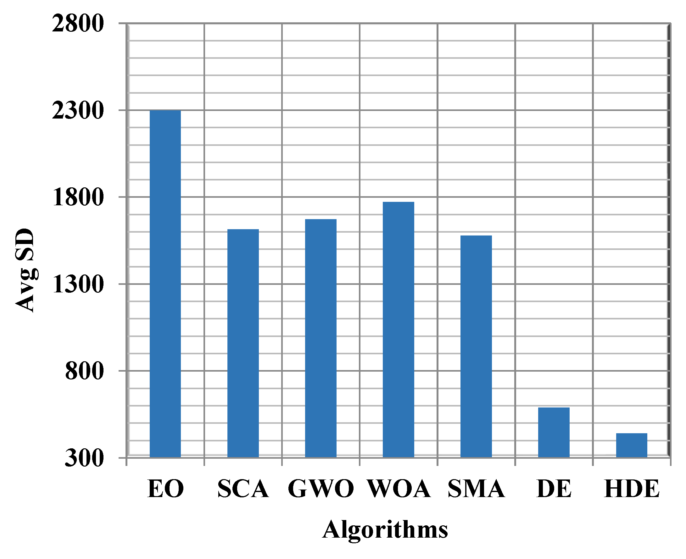
- The experimental findings show that HDE was the most effective metaheuristic scheduling algorithm among the compared approaches.
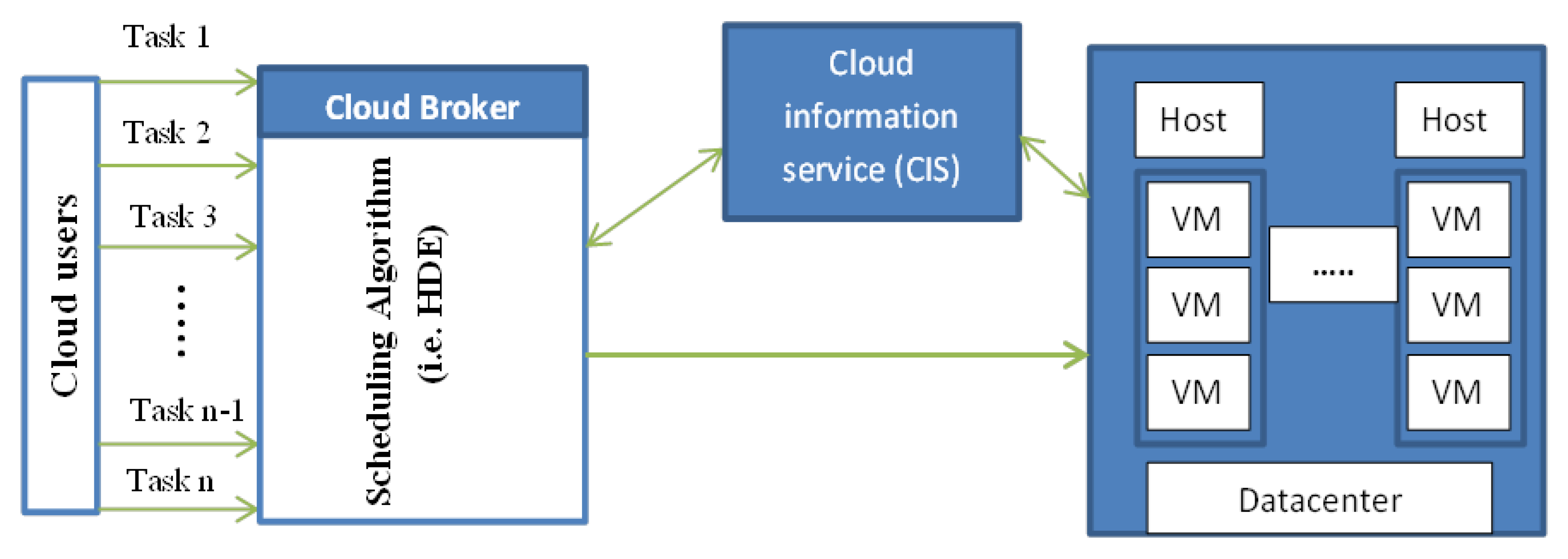
2. Task Scheduling in the Cloud Computing Environment
3. Differential Evolution
3.1. Mutation Operator
3.2. Crossover Operator
3.3. Selection Operator
4. Objective Function Formulation
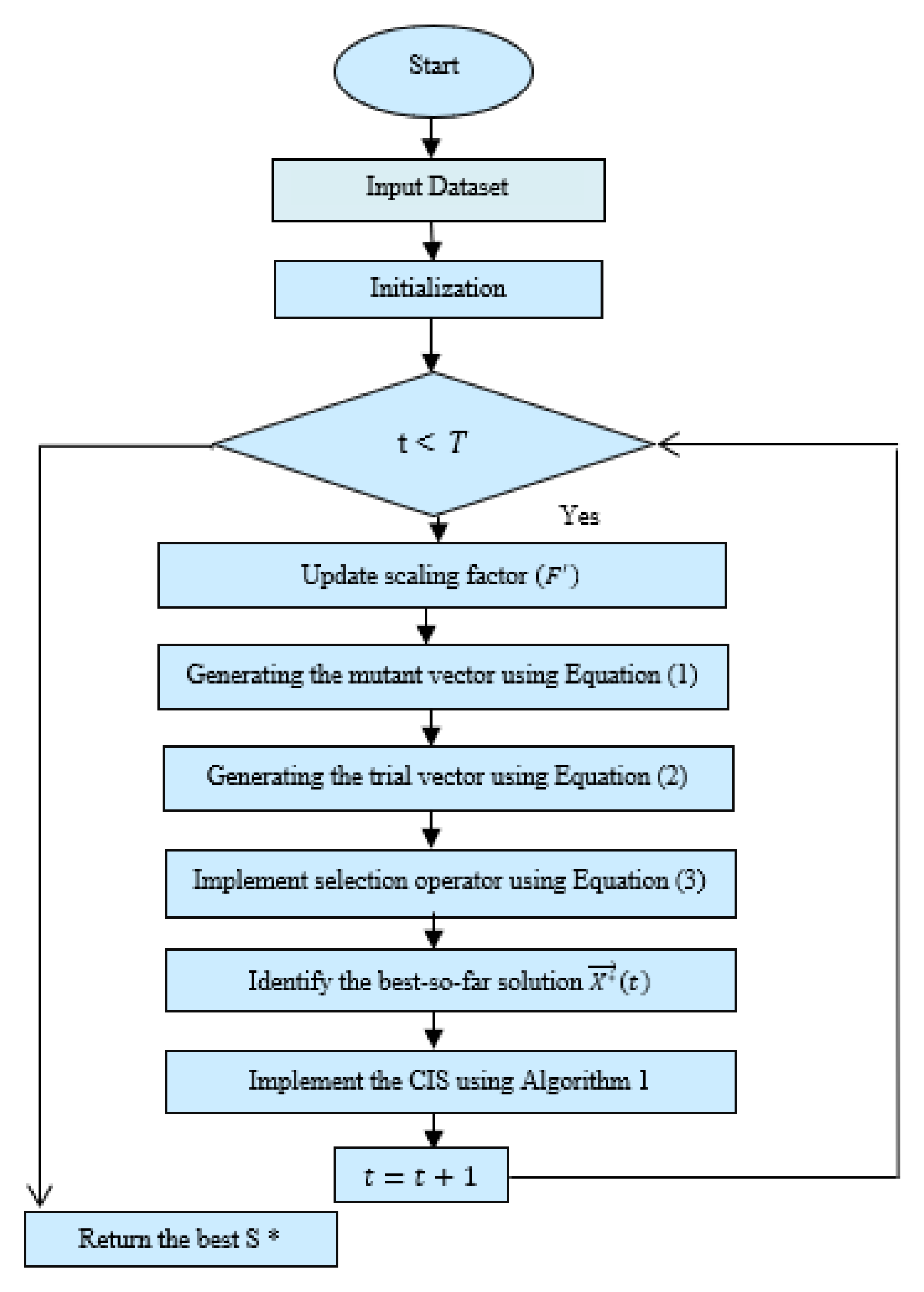
5. The Proposed Algorithm
5.1. Initialization
5.2. Adaptive Scaling Factor (F)
5.3. Convergence Improvement Strategy
| Algorithm 1. Convergence improvement strategy (CIS) |
| 1. for to 2. Generate the mutant vector using Equation (9) 3. for j = 0 to n 4. a number generated randomly between 0 and 1 5. ) 6. 7. else 8. 9. End if 10. end for 11. 12. = 13. end 14. Replace the best-so-far solution with if is better 15. end for |
5.4. Hybrid Differential Evolution
| Algorithm 2. Hybrid differential evolution (HDE) |
| 1. Initializes solutions, , using Equation (7) 2. Evaluate the initialized solutions and identified 3. 4. while (t < ) 5. Update using Equation (8) 6. 7. for to 8. Generate the mutant vector using Equation (1) 9. 10. for j = 0 to n 11. a number generated randomly between 0 and 1 12. ) 13. 14. else 15. 16. End if 17. end for 18. 19. = 20. end 21. Replace the best-so-far solution with if is better 22. end for 23. Updating solutions using the CIS algorithm (Algorithm 1) 24. 25. end while Return |
5.5. Time Complexity of HDE
6. Results and Simulation
6.1. Comparison with Metaheuristic Algorithms
6.2. Comparison with Some Heuristic Algorithms
6.3. Simulation Results
7. Conclusions and Future Work
Author Contributions
Funding
Data Availability Statement
Conflicts of Interest
Appendix A. Comparison with Some Heuristic and Metaheuristic Algorithms

| TS | EO | SCA | GWO | WOA | SMA | DE | HDE | |
|---|---|---|---|---|---|---|---|---|
| T100 | Best | 18,265.116 | 24,611.809 | 24,088.115 | 19,972.837 | 24,613.264 | 15,150.553 | 15,137.092 |
| Avg | 19,571.000 | 25,528.000 | 25,375.000 | 21,258.000 | 25,704.000 | 15,196.000 | 15,274.000 | |
| Worst | 21,498.010 | 26,402.739 | 26,051.051 | 22,205.813 | 26,752.888 | 15,257.978 | 15,558.919 | |
| SD | 713.524 | 463.258 | 424.731 | 558.666 | 521.104 | 30.572 | 91.663 | |
| T200 | Best | 42,426.362 | 48,950.808 | 49,292.426 | 42,546.316 | 49,025.035 | 29,373.841 | 28,909.445 |
| Avg | 44,394.000 | 50,538.000 | 50,422.000 | 44,527.000 | 50,967.000 | 29,627.000 | 29,231.000 | |
| Worst | 45,476.446 | 51,690.914 | 51,790.672 | 46,474.198 | 52,320.876 | 30,126.857 | 29,605.929 | |
| SD | 828.993 | 778.633 | 618.134 | 1021.092 | 811.779 | 184.835 | 184.273 | |
| T300 | Best | 69,067.191 | 74,866.300 | 74,062.850 | 66,476.677 | 75,546.109 | 46,803.516 | 43,810.658 |
| Avg | 71,383.000 | 76,534.000 | 77,081.000 | 69,943.000 | 76,864.000 | 47,615.000 | 44,284.000 | |
| Worst | 73,579.777 | 78,080.754 | 78,483.051 | 73,289.182 | 78,743.006 | 48,568.449 | 44,801.076 | |
| SD | 1134.455 | 867.221 | 1041.396 | 1443.511 | 874.786 | 430.618 | 255.008 | |
| T400 | Best | 95,440.911 | 98,432.590 | 99,668.262 | 92,093.906 | 99,673.090 | 64,938.822 | 58,147.125 |
| Avg | 98,176.000 | 102,045.000 | 102,211.000 | 94,585.000 | 102,252.000 | 66,478.000 | 58,708.000 | |
| Worst | 101,000.236 | 104,376.315 | 104,112.797 | 98,252.609 | 105,053.622 | 67,814.981 | 59,395.477 | |
| SD | 1348.619 | 1285.976 | 1075.139 | 1514.400 | 1256.732 | 701.588 | 323.410 | |
| T500 | Best | 120,119.573 | 123,408.542 | 123,758.958 | 115,201.767 | 125,660.988 | 84,738.675 | 72,282.977 |
| Avg | 123,307.000 | 127,282.000 | 127,133.000 | 119,111.000 | 127,791.000 | 86,195.000 | 73,084.000 | |
| Worst | 125,568.639 | 129,252.182 | 129,228.583 | 122,399.771 | 129,623.395 | 87,526.696 | 74,219.055 | |
| SD | 1440.633 | 1187.152 | 1291.705 | 1697.175 | 919.858 | 809.404 | 463.869 | |
| T600 | Best | 145,919.544 | 149,987.437 | 150,121.722 | 142,155.751 | 148,997.028 | 106,351.443 | 88,355.874 |
| Avg | 148,462.000 | 152,813.000 | 152,648.000 | 144,351.000 | 152,621.000 | 108,316.000 | 89,783.000 | |
| Worst | 151,270.871 | 155,095.573 | 154,638.766 | 146,586.770 | 155,053.210 | 110,123.047 | 91,415.701 | |
| SD | 1292.904 | 1264.745 | 1003.265 | 1346.239 | 1435.543 | 980.036 | 646.848 | |
| T700 | Best | 171,248.666 | 174,068.432 | 172,269.168 | 162,866.453 | 171,421.871 | 128,092.342 | 103,753.063 |
| Avg | 173,404.000 | 176,365.000 | 176,581.000 | 168,979.000 | 176,401.000 | 129,789.000 | 105,350.000 | |
| Worst | 177,380.381 | 178,450.265 | 180,508.600 | 174,375.747 | 179,642.085 | 131,573.149 | 107,198.432 | |
| SD | 1388.031 | 1166.368 | 1703.244 | 2689.929 | 1563.520 | 800.844 | 750.188 | |
| T800 | Best | 197,457.353 | 200,198.689 | 199,590.942 | 190,388.160 | 200,882.988 | 149,519.095 | 117,842.491 |
| Avg | 201,048.000 | 203,729.000 | 203,492.000 | 195,286.000 | 203,970.000 | 152,379.000 | 120,551.000 | |
| Worst | 204,902.594 | 206,534.694 | 207,776.148 | 200,825.073 | 206,878.190 | 154,292.126 | 123,731.662 | |
| SD | 1683.470 | 1656.565 | 1899.381 | 2196.411 | 1523.478 | 1199.194 | 1176.508 | |
| T900 | Best | 223,704.461 | 226,558.832 | 226,409.487 | 217,996.729 | 226,114.867 | 172,082.041 | 135,865.435 |
| Avg | 226,980.000 | 229,924.000 | 230,362.000 | 222,388.000 | 229,935.000 | 174,181.000 | 137,631.000 | |
| Worst | 229,921.195 | 233,724.590 | 233,488.493 | 225,639.051 | 233,651.341 | 176,793.002 | 139,246.915 | |
| SD | 1673.049 | 1834.109 | 1787.159 | 1794.545 | 1706.194 | 1229.686 | 863.086 | |
| T1000 | Best | 247,875.320 | 249,814.443 | 250,647.285 | 242,389.074 | 250,741.549 | 194,418.935 | 152,868.454 |
| Avg | 251,792.000 | 253,414.000 | 253,521.000 | 246,631.000 | 253,945.000 | 196,598.000 | 155,350.000 | |
| Worst | 254,529.450 | 257,498.878 | 256,169.629 | 250,551.728 | 256,575.530 | 198,807.888 | 157,666.486 | |
| SD | 1615.810 | 1823.711 | 1598.983 | 1604.413 | 1469.167 | 1146.393 | 1329.473 | |
| T1200 | Best | 272,161.798 | 275,012.674 | 273,177.920 | 266,930.950 | 275,918.637 | 215,439.409 | 168,684.208 |
| Avg | 276,665.000 | 278,762.000 | 278,623.000 | 272,150.000 | 279,459.000 | 218,984.000 | 172,241.000 | |
| Worst | 279,816.799 | 282,024.626 | 282,025.504 | 277,318.739 | 281,727.579 | 220,993.332 | 175,396.503 | |
| SD | 1654.505 | 1979.462 | 2136.547 | 2217.506 | 1530.659 | 1458.254 | 1543.670 | |
| T1500 | Best | 297,700.056 | 301,895.921 | 300,516.283 | 289,987.072 | 301,107.227 | 240,484.692 | 188,831.791 |
| Avg | 302,389.000 | 304,816.000 | 305,067.000 | 297,244.000 | 304,918.000 | 243,074.000 | 192,415.000 | |
| Worst | 306,262.646 | 306,790.966 | 307,331.538 | 300,181.346 | 308,731.491 | 245,362.366 | 195,299.922 | |
| SD | 2105.256 | 1457.285 | 1731.171 | 2124.410 | 1735.142 | 1424.956 | 1558.728 | |
| T2000 | Best | 324,305.532 | 328,468.897 | 328,886.931 | 318,205.762 | 325,580.330 | 265,211.125 | 209,699.639 |
| Avg | 329,160.000 | 331,652.000 | 331,396.000 | 323,903.000 | 330,530.000 | 268,229.000 | 212,927.000 | |
| Worst | 332,916.550 | 335,830.685 | 334,367.352 | 329,829.207 | 334,457.438 | 270,526.428 | 216,136.640 | |
| SD | 2167.010 | 1789.437 | 1634.825 | 2473.637 | 1970.316 | 1248.839 | 1521.468 | |
| T2500 | Best | 349,691.604 | 350,883.081 | 352,358.092 | 343,367.024 | 351,080.666 | 286,532.304 | 224,756.706 |
| Avg | 353,786.000 | 355,235.000 | 355,558.000 | 348,528.000 | 355,706.000 | 289,731.000 | 228,761.000 | |
| Worst | 357,011.837 | 359,479.690 | 358,061.266 | 352,923.652 | 360,249.932 | 292,567.734 | 233,007.159 | |
| SD | 1762.202 | 1972.154 | 1614.774 | 2190.929 | 2216.089 | 1639.396 | 1996.000 | |
| T3000 | Best | 374,687.613 | 374,116.100 | 378,044.013 | 368,165.769 | 374,348.289 | 308,332.567 | 247,888.247 |
| Avg | 380,344.000 | 382,277.000 | 382,538.000 | 375,197.000 | 381,730.000 | 314,351.000 | 250,242.000 | |
| Worst | 384,988.196 | 386,465.343 | 386,075.515 | 380,355.337 | 386,174.587 | 317,335.349 | 253,382.767 | |
| SD | 2444.072 | 2658.810 | 2068.051 | 2672.652 | 2505.108 | 2100.287 | 1509.886 |
| TS | EO | SCA | GWO | WOA | SMA | DE | HDE | |
|---|---|---|---|---|---|---|---|---|
| T100 | Best | 9438.672 | 11,947.637 | 12,712.777 | 10,884.463 | 11,975.781 | 6944.882 | 6944.882 |
| Avg | 10,516.000 | 12,859.000 | 13,645.000 | 11,750.000 | 12,807.000 | 7010.000 | 7013.000 | |
| Worst | 12,883.040 | 14,826.337 | 15,092.457 | 12,654.819 | 13,823.656 | 7137.436 | 7129.975 | |
| SD | 653.494 | 683.114 | 571.680 | 447.619 | 553.510 | 40.354 | 43.224 | |
| T200 | Best | 22,547.028 | 23,002.456 | 23,210.790 | 21,671.230 | 23,050.308 | 13,431.827 | 13,185.932 |
| Avg | 24,472.000 | 24,684.000 | 25,148.000 | 23,759.000 | 24,660.000 | 13,594.000 | 13,348.000 | |
| Worst | 26,066.689 | 26,378.086 | 27,355.248 | 25,403.570 | 26,345.011 | 14,041.473 | 13,538.203 | |
| SD | 829.519 | 960.601 | 1163.940 | 882.523 | 888.877 | 129.345 | 91.631 | |
| T300 | Best | 36,947.699 | 34,559.880 | 34,731.946 | 34,232.690 | 35,303.618 | 21,389.497 | 19,972.977 |
| Avg | 38,439.000 | 36,801.000 | 37,327.000 | 36,425.000 | 36,938.000 | 21,878.000 | 20,194.000 | |
| Worst | 40,431.356 | 38,900.228 | 41,404.623 | 39,453.807 | 39,017.019 | 22,363.346 | 20,472.578 | |
| SD | 976.881 | 909.559 | 1666.857 | 1116.936 | 854.587 | 228.565 | 127.459 | |
| T400 | Best | 48,955.367 | 45,647.852 | 46,915.152 | 46,597.809 | 46,455.141 | 29,617.292 | 26,444.417 |
| Avg | 51,779.000 | 48,799.000 | 48,556.000 | 48,947.000 | 48,528.000 | 30,500.000 | 26,731.000 | |
| Worst | 55,070.040 | 51,597.179 | 52,287.562 | 51,820.391 | 50,765.243 | 31,290.145 | 27,121.008 | |
| SD | 1509.922 | 1383.763 | 1272.435 | 1346.970 | 1208.233 | 400.760 | 161.878 | |
| T500 | Best | 61,001.750 | 57,658.760 | 57,566.241 | 58,607.792 | 59,016.133 | 38,674.036 | 32,957.020 |
| Avg | 64,916.000 | 60,584.000 | 60,244.000 | 60,900.000 | 60,608.000 | 39,487.000 | 33,269.000 | |
| Worst | 67,560.243 | 64,112.117 | 62,532.085 | 63,017.762 | 62,815.301 | 40,093.788 | 33,819.042 | |
| SD | 1560.291 | 1421.079 | 1234.821 | 1193.972 | 940.158 | 417.670 | 224.071 | |
| T600 | Best | 73,229.925 | 69,331.153 | 69,586.533 | 69,647.496 | 68,512.668 | 48,727.438 | 40,158.207 |
| Avg | 76,445.000 | 72,328.000 | 72,067.000 | 72,844.000 | 72,158.000 | 49,612.000 | 40,845.000 | |
| Worst | 80,532.895 | 77,530.876 | 75,054.437 | 77,227.793 | 749,26.269 | 50,879.790 | 41,495.153 | |
| SD | 1701.605 | 1594.430 | 1333.427 | 1659.749 | 1515.736 | 541.237 | 292.474 | |
| T700 | Best | 84,822.010 | 81,046.928 | 80,384.642 | 79,314.560 | 79,554.619 | 58,557.297 | 47,217.700 |
| Avg | 88,690.000 | 83,167.000 | 83,246.000 | 84,249.000 | 82,848.000 | 59,386.000 | 47,921.000 | |
| Worst | 93,188.460 | 85,347.315 | 86,615.127 | 87,747.237 | 86,999.870 | 60,544.019 | 48,675.067 | |
| SD | 2128.515 | 1231.305 | 1612.775 | 1790.731 | 1662.438 | 460.926 | 330.657 | |
| T800 | Best | 96,380.442 | 92,521.921 | 92,321.704 | 91,262.035 | 93,067.232 | 68,677.526 | 53,779.212 |
| Avg | 100,603.000 | 95,559.000 | 95,873.000 | 96,413.000 | 96,213.000 | 69,688.000 | 54,867.000 | |
| Worst | 106,564.905 | 98,404.951 | 99,524.222 | 100,831.242 | 101,401.679 | 70,661.792 | 56,282.630 | |
| SD | 2414.587 | 1423.826 | 2017.753 | 2166.084 | 2066.140 | 513.065 | 545.623 | |
| T900 | Best | 108,229.730 | 103,645.560 | 104,628.113 | 105,548.365 | 104,277.133 | 78,792.104 | 61,758.499 |
| Avg | 113,582.000 | 107,669.000 | 107,999.000 | 109,495.000 | 107,688.000 | 79,775.000 | 62,626.000 | |
| Worst | 120,148.440 | 112,419.694 | 114,072.174 | 111,749.833 | 111,998.498 | 81,359.462 | 63,399.167 | |
| SD | 2850.589 | 2007.737 | 2051.189 | 1641.801 | 1715.424 | 624.858 | 408.529 | |
| T1000 | Best | 118,736.975 | 115,138.440 | 115,625.172 | 116,100.770 | 116,206.118 | 88,832.449 | 69,515.446 |
| Avg | 123,279.000 | 118,956.000 | 119,125.000 | 120,234.000 | 118,929.000 | 90,012.000 | 70,684.000 | |
| Worst | 129,183.176 | 122,706.004 | 122,156.907 | 124,499.643 | 124,431.728 | 93,798.984 | 71,658.817 | |
| SD | 2489.881 | 1666.849 | 1659.843 | 2417.331 | 1778.316 | 874.974 | 620.257 | |
| T1200 | Best | 129,795.983 | 126,954.152 | 126,249.252 | 127,570.871 | 127,972.633 | 98,118.160 | 76,652.611 |
| Avg | 134,908.000 | 130,688.000 | 130,519.000 | 132,035.000 | 130,779.000 | 100,158.000 | 78,409.000 | |
| Worst | 141,397.459 | 135,719.950 | 134,650.907 | 139,766.474 | 136,984.431 | 101,266.796 | 79,725.686 | |
| SD | 2309.279 | 1870.231 | 2018.753 | 2729.933 | 2251.355 | 774.466 | 705.732 | |
| T1500 | Best | 138,804.579 | 138,898.602 | 139,292.203 | 139,693.196 | 138,606.731 | 109,581.936 | 85,953.213 |
| Avg | 145,796.000 | 142,250.000 | 142,775.000 | 143,012.000 | 142,380.000 | 111,340.000 | 87,520.000 | |
| Worst | 153,587.370 | 145,607.443 | 150,992.953 | 147,576.341 | 146,704.239 | 114,272.274 | 89,009.316 | |
| SD | 3283.758 | 1526.583 | 2390.077 | 1991.793 | 1614.124 | 1072.070 | 721.108 | |
| T2000 | Best | 151,784.006 | 151,264.096 | 150,594.060 | 149,722.432 | 151,191.472 | 121,190.063 | 95,349.975 |
| Avg | 157,611.000 | 155,420.000 | 154,648.000 | 155,396.000 | 154,322.000 | 122,618.000 | 96,813.000 | |
| Worst | 166,344.617 | 160,214.293 | 159,508.888 | 161,005.512 | 159,349.068 | 123,936.506 | 98,162.927 | |
| SD | 3677.971 | 2504.031 | 2137.704 | 2628.660 | 1852.858 | 637.741 | 698.603 | |
| T2500 | Best | 160,529.235 | 160,637.179 | 162,072.574 | 161,144.576 | 161,100.021 | 130,477.400 | 102,136.632 |
| Avg | 169,506.000 | 165,738.000 | 166,038.000 | 166,450.000 | 165,581.000 | 132,810.000 | 104,022.000 | |
| Worst | 179,163.135 | 171,771.518 | 169,385.501 | 173,371.558 | 169,513.351 | 134,690.256 | 106,190.281 | |
| SD | 4406.047 | 2343.341 | 1588.846 | 2503.864 | 2282.155 | 925.081 | 933.183 | |
| T3000 | Best | 172,070.805 | 172,887.505 | 173,311.921 | 174,193.094 | 173,026.585 | 142,122.392 | 112,625.384 |
| Avg | 181,066.000 | 177,940.000 | 178,119.000 | 178,707.000 | 177,882.000 | 144,111.000 | 113,811.000 | |
| Worst | 187,904.224 | 184,878.509 | 182,574.837 | 183,514.827 | 181,860.483 | 147,212.405 | 115,274.338 | |
| SD | 3690.548 | 2693.045 | 2364.794 | 2069.685 | 2493.556 | 1188.774 | 701.579 |
| TS | EO | SCA | GWO | WOA | SMA | DE | HDE | |
|---|---|---|---|---|---|---|---|---|
| T100 | Best | 38,115.003 | 50,570.643 | 49,339.028 | 40,070.182 | 52,314.209 | 34,167.699 | 34,184.939 |
| Avg | 40,701.000 | 55,087.000 | 52,746.000 | 43,443.000 | 55,795.000 | 34,298.000 | 34,550.000 | |
| Worst | 43,980.020 | 57,190.514 | 56,010.407 | 46,197.991 | 57,836.610 | 34,461.035 | 35,226.454 | |
| SD | 1093.390 | 1509.796 | 1560.900 | 1514.701 | 1342.057 | 74.832 | 228.008 | |
| T200 | Best | 86,987.143 | 105,072.258 | 103,976.815 | 87,848.691 | 108,440.506 | 66,302.970 | 65,521.241 |
| Avg | 90,879.000 | 110,862.000 | 109,394.000 | 92,988.000 | 112,350.000 | 67,038.000 | 66,290.000 | |
| Worst | 95,059.361 | 114,933.861 | 113,761.796 | 98,376.422 | 115,141.894 | 67,843.837 | 67,119.554 | |
| SD | 2114.152 | 2408.720 | 2660.714 | 2577.679 | 1907.367 | 414.783 | 429.283 | |
| T300 | Best | 140,739.328 | 164,556.186 | 161,414.947 | 141,130.001 | 165,788.713 | 105,870.995 | 99,269.263 |
| Avg | 148,252.000 | 169,244.000 | 169,843.000 | 148,151.000 | 170,026.000 | 107,669.000 | 100,496.000 | |
| Worst | 151,986.556 | 172,666.021 | 175,454.835 | 155,885.560 | 174,514.307 | 109,713.690 | 101,829.995 | |
| SD | 2883.541 | 1929.747 | 3292.297 | 3351.197 | 2029.973 | 1011.817 | 610.498 | |
| T400 | Best | 197,268.901 | 220,893.125 | 220,314.876 | 194,313.759 | 223,848.304 | 146,681.999 | 132,120.112 |
| Avg | 206,434.000 | 226,286.000 | 227,406.000 | 201,072.000 | 227,607.000 | 150,428.000 | 133,321.000 | |
| Worst | 212,775.565 | 233,178.780 | 233,772.309 | 213,052.367 | 234,076.000 | 153,333.362 | 134,949.635 | |
| SD | 3429.782 | 2590.382 | 2766.779 | 4734.105 | 2765.688 | 1528.621 | 718.928 | |
| T500 | Best | 250,376.325 | 276,708.351 | 275,486.339 | 245,134.200 | 28,0346.649 | 191,901.169 | 164,043.543 |
| Avg | 259,553.000 | 282,911.000 | 283,207.000 | 254,935.000 | 284,552.000 | 195,182.000 | 165,984.000 | |
| Worst | 268,501.754 | 288,230.427 | 288,712.693 | 264,972.627 | 289,984.941 | 198,374.617 | 168,523.978 | |
| SD | 4225.905 | 2899.368 | 3376.512 | 4857.550 | 2312.076 | 1837.159 | 1043.599 | |
| T600 | Best | 305,869.915 | 333,578.543 | 335,046.072 | 298,840.145 | 331,419.196 | 240,743.608 | 200,817.097 |
| Avg | 316,503.000 | 340,612.000 | 340,669.000 | 311,202.000 | 340,368.000 | 245,292.000 | 203,972.000 | |
| Worst | 322,769.104 | 345,645.788 | 346,242.900 | 320,955.422 | 346,933.177 | 249,268.571 | 207,896.980 | |
| SD | 4545.269 | 2832.242 | 2863.235 | 4729.092 | 3649.364 | 2146.239 | 1492.645 | |
| T700 | Best | 357,976.309 | 386,497.338 | 386,666.396 | 348,756.713 | 384,774.422 | 290,119.422 | 235,668.911 |
| Avg | 371,070.000 | 393,829.000 | 394,363.000 | 366,683.000 | 394,693.000 | 294,062.000 | 239,351.000 | |
| Worst | 378,442.442 | 401,305.913 | 400,091.078 | 380,151.696 | 402,525.765 | 297,527.211 | 243,753.678 | |
| SD | 4873.732 | 3716.885 | 3533.207 | 8468.329 | 3321.936 | 1805.772 | 1741.489 | |
| T800 | Best | 426,788.885 | 443,078.326 | 445,461.575 | 413,981.425 | 446,848.296 | 337,406.050 | 267,323.474 |
| Avg | 435,421.000 | 456,128.000 | 454,603.000 | 425,991.000 | 455,402.000 | 345,326.000 | 273,815.000 | |
| Worst | 447,835.415 | 462,814.404 | 465,671.838 | 440,590.901 | 462,478.406 | 350,468.826 | 281,112.735 | |
| SD | 5155.694 | 4975.650 | 4760.611 | 6537.117 | 3175.612 | 3129.091 | 2672.983 | |
| T900 | Best | 477,747.825 | 508,820.405 | 507,406.435 | 474,814.038 | 505,128.246 | 388,859.617 | 308,781.618 |
| Avg | 491,572.000 | 515,186.000 | 515,877.000 | 485,805.000 | 515,177.000 | 394,463.000 | 312,644.000 | |
| Worst | 500,984.743 | 522,422.130 | 524,740.549 | 497,009.192 | 523,713.793 | 401,004.355 | 316,484.309 | |
| SD | 5365.567 | 3128.123 | 4096.034 | 5414.481 | 4544.028 | 3238.249 | 1943.345 | |
| T1000 | Best | 537,828.097 | 557,237.156 | 556,031.484 | 524,852.018 | 558,305.219 | 439,473.809 | 347,358.806 |
| Avg | 551,656.000 | 567,151.000 | 567,112.000 | 541,558.000 | 568,982.000 | 445,298.000 | 352,903.000 | |
| Worst | 563,670.866 | 575,833.134 | 574,415.860 | 553,355.183 | 575,042.293 | 451,669.178 | 358,351.049 | |
| SD | 6829.226 | 4411.820 | 4635.891 | 6413.167 | 3339.505 | 2816.904 | 3011.747 | |
| T1200 | Best | 588,406.658 | 616,501.616 | 609,146.791 | 585,013.689 | 612,946.921 | 489,188.988 | 383,424.603 |
| Avg | 607,433.000 | 624,268.000 | 624,202.000 | 599,085.000 | 626,378.000 | 496,245.000 | 391,183.000 | |
| Worst | 621,660.221 | 633,980.837 | 632,138.961 | 612,439.335 | 634,727.265 | 501,846.993 | 398,628.411 | |
| SD | 6446.235 | 4055.883 | 5021.459 | 7582.436 | 5868.540 | 3414.373 | 3541.414 | |
| T1500 | Best | 645,910.065 | 678,355.899 | 671,733.428 | 640,448.075 | 677,639.783 | 545,069.758 | 428,881.806 |
| Avg | 667,774.000 | 684,136.000 | 683,749.000 | 657,119.000 | 684,171.000 | 550,454.000 | 437,170.000 | |
| Worst | 690,938.157 | 694,111.491 | 693,117.184 | 666,430.377 | 695,449.033 | 556,975.679 | 443,311.339 | |
| SD | 8351.155 | 3736.241 | 5531.450 | 6816.146 | 4114.685 | 3010.062 | 3530.292 | |
| T2000 | Best | 712,207.300 | 733,380.764 | 737,130.722 | 702,518.639 | 731,200.908 | 599,158.246 | 476,515.523 |
| Avg | 729,441.000 | 742,861.000 | 743,809.000 | 717,086.000 | 741,682.000 | 607,988.000 | 483,857.000 | |
| Worst | 741,210.983 | 752,039.100 | 753,733.583 | 730,721.668 | 749,436.738 | 613,091.297 | 491,408.639 | |
| SD | 6883.118 | 4637.338 | 4247.121 | 6992.119 | 4927.330 | 3101.014 | 3462.359 | |
| T2500 | Best | 765,728.675 | 787,262.395 | 785,012.916 | 755,291.076 | 791,036.794 | 646,478.360 | 510,870.211 |
| Avg | 783,772.000 | 797,394.000 | 797,769.000 | 773,376.000 | 799,331.000 | 655,880.000 | 519,819.000 | |
| Worst | 796,845.810 | 805,270.438 | 809,131.565 | 789,947.532 | 808,619.056 | 661,680.775 | 528,913.206 | |
| SD | 7897.303 | 4431.070 | 5327.938 | 8487.814 | 4819.742 | 3862.820 | 4496.779 | |
| T3000 | Best | 830,030.908 | 843,649.488 | 851,616.785 | 810,725.718 | 843,766.365 | 696,078.733 | 563,250.918 |
| Avg | 845,325.000 | 859,065.000 | 859,517.000 | 833,672.000 | 857,376.000 | 711,579.000 | 568,580.000 | |
| Worst | 860,345.325 | 868,701.031 | 866,711.674 | 846,150.448 | 867,698.102 | 718,347.423 | 575,635.766 | |
| SD | 7084.137 | 5029.439 | 3972.881 | 8360.492 | 5830.941 | 5256.236 | 3441.967 |
| TS | EO | SCA | GWO | WOA | SMA | DE | |
|---|---|---|---|---|---|---|---|
| T100 | h- | 3.01986 × 10⁻¹¹ | 3.01986 × 10⁻¹¹ | 3.01986 × 10⁻¹¹ | 3.01986 × 10⁻¹¹ | 3.01986 × 10⁻¹¹ | 6.35455 × 10⁻⁵ |
| p- | 1 | 1 | 1 | 1 | 1 | 1 | |
| T200 | h- | 3.01986 × 10⁻¹¹ | 3.01986 × 10⁻¹¹ | 3.01986 × 10⁻¹¹ | 3.01986 × 10⁻¹¹ | 3.01986 × 10⁻¹¹ | 7.77255 × 10⁻⁹ |
| p- | 1 | 1 | 1 | 1 | 1 | 1 | |
| T300 | h- | 3.01986 × 10⁻¹¹ | 3.01986 × 10⁻¹¹ | 3.01986 × 10⁻¹¹ | 3.01986 × 10⁻¹¹ | 3.01986 × 10⁻¹¹ | 3.01986 × 10⁻¹¹ |
| p- | 1 | 1 | 1 | 1 | 1 | 1 | |
| T400 | h- | 3.01986 × 10⁻¹¹ | 3.01986 × 10⁻¹¹ | 3.01986 × 10⁻¹¹ | 3.01986 × 10⁻¹¹ | 3.01986 × 10⁻¹¹ | 3.01986 × 10⁻¹¹ |
| p- | 1 | 1 | 1 | 1 | 1 | 1 | |
| T500 | h- | 3.01986 × 10⁻¹¹ | 3.01986 × 10⁻¹¹ | 3.01986 × 10⁻¹¹ | 3.01986 × 10⁻¹¹ | 3.01986 × 10⁻¹¹ | 3.01986 × 10⁻¹¹ |
| p- | 1 | 1 | 1 | 1 | 1 | 1 | |
| T600 | h- | 3.01986 × 10⁻¹¹ | 3.01986 × 10⁻¹¹ | 3.01986 × 10⁻¹¹ | 3.01986 × 10⁻¹¹ | 3.01986 × 10⁻¹¹ | 3.01986 × 10⁻¹¹ |
| p- | 1 | 1 | 1 | 1 | 1 | 1 | |
| T700 | h- | 3.01986 × 10⁻¹¹ | 3.01986 × 10⁻¹¹ | 3.01986 × 10⁻¹¹ | 3.01986 × 10⁻¹¹ | 3.01986 × 10⁻¹¹ | 3.01986 × 10⁻¹¹ |
| p- | 1 | 1 | 1 | 1 | 1 | 1 | |
| T800 | h- | 3.01986 × 10⁻¹¹ | 3.01986 × 10⁻¹¹ | 3.01986 × 10⁻¹¹ | 3.01986 × 10⁻¹¹ | 3.01986 × 10⁻¹¹ | 3.01986 × 10⁻¹¹ |
| p- | 1 | 1 | 1 | 1 | 1 | 1 | |
| T900 | h- | 3.01986 × 10⁻¹¹ | 3.01986 × 10⁻¹¹ | 3.01986 × 10⁻¹¹ | 3.01986 × 10⁻¹¹ | 3.01986 × 10⁻¹¹ | 3.01986 × 10⁻¹¹ |
| p- | 1 | 1 | 1 | 1 | 1 | 1 | |
| T1000 | h- | 3.01986 × 10⁻¹¹ | 3.01986 × 10⁻¹¹ | 3.01986 × 10⁻¹¹ | 3.01986 × 10⁻¹¹ | 3.01986 × 10⁻¹¹ | 3.01986 × 10⁻¹¹ |
| p- | 1 | 1 | 1 | 1 | 1 | 1 |
| FCFS | SJF | RR | HDE | ||||||
|---|---|---|---|---|---|---|---|---|---|
| TS | MS | Total Execution | MS | Total Execution | MS | Total Execution | MS | Total Execution | |
| T100 | Best | 12,344.292 | 53,662.706 | 12,398.820 | 55,392.648 | 13,303.341 | 55,738.997 | 6944.882 | 34,184.939 |
| Avg | 14,910.000 | 58,624.000 | 14,562.000 | 59,537.000 | 15,390.000 | 59,010.000 | 7013.000 | 34,550.000 | |
| Worst | 17,044.315 | 62,160.312 | 18,442.821 | 64,955.074 | 20,028.542 | 62,707.336 | 7129.975 | 35,226.454 | |
| SD | 1285.666 | 2349.561 | 1369.898 | 2201.344 | 1582.706 | 1824.601 | 43.224 | 228.008 | |
| T200 | Best | 22,844.658 | 110,292.306 | 24,328.549 | 112,870.669 | 24,911.324 | 111,094.478 | 13,185.932 | 65,521.241 |
| Avg | 27,145.000 | 115,596.000 | 28,231.000 | 117,153.000 | 27,956.000 | 117,593.000 | 13,348.000 | 66,290.000 | |
| Worst | 31,734.097 | 121,304.186 | 33,372.631 | 124,674.725 | 30,746.313 | 122,266.950 | 13,538.203 | 67,119.554 | |
| SD | 1896.645 | 2616.447 | 2440.761 | 2513.921 | 1461.083 | 2916.001 | 91.631 | 429.283 | |
| T300 | Best | 36,401.175 | 167,860.710 | 35,551.337 | 169,794.780 | 37,405.544 | 170,045.361 | 19,972.977 | 99,269.263 |
| Avg | 40,855.000 | 174,596.000 | 40,437.000 | 175,831.000 | 40,835.000 | 174,987.000 | 20,194.000 | 100,496.000 | |
| Worst | 48,259.582 | 181,227.236 | 46,488.415 | 184,826.161 | 45,607.496 | 182,173.616 | 20,472.578 | 101,829.995 | |
| SD | 3164.196 | 3007.580 | 2540.009 | 3417.183 | 2145.982 | 2568.089 | 127.459 | 610.498 | |
| T400 | Best | 48,561.026 | 222,538.649 | 47,999.873 | 226,957.706 | 47,704.192 | 223,741.723 | 26,444.417 | 132,120.112 |
| Avg | 53,428.000 | 233,554.000 | 53,169.000 | 233,803.000 | 52,562.000 | 232,425.000 | 26,731.000 | 133,321.000 | |
| Worst | 61,278.109 | 246,043.696 | 61,410.113 | 241,419.656 | 56,838.183 | 240,902.340 | 27,121.008 | 134949.635 | |
| SD | 3014.512 | 4164.430 | 2703.758 | 3817.347 | 2201.783 | 4461.438 | 161.878 | 718.928 | |
| T500 | Best | 60,671.925 | 284,463.880 | 60,666.928 | 282,672.617 | 61,382.773 | 283,534.055 | 32,957.020 | 164,043.543 |
| Avg | 65,297.000 | 291,399.000 | 66,204.000 | 291,909.000 | 65,410.000 | 291,712.000 | 33,269.000 | 165,984.000 | |
| Worst | 73,599.101 | 301,398.628 | 76,683.101 | 300,649.387 | 74,272.381 | 297,917.527 | 33,819.042 | 168,523.978 | |
| SD | 3065.808 | 3745.909 | 4217.987 | 4207.052 | 3169.840 | 2995.869 | 224.071 | 1043.599 | |
| T600 | Best | 71,384.337 | 338,853.354 | 71,876.123 | 339,199.141 | 72,118.680 | 338,253.551 | 40,158.207 | 200,817.097 |
| Avg | 77,058.000 | 348,454.000 | 78,169.000 | 347,967.000 | 77,937.000 | 347189.000 | 40,845.000 | 203,972.000 | |
| Worst | 83,617.806 | 361,268.968 | 91,370.647 | 360,625.466 | 86,283.611 | 353,966.290 | 41,495.153 | 207,896.980 | |
| SD | 3655.534 | 5785.572 | 4347.694 | 5222.763 | 3596.340 | 3873.134 | 292.474 | 1492.645 | |
| T700 | Best | 82,871.222 | 389,875.874 | 83,096.043 | 393,296.088 | 81,664.036 | 394,618.246 | 47,217.700 | 235,668.911 |
| Avg | 88,977.000 | 403,648.000 | 88,430.000 | 402,422.000 | 89,694.000 | 404,010.000 | 47,921.000 | 239,351.000 | |
| Worst | 101,824.324 | 415,541.874 | 97,387.359 | 412,616.229 | 100,040.623 | 421,919.793 | 48,675.067 | 243,753.678 | |
| SD | 3883.562 | 6357.864 | 3321.412 | 4165.120 | 4360.224 | 5737.322 | 330.657 | 1741.489 | |
| T800 | Best | 95,526.392 | 451,999.107 | 95,363.041 | 449,490.324 | 92,544.224 | 449,997.947 | 53,779.212 | 267,323.474 |
| Avg | 102,116.000 | 464,544.000 | 101,688.000 | 464,338.000 | 102,840.000 | 463,833.000 | 54,867.000 | 273,815.000 | |
| Worst | 110,433.706 | 473,190.025 | 113,090.328 | 473,467.814 | 114,386.119 | 475,437.101 | 56,282.630 | 281,112.735 | |
| SD | 3423.486 | 4557.432 | 4046.083 | 5894.821 | 4732.558 | 6066.622 | 545.623 | 2672.983 | |
| T900 | Best | 108,219.570 | 507,238.701 | 106,632.715 | 512,446.913 | 107,182.309 | 512,662.893 | 61,758.499 | 308,781.618 |
| Avg | 113,943.000 | 524,054.000 | 114,563.000 | 523,459.000 | 114,571.000 | 524,364.000 | 62626.000 | 312,644.000 | |
| Worst | 122,612.509 | 542,323.705 | 126,840.703 | 539,681.496 | 123,633.119 | 538,450.021 | 63,399.167 | 316,484.309 | |
| SD | 4002.028 | 6410.736 | 4548.561 | 6594.319 | 4337.906 | 5915.235 | 408.529 | 1943.345 | |
| T1000 | Best | 115,252.394 | 562,357.362 | 115,970.112 | 563,944.718 | 117,570.996 | 564,348.540 | 69,515.446 | 347,358.806 |
| Avg | 123,900.000 | 575,167.000 | 124,553.000 | 577018.000 | 124,977.000 | 576,748.000 | 70,684.000 | 352,903.000 | |
| Worst | 132,163.539 | 584,019.817 | 139,114.933 | 594,497.693 | 134,407.616 | 590,320.838 | 71,658.817 | 358,351.049 | |
| SD | 3776.393 | 5114.537 | 4821.304 | 6486.320 | 4500.341 | 5778.815 | 620.257 | 3011.747 | |
| T1200 | Best | 126,473.499 | 622,184.636 | 128,882.364 | 619,891.703 | 129,100.117 | 620,290.715 | 76,652.611 | 383,424.603 |
| Avg | 137,267.000 | 637,357.000 | 137,832.000 | 636,864.000 | 136,112.000 | 634,428.000 | 78,409.000 | 391,183.000 | |
| Worst | 148,752.105 | 656,539.187 | 150,051.311 | 650,397.990 | 143,371.287 | 647,445.075 | 79,725.686 | 398,628.411 | |
| SD | 4887.727 | 8273.490 | 4775.503 | 6534.292 | 3190.396 | 6837.603 | 705.732 | 3541.414 | |
| T1500 | Best | 138,646.670 | 679,212.397 | 142,046.487 | 679,305.037 | 145,002.492 | 684,350.824 | 85,953.213 | 428,881.806 |
| Avg | 149,618.000 | 693,741.000 | 150,234.000 | 695,673.000 | 151,079.000 | 696,135.000 | 87,520.000 | 437,170.000 | |
| Worst | 165,002.833 | 707,135.205 | 164,234.551 | 708,533.638 | 160,514.410 | 708,776.628 | 89,009.316 | 443,311.339 | |
| SD | 6078.265 | 7948.496 | 5151.143 | 7429.044 | 4560.286 | 5537.040 | 721.108 | 3530.292 | |
| T2000 | Best | 153,066.964 | 737,643.035 | 153,299.956 | 734,958.438 | 152,479.492 | 740,924.563 | 95,349.975 | 476,515.523 |
| Avg | 161,641.000 | 754,762.000 | 162,568.000 | 754,581.000 | 159,989.000 | 752,314.000 | 96,813.000 | 483,857.000 | |
| Worst | 175,933.006 | 763,273.414 | 184,308.530 | 766,039.466 | 170,141.689 | 770,347.951 | 98,162.927 | 491,408.639 | |
| SD | 5660.829 | 6387.341 | 5766.332 | 7228.589 | 4479.952 | 7333.449 | 698.603 | 3462.359 | |
| T2500 | Best | 161,397.176 | 794,939.206 | 165,571.473 | 792,458.130 | 166,885.056 | 799,726.645 | 102,136.632 | 510,870.211 |
| Avg | 173,614.000 | 809,173.000 | 172,776.000 | 810,402.000 | 174375.000 | 812,225.000 | 104,022.000 | 519,819.000 | |
| Worst | 184,331.464 | 824,648.829 | 183,006.363 | 827,132.424 | 189,002.607 | 824,028.335 | 106,190.281 | 528,913.206 | |
| SD | 5457.343 | 7346.403 | 4412.046 | 7584.300 | 5523.036 | 6417.060 | 933.183 | 4496.779 | |
| T3000 | Best | 176,200.277 | 852,165.434 | 177,661.627 | 853,232.663 | 178,819.097 | 859,423.967 | 112,625.384 | 563,250.918 |
| Avg | 184,378.000 | 866,586.000 | 186,939.000 | 871,015.000 | 186,791.000 | 872,513.000 | 113,811.000 | 568,580.000 | |
| Worst | 196,778.207 | 885,253.124 | 201,877.303 | 892,941.694 | 201,607.603 | 888,088.876 | 115,274.338 | 575,635.766 | |
| SD | 5833.666 | 7420.404 | 5587.624 | 9231.738 | 6381.138 | 7657.639 | 701.579 | 3441.967 | |
References
- El-Shafeiy, E.; Abohany, A. A new swarm intelligence framework for the Internet of Medical Things system in healthcare. In Swarm Intelligence for Resource Management in Internet of Things; Academic Press: Cambridge, MA, USA, 2020; pp. 87–107. [Google Scholar] [CrossRef]
- Hassan, K.M.; Abdo, A.; Yakoub, A. Enhancement of Health Care Services based on cloud computing in IOT Environment Using Hybrid Swarm Intelligence. IEEE Access 2022, 10, 105877–105886. [Google Scholar] [CrossRef]
- Nayar, N.; Ahuja, S.; Jain, S. Swarm intelligence and data mining: A review of literature and applications in healthcare. In Proceedings of the Third International Conference on Advanced Informatics for Computing Research, Shimla, India, 15–16 June 2019. [Google Scholar]
- Ben Alla, H.; Ben Alla, S.; Touhafi, A.; Ezzati, A. A novel task scheduling approach based on dynamic queues and hybrid meta-heuristic algorithms for cloud computing environment. Clust. Comput. 2018, 21, 1797–1820. [Google Scholar] [CrossRef]
- Singh, H.; Tyagi, S.; Kumar, P.; Gill, S.S.; Buyya, R. Metaheuristics for scheduling of heterogeneous tasks in cloud computing environments: Analysis, performance evaluation, and future directions. Simul. Model. Pr. Theory 2021, 111, 102353. [Google Scholar] [CrossRef]
- Huang, X.; Li, C.; Chen, H.; An, D. Task scheduling in cloud computing using particle swarm optimization with time varying inertia weight strategies. Clust. Comput. 2020, 23, 1137–1147. [Google Scholar] [CrossRef]
- Bezdan, T.; Zivkovic, M.; Antonijevic, M.; Zivkovic, T.; Bacanin, N. Enhanced Flower Pollination Algorithm for Task Scheduling in Cloud Computing Environment. In Machine Learning for Predictive Analysis; Springer: Berlin/Heidelberg, Germany, 2021; pp. 163–171. [Google Scholar] [CrossRef]
- Choudhary, A.; Gupta, I.; Singh, V.; Jana, P.K. A GSA based hybrid algorithm for bi-objective workflow scheduling in cloud computing. Futur. Gener. Comput. Syst. 2018, 83, 14–26. [Google Scholar] [CrossRef]
- Raghavan, S.; Sarwesh, P.; Marimuthu, C.; Chandrasekaran, K. Bat algorithm for scheduling workflow applications in cloud. In Proceedings of the 2015 International Conference on Electronic Design, Computer Networks & Automated Verification (EDCAV), Shillon, India, 29–30 January 2015; pp. 139–144. [Google Scholar]
- Tawfeek, M.A.; El-Sisi, A.; Keshk, A.E.; Torkey, F.A. Cloud task scheduling based on ant colony optimization. In Proceedings of the 8th International Conference on Computer Engineering & Systems (ICCES), Cairo, Egypt, 26–28 November 2013; IEEE: Piscataway, NJ, USA, 2013. [Google Scholar]
- Hamad, S.A.; Omara, F.A. Genetic-Based Task Scheduling Algorithm in Cloud Computing Environment. Int. J. Adv. Comput. Sci. Appl. 2016, 7, 550–556. [Google Scholar] [CrossRef] [Green Version]
- Bacanin, N.; Bezdan, T.; Tuba, E.; Strumberger, I.; Tuba, M.; Zivkovic, M. Task Scheduling in Cloud Computing Environment by Grey Wolf Optimizer. In Proceedings of the 27th Telecommunications Forum (TELFOR), Belgrade, Serbia, 26–27 November 2019; pp. 1–4. [Google Scholar] [CrossRef]
- Chen, X.; Cheng, L.; Liu, C.; Liu, Q.; Liu, J.; Mao, Y.; Murphy, J. A WOA-Based Optimization Approach for Task Scheduling in Cloud Computing Systems. IEEE Syst. J. 2020, 14, 3117–3128. [Google Scholar] [CrossRef]
- Alsaidy, S.A.; Abbood, A.D.; Sahib, M.A. Heuristic initialization of PSO task scheduling algorithm in cloud computing. J. King Saud Univ. Comput. Inf. Sci. 2020, 34, 2370–2382. [Google Scholar] [CrossRef]
- Alboaneen, D.A.; Tianfield, H.; Zhang, Y. Glowworm swarm optimisation based task scheduling for cloud computing. In Proceedings of the Second International Conference on Internet of Things, Data and Cloud Computing, Porto, Portugal, 24–26 April 2017. [Google Scholar]
- Durgadevi, P.; Srinivasan, D.S. Task scheduling using amalgamation of metaheuristics swarm optimization algorithm and cuckoo search in cloud computing environment. J. Res. 2015, 1, 10–17. [Google Scholar]
- Belgacem, A.; Beghdad-Bey, K.; Nacer, H. Task scheduling optimization in cloud based on electromagnetism metaheuristic algorithm. In Proceedings of the 3rd International Conference on Pattern Analysis and Intelligent Systems (PAIS), Tebessa, Algeria, 24–25 October 2018; pp. 1–7. [Google Scholar] [CrossRef]
- Masadeh, R.; Alsharman, N.; Sharieh, A.; Mahafzah, B.; Abdulrahman, A. Task scheduling on cloud computing based on sea lion optimization algorithm. Int. J. Web Inf. Syst. 2021, 17, 99–116. [Google Scholar] [CrossRef]
- Abdullahi, M.; Ngadi, A.; Dishing, S.I.; Abdulhamid, S.M. An adaptive symbiotic organisms search for constrained task scheduling in cloud computing. J. Ambient Intell. Humaniz. Comput. 2022, 1–12. [Google Scholar] [CrossRef]
- Strumberger, I.; Bacanin, N.; Tuba, M.; Tuba, E. Resource Scheduling in Cloud Computing Based on a Hybridized Whale Optimization Algorithm. Appl. Sci. 2019, 9, 4893. [Google Scholar] [CrossRef] [Green Version]
- Bacanin, N.; Tuba, E.; Bezdan, T.; Strumberger, I.; Tuba, M. Artificial Flora Optimization Algorithm for Task Scheduling in Cloud Computing Environment. In Proceedings of the International Conference on Intelligent Data Engineering and Automated Learning, Manchester, UK, 14–16 November 2019; pp. 437–445. [Google Scholar] [CrossRef]
- Mansouri, N.; Zade, B.M.H.; Javidi, M.M. Hybrid task scheduling strategy for cloud computing by modified particle swarm optimization and fuzzy theory. Comput. Ind. Eng. 2019, 130, 597–633. [Google Scholar] [CrossRef]
- Ge, J.; He, Q.; Fang, Y. Cloud computing task scheduling strategy based on improved differential evolution algorithm. In AIP Conference Proceedings; AIP Publishing LLC.: Melville, NY, USA, 2017. [Google Scholar] [CrossRef] [Green Version]
- Li, Y.; Wang, S.; Hong, X.; Li, Y. Multi-objective task scheduling optimization in cloud computing based on genetic algorithm and differential evolution algorithm. In Proceedings of the 37th Chinese Control Conference (CCC), Wuhan, China, 25–27 July 2018; IEEE: New York, NY, USA, 2018. [Google Scholar]
- Zhou, Z.; Li, F.; Yang, S. A Novel Resource Optimization Algorithm Based on Clustering and Improved Differential Evolution Strategy Under a Cloud Environment. ACM Trans. Asian Low-Resource Lang. Inf. Process. 2021, 20, 1–15. [Google Scholar] [CrossRef]
- Tsai, J.-T.; Fang, J.-C.; Chou, J.-H. Optimized task scheduling and resource allocation on cloud computing environment using improved differential evolution algorithm. Comput. Oper. Res. 2013, 40, 3045–3055. [Google Scholar] [CrossRef]
- Chen, J.; Han, P.; Liu, Y.; Du, X. Scheduling independent tasks in cloud environment based on modified differential evolution. Concurr. Comput. Pr. Exp. 2021, e6256. [Google Scholar] [CrossRef]
- Elaziz, M.A.; Xiong, S.; Jayasena, K.; Li, L. Task scheduling in cloud computing based on hybrid moth search algorithm and differential evolution. Knowl.-Based Syst. 2019, 169, 39–52. [Google Scholar] [CrossRef]
- Shi, X.; Zhang, X.; Xu, M. A self-adaptive preferred learning differential evolution algorithm for task scheduling in cloud computing. In Proceedings of the 2020 IEEE International Conference on Advances in Electrical Engineering and Computer Applications (AEECA), Dalian, China, 25–27 August 2020; IEEE: Piscataway, NJ, USA, 2020. [Google Scholar]
- Rana, N.; Abd Latiff, M.S.; Abdulhamid, S.I.M.; Misra, S. A hybrid whale optimization algorithm with differential evolution optimization for multi-objective virtual machine scheduling in cloud computing. Eng. Optim. 2021, 54, 1–18. [Google Scholar] [CrossRef]
- Storn, R. International Computer Science Institute, Differrential evolution-a simple and efficient adaptive scheme for global optimization over continuous spaces. Tech. Rep. Int. Comput. Sci. Inst. 1995, 11, 353–358. [Google Scholar]
- Branke, J.; Deb, K.; Dierolf, H.; Osswald, M. Finding knees in multi-objective optimization. In Proceedings of the International Conference on Parallel Problem Solving from Nature, Birmingham, UK, 18–22 September 2004. [Google Scholar]
- Marler, R.T.; Arora, J.S. Survey of multi-objective optimization methods for engineering. Struct. Multidiscip. Optim. 2004, 26, 369–395. [Google Scholar] [CrossRef]
- Mirjalili, S. SCA: A Sine Cosine Algorithm for solving optimization problems. Knowl. Based Syst. 2016, 96, 120–133. [Google Scholar] [CrossRef]
- Mirjalili, S.; Lewis, A. The whale optimization algorithm. Adv. Eng. Softw. 2016, 95, 51–67. [Google Scholar] [CrossRef]
- Li, S.; Chen, H.; Wang, M.; Heidari, A.A.; Mirjalili, S. Slime mould algorithm: A new method for stochastic optimization. Future Gener. Comput. Syst. 2020, 111, 300–323. [Google Scholar] [CrossRef]
- Faramarzi, A.; Heidarinejad, M.; Stephens, B.; Mirjalili, S. Equilibrium optimizer: A novel optimization algorithm. Knowl.-Based Syst. 2020, 191, 105190. [Google Scholar] [CrossRef]
- Mirjalili, S.; Mirjalili, S.M.; Lewis, A. Grey wolf optimizer. Adv. Eng. Softw. 2014, 69, 46–61. [Google Scholar] [CrossRef]
- Price, K.V. Differential evolution. In Handbook of Optimization; Springer: Berlin/Heidelberg, Germany, 2013; pp. 187–214. [Google Scholar]
- Bibu, G.D.; Nwankwo, G.C. Comparative analysis between first-come-first-serve (FCFS) and shortest-job-first (SJF) scheduling algorithms. Int. J. Comput. Sci. Mob. Comput. 2019, 8, 176–181. [Google Scholar]
- Jang, S.H.; Kim, T.Y.; Kim, J.K.; Lee, J.S. The study of genetic algorithm-based task scheduling for cloud computing. Int. J. Control Autom. 2012, 5, 157–162. [Google Scholar]
- Haynes, W. Wilcoxon rank sum test. In Encyclopedia of Systems Biology; Springer: New York, NY, USA, 2013; pp. 2354–2355. [Google Scholar]


| DE | HDE | |
|---|---|---|
| T | 1500 | 1500 |
| N | 25 | 25 |
| F | 0.1 | 0.1 |
| Cr | 0.01 | 0.01 |
| 0.01 | ||
| 0.2 |
| Parameters | Value | Parameters | Value | Parameters | Value |
|---|---|---|---|---|---|
| Cloudlets | Virtual Machines | Hosts | |||
| Length of task | 10,000–50,000 | Number of VMs | 5 | No of Hosts | 2 |
| Number of tasks | 100–1000 | MIPs | 250 | RAM | 2048 |
| Filesize | 300 | RAM | 512 | Bandwidth | 10,000 |
| Outputsize | 300 | Bandwidth | 1000 | Policy type | Time Shared |
| Data Center | Policy type | Time Shared | Storage | 1,000,000 | |
| No of DataCenter | 5 | VMM | Xen | ||
| Operating system | Linux | ||||
| No of CPUs | 1 | ||||
| TS | EO | SCA | GWO | WOA | SMA | DE | HDE |
|---|---|---|---|---|---|---|---|
| T100 | 41,505.943 | 49,620.716 | 55,322.872 | 49,135.560 | 51,289.568 | 28,106.492 | 28,190.252 |
| T200 | 104,498.731 | 102,703.632 | 98,004.431 | 96,811.803 | 100,997.74 | 54,684.484 | 53,803.068 |
| T300 | 152,025.60 | 150,194.280 | 145,015.012 | 142,787.62 | 150,218.468 | 89,242.483 | 80,850.832 |
| T400 | 200,391.084 | 202,607.707 | 191,254.443 | 192,639.200 | 195,546.292 | 124,179.684 | 108,165.464 |
| T500 | 257,677.947 | 247,760.576 | 240,555.543 | 234,875.059 | 245,394.340 | 156,930.84 | 133,873.052 |
| T600 | 295,715.628 | 310,647.336 | 294,597.264 | 286,597.052 | 296,876.432 | 199,452.735 | 164,761.723 |
| T700 | 352,201.252 | 334,329.304 | 342,978.004 | 317,822.051 | 328,948.300 | 236,092.719 | 190,732.984 |
| T800 | 389,077.392 | 376,469.660 | 398,101.811 | 384,081.343 | 378,277.532 | 277,318.875 | 219,123.340 |
| T900 | 467,415.788 | 417,388.984 | 421,371.248 | 434,179.028 | 428,612.683 | 322,661.800 | 252,311.644 |
| T1000 | 487,985.68 | 473,096.840 | 477,129.911 | 491,821.971 | 474,688.392 | 358,680.556 | 282,979.820 |
| Avg: | 274,849.5045 | 266,481.9035 | 266,433.0539 | 263,075.0687 | 265,084.9747 | 184,735.0668 | 151,479.2179 |
Publisher’s Note: MDPI stays neutral with regard to jurisdictional claims in published maps and institutional affiliations. |
© 2022 by the authors. Licensee MDPI, Basel, Switzerland. This article is an open access article distributed under the terms and conditions of the Creative Commons Attribution (CC BY) license (https://creativecommons.org/licenses/by/4.0/).
Share and Cite
Abdel-Basset, M.; Mohamed, R.; Abd Elkhalik, W.; Sharawi, M.; Sallam, K.M. Task Scheduling Approach in Cloud Computing Environment Using Hybrid Differential Evolution. Mathematics 2022, 10, 4049. https://doi.org/10.3390/math10214049
Abdel-Basset M, Mohamed R, Abd Elkhalik W, Sharawi M, Sallam KM. Task Scheduling Approach in Cloud Computing Environment Using Hybrid Differential Evolution. Mathematics. 2022; 10(21):4049. https://doi.org/10.3390/math10214049
Chicago/Turabian StyleAbdel-Basset, Mohamed, Reda Mohamed, Waleed Abd Elkhalik, Marwa Sharawi, and Karam M. Sallam. 2022. "Task Scheduling Approach in Cloud Computing Environment Using Hybrid Differential Evolution" Mathematics 10, no. 21: 4049. https://doi.org/10.3390/math10214049