1. Introduction
Lifetime data models have garnered statisticians’ attention in the area of statistical inference. These models have a wide range of applications, including management, public health, biology, engineering, and medicine. Recently, by employing multiple transformation techniques, several authors suggested several ways of generating new families of statistical models in the literature on statistics. One frequent strategy is to add one or more additional parameters to a regular probability distribution to both theoretically and practically increase its capacity to match various lifetime data, for example, the Kumaraswamy- G by [
1], Type I half logistic Burr X-G by [
2], Topp-Leone-G (
-
G) by [
3], odd Perks-G by [
4], the Weibull-G by [
5], sine
-
G by [
6], type II power
-
G by [
7], X-Gamma Lomax by [
8] and a new Power
-
G by [
9], among others.
The
distribution is a simple bounded J-shaped distribution that has grabbed the interest of statisticians as a viable alternative to the beta distribution. The
-
G family proposed by [
3] has the next cumulative distribution function (cdf) as below
where
is the positive shape parameter. The corresponding probability density function (pdf) is provided via
where
is the baseline distribution function,
is the parent survival function and
is the parent pdf. Ref. [
10] proposed the
family of continuous distributions, which expands the transmuted class established by [
11]. Because its hazard rate forms can be rising, decreasing, J, reversed-J, bathtub, and upside-down bathtub shaped, this family is adaptable. The cdf and pdf of the proposed family are, respectively, given by
and
According to the notion of Fisher, [
12] proposed the LBE distribution by adding weight to the exponential distribution. They demonstrated that the LBE has greater flexibility than the exponential distribution. The cdf and pdf of LBE distribution are provided via
and
respectively, where
is a scale parameter.
Many authors looked at the burr extensions model as: [
13,
14,
15], etc. Many authors looked at the burr family of statistical models as: [
16], etc.
It is quite common in survival analysis studies to point to one objective (system) while also pointing to several causes of failure. It is frequently significant that an investigator must evaluate a particular danger in the presence of multiple risk variables. In the statistical literature, this method is known as the
model. In theory, data consisting of a failure period and an indicator indicating the cause of failure are assumed by comparing risk models. Many authors looked at the comparing risk model as: [
17,
18,
19,
20,
21], etc. They thought that every individual in a target population died of a particular cause, such as cancer or other causes. They held the opinion that everyone in the target group passes away from a particular disease, such as cancer or another disease. They specifically took into account the next two possibilities:
The system failed for a specified reason, and both the failure time and the failure cause are documented.
Both the failure time and the failure cause are recorded, and the system failed for a defined failure reason.
The paper has more contributions as follows:
Introducing the distribution.
Obtaining moments (), generating function (), conditional () and entropy () are derived for distribution.
Estimating parameters of distribution six classical estimation methods.
Finding the estimated parameters when the parameters have prior distribution (Bayesian estimation).
Comparison between six classical estimation approaches as; ML, MPS, LS, WLS, CVN, AD and Bayesian estimation.
Modeling the to the distribution.
Fitting precipitation data and times of receiving an analgesic by distribution.
Analyzing of causes risk for electrical appliances by depend on model.
The main purpose of the paper is to find a new interested extension of the LBE distribution named the distribution. The statistical inferences for a model when risks are in the distribution are discussed in this work. In actuality, the model is created by the class of distributions and it is a very popular and wider applicability in a lot of fields, such as industrial reliability, engineering, and biomedical studies. Furthermore, we obtain the relative risks of model when risks in the distribution.
The remainder of the paper proceeds as follows: We define the
distribution in
Section 2.
Section 3 derives the main mathematical properties of the proposed model. Bayesian and six classical estimation methods of the model parameters are addressed in
Section 4.
Section 5 discusses the simulation’s results. We use a real data set in
Section 6 and
Section 8 to illustrate the importance of the new proposed model. The
model of the proposed model is discussed in
Section 7. Finally, some closing remarks are provided in
Section 9.
2. The New Model
The cdf and pdf of
model, respectively, can be defined by inserting Equations (
3) and (
4) in Equations (
1) and (
2), where
and
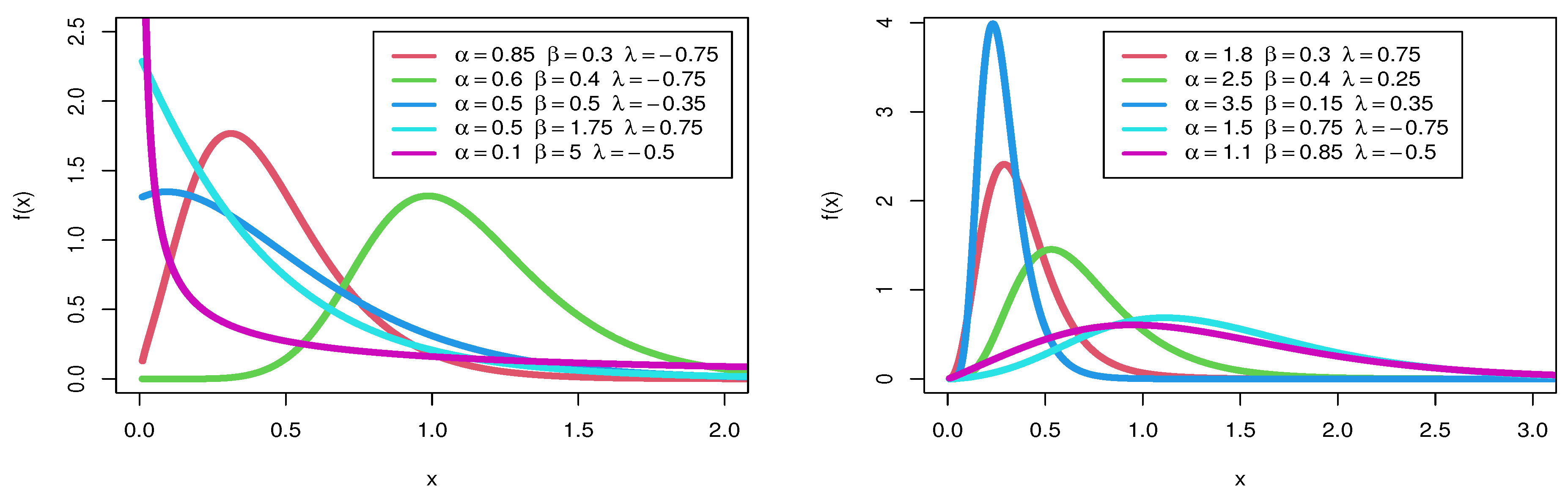
Depending on the values of its parameters,
Figure 1 shows some conceivable shapes of the
pdf. The
pdf can be take the following forms of a symmetrical, unimodal, asymmetrical, decreasing, right skewness and left skewness shape.
The survival function (sf) and the hazard or failure rate function (hrf) can indeed be expressed as
and
where,
The
model’s hazard rate plots are shown in
Figure 2. The hrf can be take the following forms: J shape, unimodal, a constant shape, and decreasing and increasing shape.
If
positive real non-integer and
then the binomial series expansion given by
If
. Then, the pdf of Equation (
6) can be represented linearly in a convenient way by
where
3. Mathematical Properties
Here, some fundamental mathematical aspects of distribution such as, , , , and for are discussed.
3.1. Ordinary Moments and Moment Generating Functions
are crucial in any statistical analysis and are valuable for quantifying skewness and kurtosis as well as for illuminating the distribution’s shape. If
X has pdf (
9) then the
of
X is given by
Setting
and after some algebra,
can indeed be expressed as
There are relationships between the behavior of a distribution’s
and distribution features such as the occurrence of moments. The
of
X may be obtained as follows from (
9):
3.2. Conditional Moments
The
upper incomplete (UI)
of
distribution is provided via
where
is the “UI gamma function”. In the same way, the
lower incomplete (LI)
of
distribution is denoted by
where
is the “LI gamma function”.
3.3. Entropy
After taking into consideration observable macroscopic variables such as temperature, pressure, and volume, the Rényi
represents the level of uncertainty that remains regarding a system. For the density function
, the Rényi
is characterized with (
From (
6), we have
using (
8) and after a few computations, we acquire
Then,
4. Bayesian and Classical Estimation Methods
We discussed the Bayesian and classical methods for unknown parameters of distribution.
4.1. Classical Methods
We investigated six classical estimation methods for unknown parameters of distribution.
4.1.1. Likelihood Estimation
The most common statistical inference technique is known as the ML estimates (MLEs) method. Consider a
random sample (
) of size
n drawn from the
distribution, and let
. The log-likelihood of
with
is given by
where
Now computing the first partial derivatives of (
17), we have
and
The MLEs
of
are computed by setting Equations (
18)–(
20) to 0 and solving them jointly.
4.1.2. Maximum Product Spacing (MPS) Estimators
The MPS technique was obtained by [
22] as an alternative to the MLE technique. If the order statistics of a
n from
are denoted by
, the MPS function of
can be defined as follows:
such that
. According to [
22], the MPSEs of unknown parameters are computed through maximization of the next formula.
Then, the MPS of
distribution is
Because the partial derivatives of MPS with regard to unknown parameters cannot be computed directly in closed mathematical formulas, we derive the MPS estimators using numerical approaches such as Newton–Raphson algorithms. For more information about and examples of this method see [
23,
24,
25].
4.1.3. Least Square (LS) and Weighted Least Square (WLS) Estimation
The LS and WLS estimate methods were presented by [
26]. Let
denote the order statistics of a
of size n from
. The LS estimations (LSE), and the Weighted LSE (WLSE) of the unknown parameters
and denoted by
and
can be derived via
where
. We obtained the LSE of the unknown parameters
when the
. Using partial derivatives of WLSE with regard to unknown parameters which these cannot be computed directly in closed mathematical formal, we derive the WLSE estimators using numerical approaches such as iterative algorithms. For more examples see [
27].
4.1.4. Cramér-Von Mises Estimation
The CVN method of estimation was established by [
28,
29] to estimate the unknown parameters and indicated by
are computed by
minimizing of goodness-of-fit statistic. Assume
simplify the order statistics of a
of size n from
, then, the CVN estimators can be obtained as follows:
By using partial derivatives of CVN estimators with respect to unknown parameters
which these cannot be computed directly in closed mathematical formal, we derive the CVN estimators using numerical approaches such as iterative algorithms.
4.1.5. Anderson-Darling Estimation
AD estimate (ADE) is another sort of minimal distance estimator that is obtained by minimizing AD statistics. Ref. [
30] proposed right-tail AD estimation as a refinement to the AD statistics. The ADE of the unknown parameters, represented by
are produced by minimizing the next formula with
.
By using partial derivatives of ADE with respect to unknown parameters
which these cannot be computed directly in closed mathematical formal, we derive the ADE using numerical approaches such as iterative algorithms.
4.2. Bayesian Estimation
In a Bayesian framework, unknown parameters in any model are handled as random variables rather than fixed constants. This is a reasonable assumption because the parameters of any population cannot remain constant throughout the research. By assuming prior distributions of unknown parameters, variance in the parameters can be accounted for. The parameters
and
are assumed to follow independent gamma prior distributions of the following forms:
and
where
, and
are called hyper-parameters. While the parameter
, we employ a uniform prior as a non-informative prior that expresses only a little bit of information about the parameters. To define prior distribution of
as uniform prior with interval −1 to 1. The density of uniform distribution is
. If
, and
then the prior distribution of
is
. The joint prior distribution of
is provided via
The joint posteriors distribution of
is obtained as follows:
The means of their respective marginal posteriors are Bayesian estimates (BEs) of the parameters under the squared error loss. As a result, the Bayesian estimators for
are:
By using Markov chain Monte Carlo (MCMC) techniques to derive Bayes estimates for the parameters because the above formulas are difficult to calculate analytically. For information about MCMC see [
31,
32]. The R programming language software is used to obtain the numerical results for the six methods of estimation.
5. Numerical Outcomes
The performance of the classical estimation methods and Bayesian method of the parameters
of the
distribution in terms of relative bias (
), and mean square errors (
) are evaluated in this section. We take into account the values 30, 80, and 150 for a sample size of
n. We generate random sample of
distribution by using numerical analysis, where we used “uniroot” function in R package after equating the CDF with the uniform distribution with n sample size and range 0 to 1. The following possibilities are taken into account for the parameters
: Case I:
, Case II:
, Case III:
, Case IV:
, Case V:
and Case VI:
. The
has been change from −0.5 to 0.7. we take replicating the process 5000 iterations. the
of the 160 estimations of the related
are obtained in each configuration. These numerical outcomes are displayed in
Table 1,
Table 2,
Table 3,
Table 4,
Table 5 and
Table 6. In
Table 1,
Table 2,
Table 3,
Table 4,
Table 5 and
Table 6, we conclude these points:
In each case, the MSEs fall as the n rises.
Additionally, the of estimates goes to zero values as sample size increases.
These results indicate that the classical estimation methods as ML, LS, WLS, CVN, and AD estimation approaches of the parameters , are asymptotically unbiased and consistent.
As anticipated, performance metrics show that estimates made using the Bayesian estimating approach outperform those made using the conventional estimation methods.
Bayesian estimators obtained under the assumption of the gamma priors are obtained for has non-informative priors.
6. Application of Real Data
This section uses two actual data sets to examine the adaptability and potential of the distribution. We offer a distribution application.
For the comparison of the models, We used different measures as the values of the Akaike information criterion (VAIC), Hannan Quinn information criterion (VHQIC), statistics of the Kolmogorov–Smirnov test (SKS), the statistics Anderson-Darling test (SAD), and the statistics Cramer-von Mises test (SCVM). Thus, the
distribution is compared with the transmuted Topp-Leone exponential (
) [
10], Marshall-Olkin LBE (MOLBE) [
33], the extention generalization of LBE (EGLBE) [
34], Marshal-Olkin Kumaraswamy moment exponential (MOKwME) [
35], and Gompertz Lomax (GL) [
36] distributions.
6.1. Precipitation Data
The March precipitation data set is given by [
37] which consists of 30 observations of the March precipitation (in inches) in Minneapolis/St Paul. The data are as follows: ‘0.77, 1.74, 0.81, 2.10, 0.52, 1.62, 1.31, 0.32, 0.59, 0.81, 2.81, 1.87, 1.20, 1.95, 1.20, 0.47, 1.43, 3.37, 2.20, 3.00, 3.09, 1.51, 1.18, 1.35, 4.75, 2.48, 0.96, 1.89, 0.90, 2.05’.
Figure 3 shows the estimated cdf with empirical cdf, probability of estimated pdf with histogram of data, and PP-plot for first data. In
Table 7, the
model has the largest
p-value and the lowest SKS for first data.
6.2. Times of Receiving an Analgesic
Data set II: 1.1, 1.4, 1.3, 1.7, 1.9, 1.8, 1.6, 2.2, 1.7, 2.7, 4.1, 1.8, 1.5, 1.2, 1.4, 3.0, 1.7, 2.3, 1.6, 2.0. these data discussed times of twenty patients receiving an analgesic which has used [
38] to fit the inverse power Lindley distribution. The fit of the empirical CDF, histogram, and PP-plot for data II were obtained in
Figure 4. The Bayesian estimates for the both data are provided in
Table 8. More ever the has the highest
p-value and the lowest SKS for
model have shown in
Table 9.
7. Competing Risks
Competing risks are frequent in time-to-event data, and regression analysis of such data has lately seen important methodological breakthroughs. In recent years, models were developed to estimate the lifespan of certain risks in the presence of other risk variables. The data for these "competing risk models" are the failure period and an indicator variable indicating the particular reason for the failure of the individual or item. It is possible to presume that the causes of failure are either independent or dependent. In most cases, the analysis of competing risk data presupposes that failures have separate causes. Despite the fact that the assumption of dependence is more realistic, there is some concern regarding the underlying model’s identifiability. Therefore, we introduced an alternative model based on competing risks. In this section, we consider the first type of data when there are causes of failure for the distribution.
The likelihood function of the
based on competing risk model is
where
, and
denoted two causes of failure, and
N is a sample size of two causes of failure, with
indicating that the cause of failure of
item is due to the first cause,
indicating that the cause of failure of
item is due to the second cause, and
indicating that the cause of failure of
unit is unknown, indicating that we do not know the real cause of failure for a test.
Using the first partial derivatives of log-likelihood of
based on competing risk model with respect to
, and
.To calculate the MLE
, and
from the nonlinear Equation (
32),we use the Newton–Raphson iterative method by substituting first partial derivatives of log-likelihood.
Furthermore, we compute the failure probability distribution of each failure cause in the presence of all others and the risk due to a particular failure cause.
The risk
due to cause
j:
where
j = 1 and 2.
When the integrated function in Equation (
33) is evaluated at the highest likelihood estimates of the parameters, the maximum likelihood estimate of
can be determined via numerical integration using the invariant condition. In order to create random draws from the posterior distribution of j for Bayesian analysis, we will combine the random draw from the joint distribution with the integral above, which we will then use to any Bayesian analysis we want on
;
1 and 2.
8. Analysis of Electrical Appliances with Two Causes of Failure
In this section, a real-life data set is explored (Lawless, [
39], p. 441). An automatic life test was performed on the 36 small electronic components. There are 18 main categories of failure. However, we discovered that only 7 of the 33 failure modes were represented and that only modes 6–9 occurred more than twice. Failure mode 9 is highly regarded. As a result, the data set contains two failure modes: = 1 (failure mode 9) and = 2 (all other failure modes) (failure time is censored). As a result, the following data shows the failure times in order, as well as the cause of each failure, if accessible. The following displays the data set: In first causes: 1167, 1925, 1990, 2223, 2400, 2471, 2551, 2568, 2694, 3034, 3112, 3214, 3478, 3504, 4329, 6976, 7846.
In second causes: 11, 35, 49, 170, 329, 381, 708, 958, 1062, 1594, 2327, 2451, 2702, 2761, 2831, 3059.
In cause of failure is unknown: 2565, 13403, 6367.
Table 10 show MLE with SE for each causes failure and SKS test with
p-value. Therefore, we note that this model is good fit of this data where
p-value is more than 0.05.
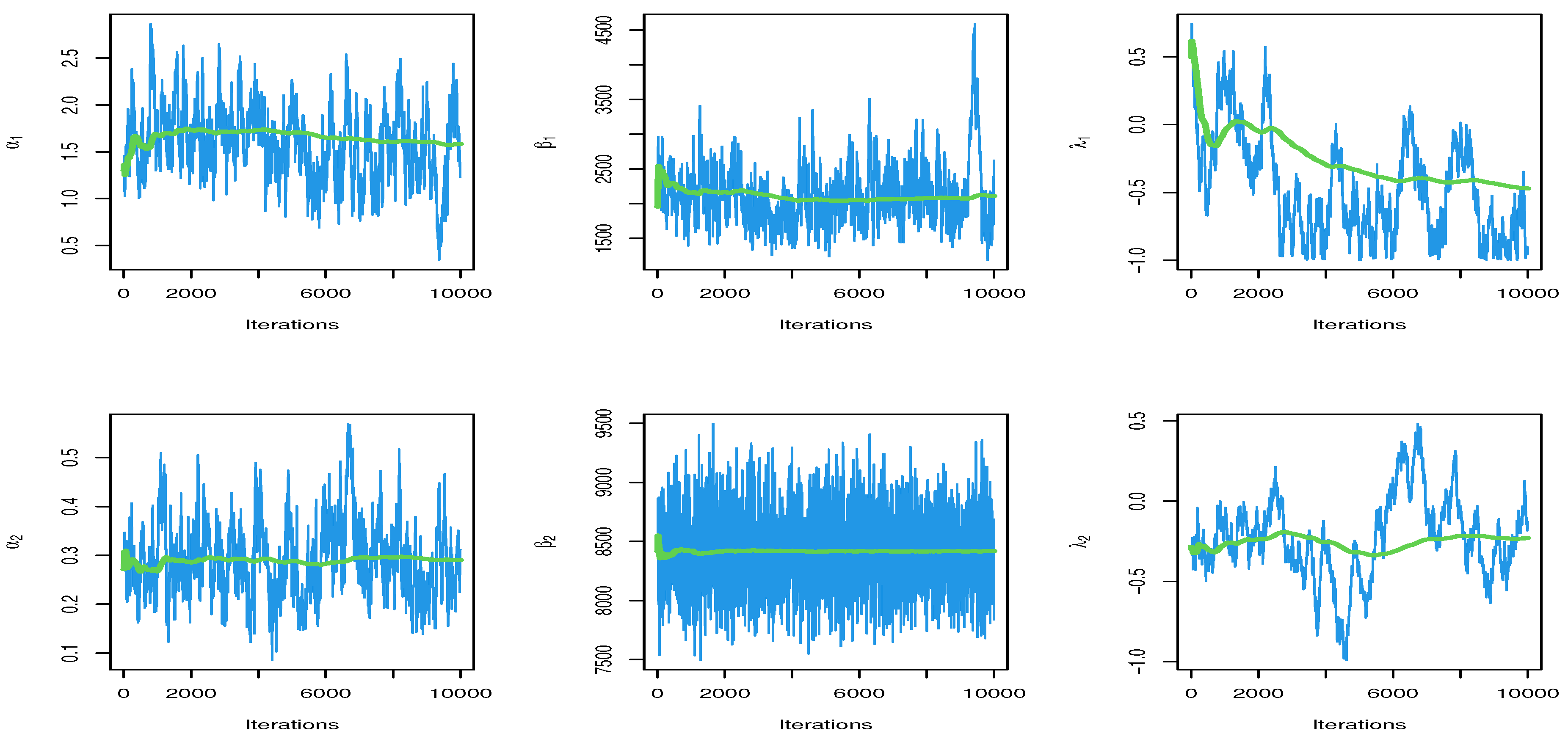
In order to examine the data,
Table 11 shows the MLE and BEs of the competing risk of
model with six parameters.
Figure 5 and
Figure 6 show the trace plots and marginal posterior density functions of parameters of the
distribution under competing risks produced using the Bayesian estimation approach, respectively.
Table 12 displays the relative risks calculated for each estimation technique. The trace and convergence plots of relative risks are shown in
Figure 7.
Figure 8 shows that the posterior density of MCMC results for each relative risk has a symmetric normal distribution.
9. Conclusions
We established competing risks models with k = 2 as independent causes of failure data in this paper. When the risks follow distributions, we computed the model’s likelihood equation and used it to derive the likelihood function. We wrote about how to achieve maximum likelihood and BEs for model parameters. For all unknown parameters with elective hyper parameters, we employed the gamma prior distribution in Bayesian analysis, and the parameter has uniform distribution with interval −1 to 1, and we used MCMC to generate random draws from the joint posterior distribution function. Farther more, we obtained different estimation method as six estimations for classical estimation methods and Bayesian estimation for parameter of . We conclude that Bayesian estimation is better than classical estimation methods. Using data analysis, we conclude that the distribution is more efficient than other models, such as TTLE, MOLBE, EGLBE, MOKwME, and GL distributions. While in analysis of electrical appliances with two causes of failure, the cause of failure is probably due to the first cause as shown in the previous results.
Author Contributions
Conceptualization, R.A.H.M., I.E. and H.M.A.; methodology, R.A.H.M., I.E., E.M.A., M.E. and H.M.A.; software, E.M.A. and M.E.; validation, R.A.H.M., I.E., E.M.A., M.E. and H.M.A.; formal analysis, R.A.H.M., I.E. and H.M.A.; investigation, R.A.H.M., M.E., I.E. and H.M.A.; resources, M.E., I.E. and E.M.A.; data curation, R.A.H.M., I.E., E.M.A., M.E. and H.M.A.; writing—original draft preparation, R.A.H.M., I.E., E.M.A., M.E. and H.M.A.; writing—review and editing, E.M.A. and M.E.; visualization, R.A.H.M. and H.M.A. All authors have read and agreed to the published version of the manuscript.
Funding
This research received no external funding.
Data Availability Statement
Data sets are available in this paper.
Conflicts of Interest
The authors declare no conflict of interest.
References
- Cordeiro, G.M.; de Castro, M. A new family of generalized distributions. J. Stat. Comput. Simul. 2011, 81, 883–898. [Google Scholar] [CrossRef]
- Algarni, A.; Almarashi, A.M.; Elbatal, I.; S. Hassan, A.; Almetwally, E.M.; MDaghistani, A.; Elgarhy, M. Type I half logistic Burr XG family: Properties, bayesian, and non-bayesian estimation under censored samples and applications to COVID-19 data. Math. Probl. Eng. 2021, 2021, 5461130. [Google Scholar] [CrossRef]
- Al-Shomrani, A.; Arif, O.; Shawky, A.; Hanif, S.; Shahbaz, M.Q. Topp–Leone family of distributions: Some properties and application. Pak. J. Stat. Oper. Res. 2016, 12, 443–451. [Google Scholar] [CrossRef] [Green Version]
- Elbatal, I.; Alotaibi, N.; Almetwally, E.M.; Alyami, S.A.; Elgarhy, M. On Odd Perks-G Class of Distributions: Properties, Regression Model, Discretization, Bayesian and Non-Bayesian Estimation, and Applications. Symmetry 2022, 14, 883. [Google Scholar] [CrossRef]
- Bourguignon, M.; Silva, R.B.; Cordeiro, G.M. The Weibull-G family of probability distributions. J. Data Sci. 2014, 12, 53–68. [Google Scholar] [CrossRef]
- Al-Babtain, A.A.; Elbatal, I.; Chesneau, C.; Elgarhy, M. Sine Topp-Leone-G family of distributions: Theory and applications. Open Phys. 2020, 18, 74–593. [Google Scholar] [CrossRef]
- Bantan, R.A.; Jamal, F.; Chesneau, C.; Elgarhy, M. Type II Power Topp–Leone Generated Family of Distributions with Applications. Symmetry 2020, 12, 75. [Google Scholar] [CrossRef] [Green Version]
- Almetwally, E.M.; Kilai, M.; Aldallal, R. X-Gamma Lomax Distribution with Different Applications. J. Bus. Environ. Sci. 2022, 1, 129–140. [Google Scholar] [CrossRef]
- Bantan, R.A.; Jamal, F.; Chesneau, C.; Elgarhy, M. A New Power Topp–Leone Generated Family of Distributions with Applications. Entropy 2019, 21, 1177. [Google Scholar] [CrossRef] [Green Version]
- Yousof, H.M.; Alizadeh, M.; Jahanshahi, S.M.; Ghosh, T.G.; Hamedani, G.G. The transmuted Topp-Leone G family of distributions: Theory, characterizations and applications. J. Data Sci. 2017, 15, 723–740. [Google Scholar] [CrossRef]
- Shaw, W.T.; Buckley, I.R. The alchemy of probability distributions: Beyond Gram–Charlier expansions, and a skew-kurtotic-normal distribution from a rank transmutation map. arXiv 2009, arXiv:0901.0434. [Google Scholar]
- Dara, S.; Ahmad, M. Recent Advances in Moments Distributions and Their Hazard Rate. Ph.D. Thesis, National College of Business Administration and Economics, Lahore, Pakistan, 2012. [Google Scholar]
- Khaleel, M.A.; Ibrahim, N.A.; Shitan, M.; Merovci, F. New extension of Burr type X distribution properties with application. J. King Saud Univ.-Sci. 2018, 30, 450–457. [Google Scholar] [CrossRef]
- Chakraborty, S.; Handique, L.; Usman, R.M. A simple extension of Burr-III distribution and its advantages over existing ones in modelling failure time data. Ann. Data Sci. 2020, 7, 17–31. [Google Scholar] [CrossRef]
- Kamal, R.M.; Ismail, M.A. The Flexible Weibull Extension-Burr XII Distribution: Model, Properties and Applications. Pak. J. Stat. Oper. Res. 2020, 16, 447–460. [Google Scholar] [CrossRef]
- Nasir, M.A.; Tahir, M.H.; Jamal, F.; Ozel, G. A new generalized Burr family of distributions for the lifetime data. J. Stat. Appl. Probab. 2017, 6, 401–417. [Google Scholar] [CrossRef]
- Sarhan, A.M.; Hamilton, D.C.; Smith, B. Statistical analysis of competing risks models. Reliab. Eng. Syst. Saf. 2010, 95, 953–962. [Google Scholar] [CrossRef]
- Bakoban, R.A.; Abd-Elmougod, G.A. MCMC in analysis of progressively first failure censored competing risks data for gompertz model. J. Comput. Theor. Nanosci. 2016, 13, 6662–6670. [Google Scholar] [CrossRef]
- Liu, F.; Shi, Y. Inference for a simple step-stress model with progressively censored competing risks data from Weibull distribution. Commun. Stat.-Theory Methods 2017, 46, 7238–7255. [Google Scholar] [CrossRef]
- Abushal, T.A.; Soliman, A.A.; Abd-Elmougod, G.A. Inference of partially observed causes for failure of Lomax competing risks model under type-II generalized hybrid censoring scheme. Alex. Eng. J. 2022, 61, 5427–5439. [Google Scholar] [CrossRef]
- Wang, L.; Tripathi, Y.M.; Dey, S.; Shi, Y. Inference for dependence competing risks with partially observed failure causes from bivariate Gompertz distribution under generalized progressive hybrid censoring. Qual. Reliab. Eng. Int. 2021, 37, 1150–1172. [Google Scholar] [CrossRef]
- Cheng, R.C.; Amin, N.A. Estimating parameters in continuous univariate distributions with a shifted origin. J. R. Stat. Soc. Ser. B (Methodol.) 1983, 45, 394–403. [Google Scholar] [CrossRef]
- Sabry, M.A.; Almetwally, E.M.; Almongy, H.M. Monte Carlo Simulation of Stress-Strength Model and Reliability Estimation for Extension of the Exponential Distribution. Thail. Stat. 2022, 20, 124–143. [Google Scholar]
- Sabry, M.A.; Almetwally, E.M.; Alamri, O.A.; Yusuf, M.; Almongy, H.M.; Eldeeb, A.S. Inference of fuzzy reliability model for inverse Rayleigh distribution. AIMS Math. 2021, 6, 9770–9785. [Google Scholar] [CrossRef]
- Almongy, H.M.; Alshenawy, F.Y.; Almetwally, E.M.; Abdo, D.A. Applying transformer insulation using Weibull extended distribution based on progressive censoring scheme. Axioms 2021, 10, 100. [Google Scholar] [CrossRef]
- Swain, J.J.; Venkatraman, S.; Wilson, J.R. Least-squares estimation of distribution functions in Johnson’s translation system. J. Stat. Comput. Simul. 1988, 29, 271–297. [Google Scholar] [CrossRef]
- Almongy, H.M.; Almetwally, E.M. Robust estimation methods of generalized exponential distribution with outliers. Pak. J. Stat. Oper. Res. 2020, 16, 545–559. [Google Scholar] [CrossRef]
- Mises, R.V. Wahrscheinlichkeit Statistik und Wahrheit; Springer: Berlin/Heidelberg, Germany, 2013. [Google Scholar]
- Cramér, H. On the Composition of Elementary Errors: Statistical Applications; Almqvist and Wiksell: Stockholm, Sweden, 1928. [Google Scholar]
- Luceño, A. Fitting the generalized Pareto distribution to data using maximum goodness-of-fit estimators. Comput. Stat. Data Anal. 2006, 51, 904–917. [Google Scholar] [CrossRef]
- Gelf, A.E.; Smith, A.F. Sampling-based approaches to calculating marginal densities. J. Am. Stat. Assoc. 1990, 85, 398–409. [Google Scholar]
- Hastings, W.K. Monte Carlo sampling methods using Markov chains and their applications. Biometrika 1970, 57, 97–109. [Google Scholar] [CrossRef]
- ul Haq, M.A.; Usman, R.M.; Hashmi, S.; Al-Omeri, A.I. The Marshall-Olkin length-biased exponential distribution and its applications. J. King Saud-Univ.-Sci. 2019, 31, 246–251. [Google Scholar] [CrossRef]
- Maxwell, O.; Oyamakin, S.O.; Chukwu, A.U.; Olusola, Y.O.; Kayode, A.A. New generalization of length biased exponential distribution with applications. J. Adv. Appl. Math. 2019, 4, 82–88. [Google Scholar] [CrossRef]
- Ahmadini, A.A.; Hassan, A.S.; Mohamed, R.E.; Alshqaq, S.S.; Nagy, H.F. A New four-parameter moment exponential model with applications to lifetime data. Intell. Autom. Soft Comput. 2021, 29, 131–146. [Google Scholar] [CrossRef]
- Oguntunde, P.E.; Khaleel, M.A.; Ahmed, M.T.; Adejumo, A.O.; Odetunmibi, O.A. A new generalization of the Lomax distribution with increasing, decreasing, and constant failure rate. Model. Simul. Eng. 2017, 2017, 6043169. [Google Scholar] [CrossRef]
- Reyad, H.; Jamal, F.; Othman, S.; Yahia, N. The Topp Leone generalized inverted Kumaraswamy distribution: Properties and applications. Asian Res. J. Math. 2019, 13, 1–15. [Google Scholar] [CrossRef]
- Barco, K.V.; Mazucheli, J.; Janeiro, V. The inverse power Lindley distribution. Commun. Stat.-Simul. Comput. 2017, 46, 6308–6323. [Google Scholar] [CrossRef]
- Lawless, J.F. Statistical Models and Methods for Lifetime Data; John Wiley & Sons: Hoboken, NJ, USA, 2011; p. 362. [Google Scholar]
Figure 1.
pdf of distribution.
Figure 1.
pdf of distribution.
Figure 2.
hrf of distribution.
Figure 2.
hrf of distribution.
Figure 3.
Estimated CDF, empirical CDF, estimated PDF with histogram, and P-P plot for the TTLLE distribution for data set 1.
Figure 3.
Estimated CDF, empirical CDF, estimated PDF with histogram, and P-P plot for the TTLLE distribution for data set 1.
Figure 4.
Estimated CDF, empirical CDF, estimated PDF with histogram, and P-P plot for the TTLLE distribution for data set 2.
Figure 4.
Estimated CDF, empirical CDF, estimated PDF with histogram, and P-P plot for the TTLLE distribution for data set 2.
Figure 5.
Trace for parameters of MCMC results.
Figure 5.
Trace for parameters of MCMC results.
Figure 6.
The posterior density for parameters of MCMC results.
Figure 6.
The posterior density for parameters of MCMC results.
Figure 7.
Trace for relative risks of MCMC results.
Figure 7.
Trace for relative risks of MCMC results.
Figure 8.
The posterior density for relative risks of MCMC results.
Figure 8.
The posterior density for relative risks of MCMC results.
Table 1.
Numerical outcomes of and for all estimation approaches at Case I.
Table 1.
Numerical outcomes of and for all estimation approaches at Case I.
| MLE | LS | WLS | MPS | CVM | AD | Bayesian |
|---|
| n | | | | | | | | | | | | | | | |
|---|
| −0.5 | 30 | | −0.1149 | 0.3790 | −0.0066 | 0.4685 | −0.0058 | 0.3858 | −0.1152 | 0.2472 | 0.1042 | 0.7527 | 0.0063 | 0.3256 | −0.0112 | 0.0282 |
| 0.1705 | 0.0844 | 0.1153 | 0.1583 | 0.1029 | 0.1406 | 0.1718 | 0.2000 | 0.0502 | 0.1119 | 0.0796 | 0.1139 | 0.0058 | 0.0155 |
| −0.2568 | 0.2541 | −0.1937 | 0.4160 | −0.1845 | 0.3676 | −0.2607 | 0.4914 | −0.0889 | 0.3883 | −0.1455 | 0.3752 | 0.0087 | 0.0267 |
| 80 | | −0.0746 | 0.1628 | 0.0192 | 0.1288 | 0.0141 | 0.1198 | −0.0748 | 0.1372 | 0.0666 | 0.1616 | 0.0216 | 0.1120 | 0.0012 | 0.0141 |
| 0.1095 | 0.0420 | 0.0692 | 0.0611 | 0.0587 | 0.0514 | 0.1095 | 0.0838 | 0.0449 | 0.0499 | 0.0545 | 0.0509 | 0.0003 | 0.0068 |
| −0.2787 | 0.2286 | −0.3059 | 0.2402 | −0.2630 | 0.2273 | −0.2776 | 0.2953 | −0.2859 | 0.2329 | −0.2665 | 0.2299 | 0.0007 | 0.0152 |
| 150 | | −0.0593 | 0.1237 | 0.0109 | 0.0868 | 0.0267 | 0.0915 | −0.0590 | 0.1142 | 0.0417 | 0.0953 | 0.0318 | 0.0912 | 0.0003 | 0.0069 |
| 0.0774 | 0.0304 | 0.0483 | 0.0342 | 0.0434 | 0.0300 | 0.0775 | 0.0525 | 0.0359 | 0.0300 | 0.0435 | 0.0300 | −0.0020 | 0.0033 |
| −0.1799 | 0.1966 | −0.2166 | 0.1896 | −0.2533 | 0.1846 | −0.1814 | 0.2334 | −0.2281 | 0.1849 | −0.2700 | 0.1931 | 0.0020 | 0.0063 |
| 0.7 | 30 | | −0.1695 | 0.1487 | −0.0319 | 0.2496 | −0.0273 | 0.1800 | −0.1670 | 0.1550 | 0.0629 | 0.3629 | −0.0180 | 0.1422 | −0.0157 | 0.0212 |
| 0.2735 | 0.0898 | 0.1343 | 0.4206 | 0.0995 | 0.2444 | 0.2681 | 0.3423 | 0.1153 | 0.4064 | 0.1103 | 0.2273 | 0.0030 | 0.0256 |
| 0.2485 | 0.1299 | 0.0138 | 0.2845 | 0.0081 | 0.2138 | 0.2428 | 0.2052 | 0.1424 | 0.2630 | 0.1247 | 0.2003 | 0.0265 | 0.0315 |
| 80 | | −0.0821 | 0.0781 | −0.0214 | 0.1101 | −0.0128 | 0.0899 | −0.0818 | 0.0744 | 0.0117 | 0.1222 | −0.0062 | 0.0840 | 0.0005 | 0.0204 |
| 0.1125 | 0.0593 | 0.0643 | 0.1685 | 0.0460 | 0.1202 | 0.1122 | 0.1296 | 0.0425 | 0.1548 | 0.0399 | 0.1091 | −0.0017 | 0.0101 |
| 0.0728 | 0.1146 | 0.0194 | 0.1335 | −0.0020 | 0.0982 | 0.0721 | 0.0755 | 0.0205 | 0.1453 | 0.0067 | 0.0937 | −0.0079 | 0.0142 |
| 150 | | −0.0514 | 0.0408 | −0.0103 | 0.0623 | −0.0017 | 0.0511 | −0.0516 | 0.0403 | 0.0080 | 0.0668 | 0.0007 | 0.0460 | −0.0050 | 0.0070 |
| 0.0732 | 0.0483 | 0.0372 | 0.0969 | 0.0253 | 0.0720 | 0.0732 | 0.0781 | 0.0222 | 0.0948 | 0.0200 | 0.0612 | 0.0041 | 0.0046 |
| 0.0335 | 0.0955 | −0.0219 | 0.0943 | −0.0291 | 0.0695 | 0.0339 | 0.0557 | −0.0371 | 0.1074 | −0.0295 | 0.0662 | −0.0033 | 0.0075 |
Table 2.
Numerical outcomes of and for all estimation approaches at Case II.
Table 2.
Numerical outcomes of and for all estimation approaches at Case II.
| MLE | LS | WLS | MPS | CVM | AD | Bayesian |
|---|
| n | | | | | | | | | | | | | | | |
|---|
| −0.5 | 30 | | −0.0376 | 0.0532 | 0.0130 | 0.0375 | 0.0225 | 0.0273 | −0.0395 | 0.0271 | 0.1405 | 0.0483 | 0.0801 | 0.0316 | 0.0471 | 0.0102 |
| 0.2052 | 0.0896 | 0.1371 | 0.2078 | 0.1340 | 0.1862 | 0.2020 | 0.2352 | 0.0643 | 0.1542 | 0.1102 | 0.1787 | −0.0056 | 0.0205 |
| −0.3249 | 0.2273 | −0.0751 | 0.2548 | −0.2132 | 0.2627 | −0.3114 | 0.3207 | −0.2017 | 0.2416 | −0.2922 | 0.3006 | −0.0228 | 0.0266 |
| 80 | | −0.0359 | 0.0219 | 0.0873 | 0.0167 | 0.0627 | 0.0162 | −0.0377 | 0.0183 | 0.0967 | 0.0195 | 0.0602 | 0.0162 | −0.0030 | 0.0040 |
| 0.1227 | 0.0443 | 0.0822 | 0.0797 | 0.0695 | 0.0740 | 0.1215 | 0.1413 | 0.0470 | 0.0635 | 0.0516 | 0.0593 | 0.0054 | 0.0120 |
| −0.2553 | 0.2045 | −0.4739 | 0.2656 | −0.3782 | 0.2576 | −0.2480 | 0.2842 | −0.3619 | 0.2419 | −0.3168 | 0.2226 | −0.0360 | 0.0170 |
| 150 | | −0.0176 | 0.0162 | 0.0662 | 0.0122 | 0.0833 | 0.0122 | −0.0178 | 0.0135 | 0.0964 | 0.0138 | 0.0708 | 0.0119 | 0.0064 | 0.0025 |
| 0.0826 | 0.0407 | 0.0530 | 0.0490 | 0.0510 | 0.0524 | 0.0831 | 0.0788 | 0.0398 | 0.0443 | 0.0381 | 0.0404 | 0.0032 | 0.0048 |
| −0.1894 | 0.1937 | −0.3135 | 0.1715 | −0.3759 | 0.1892 | −0.1893 | 0.2154 | −0.3497 | 0.1741 | −0.2982 | 0.1601 | −0.0128 | 0.0072 |
| 0.7 | 30 | | −0.1050 | 0.0105 | 0.0747 | 0.0210 | 0.0481 | 0.0150 | −0.1048 | 0.0088 | 0.1432 | 0.0268 | 0.0410 | 0.0107 | 0.0197 | 0.0044 |
| 0.4285 | 0.0857 | 0.0103 | 0.2200 | 0.1281 | 0.4462 | 0.4174 | 2.4423 | −0.0116 | 0.3800 | 0.1881 | 0.8247 | 0.0417 | 0.0423 |
| 0.1472 | 0.1940 | −0.0210 | 0.1157 | 0.1200 | 0.1035 | 0.1561 | 0.2939 | 0.0361 | 0.1034 | 0.2174 | 0.1449 | −0.0132 | 0.0231 |
| 80 | | −0.0957 | 0.0053 | −0.0291 | 0.0060 | −0.0252 | 0.0042 | −0.0934 | 0.0064 | −0.0050 | 0.0062 | −0.0186 | 0.0043 | −0.0044 | 0.0012 |
| 0.1113 | 0.0857 | 0.0402 | 0.2335 | 0.0555 | 0.1663 | 0.1194 | 0.1246 | −0.0172 | 0.1750 | 0.0423 | 0.1236 | 0.0162 | 0.0170 |
| −0.0407 | 0.1825 | −0.0515 | 0.1156 | 0.0085 | 0.0691 | −0.0217 | 0.1429 | −0.0902 | 0.1294 | 0.0165 | 0.0706 | 0.0070 | 0.0130 |
| 150 | | −0.0533 | 0.0033 | −0.0234 | 0.0036 | −0.0163 | 0.0032 | −0.0461 | 0.0035 | −0.0109 | 0.0036 | −0.0145 | 0.0030 | 0.0112 | 0.0010 |
| 0.1032 | 0.0809 | 0.1176 | 0.2587 | 0.0888 | 0.1279 | 0.1268 | 0.1293 | 0.0998 | 0.2545 | 0.0826 | 0.1110 | 0.0005 | 0.0053 |
| 0.0496 | 0.1033 | 0.0852 | 0.0904 | 0.0699 | 0.0582 | 0.0584 | 0.0526 | 0.0832 | 0.0965 | 0.0705 | 0.0554 | 0.0177 | 0.0059 |
Table 3.
Numerical outcomes of and for all estimation approaches at Case III.
Table 3.
Numerical outcomes of and for all estimation approaches at Case III.
| MLE | LS | WLS | MPS | CVM | AD | Bayesian |
|---|
| n | | | | | | | | | | | | | | | |
|---|
| −0.5 | 30 | | −0.0623 | 0.0649 | −0.1031 | 0.0486 | −0.0700 | 0.0364 | −0.0820 | 0.0630 | −0.0035 | 0.0553 | 0.0149 | 0.0599 | 0.0330 | 0.0255 |
| 0.3173 | 0.0304 | 0.2288 | 0.0678 | 0.2235 | 0.0666 | 0.3150 | 0.1103 | 0.1279 | 0.0324 | 0.1848 | 0.0516 | 0.0293 | 0.0051 |
| −0.8728 | 0.3038 | −0.4305 | 0.2958 | −0.5657 | 0.3615 | −0.8058 | 0.4666 | −0.3767 | 0.2332 | −0.6773 | 0.3645 | −0.0329 | 0.0179 |
| 80 | | −0.0719 | 0.0553 | 0.0524 | 0.0518 | 0.0647 | 0.0441 | −0.0750 | 0.0491 | 0.1060 | 0.0619 | 0.0992 | 0.0451 | 0.0096 | 0.0127 |
| 0.0821 | 0.0117 | 0.0689 | 0.0171 | 0.0665 | 0.0157 | 0.0836 | 0.0141 | 0.0431 | 0.0143 | 0.0698 | 0.0158 | 0.0084 | 0.0022 |
| −0.0368 | 0.2382 | −0.3075 | 0.2501 | −0.3732 | 0.2532 | −0.0290 | 0.1713 | −0.3343 | 0.2451 | −0.4874 | 0.2882 | −0.0057 | 0.0172 |
| 150 | | −0.1239 | 0.0433 | 0.0321 | 0.0328 | 0.0039 | 0.0372 | −0.1122 | 0.0352 | 0.0533 | 0.0356 | 0.0214 | 0.0345 | 0.0050 | 0.0028 |
| 0.0728 | 0.0038 | 0.0985 | 0.0141 | 0.0714 | 0.0093 | 0.0737 | 0.0064 | 0.0842 | 0.0122 | 0.0643 | 0.0079 | 0.0040 | 0.0009 |
| 0.1236 | 0.1213 | −0.4028 | 0.2751 | −0.2164 | 0.1948 | 0.0930 | 0.1242 | −0.3992 | 0.2715 | −0.2475 | 0.1826 | 0.0009 | 0.0067 |
| 0.7 | 30 | | −0.0727 | 0.0341 | 0.0161 | 0.0306 | 0.0185 | 0.0245 | −0.0777 | 0.0230 | 0.1039 | 0.0482 | 0.0549 | 0.0277 | −0.0178 | 0.0088 |
| 0.3313 | 0.0253 | 0.0573 | 0.0775 | 0.0653 | 0.0814 | 0.3140 | 0.2912 | −0.0164 | 0.0588 | 0.0303 | 0.0726 | 0.0285 | 0.0078 |
| 0.2254 | 0.0976 | 0.0415 | 0.1905 | 0.0613 | 0.1773 | 0.2184 | 0.3101 | 0.0382 | 0.1867 | 0.0498 | 0.1844 | 0.0673 | 0.0310 |
| 80 | | −0.0766 | 0.0153 | −0.0370 | 0.0148 | −0.0404 | 0.0108 | −0.0849 | 0.0140 | −0.0079 | 0.0153 | −0.0354 | 0.0105 | 0.0113 | 0.0068 |
| 0.0649 | 0.0087 | −0.0104 | 0.0159 | 0.0103 | 0.0085 | 0.0763 | 0.0137 | −0.0347 | 0.0165 | 0.0066 | 0.0074 | −0.0218 | 0.0056 |
| 0.0058 | 0.0883 | −0.0962 | 0.0596 | −0.0256 | 0.0344 | −0.0030 | 0.0246 | −0.0953 | 0.0658 | −0.0175 | 0.0327 | 0.0018 | 0.0147 |
| 150 | | −0.0622 | 0.0097 | −0.0388 | 0.0142 | −0.0291 | 0.0122 | −0.0647 | 0.0117 | −0.0243 | 0.0140 | −0.0260 | 0.0112 | 0.0101 | 0.0032 |
| 0.0612 | 0.0076 | 0.1253 | 0.0457 | 0.0917 | 0.0254 | 0.1271 | 0.0214 | 0.1087 | 0.0455 | 0.0776 | 0.0224 | 0.0004 | 0.0024 |
| 0.1194 | 0.0705 | 0.1409 | 0.0982 | 0.1061 | 0.0622 | 0.1246 | 0.0382 | 0.1320 | 0.1079 | 0.0870 | 0.0609 | −0.0017 | 0.0064 |
Table 4.
Numerical outcomes of and for all estimation approaches at Case IV.
Table 4.
Numerical outcomes of and for all estimation approaches at Case IV.
| MLE | LS | WLS | MPS | CVM | AD | Bayesian |
|---|
| n | | | | | | | | | | | | | | | |
|---|
| −0.5 | 30 | | −0.1503 | 1.6970 | 0.0508 | 5.5365 | 0.0319 | 4.7037 | −0.1503 | 1.3470 | 0.2140 | 10.0191 | 0.0350 | 2.4918 | −0.0021 | 0.0333 |
| 0.1709 | 0.0606 | 0.1019 | 0.1342 | 0.0952 | 0.1269 | 0.1707 | 0.1752 | 0.0427 | 0.1061 | 0.0737 | 0.1018 | 0.0036 | 0.0116 |
| −0.2708 | 0.2184 | −0.1638 | 0.4286 | −0.1276 | 0.4589 | −0.2704 | 0.8417 | −0.0353 | 0.4252 | −0.1455 | 0.4311 | −0.0091 | 0.0281 |
| 80 | | −0.1181 | 0.5155 | −0.0149 | 0.6503 | −0.0125 | 0.5227 | −0.1183 | 0.5623 | 0.0373 | 0.7706 | −0.0001 | 0.5001 | 0.0005 | 0.0179 |
| 0.0983 | 0.0298 | 0.0698 | 0.0543 | 0.0572 | 0.0446 | 0.0983 | 0.0676 | 0.0484 | 0.0449 | 0.0516 | 0.0403 | 0.0056 | 0.0060 |
| −0.2006 | 0.1795 | −0.2627 | 0.2491 | −0.2212 | 0.2179 | −0.2000 | 0.2640 | −0.2415 | 0.2439 | −0.2255 | 0.2154 | 0.0047 | 0.0154 |
| 150 | | −0.0810 | 0.4055 | −0.0093 | 0.3587 | 0.0014 | 0.3279 | −0.0819 | 0.4438 | 0.0197 | 0.3935 | 0.0011 | 0.3124 | −0.0007 | 0.0076 |
| 0.0875 | 0.0279 | 0.0510 | 0.0299 | 0.0477 | 0.0281 | 0.0876 | 0.0552 | 0.0390 | 0.0262 | 0.0463 | 0.0276 | 0.0008 | 0.0042 |
| −0.1930 | 0.1621 | −0.2517 | 0.2090 | −0.2792 | 0.2042 | −0.2991 | 0.2911 | −0.2385 | 0.2014 | −0.2711 | 0.2060 | 0.0014 | 0.0078 |
| 0.7 | 30 | | −0.1095 | 2.7815 | 0.0195 | 2.3716 | 0.0259 | 2.1963 | −0.1094 | 1.5471 | 0.1496 | 3.5821 | 0.0585 | 2.1930 | 0.0012 | 0.0338 |
| 0.1787 | 0.0676 | 0.0923 | 0.5021 | 0.0837 | 0.4213 | 0.1782 | 0.5923 | 0.0553 | 0.4968 | 0.0703 | 0.3180 | 0.0031 | 0.0284 |
| 0.0771 | 0.1742 | −0.0310 | 0.4648 | −0.0220 | 0.3950 | 0.0770 | 0.5293 | 0.0504 | 0.5678 | 0.0346 | 0.3238 | −0.0212 | 0.0284 |
| 80 | | −0.0729 | 0.4430 | −0.0093 | 0.4628 | 0.0091 | 0.4188 | −0.0765 | 0.3342 | 0.0309 | 0.5217 | 0.0223 | 0.4024 | −0.0078 | 0.0240 |
| 0.0672 | 0.0449 | 0.0421 | 0.1158 | 0.0110 | 0.0601 | 0.0723 | 0.0581 | 0.0251 | 0.1132 | −0.0039 | 0.0337 | 0.0108 | 0.0072 |
| 0.0511 | 0.0729 | 0.0129 | 0.1565 | −0.0544 | 0.1269 | 0.0567 | 0.0462 | 0.0175 | 0.1694 | −0.0682 | 0.1120 | −0.0313 | 0.0196 |
| 150 | | −0.0439 | 0.3387 | 0.0245 | 0.4700 | 0.0236 | 0.3708 | −0.0438 | 0.2737 | 0.0479 | 0.5301 | 0.0260 | 0.3449 | −0.0012 | 0.0090 |
| 0.0451 | 0.0385 | 0.0022 | 0.0644 | 0.0023 | 0.0474 | 0.0450 | 0.0406 | −0.0052 | 0.0651 | 0.0013 | 0.0435 | 0.0031 | 0.0033 |
| 0.0093 | 0.0710 | −0.0984 | 0.1473 | −0.0717 | 0.1014 | 0.0088 | 0.0629 | −0.0882 | 0.1483 | −0.0615 | 0.0935 | 0.0010 | 0.0070 |
Table 5.
Numerical outcomes of and for all estimation approaches at Case V.
Table 5.
Numerical outcomes of and for all estimation approaches at Case V.
| MLE | LS | WLS | MPS | CVM | AD | Bayesian |
|---|
| n | | | | | | | | | | | | | | | |
|---|
| −0.5 | 30 | | −0.1621 | 1.6092 | 0.0298 | 3.8896 | 0.0169 | 3.3786 | −0.1625 | 1.4882 | 0.1862 | 6.9558 | 0.0258 | 2.3133 | −0.0041 | 0.0326 |
| 0.1665 | 0.2383 | 0.1015 | 0.5080 | 0.0920 | 0.4424 | 0.1667 | 0.6317 | 0.0427 | 0.3620 | 0.0712 | 0.3465 | −0.0009 | 0.0262 |
| −0.3106 | 0.2255 | −0.2487 | 0.3219 | −0.1774 | 0.3739 | −0.3101 | 0.4194 | −0.1424 | 0.3270 | −0.1816 | 0.3171 | −0.0053 | 0.0283 |
| 80 | | −0.1105 | 0.5318 | −0.0058 | 0.7491 | −0.0066 | 0.6145 | −0.1103 | 0.6595 | 0.0387 | 0.9040 | 0.0051 | 0.5715 | 0.0015 | 0.0169 |
| 0.1017 | 0.1313 | 0.0648 | 0.2070 | 0.0567 | 0.1843 | 0.1016 | 0.2920 | 0.0410 | 0.1655 | 0.0512 | 0.1625 | 0.0009 | 0.0116 |
| −0.2627 | 0.1939 | −0.2770 | 0.2339 | −0.2548 | 0.2279 | −0.2623 | 0.2915 | −0.2103 | 0.2184 | −0.2618 | 0.2237 | −0.0111 | 0.0149 |
| 150 | | −0.0887 | 0.3818 | 0.0083 | 0.4219 | 0.0038 | 0.3608 | −0.0887 | 0.4627 | 0.0364 | 0.4787 | 0.0080 | 0.3579 | −0.0010 | 0.0082 |
| 0.0749 | 0.1035 | 0.0512 | 0.1347 | 0.0447 | 0.1182 | 0.0748 | 0.1916 | 0.0393 | 0.1239 | 0.0457 | 0.1238 | 0.0013 | 0.0061 |
| −0.1971 | 0.1882 | −0.3025 | 0.2187 | −0.2652 | 0.2030 | −0.1964 | 0.2463 | −0.2816 | 0.2118 | −0.2858 | 0.2150 | −0.0009 | 0.0070 |
| 0.7 | 30 | | −0.1368 | 1.9840 | 0.0128 | 1.9481 | 0.0141 | 1.7599 | −0.1378 | 1.1393 | 0.1403 | 2.9613 | 0.0379 | 1.6846 | −0.0036 | 0.0312 |
| 0.2126 | 0.2651 | 0.0809 | 1.0598 | 0.0901 | 0.9971 | 0.2117 | 2.2453 | 0.0405 | 0.9890 | 0.0769 | 0.9227 | −0.0039 | 0.0326 |
| 0.2043 | 0.1724 | −0.0040 | 0.4591 | 0.0452 | 0.3101 | 0.1989 | 0.5817 | 0.0440 | 0.4282 | 0.0775 | 0.3202 | −0.0163 | 0.0283 |
| 80 | | −0.0885 | 0.5320 | −0.0165 | 0.7109 | −0.0068 | 0.5603 | −0.0879 | 0.4432 | 0.0259 | 0.8218 | 0.0072 | 0.5301 | 0.0000 | 0.0173 |
| 0.0886 | 0.1871 | 0.0563 | 0.4739 | 0.0455 | 0.3388 | 0.0882 | 0.3448 | 0.0415 | 0.4677 | 0.0256 | 0.2752 | −0.0018 | 0.0141 |
| 0.0526 | 0.1618 | 0.0133 | 0.1885 | 0.0246 | 0.1126 | 0.0530 | 0.0878 | 0.0292 | 0.1934 | −0.0203 | 0.1252 | −0.0211 | 0.0144 |
| 150 | | −0.0553 | 0.3157 | 0.0081 | 0.3938 | 0.0090 | 0.3190 | −0.0556 | 0.2560 | 0.0302 | 0.4406 | 0.0118 | 0.2990 | −0.0008 | 0.0075 |
| 0.0525 | 0.1540 | 0.0123 | 0.2701 | 0.0096 | 0.1922 | 0.0527 | 0.1634 | 0.0071 | 0.2753 | 0.0071 | 0.1732 | 0.0011 | 0.0063 |
| 0.0293 | 0.1092 | −0.0712 | 0.1356 | −0.0549 | 0.0954 | 0.0295 | 0.0513 | −0.0530 | 0.1328 | −0.0520 | 0.0904 | −0.0050 | 0.0066 |
Table 6.
Numerical outcomes of and for all estimation approaches at Case VI.
Table 6.
Numerical outcomes of and for all estimation approaches at Case VI.
| MLE | LS | WLS | MPS | CVM | AD | Bayesian |
|---|
| n | | | | | | | | | | | | | | | |
|---|
| −0.5 | 30 | | −0.1139 | 0.3771 | 0.0202 | 0.5934 | 0.0163 | 0.4443 | −0.1140 | 0.2899 | 0.1768 | 0.9519 | 0.0435 | 0.4066 | −0.0086 | 0.0304 |
| 0.1757 | 0.3426 | 0.1164 | 0.6465 | 0.1068 | 0.5714 | 0.1756 | 0.7781 | 0.0545 | 0.4746 | 0.0870 | 0.4604 | 0.0001 | 0.0273 |
| −0.2802 | 0.2642 | −0.1936 | 0.3798 | −0.2459 | 0.3479 | −0.2798 | 0.3704 | −0.2540 | 0.3543 | −0.2602 | 0.3532 | 0.0063 | 0.0271 |
| 80 | | −0.0504 | 0.1887 | 0.0441 | 0.1928 | 0.0667 | 0.1916 | −0.0517 | 0.1554 | 0.1198 | 0.2141 | 0.0627 | 0.1947 | −0.0045 | 0.0123 |
| 0.0824 | 0.1339 | 0.0592 | 0.2532 | 0.0429 | 0.1903 | 0.0830 | 0.2488 | 0.0431 | 0.2447 | 0.0339 | 0.1696 | −0.0002 | 0.0118 |
| −0.2016 | 0.1822 | −0.2502 | 0.2465 | −0.2778 | 0.2032 | −0.2079 | 0.2417 | −0.3838 | 0.2601 | −0.2112 | 0.1870 | 0.0025 | 0.0140 |
| 150 | | −0.0693 | 0.1259 | 0.0498 | 0.1105 | 0.0503 | 0.1089 | −0.0694 | 0.1124 | 0.0718 | 0.1287 | 0.0444 | 0.1038 | −0.0050 | 0.0061 |
| 0.0900 | 0.1050 | 0.0627 | 0.1613 | 0.0569 | 0.1422 | 0.0895 | 0.2373 | 0.0484 | 0.1350 | 0.0551 | 0.1387 | 0.0005 | 0.0065 |
| −0.1921 | 0.1797 | −0.3914 | 0.2301 | −0.3803 | 0.2260 | −0.2076 | 0.2676 | −0.3609 | 0.2194 | −0.3560 | 0.2273 | −0.0009 | 0.0066 |
| 0.7 | 30 | | −0.1122 | 0.3166 | 0.0053 | 0.4028 | 0.0006 | 0.3608 | −0.1154 | 0.2216 | 0.1079 | 0.5628 | 0.0336 | 0.3718 | −0.0121 | 0.0417 |
| 0.2474 | 0.3556 | 0.1011 | 1.5254 | 0.1115 | 1.3143 | 0.2453 | 2.6929 | 0.0598 | 1.2684 | 0.1006 | 1.4671 | 0.0028 | 0.0315 |
| 0.1303 | 0.1928 | −0.0499 | 0.2957 | 0.0036 | 0.2213 | 0.1169 | 0.3175 | 0.0185 | 0.2905 | 0.0407 | 0.2462 | −0.0270 | 0.0248 |
| 80 | | −0.0694 | 0.0934 | 0.0101 | 0.1198 | 0.0095 | 0.1060 | −0.0717 | 0.0749 | 0.0455 | 0.1406 | 0.0154 | 0.0991 | 0.0072 | 0.0296 |
| 0.0848 | 0.2430 | 0.0482 | 0.5647 | 0.0409 | 0.4298 | 0.0871 | 0.3336 | 0.0377 | 0.6026 | 0.0255 | 0.3585 | 0.0020 | 0.0161 |
| 0.0127 | 0.1133 | 0.0171 | 0.1348 | 0.0129 | 0.0917 | 0.0169 | 0.0693 | 0.0430 | 0.1385 | −0.0160 | 0.0975 | −0.0076 | 0.0109 |
| 150 | | −0.0543 | 0.0433 | −0.0111 | 0.0666 | −0.0046 | 0.0522 | −0.0542 | 0.0420 | 0.0066 | 0.0715 | −0.0031 | 0.0489 | −0.0011 | 0.0059 |
| 0.0772 | 0.2120 | 0.0453 | 0.4245 | 0.0339 | 0.3004 | 0.0771 | 0.2581 | 0.0371 | 0.4292 | 0.0333 | 0.2695 | 0.0011 | 0.0070 |
| 0.0672 | 0.0995 | 0.0152 | 0.1124 | 0.0101 | 0.0750 | 0.0670 | 0.0499 | 0.0231 | 0.1170 | 0.0216 | 0.0679 | −0.0053 | 0.0067 |
Table 7.
MLE with SE, SKS test with p-value and different measures for data set I.
Table 7.
MLE with SE, SKS test with p-value and different measures for data set I.
| Models | | Estimates | SE | SKS | p-Value | VAIC | VHQIC | SCVM | SAD |
|---|
| | 1.4194 | 0.4107 | 0.0578 | 0.99996 | 82.2233 | 83.5681 | 0.0138 | 0.1034 |
| 1.1978 | 0.4041 |
| 0.1611 | 1.0324 |
| | 0.5988 | 0.1559 | 0.0624 | 0.9998 | 82.2741 | 83.5885 | 0.0145 | 0.1050 |
| 3.3904 | 1.2811 |
| −0.1098 | 0.8904 |
| MOLBE | | 0.6043 | 0.1506 | 0.0579 | 0.99996 | 82.2313 | 83.6024 | 0.0189 | 0.1447 |
| 2.4960 | 1.8145 |
| EGLBE | | 0.1555 | 0.9366 | 0.0678 | 0.9991 | 82.3118 | 83.6273 | 0.0154 | 0.1088 |
| 0.1886 | 1.2049 |
| 2.2532 | 3.0254 |
| MOKwME | | 0.3154 | 0.4032 | 0.0744 | 0.9963 | 84.0541 | 85.8471 | 0.0142 | 0.1036 |
| 2.0811 | 1.6355 |
| 0.4209 | 0.6408 |
| 1.4901 | 1.3657 |
| GL | | 4.9941 | 5.5811 | 0.0930 | 0.9576 | 88.3289 | 90.1219 | 0.0482 | 0.3452 |
| 0.5928 | 0.6892 |
| 0.5456 | 0.5533 |
| 0.6572 | 0.9295 |
Table 8.
Bayesian estimation of model for each data sets.
Table 8.
Bayesian estimation of model for each data sets.
| Data | I | II |
|---|
| Estimates | SE | Estimates | SE |
|---|
| 1.3454 | 0.4903 | 9.1389 | 3.0120 |
| 1.1636 | 0.2529 | 0.7522 | 0.1265 |
| −0.2383 | 0.3810 | 0.2836 | 0.4769 |
Table 9.
MLE with SE, SKS test with p-value and different measures for data set II.
Table 9.
MLE with SE, SKS test with p-value and different measures for data set II.
| Models | | Estimates | SE | SKS | p-Value | VAIC | VHQIC | SCVM | SAD |
|---|
| | 9.0477 | 5.3782 | 0.1311 | 0.88214 | 38.7326 | 39.3157 | 0.0559 | 0.3303 |
| 0.7504 | 0.1701 |
| 0.4773 | 0.4946 |
| MOLBE | | 0.3095 | 0.0618 | 0.1464 | 0.7844 | 42.8262 | 43.2149 | 0.1458 | 0.8539 |
| 47.5854 | 49.4063 |
| EGLBE | | 0.5368 | 0.9421 | 0.1453 | 0.7923 | 39.3908 | 39.9740 | 0.0693 | 0.4093 |
| 1.3652 | 3.0292 |
| 8.5877 | 6.0111 |
| MOKwME | | 4.4174 | NA | 0.1767 | 0.5601 | 48.8709 | 49.6484 | 0.1691 | 0.9863 |
| 0.8183 | NA |
| 22.0862 | NA |
| 10.1276 | 9.0612 |
| GL | | 5.3446 | 4.0238 | 0.1849 | 0.5011 | 50.2548 | 51.0323 | 0.1994 | 1.1707 |
| 0.5673 | 0.4276 |
| 4.0823 | 2.3902 |
| 0.0054 | 0.0041 |
Table 10.
MLE with SE and SKS test with p-value.
Table 10.
MLE with SE and SKS test with p-value.
| Causes Failure | First | Second |
|---|
| | Estimates | SE | Estimates | SE |
|---|
| 3.089413 | 1.402801 | 0.298247 | 0.133408 |
| 1829.698 | 450.3735 | 1833.448 | 433.3706 |
| 0.533473 | 0.420962 | −0.32047 | 0.325272 |
| SKS | 0.1581 | 0.19124 |
| p-Value | 0.732 | 0.5397 |
Table 11.
MLE and Bayesian estimation for competing risk model.
Table 11.
MLE and Bayesian estimation for competing risk model.
| | | | | | | | |
|---|
| MLE | Estimates | 1.3058 | 1958.1421 | 0.5298 | 0.2718 | 8416.6265 | −0.2841 |
| SE | 0.3055 | 421.8051 | 0.4331 | 0.1224 | 209.8906 | 0.7158 |
| Bayesian | Estimates | 1.5829 | 2111.2891 | −0.4708 | 0.2901 | 8418.6723 | −0.2300 |
| SE | 0.2946 | 412.7090 | 0.3758 | 0.0782 | 202.4233 | 0.2610 |
Table 12.
Estimated relative risks for two causes.
Table 12.
Estimated relative risks for two causes.
| | MLE | Bayes |
|---|
| 0.6220 | 0.5121 |
| 0.3780 | 0.4879 |
| Publisher’s Note: MDPI stays neutral with regard to jurisdictional claims in published maps and institutional affiliations. |
© 2022 by the authors. Licensee MDPI, Basel, Switzerland. This article is an open access article distributed under the terms and conditions of the Creative Commons Attribution (CC BY) license (https://creativecommons.org/licenses/by/4.0/).


 ,
, 


