1. Introduction
The analysis and subsequent extraction of information from heterogeneous volumes of data processed in business environments are computationally intensive, especially when anomaly detection must be performed immediately and in real time. Therefore, security experts began to use methods and mechanisms from one area of computer science that has experienced exponential growth in recent years: the fields of machine learning and Big Data.
Unsupervised learning models [
1] attract the most attention because they are able to generate knowledge about unidentifiable events or behaviours. They are supplied with unlabelled data, so knowledge must be extracted from the metastructure of the supplied information itself. This feature is essential for the analysis of most data generated by devices, as these data are not labelled.
Furthermore, in the field of Big Data, various mechanisms and models have been developed to handle and process these volumes of data in real time. This property is critical in security environments where devices are continuously transmitting data.
Regarding anomaly detection, currently, there is a challenge in dealing with large volumes of information feeds in real time, which come from a wide variety of cybersecurity sources. These heterogeneous data must be processed upon receipt using models trained to detect anomalous traffic via unsupervised algorithms that can identify normal traffic and the incoming input is compared to classify it as normal or abnormal. These models would follow similar training, and each one is focused on attacks from the logs of a cybersecurity device.
The motivation of this research is to develop an unsupervised machine learning model to detect real-time anomalies in a custom environment with heterogeneous log sources that monitor communications or behaviours. The presence of different devices as input data is the triggering point for gathering our own dataset, which was labeled by experts by the analysis of the parameters of the different logs, and led us to using unsupervised detecting techniques.
The aim of this work is therefore to present a real environment based on a scalable open-source system that allows the management of large amounts of data in real time by parallelising the work, to develop an unsupervised learning system that can detect anomalies in a set of data from different devices in real time. The machine learning models are trained with pre-processed logs representing normal traffic from each source. This step is vital to assure a correct input to the system. The anomaly detection architecture is based on the development of a thresholding system in conjunction with the clustering algorithm selected after its comparison, which makes it possible to classify which data from the different data sources are anomalous based on the clusters previously formed by the algorithm. Metrics such as WSSSE and Silhouette are used to optimise the model via its hyperparameters and, after the system is developed, its behaviour is evaluated. With the tests performed, whether the model correctly clasifies data as anomalous/non-anomalous is determined in order to obtain a comparison among the different algorithms applied.
Finally, the devices mentioned above that provide the data sources are integrated into the system, as well as a module where the results can be stored, managed and analysed.
With this proposal, the objective is to process logs from heterogeneous cybersecurity devices that are streaming in real time using similarly trained models to detect whether any communication is anomalous.
To test its functioning, we also developed a use case representing a system working in a real environment. Therefore, the article proposes the use of Apache Spark [
2], as mentioned in [
3], particularly one of the Python APIs offered by Spark, PySpark [
4], which includes a library of machine learning models (MLlib) for processing streaming logs from these heterogeneous sources. Unsupervised learning algorithms can be run and integrated into the overall Spark ecosystem to accomplish the task of detecting anomalies in real time. Similarly, the environment provides all necessary tools for data pre-processing and a subsequent connection to an ELK [
5] system (ElasticSearch, Logstash and Kibana) where the result can be visualised and analysed. Three unsupervised learning models are proposed: K-Means, Bisecting K-Means and GMM, as they are among the best known unsupervised learning models that allow grouping data into clusters [
6].
Training of the model is performed with anomaly-free datasets generated for each source, which are different physical and logical devices (Wi-Fi, Bluetooth, Mobile Networks, Radio Frequency, UEBA and SIEM and Firewall log sources) that represent various logs existing in business environments. The correct modelling of the system requires pre-processing the data with the PySpark tool mentioned earlier so that the algorithms can be trained correctly.
The results of the research highlight the KMeans model as the optimal model for the case under study, obtaining better metrics and prediction results close to 99%.
For these reasons, the main findings of this research are as follows: the process of obtaining datasets formed from the logs of different devices and synthetic data generation, real-time processing of data using an ensemble of several models trained specifically for each data type to detect anomalies.
During the course of this document, in
Section 2, we will introduce a general overview of the state-of-the-art methods by analysing previous projects related to the state of the art. In
Section 3, an overview of technologies involved in this development is provided. Finally, in
Section 4,
Section 5 and
Section 6, the defined proposal, its implementation and the results obtained in the validation are provided, and the system is checked in terms of whether it meets the requirements set out in a real scenario. To sum up,
Section 7 will include conclusions, exposing the advantages and disadvantages offered by the architecture as well as possible improvements and future lines that may result from the project.
2. Related Works
To solve the problem of detecting anomalies in real time, many studies have been presented to create a mechanism capable of accomplishing it in an effective, simple and powerful manner.
The approach to this problem means that most of current studies need to use Big Data technologies, such as Apache Spark, because these systems enable them in handling the large amount of data that has to be processed in real time. From this point of view, an attempt on addressing the problem via unsupervised clustering, as there is a lack of tagged data to train a supervised algorithm.
The authors in [
7] use a K-Means clustering algorithm to tag an unlabelled dataset in order to use it as a basis for training supervised algorithms. They use service and customer data collected from IoT networks to detect abnormal SIM cards.
The proposal from [
8] makes use of principal component analysis (PCA) to reduce dimensionality and to apply its results to a Mini Batch K-Means. This proposal allows improvements in execution time as well as the CH metric that evaluates the formed clusters.
A similar proposal to the one described in this document, in which the use of thresholds in each of the clusters formed to eliminate or detect the outliers, noise or anomalies, is described in [
9], which is a framework for analysing large IoT datasets by using the parallelisation of the implementation of K-mean methods and using Spark to, afterwards, apply outlier detection to remove fraudulent data.
The authors in [
10] propose a method that combines clustering techniques and Support Vector Machines (SSC-OCSVM) to detect anomalies in the NSL-KDD dataset. The researchers in [
11] describe a system to detect anomalies from streaming IoT sensors using statistical and deep-learning-based models.
In [
12], the authors present their unsupervised anomaly detection method based on autoencoders with Generative Adversarial Networks using five public datasets (SWaT, WADI, SMD, SMAP and MSL) and an internal dataset. Meanwhile, in [
13], they propose a real-time implementation of the isolated forest to detect anomalies in the Aero-Propulsion System Simulation dataset.
In [
14], researchers use an Adversarial Auto Encoder (AAE) model in wireless spectrum data anomaly detection, compression and signal classification over three spectrum datasets along with one synthetic anomaly set to test the model in a controlled environment. Moreover, the authors in [
15] describe an unsupervised anomaly detection approach based on Bluetooth tracking data and the isolation forest algorithm.
In the Results Section, we will present a summary of the procedures of these related research studies in comparison with our work.
An important aspect that is taken into account in various related studies is the metric upon which the results are evaluated. As there are no labels for comparing and measuring the performance of the model, we apply various metrics that provide an indirect evaluation of it. In this way, studies such as [
16] compile different metrics in a clustering algorithm.
Another approach is the application of non-iterative methods, such as geometric data transformations (GTM) [
17] and the successive geometric transformations model (SGTM) [
18].
It can be seen that the efforts and attempts for achieving an unsupervised anomaly detector are quite numerous. However, despite the number of proposals, a concrete architecture to solve the problem is not yet in sight. Therefore, this paper proposes an unsupervised method for anomaly detection using a paradigm based on training models with normal data and detection based on the misclassification of events relative to the clusters formed. We will also apply different metrics and methods of visualising the clusters to obtain a more robust idea of what occurs during clustering and so that we aim to evaluate the performance of the clusters more comprehensively.
3. Unsupervised Learning
3.1. Clustering
As one of the large families of unsupervised learning, the main task of clustering models [
19] is the automatic grouping of unlabelled data to build subsets of data known as clusters. Each cluster is a collection of data that, according to certain metrics, are similar to each other. By extension, data belonging to different clusters have differentiating elements, thus providing a simultaneous dual function: the aggregation of data that have similar elements between them and the segmentation of data that have non-common characteristics. This aggregation/segmentation that occurs when grouping data into clusters, as indicated above, is conditional on the method of analysis or metric used to group the data. Variations in this metric will result in different clusters, both in terms of the number and size. Therefore, knowing and selecting the method in which the clusters are formed is vital, as using one or the other will lead to variations in the results: Choosing a cluster formation method is equivalent to choosing a different clustering model.
3.1.1. K-Means
The K-Means [
20] clustering model is one of the simplest and most popular models of the unsupervised learning paradigm. Its use in all types of applications and branches of knowledge has made this model one of the most widely used and best known.
The fundamental idea of K-Means lies in correctly locating what are called centroids, a reference where the data of a set can be compared. Various data that we want to group together will be compared with these centroids and, depending on how similar the data are, they will be grouped with one or the other within a cluster.
It should be noted that each cluster has only one centroid; therefore, a centroid can be seen as a centre of masses.
To measure the distance between each point and the centroids, two methods can be used [
21]:
The cosine distance between two points is calculated using the angle between the vectors obtained from them. Because
X is a
m x n data matrix that can be decomposed in
m 1 x n row vectors
, the cosine distances between vectors
and
are as follows.
The Euclidean distance between points
a and
b is computed as follows.
The K-Means algorithm (Algorithm 1) is based on an iterative process, where actions will adjust the clusters until a state of convergence is reached, where the final results of the clusters formed are given. The steps are followed in an iterative manner to produce the clusters, and they are provided as follows [
22].
| Algorithm 1 K-Means |
- 1:
Prefix the number of clusters (k). - 2:
Randomly choose k centroids among the poins from the dataset (D). - 3:
Measure the Euclidean or Cosine distance to the centroids. - 4:
nearest cluster. - 5:
Mean of each cluster = new centroids. - 6:
Run 3, 4 and 5 again until the variation of the new value of the centroid related to the previous iteration does not vary (or varies less than a preset tolerance).
|
As inferred from the way K-Means works, it is necessary to preset in advance how many clusters we want to form. This decision is crucial when running the model, as a misconfiguration of the number of clusters can lead to bad clustering either by default or by excess. In the limit, you cab see that a single cluster is generated with all data grouped in the same cluster or that each datum is the centroid of its own cluster. In both cases, the results would be useless. This can be extended to other hyperparameters, such as choosing a metric for distances between data or defining a good tolerance. One point to stress is the need to normalise the data before running it through the model, as K-Means uses distances to generate clusters.
The failure to normalise it results in data with high numerical values being weighted more heavily than others and vice versa, resulting in poor measurements and therefore poor clustering.
3.1.2. Hierarchical Clustering
Hierarchical clustering is another method for generating clusters [
20]. It is based on the formation of clusters in an ordered, sequential and hierarchical way. This procedure can be approached from two points of view: by agglomeration or by division. In the former, it is assumed that all data form a single cluster and, at each iteration of the algorithm, similar clusters are merged until the number (k) indicated is reached. The behaviour of the algorithm is as follows (Algorithm 2):
| Algorithm 2 Hierarchical Clustering by Agglomeration |
- 1:
x is an individual cluster. - 2:
Construct the distance matrix (M) with the Euclidean distances of each pair of clusters. - 3:
The most similar pair of clusters is merged. - 4:
Update M with the new cluster and the distances to the others. - 5:
Iterate points 3 to 4 until the pre-set number of clusters (k) is reached.
|
In hierarchical clustering by division, similarly to the previous procedure, it is assumed that all data form a single cluster. For each iteration, the cluster will be split into two clusters until the desired number of clusters is reached (k). The steps involved in hierarchical clustering by partitioning are as follows [
23] (Algorithm 3):
| Algorithm 3 Hierarchical Clustering by Division: Bisecting K-Means |
- 1:
x is an individual cluster. - 2:
The sum of Squared Errors (SSE) is calculated for each cluster. - 3:
The highest value is chosen and divided into clusters by K-Means. - 4:
Items 2 and 3 are iterated until the desired number of clusters (k) is reached.
|
3.1.3. Gaussian Mixture Modelling (GMM)
A Gaussian mixture modelling algorithm (GMM) [
24] is an expectation-maximization (EM) type of model, and it is an iterative method where the aim is to find the maximum likelihood of a model by optimising the parameters that govern it. It is assumed that all points in the dataset are part of a mixture of normal distributions for their parameters are unknown. This algorithm, unlike previous ones, performs the classification in a soft way; that is, it does not assign a probability for belonging to each of the clusters of the set, and it is able to belong to several at the same time.
The clusters formed with GMM are assumed to follow a Gaussian shape, which is determined by two parameters (the mean () and the standard deviation ( or )), in order to be maximised. To do so, the EM algorithm will be used, and it comprises two parts:
- -
Step E for calculating the probability that a point (
) belongs to each cluster,
:
- -
Step M for updating the values
, and
(representing the point density of a distribution):
Both steps will be performed iteratively, optimising the parameters and maximising the associated likelihood function.
In a nutshell, the GMM algorithm (Algorithm 4) works as follows:
| Algorithm 4 GMM |
- 1:
Number of clusters (k) selected. - 2:
Set randomly parameters of the different distributions. - 3:
Calculate the likelihood of the Gaussians with the data in the dataset. - 4:
Maximise the log-likelihood function by optimising parameters. - 5:
Iterate steps 3 and 4 until the indicated number of iterations is completed or a given tolerance is reached.
|
Although it is not as fundamental as previous algorithms, standardising and/or normalising the data before it is passed to the model can provide substantial improvements in its performance.
3.2. Size Reduction
Size reduction is the process required to analyse the importance of every feature of the data and to select those with effects on the calculations or those that are remarkable in the visualisation of the clusters without losing any significant information. In our context and to facilitate the visualisation and analysis of the data, it is necessary to reduce the number of features and, to this end, we have studied the following models. They will be evaluated in
Section 6.
3.2.1. Principal Component Analysis (PCA)
Principal component analysis (PCA) is a statistical method [
25] that can also be used as a first approach for how much information each of the characteristics of the data can offer to a machine learning model; thus, it choose the number of dimensions that for reducing the data without losing too much information. This interpretation can be performed by studying the accumulation of variances that are resent in data features. The higher the variance, the more information the data feature offers and the higher the value of the accumulated variance.
This method seeks to find out the variables that are the most important. To achieve this, PCA calculates the eigenvalues and eigenvectors of the covariance matrix of the data and selects those eigenvectors with the highest eigenvalue. These vectors will be used as the basis for the projection of data to these dimensions. After the projection, we obtain dimensionally reduced data as a result.
To sum up, the algorithm follows the next steps (Algorithm 5).
| Algorithm 5 PCA |
- 1:
Calculate covariance matrix (C). - 2:
Calculate eigenvalues and eigenvectors of C. - 3:
Select the m eigenvectors with the highest eigenvalue (m, the number of dimensions to reduce C to). - 4:
Project the data onto the selected eigenvectors. - 5:
Result: Data reduced to m dimensions.
|
3.2.2. ISOMAP
ISOMAP is another dimensional reduction algorithm [
26], which is part of what is called manifold learning, a mathematical space where Euclidean space is recreated locally but not globally. This implies that the points of the dataset that are distributed in the space will be conditioned by a hyperplane of a certain shape, which may prevent determining the distance between two points from necessarily following a straight line. For a more accurate description of the distance/similarity between two points, it is necessary to traverse the dimensional space of the manifold and measure their distances using a geodesic of that space.
When dealing with high-dimensional data, the assumption that the data lies within Euclidean space is not always true. Isomap therefore adopts the premise that the data to be reduced belongs to a manifold, so it will perform the dimensional reduction in a non-linear manner. This method will try to preserve the geodesics found in the manifold when projecting it in a lower dimension. To achieve this, Isomap will first create a graph with the shape of the manifold from clustering algorithms such as K-Nearest Neighbours (KNN). Once the network is formed, it calculates the geodesics from the distance of the nodes in the graph. Then, it uses eigenvectors and eigenvalues to make a projection on the eigenvectors with the highest eigenvalue and, thus, reduces it dimensionally.
Analysing the details of this method, the procedure to undertake the dimensional reduction is described as follows (Algorithm 6).
| Algorithm 6 ISOMAP |
- 1:
Determine the neighbourhood of each point. - 2:
Construct a manifold graph, connecting each point to the nearest neighbour. - 3:
Calculate the minimum distance between two nodes of the graph using the Dijkstra algorithm, obtaining a matrix with geodesic distances of the points in the manifold. - 4:
Projection of the data: the distance matrix is squared, double centred, and the eigenvalue decomposition of a matrix is computed.
|
As the complexity order of the process is , it will require large computational resources if the number of points is substantial. Therefore, MDS is normally used, and it is an algorithm that translates distances between points into a configuration of points mapped onto a Cartesian space. As a result, a representation of the points is presented, taking into account the possibility that they are contained in the manifold.
3.2.3. T-Distributed Stochastic Neighbor Embedding (t-SNE)
T-Distributed Stochastic Neighbor Embedding (t-SNE) is a non-linear dimensional reduction algorithm [
27] intended for the visualisation of high-dimensional datasets. The effect of applying t-SNE to the data is to generate an algorithm that attracts similar data to each other and repels data that is not similar, such as electrical charges. The result is a form of clustering, where high-dimensional data are transformed and grouped with data that have been estimated as similar to each other at a lower dimensionality.
The procedure followed by t-SNE is described as follows (Algorithm 7).
| Algorithm 7 t-SNE |
- 1:
Measure similarity of data in high-dimensional space: assign each point a Gaussian distribution with a given standard deviation. Points that are close to each other will have a high density value in that distributions, while distant points will have a low density value in that distribution. - 2:
Construct a similarity matrix in high-dimensional space. - 3:
Data are randomly projected from high-dimensional space to low-dimensional space. - 4:
The calculation of the similarity of the data in low-dimensional space. - 5:
Construct a similarity matrix in low-dimensional space. - 6:
Try to make low-dimensional matrix values as similar as possible to the high-dimensional matrix by applying the Kullback–Leibler divergence metric and gradient descent. This causes the grouping of similar points and they are separated from the rest of the points that are not similar.
|
As a result, a representation of the data is presented by taking into account the possible distribution that could occur in the high-dimensional space.
t-SNE has an associated hyperparameter (perplexity) [
28] that determines the value of the standard deviation of the distributions used to perform the similarity calculation.
3.2.4. Uniform Manifold Approximation and Projection (UMAP)
Uniform Manifold Approximation and Projection (UMAP) is another dimensional reducer [
29], and its main idea is to generate a graph from the data belonging to a high-dimensional space and to assign it to another graph that is, however, of low dimensionality.
The improvement made by this type of dimensional reducer [
30] is the way in which it performs the construction of the high-dimensional graph: A radius of the variable size is spread over each point in the set. When the radii of two different points intersect, those points are connected.
The size of the variable radii is preset according to the density of the neighbourhood in which the datum is located.
The neighbourhood density is determined using the KNN algorithm or similar algorithms, and a determination is made in terms of which neighbourhoods are highly dense and which are sparsely populated.
Once the connections are made and the neighbourhood densities are known, data connections are weighted according to the neighbourhood’s density.
Once these steps have been carried out, another graph is produced with respect to the number of the dimensions that we want the results in. Data with heavily weighted connections will stay together, while lightly weighted connections will tend to stretch and separate. These rotations can occur in projections made in the graph while keeping the structure of the data intact.
In UMAP, there are two fundamental hyperparameters that condition the outcome: the number of neighbours taken into account to create the high-dimensional graph and the minimum distance between point in the low-dimensional graph. The former controls how UMAP balances between preserving the local structures of the dataset and the global structures: low values of the number of neighbours will enhance the representation of local structures, while high values will enhance the representation of global structure. On the other hand, the minimum distance controls how tightly UMAP clusters the points, where low values will make the clustering narrower and high values will make the clustering wider, preserving the broad structure of the dataset.
3.3. Metrics
One of the key aspects when designing and evaluating a learning model is to check its performance, operation or accuracy. In order to know these characteristics of the model, it is necessary to carry out different tests to check the real performance of the algorithm, applying a metric that allows measuring a value or property to compare different models and represents a feature of the algorithm’s operation or result.
However, estimating how well a machine learning model is working becomes complicated when working within the unsupervised learning paradigm. Despite not having a ground truth for comparisons, there are several metrics that can be used to infer how a model is working. The metrics shown below are mainly intended for clustering algorithms, which is the type of model used in this proposal.
3.3.1. Within Set Sum of Squared Error (WSSSE)
In a clustering algorithm, a first valid approach to determine how well clustering was executed would imply a visualisation in a scatter plot, although the type of dimensionality the data possess will have to be taken into account. If working data have more than three features, it would have to be dimensionally reduced before it can be plotted, and this process entails a loss of information.
However, there is a metric that allows us to know the total error of the distances of the data relative to the centroid to which it belongs; that is, we can know, for each point of the dataset, how far it is from the centroid of the cluster.
Mathematically, WSSSE [
31] is represented as follows, where
k denotes the cluster,
denotes the data from cluster
k and
j denotes the position of the vector.
The equation includes the following:
- 1.
The sum of the squared error of the centroid components with the components of a data of its cluster.
- 2.
The sum of the error of all the data of a cluster with its centroid, applying (1).
- 3.
The sum of the total error for all clusters, applying (2).
The result is that we obtain the total error of all clustering procedures performed on the points. With this metric, the parameters affecting clustering processes, such as hyperparameter k, the distance metric, tolerance, etc., can be optimised. The aim is to reduce this metric as much as possible without overfitting.
3.3.2. Silhouette
It is another measure of how good a clustering model is. In essence, it is a metric that allows knowing the cohesion within a cluster as well as the separation with other clusters, thus measuring how well a datum is classified in a cluster. To obtain this information [
32], the following distances need to be calculated:
Mean distance between a datum with respect to all other points belonging to the same cluster: This distance is called the mean intra-cluster distance.
Mean distance between a datum with respect to the rest of the points belonging to the next nearest cluster: This distance is called the mean nearest-cluster distance.
The range of values that this metric can take is between [−1, 1], where high values indicate that the data are wel- assigned (high cohesion to its cluster and high separation with other clusters) and vice versa.
The mathematical expression representing this metric is as follows, where
o denotes an observation,
a denotes the mean intra-cluster distance and
b denotes the mean nearest-cluster distance [
33].
3.3.3. Selection Criterion
One way to use WSSSE to obtain the optimal value of a hyperparameter is to study the ‘elbow point’ of the graph [
34]. The idea is to plot graphically the variation of the WSSSE metric as we vary the hyperparameter of choice. From the resulting graph, the point at which a variation in the slope occurs is shown. That point defines the hyperparameter.
With respect to Silhouette, we want to select the hyperparameter that maximises its value without overfitting, so the selection criterion is similar to the one proposed in WSSSE. This metric provides more information on the goodness of clustering of a model than WSSSE. Thus, if the two metrics point to hyperparameters with different values, the one indicated by Silhouette is prioritised.
4. Proposal
For this development, we start from the need to control heterogeneous environments with data sources that stream in real time. This information flow can represent normal traffic or attacks and, therefore, needs to be analysed and classified upon receipt.
When there are different devices simultaneously emitting amounts of data in a secure environment, it is essential to have a system that reacts immediately to incoming data in the event that these logs contain potentially anomalous characteristics.
Due to the possible lack of logs in some of the devices that conform to a heterogeneous environment and the ability to extract features common to normal traffic, training the system to detect anomalous entries is difficult, so these features must be identified by a model that is previously trained to recognise normal traffic in the environment and, therefore, via unsupervised algorithms, these features automatically identify logs that do not resemble training logs. The definition of anomalies in this context is conditioned by these training data, because it is determined by a threshold of the Euclidean distance and takes into consideration the centre of each cluster and the position from which any data can be considered as anomalies.
This proposal follows the architecture described in
Figure 1 and the structure below (Algorithm 8).
| Algorithm 8 Proposal |
- 1:
Let n be the number of devices analysed in an environment. - 2:
Let i be a device from the set of n devices analysed. - 3:
Let be the flow of information coming in real time from device i. - 4:
Let m be the number of machine learning models trained. - 5:
Let j be a model from the set of algorithms, applying function . - 6:
| 0: normal traffic; 1: anomalous log.
|
In
Figure 1, the pre-processing of the flow of information for selecting the best features that will be introduced to the model is shown, and the generation of synthetic data for devices that do not have enough data to be trained is also demonstrated. These processes will be explained in the context of the use case presented in the next section, where we introduce the solution proposed for the problem described.
5. Designed Solution
As mentioned earlier, the aim of this study focuses on the use of unsupervised clustering algorithms to detect anomalies in real time. The main reason for using clustering algorithms is that, as seen in
Section 2 in Related Work, they perform well in dealing with these types of situations. To achieve this, it is first necessary to provide a general introduction to the architecture (
Figure 2), where one can observe how the entire workflow is constructed from the reception of the raw data to the classification of events by different models.
Essentially, the machine learning system is responsible for detecting possible anomalies in the system’s input data, which comes from heterogeneous sources. This information consists of sets of values in various formats that are fed into the Kafka Streaming module [
35]. These data must be pre-processed by mathematical functions to transform the input values so that the machine learning algorithms embedded in the real-time processing subsystem and the training and validation subsystem can process them.
The machine learning algorithms must be previously trained with a set of data with the same characteristics as the data provided by the devices, and this is explained in
Section 5.1.
In the training and validation subsystem, machine learning algorithms are trained. These algorithms are trained using various unsupervised methods. If existing datasets are not sufficient for training and validation, the synthetic data generation subsystem is used to generate a pair of normal/abnormal datasets so that the models can be properly trained and validated. Once machine learning algorithms have been trained, they are moved to the production phase. This is characterised by the real-time processing subsystem, which enables the processing of data flow from devices and identifies possible anomalies within the flow. The result is then stored in the anomaly database.
5.1. Training Dataset
The input interface corresponds to the amount of data collected by various devices from which data are received. The data sources are Mobile Networks, Radio Frequency, Bluetooth, WiFi, Firewall logs, SIEM logs and UEBA devices. The fields used from each of them are detailed below (
Table 1).
Each of these modules sends the data it generates via the Kafka Flow Management Subsystem, and it uses differentiated topics (one per device), with each learning model subscribing to its corresponding topic to be handled.
Therefore, one unsupervised learning model is developed, trained and validated per topic (after selecting one of the possible models) and, thus, per the type of data source. Some of these devices have been previously tested in other projects [
36,
37].
5.2. Synthetic Data Generation
The synthetic data generation module is intended for the creation of synthetic datasets in models where the data do not meet the conditions of the model because certain devices cannot collect enough data inputs because they are not used in a real environment. In the use case of this study, the synthetic data generation module was used to obtain data similar to those produced by the Mobile Network data source.
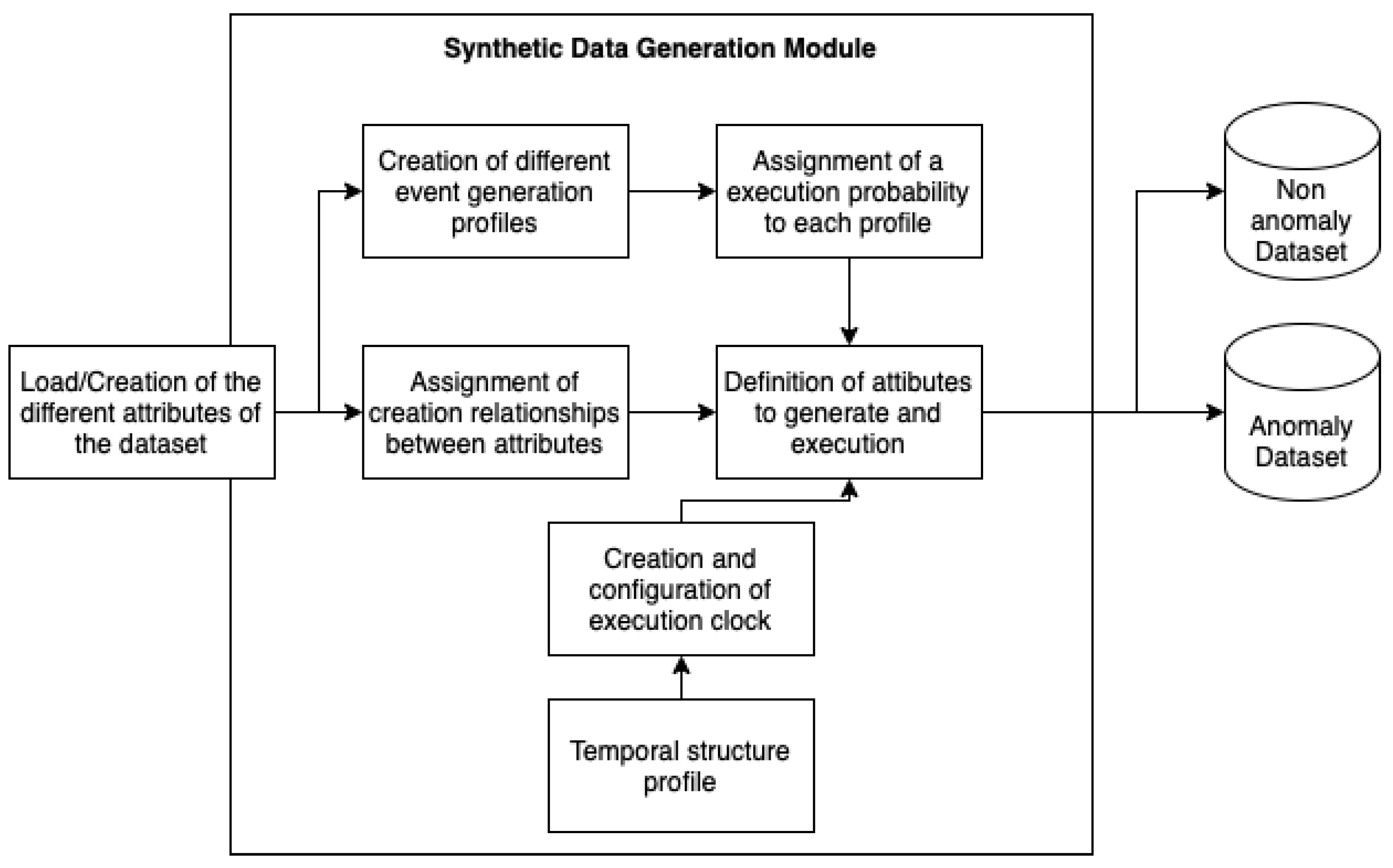
The architecture of the module is shown in
Figure 3.
The module uses the data provided from the inputs and establishes relationships between the attributes that are necessary for avoiding invalid inputs. In turn, profiles are defined to generate events by specifying the number of events that occur per clock step and then adding the probability that each profile will be executed per clock step.
This clock configuration is set in advance and specifies the simulation time and the time between steps. This configuration is conditioned by a time profile in which the characteristics of event generation are specified as a function of time (e.g., a higher number of steps during working time).
Finally, the attributes to be generated are defined with all configurations, relations and profiles. It should be noted that two different configurations are defined for the generation of a normal record and an anomalous record.
All these configurations are related to the library for the generation of realistic datasets Trumania [
38], which is a library that provides the necessary tools for the synthetic generation of data, the definition of the internal structures of the dataset and the prevention or enablement of the generation of events that meet the following requirements:
Suitable types for all values of the dataset that facilitate their subsequent modification;
Non-uniform structure for the generation of events;
Plausible time structure in relation to real normal and abnormal scenarios;
The impossibility of generating events that cannot occur in real environments.
The output data of the subsystem correspond to a pair of records generated with normal characteristics and a record with abnormal characteristics. The size of these created records is about 100,000 entries, and they can be varied in any order.
The characteristics of the generated datasets are identical to those generated and sent by the specific device with which we are up-sampling.
5.3. Preprocessing
This subsystem is responsible for normalising, transforming and standardising the values of the dataset before training the machine learning algorithms and real-time processing. Data preprocessing is defined in
Figure 4 and divided into the different modules that make it up.
The input data of this system consist of a set of data values from each device. This information is first structured according to the type of datum so that the type of datum is defined. This structuring process is performed by defining a schema at the beginning of the data load that contains names of the attributes of the device data to which it refers, followed by the definition of the type of value contained in these attributes [
39].
Then, preprocessing modules offered by Apache Spark and the respective functions defined for each type of event appear (String Indexer [
40], Min-Max Scaler [
41], Standard Scaler [
42], One Hot Encoder [
43], Hash Encoder [
44], Regex Tokenizer [
45], Count Vectorizer [
46], TF-IDF [
47], Word2Vec [
48] and Vector Assembler [
49]), performing relevant transformations and adjusting the data as a result. Some examples are presented in
Figure 5,
Figure 6,
Figure 7 and
Figure 8.
5.4. Training and Validation
The training and validation subsystem aims to generate machine learning models that enable the detection of possible anomalies based on the data from the devices described above. The training and validation subsystem consists of the following components:
The internal architecture of this subsystem is shown in
Figure 9.
The training and validation subsystem is responsible for preparing and monitoring the correct functioning of the machine learning model for anomaly detections. This is performed by using input data consisting of training data and validation data.
The training data are preprocessed by the preprocessing subsystem, which performs the above transformations depending on the type of event. For the identification of the best machine learning model for a given device type, hyperparameter selection modules, metrics and validation data are used.
The hyperparameter selection module is responsible for determining which feature set of a given machine learning model architecture is best suited for anomaly detection. Hyperparameters are selected based on the results provided by the metrics module. Therefore, the evaluation of the machine learning model for each set of devices is performed by the metrics module together with the validation dataset. This module allows the evaluation of the accuracy of an anomaly detection algorithm by applying a set of mathematical functions.
The mathematical functions chosen to determine the best hyperparameter for the model were the WSSSE metric and the Silhouette metrics used under the criterion of the ‘elbow point’ of the graph when selecting hyperparameters. It consist of plotting variations of the metric as we vary the hyperparameter value. From the graph, we select the point where the variation of the slope occurs.
Once the most accurate model has been obtained, the final model is determined for each device. The result, after going through the training and validation subsystem, is the different final models created for each device in the system.
5.4.1. Machine Learning Algorithm Threshold
The algorithms used to run the model to identify anomalies are the following: K-Means, bisecting K-Means and GMM. These algorithms allow the grouping of data into clusters of similar characteristics in an unsupervised manner.
The decision for one or the other algorithm is made after comparing the WSSSE and Silhouette metrics between the three models, as explained in the Results section.
The model with the best performance is selected, so the next step is to define the mechanism by which the model will detect an anomaly and a normal event. For this purpose, the models will use a threshold for each cluster formed. This allows us to define which data are sufficiently different from the rest of the cluster in order to be considered an anomaly.
Therefore, a model will be trained with a set of data that is considered non-anomalous so that, when new events are detected, whether these new data are similar enough to be detected as anomalies or not can be compared and observed.
The threshold is variable and can be more or less restrictive as needed. However, when defining the threshold, the default is to assign the distance greater than the furthest point from each centroid of the cluster to which it belongs.
In summary, the anomaly detection method works as follows:
Assigning the optimal hyperparameters for each model depending on WSSSE, silhouette and training time;
We compare the results of the metrics with each other and select the one with the best result;
The selected model is trained with the data from the dataset of events considered normal, creating different clusters and setting a threshold for each;
By default, the threshold is equal to the furthest point with respect to the centroid of the cluster to which it belongs. A threshold value is set for each cluster created. The value of the threshold can be changed as needed.
5.4.2. Selection of the Hyperparameters
The selection of hyperparameters in machine learning algorithms is crucial when designing the models to be implemented for each type of problem.
The method for choosing each hyperparameter was performed iteratively, testing a range of possible values and selecting the one that showed the best performance with the minimum number of clusters. This performance is represented in the WSSSE and Silhouette curves resulting from the iterative process performed on each hyperparameter and in the training time required for each of the models to be compared.
The metric that will be given more importance is Silhouette since it shows both the compactness of a cluster and the separation between clusters, while WSSSE only allows viewing the dispersion of the points of the clusters. In cases of similar Silhouettes, WSSSE will be observed and, in case it does not vary, training times will be analysed. In this paper, when analysing clustering algorithms, we will define the following hyperparameters in the three studied models. The results obtained are presented in
Table 2 for models with optimisations that can be completed.
The high computational cost of training with the bisecting K-Means clustering model automatically implies that it is rejected as a solution for this proposal.
5.5. Real-Time Processing
The real-time processing subsystem is responsible for processing data from the various devices and identifying possible anomalies. These anomalies are determined by machine learning algorithms that were previously obtained by the training and validation subsystem. The internal architecture of this subsystem is shown in
Figure 10.
The input data of the real time processing subsystem correspond to the set of data generated in real time by the set of devices. These input data are subscribed to Kafka, which manages the input stream data. This information is then sent to the pre-processing system, which is responsible for converting the input data into structured data in order to understand it properly.
Machine learning algorithms have been previously trained and validated in the corresponding subsystem to detect possible anomalies in the input data. In the real-time processing subsystem, there are several machine learning models for each type of device. The output data correspond to the result of the detection of normal or anomalous events. The trace with the values of the event itself and the result of the detection is stored in the “Anomalies” database with a unique identifier corresponding to the event.
6. Results
6.1. Model Comparison
The comparison of the three models associated with each of the devices is displayed after selecting the hyperparameters for each of them. The purpose of this comparison is to select the best model for each data source, taking into account the three metrics used: WSSSE, Silhouette and training time. For each of the three models per device, the same dataset and hardware/software environment was used to consider only the aspects related to the performance of the models themselves.
From the results presented in
Table 3, it appears that the K-Means model performs equally or similarly to the bisecting K-Means model in most cases, but improves training time significantly by a factor of 10.
The GMM model appears to be the worst. Most tests, given the results of the Silhouette metric, show that its performance is significantly inferior to both K-Means and bisecting K-Means. This can be explained by the fact that GMM tends to get caught in local minima, resulting in those Silhouette values. Nevertheless, the result in training time is similar to K-Means. Another advantage of K-Means over the other two models is that it does not suffer from convergence or training time problems that prevent its use in some models, as is the case with GMM and bisecting K-Means. So, the model that seems to work best for each device is K-Means; therefore, this model is used for anomaly detection.
6.2. Detection Ratio
To see how the system works and how powerful it is, three types of tests were conducted for each model connected to each device.
Seven different data sources were considered that provided activity data to be tested as follows:
Identification as normal data when the log represents non-anomalous activity;
Identification as possible anomalous data if information has never been seen before and it is sufficiently different from the training data.
For the test, two sets of samples are used for each device. The first set is considered as a normal set of samples and the second set of samples is considered anomalous.
Table 4 shows the result of measuring the accuracy of a system in an environment where normal data or data with possible anomalies have been defined. The result shows that almost all data considered normal and those with possible anomalies are classified as such.
It should be noted that all these results depend on the training and validation data provided/generated by each device. Although the data are promising, further testing is required to substantiate the results.
6.3. Cluster Visualisation
Another way to determine if the cluster creation performance is correct is to visualise the different clusters created by different models. They need to be shaped correctly as they are used in the threshold for anomaly detection.
Once the clustering process is completed, in order to avoid any interference and only for visualisation purposes, it is necessary to perform a dimension reduction process to represent them in one plane. For this, four types of dimension reducers were used (PCA, ISOMAP, t-SNE and UMAP). In
Figure 11, we show a visualisation where the clusters obtained with each model can be better identified after the dimension reduction process, abd we can verify that the anomalies are correctly detected by the model.
6.4. Comparison with Related Works
In
Section 2, we presented a relation of the previous works related to anomaly detection with different techniques in order to present the advantages of our proposal in relation to those results.
In
Table 5, we included our characteristics to be compared with the Related Works, highlighting that our system obtained high quality results with widespread techniques and including real-time processing, a study and the pre-processing of data collected by our devices.
7. Conclusions
Anomaly detection is a commonly addressed issue in recent cybersecurity research studies and is examined by various approaches. For the real-time processing of these incidents, unsupervised methods are very useful when the data that contain outliers are heterogeneous or specific for a certain device.
To do so, we have designed a real-time solution to deal with anomalies from various sources in a heterogeneous real environment.
After outlining all the modules and processes that make up the real-time anomaly detection system and conducting various tests with respect to its detection capability and performance, we were able to determine that the best algorithm among the proposed algorithms for tackling the threshold detection problem is K-Means, which is sometimes equivalent to bisecting K-Means, but it has better training times. GMM performed the worst and scored the lowest in the Silhouette metric. In the clusters obtained with K-Means, this configured threshold determines the difference between normal traffic and anomalies.
The conclusion drawn from the test conducted to check the system’s ability to detect anomalies is that the detection of normal events and anomalous events had an acceptable performance, with an accuracy metric close to 99%. The UEBA–Browsers model had the lowest results, which was 86% for anomaly detection, while Process is the most accurate at identifying anomalous logs.
Finally, testing the performance of an unsupervised learning model is more complex than for other paradigms. The fact that events are undefined with respect to which are anomalous and which are normal is a major obstacle in determining the performance of the model. This means that the results shown may vary if the execution conditions or the configuration of different models change.
In the development of the real use case presented in this paper, we found some limitations, such as the impossibility to complete hyperparameter optimisation in some models because they exceeded the defined runtime for meeting the real-time condition or the lack of real logs for some of the models, which we had to synthetically generate. These issues may be addressed in the continuation of this line of research.
Moreover, for future developments, improving the treatment of possible abnormal events by temporal features is proposed. Since it is difficult to integrate this type of detection with the others, spliting the models (for each data source) into two models is proposed so that one can detect anomalies using non-temporal features and another can detect anomalies using temporal features. For better control over the process, we would also implement a blacklist/whitelist mechanism with the models to manually narrow down which hours are anomalous for the operator. On the other hand, we would like to test the result of combining the outputs of multiple models, especially the result of combining K-Means with GMM since one of the biggest problems of GMM is that it gets stuck in the local minima, which could be solved by first running K-Means and then initialising GMM with the centroids given by K-Means. Eventually, this proposal could be integrated into a cyber situational awareness platform.


 ,
, 


