Intelligent Bearing Fault Diagnosis Based on Open Set Convolutional Neural Network

Abstract

Traditional data-driven intelligent fault diagnosis methods have been successfully developed under the closed set assumption (CSA). CSA-based fault diagnosis assumes that the fault types in the test set are consistent with that in the training set, which can achieve high accuracy, but this is generally not valid in real-world industrial applications where the collection of data in industrial applications is often limited. As it is unrealistic to assume that the training set will cover all fault types, the application of the fault classifier may fail when the test set contains unknown fault types because the probability of input samples belonging to unknown types cannot be obtained. To solve the problem of how unknown fault types may be accurately identified, this paper further studies the open set assumption (OSA) fault diagnosis. We propose an open set convolutional neural network (OS-CNN) method and apply our OS-CNN model to an improved OpenMax method as a deep network to accurately detect unknown fault types. The overall performance was significantly improved as our OS-CNN model was able to effectively tighten the boundary of known classes and limit the open-space risk for the OpenMax method based on distance modeling. The overall effectiveness of the proposed method was verified by experimental studies based on four different bearing datasets. Compared with state-of-the-art OSA fault diagnosis method, our method cannot only realize the correct classification of the known fault classes, but it can also accurately detect the unknown fault classes.

1. Introduction

Rolling element bearings in mechanical parts play a vital role [1] in the field of modern industrial machinery. According to relevant information, among the types of mechanical failures, about 30 percent of the faults are caused by the failure of rolling bearings. To avoid expensive maintenance costs, huge economic losses, and even life safety problems caused by the failure of mechanical parts, the technology of equipment condition monitoring and fault diagnosis based on vibration signals are widely concerned. At present, as a research hotspot in the field of mechanical fault diagnosis, many mature bearing fault diagnosis technologies have been formed in the actual scene.

In the 1990s, various shallow machine learning models were successively proposed, such as support vector machines (SVM), K-nearest neighbor (KNN), Bayesian classifiers, decision trees and artificial neural networks (ANN). These early efforts were instrumental in pushing fault diagnosis into the era of artificial intelligence. A number of intelligent fault diagnosis methods have emerged, including methods based on expert systems [2], methods based on neural networks (NNs) [3], methods based on SVM [4], and other artificial intelligent methods [5]. An important aspect of these shallow learning methods is that as they rely on manual feature selection to identify the health status of the machine, the quality of selected features become the bottleneck of the overall system performance. In contrast to traditional shallow learning, deep learning (DL) has the important capability of feature learning. DL directly learns from raw data by constructing a nonlinear neural network with multiple hidden layers which automatically extract features and abstract them layer by layer, thus mapping the samples from the original feature space to a new feature space which improves the accuracy of classification or prediction. This indicates that the "deep model" is the mean, and "feature learning" is the goal. Compared with traditionally manually constructed features, features learned by deep models can better capture the rich internal information in the data through feature learning. The DL models that are mainly used in the field of intelligent fault diagnosis include autoencoder (AE) [6,7], deep belief network (DBN) [8,9], convolutional neural network (CNN) [10,11], recurrent neural network (RNN), and deep residual network (DRN) [12]. Among these, deep intelligent fault diagnosis models based on CNN and AE are the most popular. Generally, these methods take advantage of the feature extraction of DL models, and connect a classifier to the last layer of DL models to realize fault diagnosis, such as SoftMax, SVM, random forest, etc.

Most current intelligent fault diagnosis models are DL methods based on the closed set assumption (CSA), which assumes that the fault types in the training and test data share the same class features. However, the methods under this assumption have superior fault detection performance in the field of fault diagnosis. Moreover, since the training set cannot contain all fault types, this assumption is not valid in practical industrial applications as it is often unrealistic or even impossible to ensure that the training set will contain all possible fault types. Firstly, manually labeling all fault types during the training phase is expensive can be error-prone. Secondly, the process of vibration signal collection is time-consuming, and it is difficult to collect all types of fault data in a limited time. Moreover, some types of fault may not even occur during training data collection. DL models based on the CSA will misclassify it into the fault type defined by the training set when a previously unseen type of fault appears in the test set. In order to solve this problem, it is necessary to develop an open set assumption (OSA)-based method for fault diagnosis that cannot only correctly classify the known classes (KCs) but can also identify the unknown class (UC). 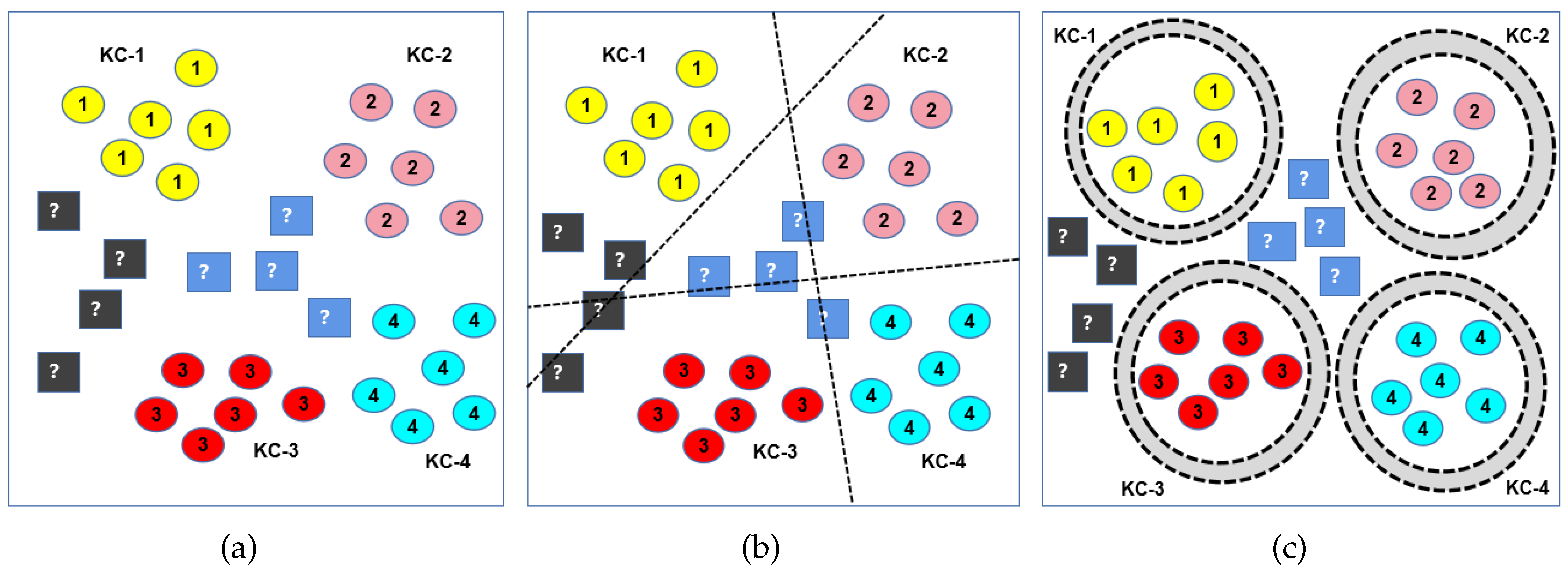Figure 1 provides a comparison between CSA and OSA classification. Figure 1a shows the distribution of the original dataset, including KC (labeled as 1, 2, 3, 4) and UC (labeled as ?). KC appears in both the training and testing phases, while UC only appears in the testing phase. As shown in Figure 1b,c, dotted lines and circles represent decision boundaries, respectively. The classifier classifies all points in the decision boundary into one class to divide different classes. Figure 1b shows that the traditional CSA classification method only considers the empirical risk and cannot deal with the open space risk. The classifier misclassifies the new category as KC, i.e., the existence of UC will introduce errors in classification decision making, so it is particularly important to limit the risk of open space. In contrast, as shown in Figure 1c, the decision boundaries of the OSA classification method is able to limit the range of KC(1, 2, 3, 4) and exclude UC(?). Hence, the UC(?) can be rejected instead of being misclassified as KC(1, 2, 3, 4). The OSA classification method combines empirical risk and open space risk which considers the space beyond the reasonable support of KCs. To improve the rejection ability of UC, it is necessary to further limit the open space risk and ensure that the open space risk is minimized.

The OSA-based classification method has been studied in many fields, mainly in the field of face recognition [13], security field [14], text classification [15,16], and network traffic [17], etc. However, there are few studies on OSA-based methods in the field of industrial bearings [18,19], and their experimental data are insufficient, so there is still much room to improve the rejection ability of UC. Therefore, it is urgent to explore a bearing fault diagnosis method based on OSA. This shows that research based on OSA classification methods is an extremely important development.

The main contributions of this paper can be summarized in the following three aspects:

(1)

A comprehensive experimental task is set up and applied to the field of OSA-bearing fault diagnosis, in which the test tag set includes all the training tag sets and UC. To make the experimental content more sufficient, this paper uses multiple combinations of four datasets, and proves the effectiveness of the method through 84 experiments. The experimental results exceed other state-of-the-art method results.

(2)

For the proposed OS-CNN model, the last layer uses multiple sigmoid functions to replace a single SoftMax function to limit the risk of open space, which has a certain novelty in the application of bearing fault diagnosis. The experiments show that this method is not only effective for the OSA problem but can also improve the convergence speed and the accuracy of final classification for the CSA problem.

(3)

By visualizing the distribution of the activation vectors of the penultimate layer of the bearing samples, it was found that the OpenMax method is insufficient in correcting the activation vectors. Since the distribution of the activation vectors is not all positive, the UC is misclassified as the KC. Based on this, this paper uses the exponential function to improve, so that the activation vector is above the positive value, i.e., the revised activation vector is more realistic. It is verified that the proposed method has better performance than the existing methods in identifying UC on four datasets.

The rest of this paper is organized as follows. Section 2 introduces the existing related work of the OSA. In Section 3, the OSA fault diagnosis method proposed in this paper is introduced in detail. In Section 4, the experimental settings of four datasets are described in detail and the experimental results are analyzed. The conclusions are drawn in Section 5.

2. Related Work

At present, there have been many studies based on the OSA classification problem. In terms of traditional machine learning methods such as SVM, Scheireret et al. [20] changed the traditional CSA, introduced a novel 1-vs.-set machine, and defined the combination of empirical risk and open risk as a constraint minimization problem, which was successfully applied to OSA classification. To further limit the open risk problem, Scheireret et al. [21] established a compact abating probability (CAP) model and considered nonlinear kernel functions, combining extreme value theory (EVT) [22] with two separate SVMs and proposed a Weibull-calibrated SVM (W-SVM) model. Jainet et al. [23] continued to use the EVT method to model the positive training samples of the decision boundary, thereby proposing the $P_I$-SVM algorithm. $P_I$-SVM limits open risk by using a threshold-based classification scheme, but the choice of threshold is also an issue. To solve this problem, Scherreiket et al. [24] introduced the probabilistic open set SVM (POS-SVM) classifier, which maps the output of SVM to probability. Based on minimizing the risk of an open set, the threshold is applied to determine whether the sample belongs to the training class or should be rejected, which provides better performance in distinguishing KCs from UC.

Since distance plays a vital role in limiting the open set risk, many classical methods were proposed in this area. Nearest class mean (NCM) [25] as a traditional distance method has many extensions. The method of nearest class mean metric learning (NCMML) [26] method extends the NCM approach, by using low-rank Markov distance instead of Euclidean distance to obtain better results. Bendale and Boult [27] proposed the nearest non-outlier (NNO) algorithm by extending the NCM classifier which can effectively evolve the model, detect outliers, and manage the risks of open space. Furthermore, Junioret et al. [28] further introduced an open set version of the nearest neighbor classifier (OSNN), which extended the nearest neighbor (NN) classifier by comparing the similarity threshold with the most similar class, and has good stability.

While DL was mostly used in traditional CSA, there have been explorations into the field of OSA with promising results. Traditional DL classifiers usually use SoftMax to calculate the classification probability, but this method cannot identify unknown samples and simply classify them as KCs. To solve this problem, Bendale and Boult [29] introduced a new model layer, OpenMax. Firstly, the penultimate activation vector value is extracted to calculate the average activation vector of each category, and the distance between it and the positive training sample is calculated. Then, the Weibull distribution of each class is obtained by distance fitting. The activation vector of the sample is further revised according to the Weibull distribution, and the calculation of the pseudo activation vector of UC is provided. Finally, the probability of the input sample belonging to a KC or UC is calculated. Shuet et al. [15] proposed a new method based on DL, which uses multiple sigmoid functions instead of the single SoftMax function in the last layer to limit the risk of open space. Kardan and Stanley [30] proposed a new standard neural network structure, called a competitive overcomplete output layer (COOL) neural network to solve the problem of the overgeneralization of neural networks in regions far from training data. Then, inspired by the OpenMax method, Prakhyaet et al. [16] studied the applicability of OpenMax in open set text classification and achieved good results in the classification of novel sample classes. Yoshihashi et al. [31] proposed the classification–reconstruction learning for open set recognition (CROSR). Its training network is used for joint classification and input data reconstruction, which is robust to UC detection without affecting the classification accuracy of KCs. Osa and Patel [32] proposed an open set recognition algorithm based on class conditioned auto-encoders, which adopted novel training and testing methods and used EVT to model reconstruction errors and to find the threshold to identify KCs or UC.

Given that the OSA method has made promising progress in other application domains, this paper designs an effective solution to the practical problem of OSA-bearing fault diagnosis.

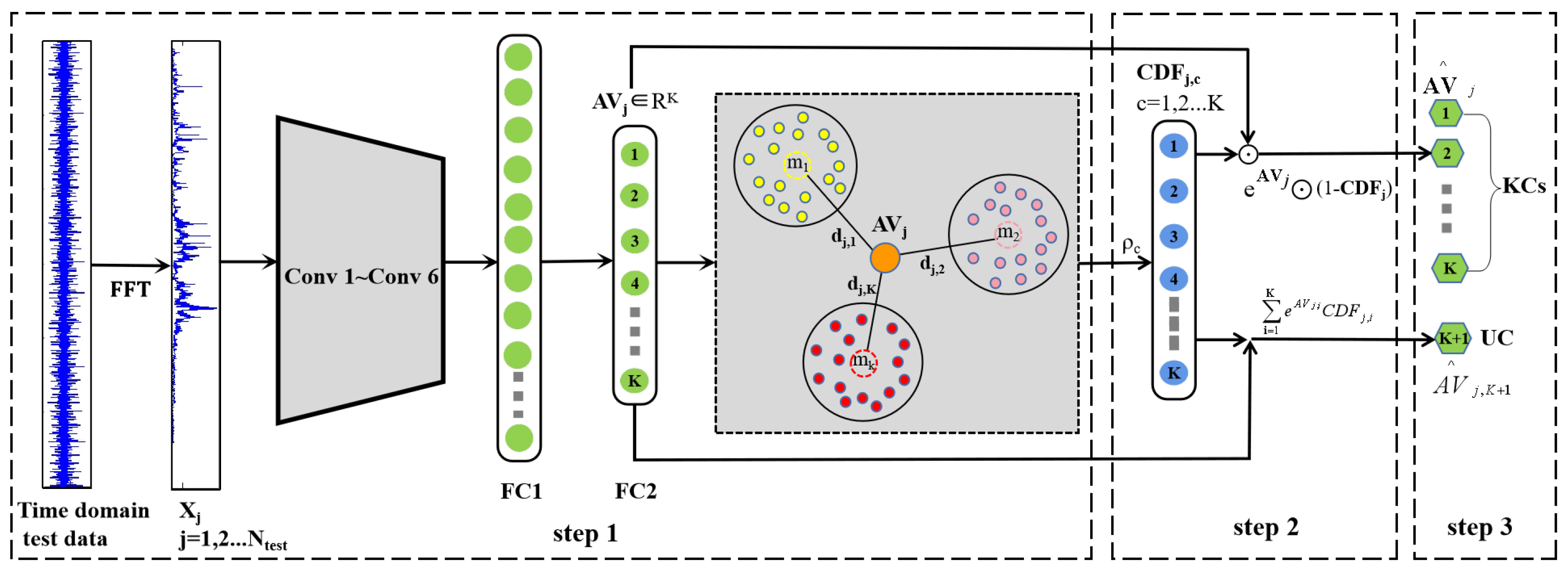
3. Method

3.1. Problem Description

Considering the actual industrial machinery application scenario, the training set and test set are not consistent. Bearing faults may occur on the inner ring, outer ring, ball, and cage, but fault symptoms (e.g., pitting, wear, and fracture) and fault sizes may be different. As a result, the fault type of the test phase is unpredictable and may contain one or more unknown fault modes. It is thus important that a practical fault diagnosis model has the ability to detect UC. This paper defines the OSA fault diagnosis problem as follows: the label sets of the training data contain K classes, called KCs, the label sets of the test data contain L classes, where K KCs defined in training set and $L-K$ UC, and all UC are classified as $(K+1)-th$ class. The dataset is defined as follows: the training data $D_{train}$ = $\left\{(x_1,y_1),...,(x_m,y_m)\right\}$ consist of m labeled data, $y_i(i=1,...,m)$ belongs to one of the K KCs, and the test data $D_{test}$ = $\left\{x_1,...,x_n\right\}$ consist of n unlabeled data. Our goal is that the classifier eliminates UC without reducing the classification accuracy of KCs, i.e., the shared tag sets are classified into K KCs, and the unknown sample is classified into $(K+1)-th$ class.

The method proposed in this paper is divided into the following three parts. Firstly, the overall framework of the OS-CNN model is described in detail, and its effectiveness is verified by comparison with other situations (Section 3.2). Secondly, it illustrates how to establish the Weibull model for known fault modes to measure the weight of abnormal class (Section 3.3). Finally, the test samples are input into the trained OS-CNN model to evaluate the Weibull distribution of the test samples for calculating the probability of belonging to K KCs and UC (Section 3.4).

3.2. Os-Cnn Architecture for Open Set Fault Diagnosis

Compared with traditional machine learning methods, CNN has strong learning ability and interpretability and has been widely used in the intelligent fault diagnosis of mechanical parts. The time-domain signals or frequency-domain signals after fast Fourier transform (FFT) [33,34] can be directly used as the input for CNN, without manual feature extraction to obtain more advanced results. For example, Ince et al. [35] directly inputted the original vibration signal into the 1DCNN model to detect motor faults, which greatly reduced the time-consuming and laborious in-feature extraction process. Sikder N. et al. [36] used the FFT to preprocess the original signal as the input of CNN, which revealed the inherent characteristics of the fault and obtained high precision. Zhang J. et al. [37] converted the original signal into the two-dimensional image as the input of CNN to automatically complete the feature extraction and fault diagnosis process, which meets the real-time requirements of bearing fault diagnosis. However, the current CNN method is mainly for the CSA problem. To solve the problem of the fault category during the test being unpredictable, this paper proposes an open set fault diagnosis model based on CNN, called OS-CNN.

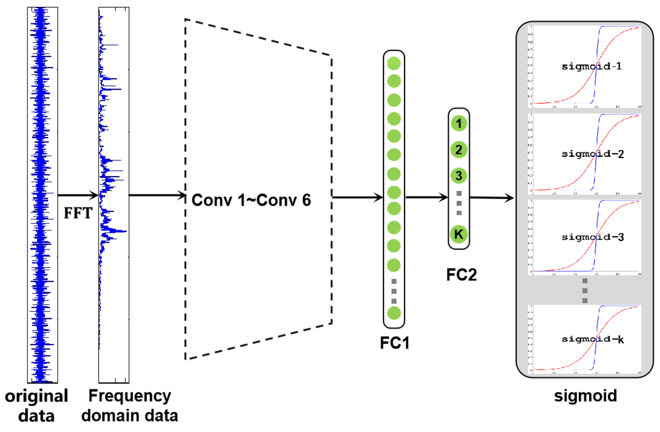
The architecture of OS-CNN is shown in Figure 2, which contains six convolution layers and pooling layers. The FC2 layer represents K class nodes, and the sigmoid layer represents K sigmoid functions corresponding to K KCs. To suppress the influence of high-frequency noise on classification accuracy in bearing signals, the OS-CNN structure proposed in the paper is similar to the WDCNN method proposed by Zhang et al. [38]. The first layer uses a wide convolution kernel. Specifically, the size of the first convolution kernel is $64\times 1$, and the size of the remaining kernels is $3\times 1$. The pooling type is maxpooling, and the activation function is ReLU. In order to normalize the data, a Batch Normalization (BN) layer is added after each convolution layer. Two fully connected (FC) layers are used behind the convolution layer, and the node in the second fully connected layer (FC2) corresponds to the fault type in the training set. The last layer of the model is inspired by the deep open classification (DOC) method [16], which builds a 1-vs.-rest layer containing K sigmoid functions for K KCs. The specific method seeks to establish K sigmoid functions for K KCs and then converts each KC into a probability distribution in the range of [0,1] to calculate the uncertainty measure for each class.

For m training samples in the training set $D_{train}$, each sample $x_i$ has a class label $y_i$, which contains K KCs, if the $l-th$ sigmoid function corresponds to the fault class $C_l$, i.e., $y_i$ = $C_l$ is a positive sample, the corresponding label is 1, all the remaining known faults are negative samples, and the corresponding label is 0, so each sigmoid function can construct a 1-vs.-rest training set. The model is trained with the sum of logarithmic losses corresponding to K sigmoid functions.

$$\begin{array}{cc}\hfill \mathrm{Loss}=& \sum _{l=1}^K\sum _{i=1}^m-\mathbb{I}\left(y_i=C_l\right)logp\left(y_i=C_l\right)\hfill \\ \hfill & -\mathbb{I}\left(y_i\ne C_l\right)log\left(1-p\left(y_i=C_l\right)\right),\hfill \end{array}$$

(1)

where $\mathbb{I}$ is the indicator function, its value is 1 if $y_i$ = $C_l$, otherwise 0. The $p\left(y_i=C_l\right)$ is the probability output of the $l-th$ sigmoid function on the $i-th$ training sample.

The parameters of each convolution layer and pooling layer are shown in

Table 1. Details of the feature extractor used in the experiments.

No.	Layer Type	Layer Name	Kernel	Stride	Channel	Output	Padding
1	Convolution	Conv1	64 × 1	2 × 1	16	125(253) × 16	Yes
	MaxPool		1 × 1	2 × 1	16	125(253) × 16	No
2	Convolution	Conv2	3 × 1	2 × 1	32	62(126) × 32	Yes
	MaxPool		1 × 1	2 × 1	32	62(126) × 32	No
3	Convolution	Conv3	3 × 1	2 × 1	64	30(62) × 64	Yes
	MaxPool		1 × 1	2 × 1	64	30(62) × 64	No
4	Convolution	Conv4	3 × 1	2 × 1	64	14(30) × 64	Yes
	MaxPool		1 × 1	2 × 1	64	14(30) × 64	No
5	Convolution	Conv5	3 × 1	2 × 1	64	6(14) × 64	Yes
	MaxPool		1 × 1	2 × 1	64	6(14) × 64	No
6	Convolution	Conv6	3 × 1	2 × 1	64	2(6) × 64	Yes
	MaxPool		1 × 1	2 × 1	64	2(6) × 64	No

.

3.3. Establish the Weibull Model for Known Fault Modes

To make the classifier accurately reject UC without reducing the classification accuracy of KCs, it is necessary to combine the experience risk and open space risk for OSA fault diagnosis. How to reduce the risk of open space is the continuous pursuit of OSA work. Scheirer et al. [20] introduced the concept of open space risk, which is defined as the risk related to the ‘far away’ known training sample.

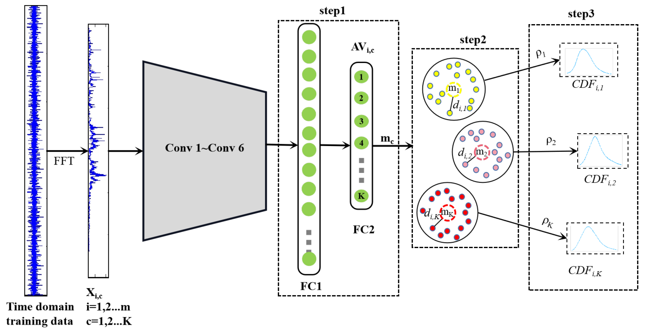
To adapt to bearing fault diagnosis based on OSA, this paper applies the OS-CNN deep network model to the OpenMax method. The OpenMax method considers the concept of open space risk and uses EVT to define a compact attenuation probability model. The distance distribution is evaluated by comparing the relationship between the input sample and the known training sample.

The OpenMax is different from the traditional method of calculating probability through the score of the last layer but uses the eigenvalues extracted from the penultimate layer (FC2) to estimate the distance. In this paper, the extracted value from the penultimate layer is called the activation vector (AV).

To facilitate the explanation, the OSA fault diagnosis method is divided into two processes (Section 3.3 and Section 3.4), each process including three steps.

The first process is divided into three steps as shown in Figure 3, where the solid black line at Conv1–Conv6 represents the trained model. The specific process for each step is as follows.

Step 1 

Input the labeled training data into the OS-CNN trained model and extract the AV corresponding to the positive training sample. Let ${\mathbf{AV}}_{i,c}$ denote the AV of the $i-th$ positive training sample of class c (c = 1,…,K) in the training set. Then, NCM is used to calculate the mean activation vector (MAV) corresponding to each KC, denoted as ${\mathbf{m}}_c$. The ${\mathbf{m}}_c$ can be expressed as:

$${\mathbf{m}}_c=mean\left({\mathbf{AV}}_{i,c}\right).$$

(2)

Step 2 

In order to evaluate the relationship between the input sample and the MAV of each class. The distance between the $i-th$ positive sample $x_i$ and the corresponding ${\mathbf{m}}_c$ is calculated, where the distance is denoted as $d_{i,c}$. As for the selection of distance calculation methods, three distance calculation methods on the bearing dataset are compared. They are the Euclidean distance method, the cosine distance method, and the combination of normalized Euclidean and cosine distances method, respectively. After experimental verification, the combination of normalized Euclidean distance and cosine distance can obtain the best performance. Therefore, the distance calculation adopts the combination of normalized Euclidean distance and cosine distances. The $d_{i,c}$ can be expressed as:

$$d_{i,c}=∥{\mathbf{AV}}_{i,c}-{\mathbf{m}}_c∥.$$

(3)

Step 3 

This paper estimates the distribution of each fault class based on the EVT method. Due to the EVT model following Weibull distribution, the libMR [39] FitHigh fitting function is used to perform Weibull fitting on the maximum distance between positive training samples and corresponding ${\mathbf{m}}_c$ to obtain the Weibull model parameters of each KC. The Weibull fitting parameter ${\rho }_c$ includes the shift ${\tau }_c$, shape ${\kappa }_c$, and scale ${\lambda }_c$, which is used to estimate the probability of outliers in the test phase. As shown in formula (4), the tail length ${\eta }_r$ is the selection of the $r-th$ maximum distance.

$${\rho }_c=\left({\tau }_c,{\kappa }_c,{\lambda }_c\right)=FitHigh\left(∥{\mathbf{AV}}_{i,c}-{\mathbf{m}}_c∥,{\eta }_r\right).$$

(4)

Then, the Weibull cumulative distribution function (CDF) is prepared for the next process to estimate the class of test samples. The corresponding $CD{F}_{i,c}$ is estimated by fitting parameter ${\rho }_c$ and distance $d_{i,c}$, which estimates the relationship between the $i-th$ training sample and $c-th$ class. The formula is shown in (5).

$$error=e^{-{\left(\frac{∥d_{i,c}-{\tau }_c∥}{{\lambda }_c}\right)}^{{\kappa }_c}},$$

(5)

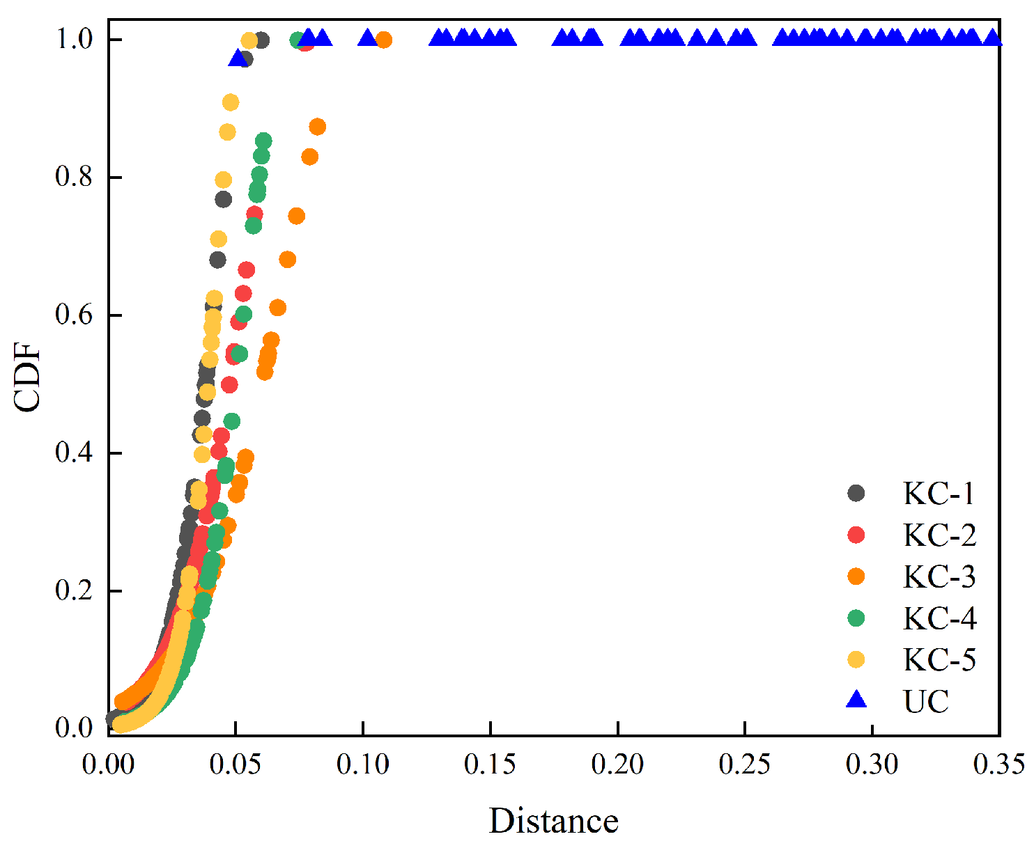
The $CD{F}_{i,c}$ probability distribution visualization is similar to the KCs distribution in Figure 4 of Section 3.4, where KC-1–KC-5 represent the distribution of KC training samples, and the blue triangle represents the distribution of unknown samples in the test phase. It can be found that the distribution of the known samples is a monotonically increasing function, with an increasing distance indicating a larger the CDF value.

3.4. Test Phase Based on the OS-CNN Algorithm

The process of the test phase is shown in Figure 5, where ⊙ denotes an element-wise product. It mainly includes the following three steps:

Step 1 

Input test data into the trained model, and the AV extracted from the $j-th$ test sample is denoted as ${\mathbf{AV}}_j$. The $d_{j,c}$ represents the distance between the $j-th$ test sample and the ${\mathbf{m}}_c$ of the $c-th$ KC to estimate whether the input is "far" from the known training data. The $d_{j,c}$ can be expressed as:

$$d_{j,c}=∥{\mathbf{m}}_c-{\mathbf{AV}}_j∥.$$

(6)

Step 2 

To evaluate the probability that the test samples belong to outliers, the value of $CD{F}_{j,c}$ is used to determine whether the test samples belong to the $c-th$ KC. Specifically, for the $j-th$ test sample, the distance $d_{j,c}$ and the corresponding fitting parameter ${\rho }_c$ are used to calculate the $CD{F}_{j,c}$, which measures the weight value of the input sample that does not belong to the $c-th$ KC, and serves as the core for estimating the rejection of the UC. To make the distribution of test samples more clear, the representative $CD{F}_{j,c}$ of test samples are selected for visualization. The distribution is shown in Figure 4, where the black dot test samples represent the distribution of $CD{F}_{j,1}$$(j=1,...,n)$ corresponding to the KC-1 node, i.e., it represents the distribution between the Weibull parameters of KC-1 and the distance from the KC-1 test sample to the first class of the feature center. Other KC samples are visualized in the same way. For the blue triangle test samples, the $CD{F}_{j,c}$ values calculated by the distance $d_{j,c}$ to each class of the feature center and the fitting parameter ${\rho }_c$ are concentrated near 1, indicating that it does not belong to any KC, and one group is selected for visualization.

Because UC is included in the test samples, there are $K+1$ classes in the test samples. The $(K+1)-th$ class represents the UC samples, but the OS-CNN model only has the output probability of K KCs. To calculate the probability that the input samples belong to KC and UC, the OpenMax method is used to revise the AV of input samples and further calculate the pseudo-AV of UC. Since the $CD{F}_{j,c}$ represents the weight of the input sample $x_j$ that does not belong to the $c-th$ KC, the $1-CD{F}_{j,c}$ measures the weight of the input sample $x_j$ belonging to the $c-th$ KC. To be specific, to determine whether the $j-th$ test sample belongs to the UC or not, the OpenMax method uses the ${\mathbf{AV}}_{\mathbf{j}}$ and $1-{\mathbf{CFD}}_{\mathbf{j}}$ corresponding element-wise product to calculate the revised AV. Hence, the revised AV for $c-th$ KC is close to 0 when $CD{F}_{j,c}$ is close to 1, indicating that the input sample is more likely to be UC, and the pseudo-AV of UC is expected to have a larger value.

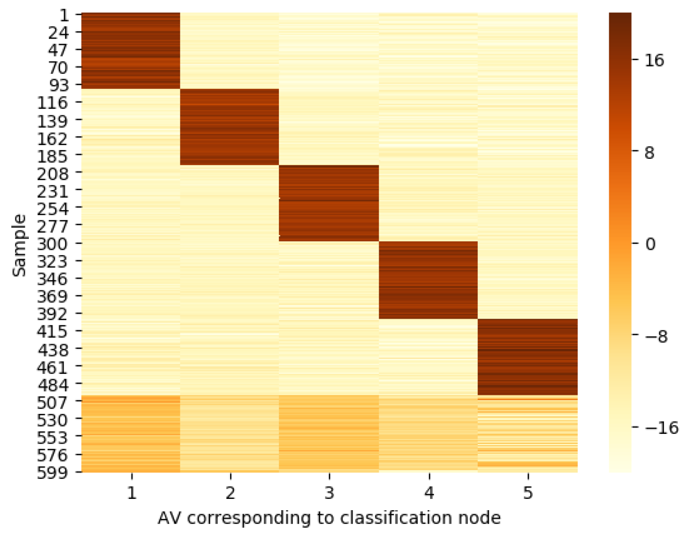
Although the OpenMax method obtained a superior result in [29], it is found that it is not suitable for bearing signals through experimental verification in this paper. Through multiple sets of experiments, it was found that the AV corresponding to the UC samples is not completely positive due to the characteristics of vibration signals, especially the quite clear data provided by the Case Western Reserve University (CRWU). As shown in Figure 6, 1–600 test samples correspond to the distribution of AV extracted from 5 KC nodes, of which 1–100 samples are KC-1, 101–200 samples correspond to KC-2, 201–300 samples are KC-3, 301–400 samples are KC-4, 401–500 samples are KC-5, and 501–600 samples are UC. As for the distribution of bearing signals, it can be seen that the AV distribution of the KC is relatively strong, and the AV extraction result of some UC is distributed in negative value. In this situation, if the input sample is a UC, its corresponding CDF value is close to 1, and the expected pseudo-AV of the UC is larger than the revised AV of the KCs. If we continue to use the OpenMax method to revise the AV, as shown in Formula (7), the revised AV of the $j-th$ test sample is denoted as ${\widehat{\mathbf{AV}}}_j$, and the pseudo-AV of the $j-th$ test sample is denoted as ${\widehat{AV}}_{j,k+1}$. Since the $A{V}_{j,i}$ corresponding to UC is negative, this will cause the pseudo-AV value $A{V}_{j,k+1}$ of UC to be negative. However, the revised AV value ${\mathbf{AV}}_{\mathbf{j}}$ of KCs is close to 0, resulting in the pseudo-AV of UC being smaller than the revised AV of KCs, which is inconsistent with expectations, and it is easy to misclassify UC as KCs.

$$\begin{array}{c}\widehat{\mathbf{AV}}{}_j={\mathbf{AV}}_j\odot \left(1-{\mathbf{CDF}}_j\right)\\ \widehat{A{V}_{j,k+1}}=\sum _{i=1}^{k}A{V}_{j,i}CD{F}_{j,i}\end{array}$$

(7)

Therefore, this paper improves the method [29] by using the exponential function to ensure the monotonicity of the extracted AV distribution and make it above the positive value.

The improved revised formula of AV is expressed as:

$$\begin{array}{cc}\hfill {\widehat{\mathbf{AV}}}_j& ={\mathbf{e}}^{{\mathbf{AV}}_j}\odot (1-{\mathbf{CDF}}_j)\hfill \\ \hfill {\widehat{AV}}_{j,k+1}& =\sum _{i=1}^k{e}^{A{V}_{j,i}}{CDF}_{j,i}\hfill \end{array}$$

(8)

Step 3 

After obtaining the revised AV, the probability value corresponding to each class is calculated to determine the category of each sample. However, UC appears in the test phase of the OSA scenario. As a result, it is contradictory to the probability sum of 1. To adapt the OpenMax method, the distribution probability of each test sample belonging to a certain KC and UC is calculated, as shown in Formula (9). The revised AV corresponding to each KC and the pseudo-AV of the UC are used as molecules, and its sum as a denominator, which meets the requirement of a probability sum of 1. Hence, the ability to reject input is provided when UC ($y=K+1$) has a maximum probability.

$$\widehat{P}(y=c\mid {\mathbf{x}}_j)=\frac{{\widehat{AV}}_{j,c}}{{\sum }_{i=1}^{k+1}{\widehat{AV}}_{j,i}}$$

(9)

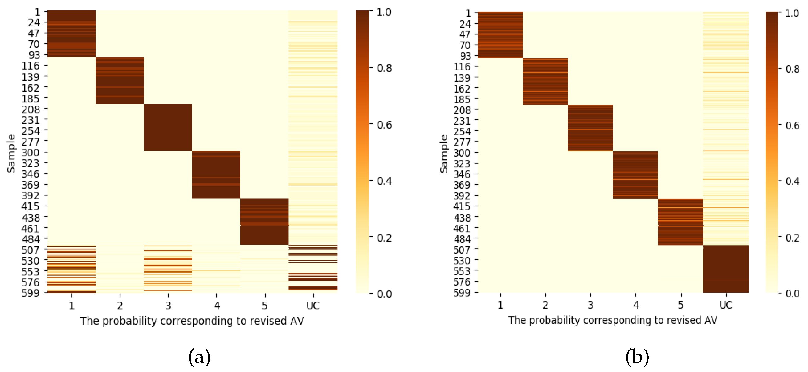
As shown in Figure 7a,b, this paper visualizes the probability value distribution of the revised AV before and after improvement. As shown in Figure 7a, it is easy to misclassify unknown samples into KCs. As shown in Figure 7b, it can clearly be seen that KCs and UC completed the correct distribution of KCs and UC, which verifies the effectiveness of the method used in this paper.

4. Experimental Results and Discussion

4.1. Dataset Description

This paper collects four different types of bearing datasets: the Case Western Reserve University (CWRU) dataset, Jiangnan University (JNU) dataset, Southeast University (SEU) dataset, and PHM2009 dataset. These datasets have specific labels and explanations. The detailed information is shown in Table 2, Table 3, Table 4 and Table 5.

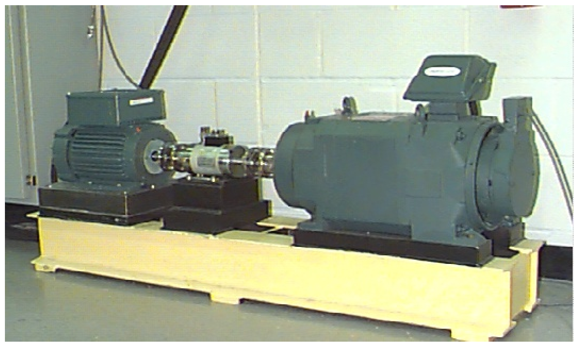
CWRU Bearing Dataset The basic layout of the test rig is shown in Figure 8. It consists of a 2 hp motor (left), a torque transducer/encoder (center), and a dynamometer (right). Further details regarding the test rig can be found on the CWRU Bearing Data Center website [40]. Vibration signals were collected from the drive end of a motor in the test rig under four different states: (1) normal condition (NO); (2) inner-race fault (IF); (3) outer-race fault (OF); and (4) ball fault (BF). For IF, OF, and BF cases, vibration signals for three different severity levels (0.007 inches, 0.014 inches, and 0.021 inches) were separately collected, respectively. The sampling frequency was 12 kHz and the signals were collected under four working conditions with different motor loads and rotating speeds, i.e., Load0 = 0 hp/1797 rpm, Load1 = 1 hp/1772 rpm, Load2 = 2 hp/1750 rpm and Load3 = 3 hp/1730 rpm. The CRWU dataset settings are shown in Table 2.

JNU Bearing Dataset The JNU bearing dataset was provided by Jiangnan University. The JNU dataset content can be downloaded from [41], and more detailed information can be obtained from [42]. It was collected at three different speeds of 600 rmp, 800 rmp, and 1000 rmp, and the acquisition frequency was 50 kHz. Each working condition included four bearing states: (1) NO; (2) IF; (3) OF; and (4) BF. More detailed information about the data description is shown in Table 3.

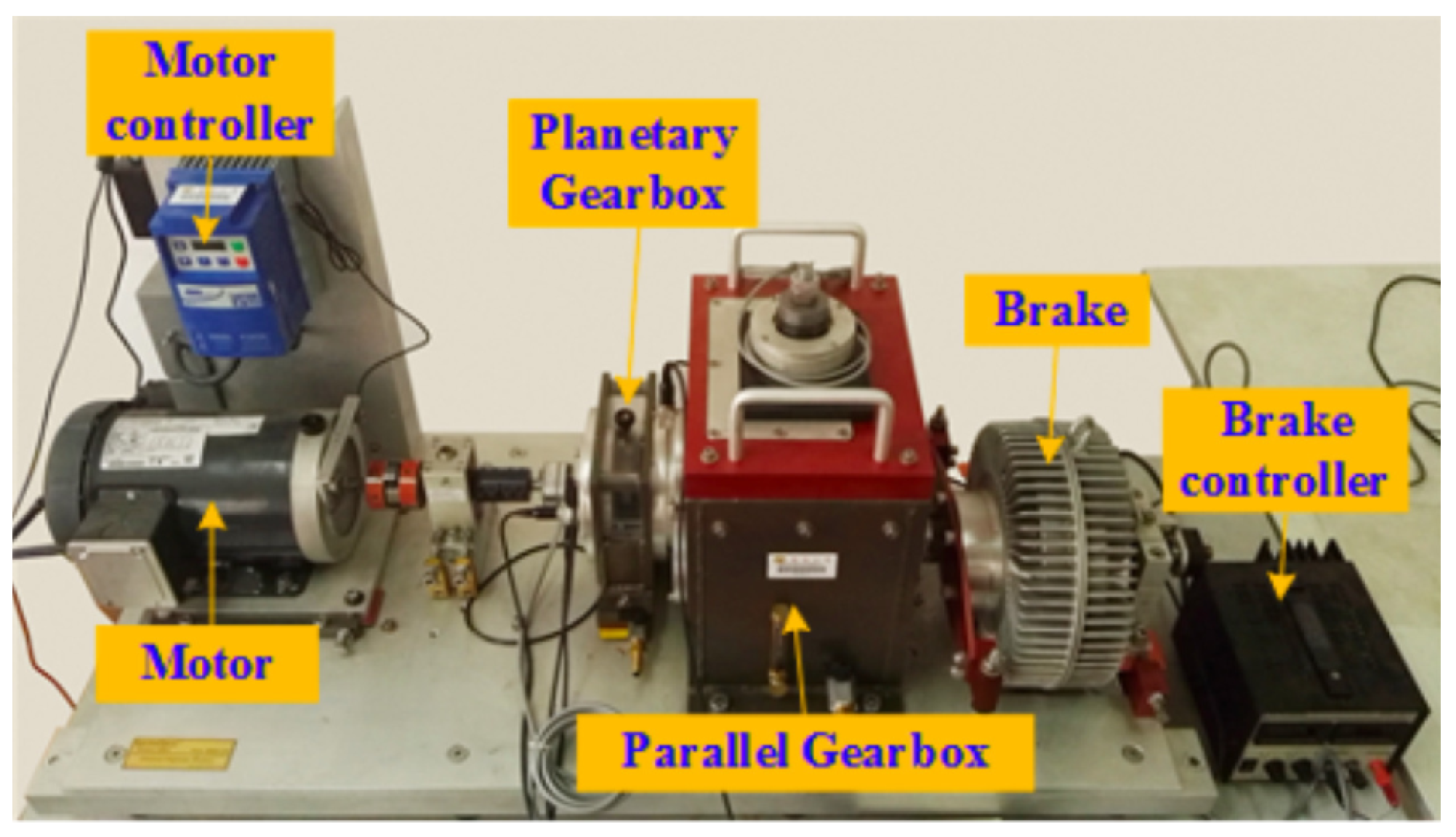
SEU Bearing Dataset The SEU gearbox dataset was provided by Southeast University. The whole experimental equipment is shown in Figure 9, with the dataset content available for download from [43] and more details from [44]. The dataset was acquired by the Dynamic Transmission System Dynamic Simulator (DDS), and contains two sub-datasets, namely the bearing dataset and the gear dataset. Under two different working conditions, the speed-load configuration (RS-LC, respectively) was set to 20 Hz-0 vs. and 30 Hz-2 v, and the vibration signal was collected at a frequency of 12 kHz. There were four bearing states under each operating condition: (1) NO; (2) IF; (3) OF; and (4) BF. In each file, there were eight lines of vibration signal, whilst this paper uses the second line of vibration signals. The basic layout of the experimental setup is shown in Figure 9. Details are shown in Table 4.

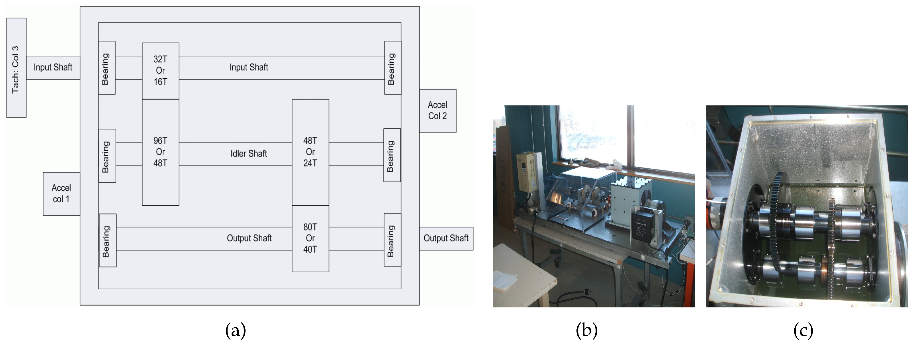
PHM2009 Bearing Dataset The PHM2009 gearbox fault data were representative of generic industrial gearbox data, which contain three shafts, four gears, and six bearings. For each health condition, the data were synchronously collected by the accelerometer installed on the input and output shaft mounting plates at 30 Hz, 35 Hz, 40 Hz, 45 Hz, and 50 Hz shaft speed under high and low load, with a sampling frequency of 66.67 kHz and an acquisition time of 4 s [45]. The dataset category consists of six different fault conditions. The schematic of the gearbox used to collect the data is shown in Figure 10. The PHM2009 dataset more detailed information can be obtained from [46]. In this paper, only the input channel of the vibration signals of the helical gearbox under low load is used to evaluate the capability of the proposed method [47]. The PHM2009 dataset settings are shown in Table 5.

4.2. Evaluation Metrics

This section presents the evaluation criteria used for the dataset and detailed experimental results.

In order to evaluate the performance of the proposed method in OSA scenarios, the diagnosis results of KCs, UC and comprehensive performance corresponding to each task were mainly evaluated. In the following experiments, this paper named the classification result of KC as K and the diagnosis result of UC as U. Their results represent the accuracy of the tests and the ability to reject unknown samples. Moreover, the $F{1}_{score}$ was used as a comprehensive evaluation standard, which was the harmonic average of P and R, representing accuracy and recall rate, respectively. The definition is

$$F{1}_{score}=2\times \frac{P\times R}{P+R\prime }$$

(10)

where P represents the actual number of positive samples in the predicted positive samples; R indicates how many of the positive samples are correctly predicted. For the multi-class classification task in this paper, the evaluation of $F{1}_{Macro}$ was renamed $F1$. The final multi-class classification comprehensive evaluation result $F1$ was obtained by calculating the P and R of each class and averaging them. The formula is expressed as

$$F1=\frac{1}{n+1}\sum _{i=1}^{n+1}{\left(F{1}_{\mathrm{score}}\right)}_i.$$

(11)

4.3. Experimental Setup and Parameter Settings

The original time-domain vibration data are first converted into the frequency domain by FFT. The main reason is that the frequency domain information is usually more sensitive to the health status of the machine and can generally obtain better fault diagnosis performance. For the CWRU dataset, JNU dataset, and SEU dataset, a vibration signal with a length of 4098 is originally selected from the original signals, and then FFT is executed to generate 4098 Fourier coefficients. Since the coefficients are symmetrical, each sample has 2049 coefficients. For the PHM2009 dataset, the vibration signals are first divided into 6144 sampling points as data segments [48], and then FFT is performed to generate 4097 coefficients for each sample [47].

To verify the effectiveness of the proposed method, this paper sets multiple tasks to evaluate the ability of the proposed method to detect and classify test samples. Each task includes a training set and a test set. The training set is the labeled KCs, and the test set is the unlabeled data, including KCs and UC. The multi-task settings of the four datasets are as follows: the training set of the CWRU dataset is set based on the absence of fault type and fault size. The first three tasks lack a fault type, i.e., IF, OF or BF. The last three tasks lack a fault size, i.e., they are missing a fault size of 7 inches, 14 inches, or 21 inches. The training sets of the JNU, SEU, and PHM2009 datasets are based on the lack of one or two or three fault categories, respectively. The test set is unlabeled data, including training label set and UC that do not appear in the training set. In all task experiments, 70 percent of the training set is used for training, and the remaining samples are used for testing to evaluate the performance of the training model. It is worth noting that because the number of training set samples for all tasks is not consistent, the given batch size is 32 when the number of training set samples is large, and the batch size given is 16 when the number of training samples is small.

The task setting details of each dataset are shown in the following Table 2, Table 3, Table 4 and Table 5.

Table 2. The information of the CWRU and specific task settings.

Dataset	Class Label	0	1	2	3	4	5	6	7	8	9
CWRU	Fault Type	NO	IF	IF	IF	BF	BF	BF	OF	OF	OF
	Fault Size (Inches)	0	7	14	21	7	14	21	7	14	21
	Load (hp)	0, 1, 2, 3
Task	Experimental setup	Training label set					Test label set
C0	Missing fault type	0, 1, 2, 3, 4, 5, 6					0, 1, 2, 3, 4, 5, 6, 7, 8, 9
C1		0, 1, 2, 3, 7, 8, 9					0, 1, 2, 3, 4, 5, 6, 7, 8, 9
C2		0, 4, 5, 6, 7, 8, 9					0, 1, 2, 3, 4, 5, 6, 7, 8, 9
C3	Missing fault size	0, 1, 2, 4, 5, 7, 8					0, 1, 2, 3, 4, 5, 6, 7, 8, 9
C4		0, 2, 3, 5, 6, 8, 9					0, 1, 2, 3, 4, 5, 6, 7, 8, 9
C5		0, 1, 3, 4, 6, 7, 9					0, 1, 2, 3, 4, 5, 6, 7, 8, 9

Table 2. The information of the CWRU and specific task settings.

Dataset	Class Label	0	1	2	3	4	5	6	7	8	9
CWRU	Fault Type	NO	IF	IF	IF	BF	BF	BF	OF	OF	OF
	Fault Size (Inches)	0	7	14	21	7	14	21	7	14	21
	Load (hp)	0, 1, 2, 3
Task	Experimental setup	Training label set					Test label set
C0	Missing fault type	0, 1, 2, 3, 4, 5, 6					0, 1, 2, 3, 4, 5, 6, 7, 8, 9
C1		0, 1, 2, 3, 7, 8, 9					0, 1, 2, 3, 4, 5, 6, 7, 8, 9
C2		0, 4, 5, 6, 7, 8, 9					0, 1, 2, 3, 4, 5, 6, 7, 8, 9
C3	Missing fault size	0, 1, 2, 4, 5, 7, 8					0, 1, 2, 3, 4, 5, 6, 7, 8, 9
C4		0, 2, 3, 5, 6, 8, 9					0, 1, 2, 3, 4, 5, 6, 7, 8, 9
C5		0, 1, 3, 4, 6, 7, 9					0, 1, 2, 3, 4, 5, 6, 7, 8, 9

Table 3. The information of the JNU and specific task settings.

Dataset	Class Label	0	1	2	3
JNU	Fault Type	NO	IF	BF	OF
	Fault Speed (rmp)	600, 800, 1000
Task	Experimental setup	Training label set		Test label set
J0	An unknown class	0, 1, 2		0, 1, 2, 3
J1		0, 2, 3		0, 1, 2, 3
J2		0, 1, 3		0, 1, 2, 3
J3	Two unknown classes	0, 1		0, 1, 2, 3
J4		0, 2		0, 1, 2, 3
J5		0, 3		0, 1, 2, 3

Table 3. The information of the JNU and specific task settings.

Dataset	Class Label	0	1	2	3
JNU	Fault Type	NO	IF	BF	OF
	Fault Speed (rmp)	600, 800, 1000
Task	Experimental setup	Training label set		Test label set
J0	An unknown class	0, 1, 2		0, 1, 2, 3
J1		0, 2, 3		0, 1, 2, 3
J2		0, 1, 3		0, 1, 2, 3
J3	Two unknown classes	0, 1		0, 1, 2, 3
J4		0, 2		0, 1, 2, 3
J5		0, 3		0, 1, 2, 3

Table 4. The information of the SEU and specific task settings.

Dataset	Class Label	0	1	2	3
SEU	Fault Type	NO	IF	OF	BF
	RS-LC	20 Hz-0 V, 30 Hz-2 V
Task	Experimental setup	Training label set		Test label set
S0	An unknown class	0, 1, 2		0, 1, 2, 3
S1		0, 2, 3		0, 1, 2, 3
S2		0, 1, 3		0, 1, 2, 3
S3	Two unknown classes	0, 1		0, 1, 2, 3
S4		0, 2		0, 1, 2, 3
S5		0, 3		0, 1, 2, 3

Table 4. The information of the SEU and specific task settings.

Dataset	Class Label	0	1	2	3
SEU	Fault Type	NO	IF	OF	BF
	RS-LC	20 Hz-0 V, 30 Hz-2 V
Task	Experimental setup	Training label set		Test label set
S0	An unknown class	0, 1, 2		0, 1, 2, 3
S1		0, 2, 3		0, 1, 2, 3
S2		0, 1, 3		0, 1, 2, 3
S3	Two unknown classes	0, 1		0, 1, 2, 3
S4		0, 2		0, 1, 2, 3
S5		0, 3		0, 1, 2, 3

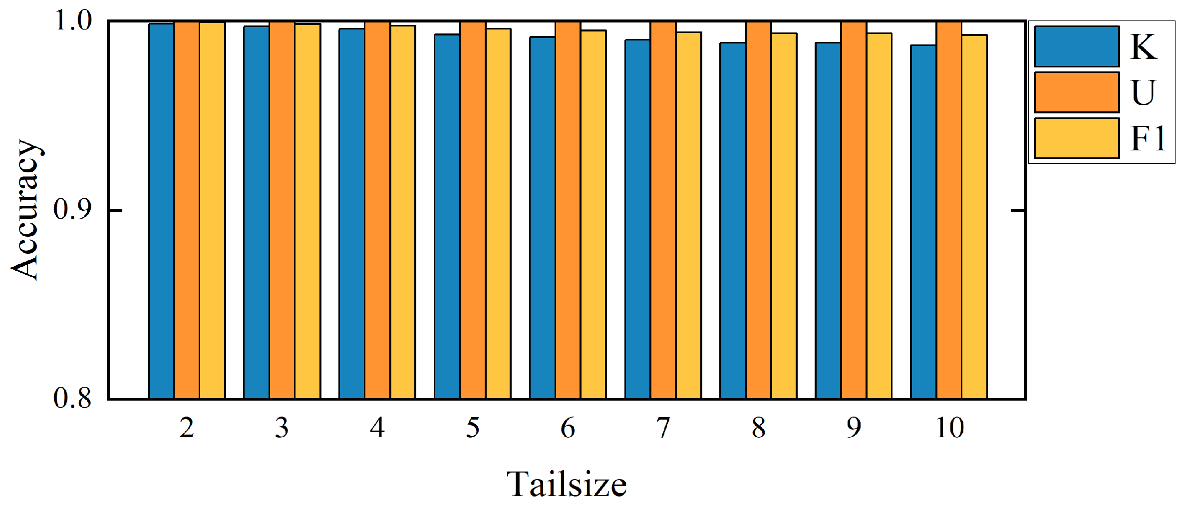
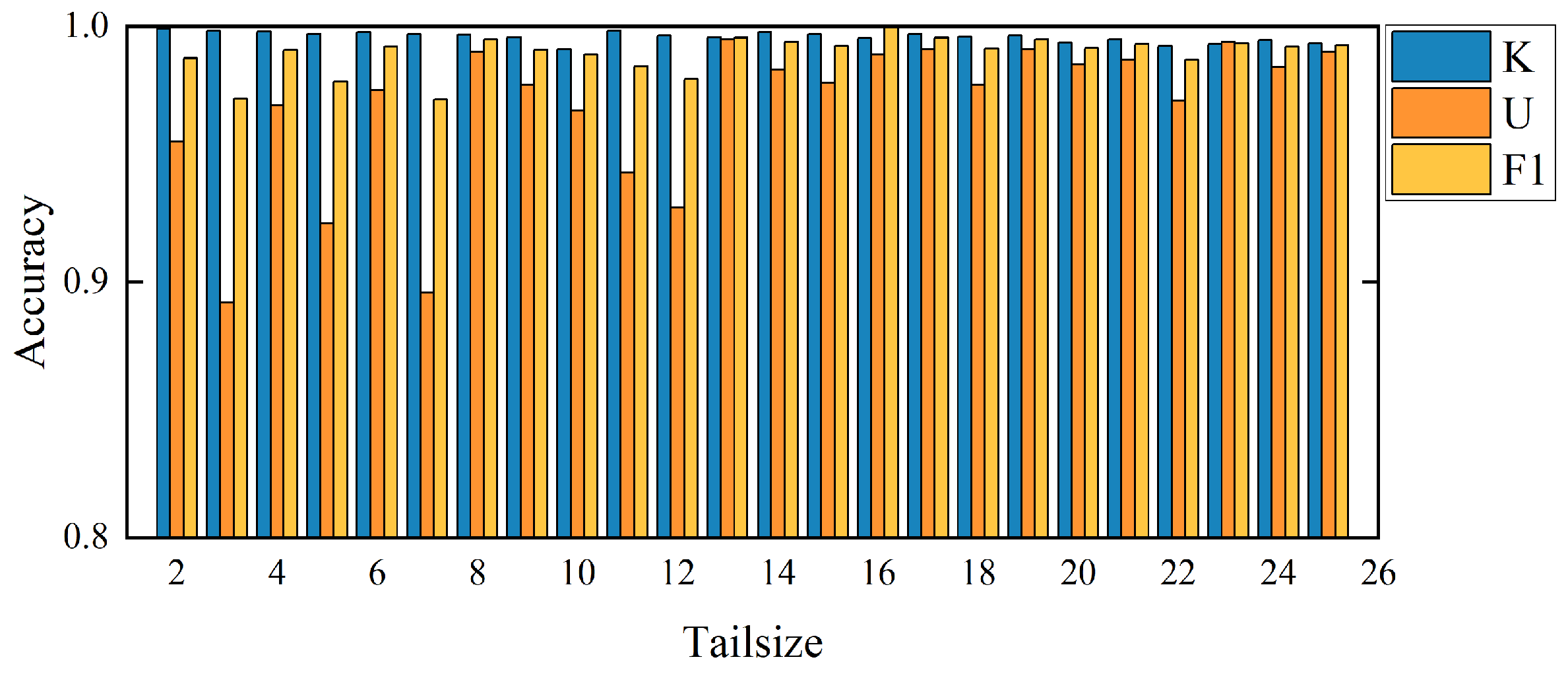
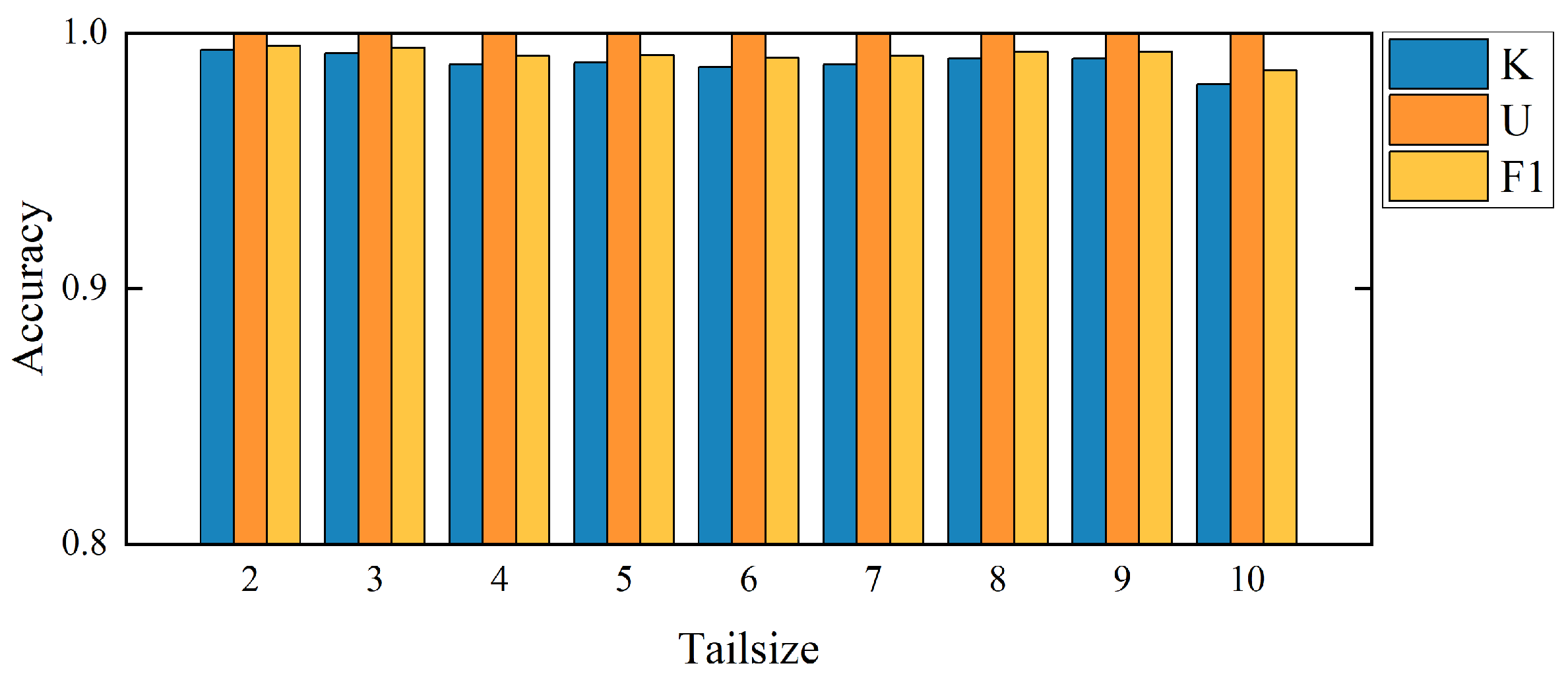
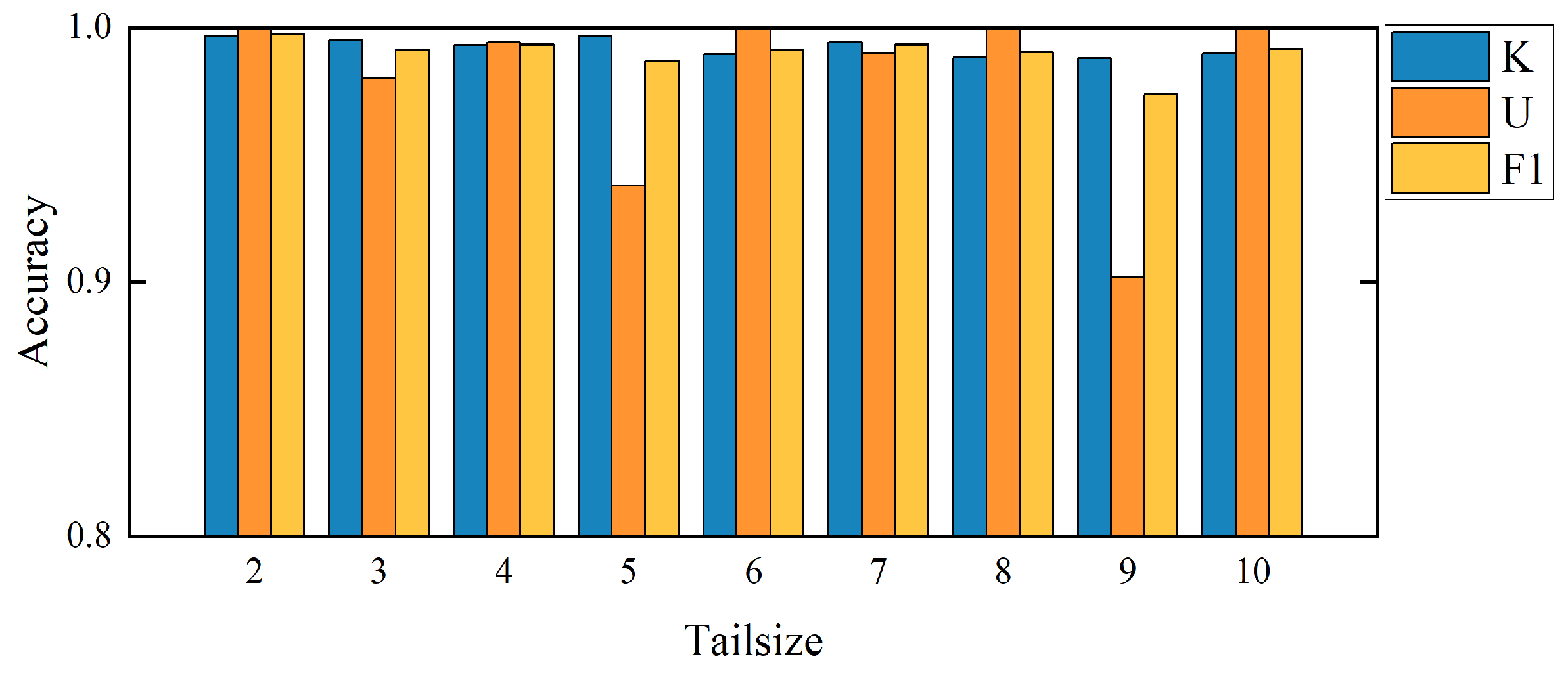
Due to the importance of the Weibull distribution calculation, the setting of tail size (Tailsize) length is critical for the experimental results. When Tailsize = 1, it does not conform to the distribution, so the experiment starts with Tailsize = 2 in this paper. After a large number of experiments on each dataset, this paper gives the accuracy histogram corresponding to a different Tailsize in each dataset to obtain the optimal selection of Tailsize corresponding to each dataset. For the CWRU dataset, the SEU dataset, and the PHM09 dataset, the best performance can be obtained when Tailsize = 2. For the JNU dataset, the best performance can be obtained when Tailsize = 23. The specific results of a different Tailsize corresponding to each dataset are shown in Figure 11, Figure 12, Figure 13 and Figure 14.

Table 5. The information of the PHM2009 and specific task settings.

Category	Gear		Bearing			Shaft
Labels	24T	Others	Input Shaft:Output Side	Idler Shaft:Output Side	Others	Input	Output
0	Good	Good	Good	Good	Good	Good	Good
1	Chipped	Good	Good	Good	Good	Good	Good
2	Broken	Good	Combination	Inner	Good	Bent Shaft	Good
3	Good	Good	Combination	Ball	Good	Imbalance	Good
4	Broken	Good	Good	Inner	Good	Good	Good
5	Good	Good	Good	Good	Good	Bent shaft	Good
Task	load		Experimental setup	Training label set		Test label set
p0			An unknown class	0, 1, 2, 4, 5		0, 1, 2, 3, 4, 5
p1				0, 1, 3, 5		0, 1, 2, 3, 4, 5
p2	ALL (30 hz, 35 hz,		Two unknown class	0, 1, 4, 5		0, 1, 2, 3, 4, 5
p3	40 hz, 45 hz, 50 hz)			0, 1, 5		0, 1, 2, 3, 4, 5
p4			Three fault class	0, 1, 4		0, 1, 2, 3, 4, 5
p5				0, 3, 5		0, 1, 2, 4, 5, 6

Table 5. The information of the PHM2009 and specific task settings.

Category	Gear		Bearing			Shaft
Labels	24T	Others	Input Shaft:Output Side	Idler Shaft:Output Side	Others	Input	Output
0	Good	Good	Good	Good	Good	Good	Good
1	Chipped	Good	Good	Good	Good	Good	Good
2	Broken	Good	Combination	Inner	Good	Bent Shaft	Good
3	Good	Good	Combination	Ball	Good	Imbalance	Good
4	Broken	Good	Good	Inner	Good	Good	Good
5	Good	Good	Good	Good	Good	Bent shaft	Good
Task	load		Experimental setup	Training label set		Test label set
p0			An unknown class	0, 1, 2, 4, 5		0, 1, 2, 3, 4, 5
p1				0, 1, 3, 5		0, 1, 2, 3, 4, 5
p2	ALL (30 hz, 35 hz,		Two unknown class	0, 1, 4, 5		0, 1, 2, 3, 4, 5
p3	40 hz, 45 hz, 50 hz)			0, 1, 5		0, 1, 2, 3, 4, 5
p4			Three fault class	0, 1, 4		0, 1, 2, 3, 4, 5
p5				0, 3, 5		0, 1, 2, 4, 5, 6

4.4. Experimental Results on Datasets

Table 6 shows the classification accuracy of the four datasets on different tasks. To reduce the potential influence of random results, all experimental results were averaged for 10 trials.

(1)

Results Analysis on Different Datasets

Based on the literature, the CWRU dataset is generally easier to diagnose faults with relatively distinct features. However, the PHM09 dataset is more practical and challenging, and there is significant signal noise in the condition monitoring data of other datasets relative to the CWRU dataset. As a result, the test accuracy of other datasets is lower than that of the CWRU dataset.

The classification accuracy of the six tasks in the CWRU dataset is shown in Table 6. It can be seen that the classification accuracy of the proposed method in this paper is more than 99% for KCs, and the detection accuracy of UC reaches 100%. In other words, the recognition of KCs also achieves good results when unknown data can be fully recognized. Experimental results show that the method used in this paper outperforms other existing methods in each diagnostic task of CWRU data. The experimental results of the JNU dataset on six tasks are shown in Table 7, the classification results of KCs are close to 100%, and the classification results of UC are all above 92%. Similarly, the experimental results of the SEU dataset on six tasks are shown in Table 8, and it can be seen that the classification accuracy of KCs is nearly 99% on all diagnostic tasks. The detection accuracy of UC under different tasks is higher than 99% except that the S2 task under 20HZ-0V is close to 94%. Compared with the results of other methods, the proposed method is more advanced. The experimental results of the PHM2009 dataset on six tasks are shown in Table 9, the classification accuracy for KCs is close to 100%, and the recognition accuracy results for UC are mostly above 90%. However, there are a few tasks in which the recognition of UC does not achieve the expected results. For example, the detection result of task 4 for UC is approximately 55% in the case of working condition 45 HZ, and the detection result of task 4 for UC is approximately 60% in the case of working condition 50 HZ. More detailed results can be viewed in the table. Based on the results of the above datasets, the effectiveness of the proposed method is verified.

From the above experiments, it can be observed that in the OSA task, our proposed method is not only able to effectively identify UC, but it also does not affect the classification accuracy of KCs. The experimental results validated the effectiveness of the proposed method. However, the results of a few tasks have shown some volatility or randomness. Therefore, there is still a need to explore more robust open set detection algorithms or improvements in the future.

(2)

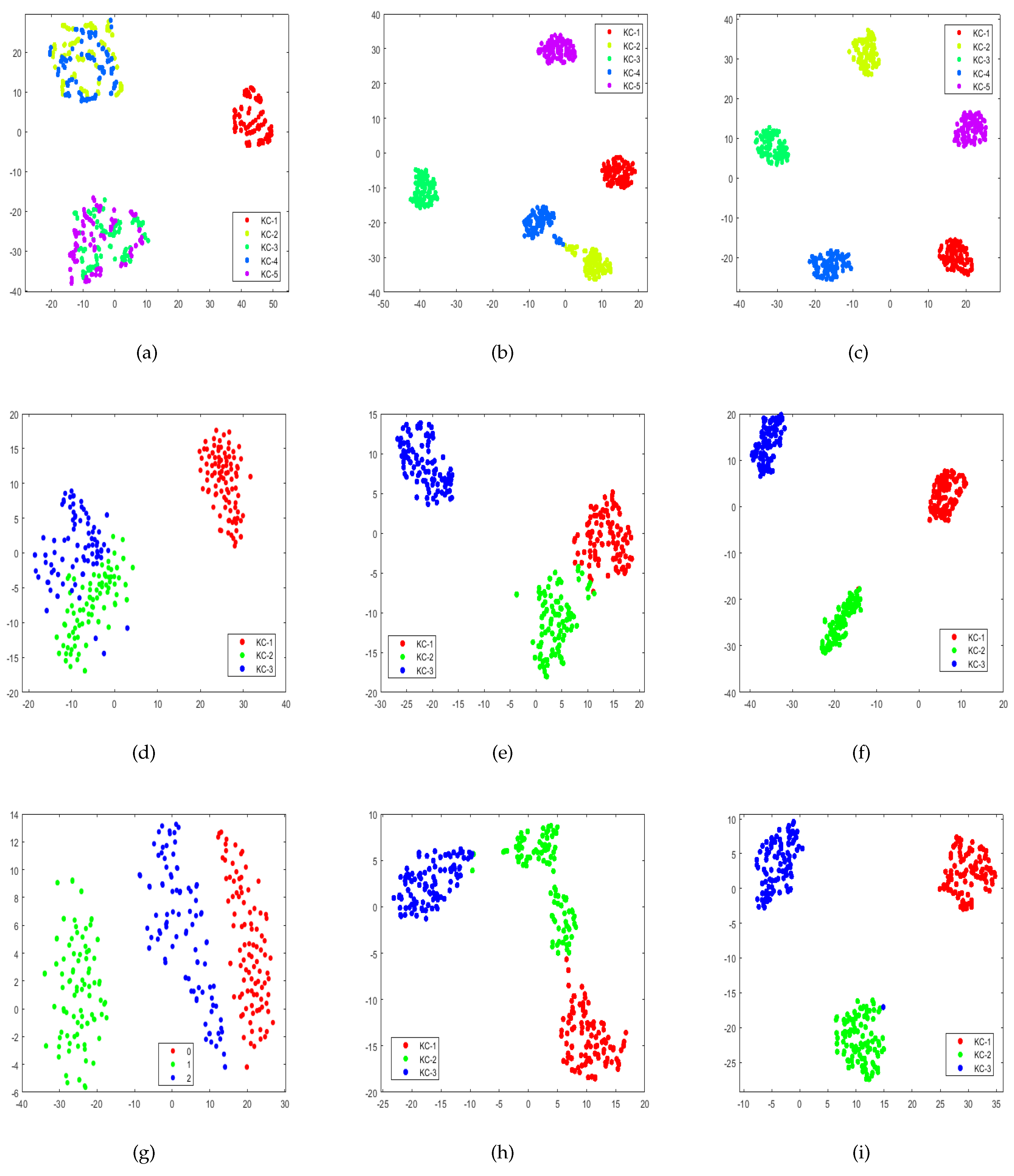
Feature Visualization

In order to intuitively observe the performance of the proposed CNN architecture, this paper uses the t-SNE visualization method to compare three situations on a task of PHM09 (a), (b), and (c), JNU (d), (e), and (f), and SEU (g), (h), and (i) datasets. The (a), (d), and (g) show FFT data visualization. The (b), (e), and (h) show that the last layer of the model uses the SoftMax function to visualize the eigenvalues extracted from the FC2 layer. The (c), (f), and (i) show that the last layer of the model uses a sigmoid function to visualize the eigenvalues extracted from the FC2 layer. The specific description of the dataset is shown in Table 5. In the first situation, FFT data are directly used for visualization. As shown in Figure 15a, the sample points of KC-2 and KC-3, KC-4 and KC-5 are mixed, respectively. In the second situation, FFT data are processed by the traditional CNN with a SoftMax layer. As illustrated in Figure 15b, although this method can correctly distinguish most samples, there is a small overlap between KC-3 and KC-4 samples. In the third situation, the last layer of the model consists of five 1-vs.-rest classifiers. It can be found that the KCs are completely classified in Figure 15c. The visualization results of the other two datasets also showed similar results. Furthermore, the method adopts multiple sigmoid functions instead of a single SoftMax function, which can make the distance between samples within the same fault type smaller and the distance between different fault types larger—effectively reducing the risk of open space.

Table 6. Experimental results of the CRWU dataset.

Task/Condition	0 hp			1 hp			2 hp			3 hp
	K	U	F1	K	U	F1	K	U	F1	K	U	F1
C0	0.9993	1.0000	0.9996	0.9994	1.0000	0.9997	0.9997	1.0000	0.9998	0.9993	1.0000	0.9996
C1	0.9993	1.0000	0.9996	0.9996	1.0000	0.9997	0.9996	1.0000	0.9997	0.9994	1.0000	0.9997
C2	0.9996	1.0000	0.9997	0.9993	1.0000	0.9996	0.9993	1.0000	0.9996	0.9996	1.0000	0.9997
C3	0.9999	1.0000	0.9999	0.9993	1.0000	0.9996	0.9997	1.0000	0.9998	0.9999	1.0000	0.9999
C4	0.9996	1.0000	0.9997	0.9993	1.0000	0.9996	0.9994	1.0000	0.9997	0.9994	1.0000	0.9997
C5	0.9993	1.0000	0.9996	0.9993	1.0000	0.9996	0.9994	1.0000	0.9997	0.9993	1.0000	0.9996

Table 6. Experimental results of the CRWU dataset.

Task/Condition	0 hp			1 hp			2 hp			3 hp
	K	U	F1	K	U	F1	K	U	F1	K	U	F1
C0	0.9993	1.0000	0.9996	0.9994	1.0000	0.9997	0.9997	1.0000	0.9998	0.9993	1.0000	0.9996
C1	0.9993	1.0000	0.9996	0.9996	1.0000	0.9997	0.9996	1.0000	0.9997	0.9994	1.0000	0.9997
C2	0.9996	1.0000	0.9997	0.9993	1.0000	0.9996	0.9993	1.0000	0.9996	0.9996	1.0000	0.9997
C3	0.9999	1.0000	0.9999	0.9993	1.0000	0.9996	0.9997	1.0000	0.9998	0.9999	1.0000	0.9999
C4	0.9996	1.0000	0.9997	0.9993	1.0000	0.9996	0.9994	1.0000	0.9997	0.9994	1.0000	0.9997
C5	0.9993	1.0000	0.9996	0.9993	1.0000	0.9996	0.9994	1.0000	0.9997	0.9993	1.0000	0.9996

Table 7. Experimental results of the JNU dataset.

Task/Condition	600 rmp			800 rmp			1000 rmp
	K	U	F1	K	U	F1	K	U	F1
J0	0.9990	0.9990	0.9990	0.9990	0.9850	0.9955	0.9987	0.9940	0.9975
J1	0.9983	0.9820	0.9942	0.9987	0.9810	0.9940	0.9975	0.9980	0.9944
J2	0.9940	1.0000	0.9955	0.9940	1.0000	0.9955	0.9967	1.0000	0.9975
J3	0.9865	0.9565	0.9729	0.9995	0.9840	0.9919	0.9990	0.9589	0.9767
J4	0.9990	0.9580	0.9790	0.9995	0.9425	0.9721	0.9995	0.9220	0.9621
J5	0.9985	0.9330	0.9671	0.9980	0.9910	0.9951	0.9995	0.9975	0.9985

Table 7. Experimental results of the JNU dataset.

Task/Condition	600 rmp			800 rmp			1000 rmp
	K	U	F1	K	U	F1	K	U	F1
J0	0.9990	0.9990	0.9990	0.9990	0.9850	0.9955	0.9987	0.9940	0.9975
J1	0.9983	0.9820	0.9942	0.9987	0.9810	0.9940	0.9975	0.9980	0.9944
J2	0.9940	1.0000	0.9955	0.9940	1.0000	0.9955	0.9967	1.0000	0.9975
J3	0.9865	0.9565	0.9729	0.9995	0.9840	0.9919	0.9990	0.9589	0.9767
J4	0.9990	0.9580	0.9790	0.9995	0.9425	0.9721	0.9995	0.9220	0.9621
J5	0.9985	0.9330	0.9671	0.9980	0.9910	0.9951	0.9995	0.9975	0.9985

Table 8. Experimental results of the SEU dataset.

Task/Condition	20 Hz-0 V			30 Hz-2 V
	K	U	F1	K	U	F1
S0	0.9897	1.0000	0.9923	0.9900	1.0000	0.9925
S1	0.9900	1.0000	0.9925	0.9900	0.9940	0.9910
S2	0.9887	0.9440	0.9773	0.9903	1.0000	0.9928
S3	0.9940	0.9975	0.9958	0.9980	0.9970	0.9975
S4	0.9890	0.9915	0.9903	0.9935	0.9910	0.9923
S5	0.9975	0.9990	0.9982	0.9967	0.9994	0.9981

Table 8. Experimental results of the SEU dataset.

Task/Condition	20 Hz-0 V			30 Hz-2 V
	K	U	F1	K	U	F1
S0	0.9897	1.0000	0.9923	0.9900	1.0000	0.9925
S1	0.9900	1.0000	0.9925	0.9900	0.9940	0.9910
S2	0.9887	0.9440	0.9773	0.9903	1.0000	0.9928
S3	0.9940	0.9975	0.9958	0.9980	0.9970	0.9975
S4	0.9890	0.9915	0.9903	0.9935	0.9910	0.9923
S5	0.9975	0.9990	0.9982	0.9967	0.9994	0.9981

Table 9. Experimental results of the PHM2009 dataset.

Task/ Condition	30 HZ			35 HZ			40 HZ			45 HZ			50 HZ
	K	U	F1	K	U	F1	K	U	F1	K	U	F1	K	U	F1
P0	0.9976	1.0000	0.9980	0.9956	1.0000	0.9964	0.9950	1.0000	0.9959	0.9922	0.9340	0.9825	0.9958	0.9980	0.9962
P1	0.9976	1.0000	0.9986	0.9983	1.0000	0.9989	0.9970	0.9975	0.9975	0.9960	1.0000	0.9976	0.9958	0.9900	0.9945
P2	0.9993	1.0000	0.9836	0.9985	0.9430	0.9826	0.9983	0.9125	0.9738	0.9950	0.8085	0.9439	0.9983	0.7653	0.9338
P3	0.9987	0.9977	0.9982	0.9967	0.9957	0.9962	0.9987	0.9917	0.9909	0.9637	0.8663	0.9136	0.9970	0.9903	0.9938
P4	0.9977	0.9277	0.9660	0.9993	0.9287	0.9663	0.9996	0.7440	0.8838	0.9993	0.5493	0.8023	0.9993	0.6040	0.8243
P5	0.9997	0.9987	0.9992	0.9987	0.9863	0.9927	0.9990	0.8990	0.9536	0.9993	0.7267	0.8874	0.9990	0.8563	0.9357

Table 9. Experimental results of the PHM2009 dataset.

Task/ Condition	30 HZ			35 HZ			40 HZ			45 HZ			50 HZ
	K	U	F1	K	U	F1	K	U	F1	K	U	F1	K	U	F1
P0	0.9976	1.0000	0.9980	0.9956	1.0000	0.9964	0.9950	1.0000	0.9959	0.9922	0.9340	0.9825	0.9958	0.9980	0.9962
P1	0.9976	1.0000	0.9986	0.9983	1.0000	0.9989	0.9970	0.9975	0.9975	0.9960	1.0000	0.9976	0.9958	0.9900	0.9945
P2	0.9993	1.0000	0.9836	0.9985	0.9430	0.9826	0.9983	0.9125	0.9738	0.9950	0.8085	0.9439	0.9983	0.7653	0.9338
P3	0.9987	0.9977	0.9982	0.9967	0.9957	0.9962	0.9987	0.9917	0.9909	0.9637	0.8663	0.9136	0.9970	0.9903	0.9938
P4	0.9977	0.9277	0.9660	0.9993	0.9287	0.9663	0.9996	0.7440	0.8838	0.9993	0.5493	0.8023	0.9993	0.6040	0.8243
P5	0.9997	0.9987	0.9992	0.9987	0.9863	0.9927	0.9990	0.8990	0.9536	0.9993	0.7267	0.8874	0.9990	0.8563	0.9357

4.5. Comparison Methods

In this section, we verifiy the effectiveness and superiority of the proposed method by comparing the performances of 1DCNN+EVT [18], DVAEC [19], and DOC [16] as reported in their corresponding literature. Table 10 shows the comparative results on four experimental tasks of the CWRU dataset in the literature [18]. The experimental results show that our method is better than other methods in the three evaluation indicators, especially for the recognition of UC, and can achieve a detection accuracy of almost 100% for all four tasks. In short, our method showed superior performance in terms of both KC classification accuracy and UC detection accuracy.

Table 11 shows the evaluation results of experiments on three experimental scenarios of the SEU dataset in the paper [19]. The speed load configuration of the SEU dataset was set to 30Hz-2V. The experimental results, in terms of the evaluation indicator F1, are compared with the three state-of-the-art methods in the literature [19]. We achieved the same performance in scenario 2. For the experimental results of the other two scenarios, the proposed method is superior to the standard detection method and can achieve 99% accuracy.

Table 10. Novelty detection performance of CRWU.

Tasks	1DCNN+KNN			1DCNN+SVDD			OpenMax			1DCNN+EVT			Proposed
	ALL	ALL*	UNK	ALL	ALL*	UNK	ALL	ALL*	UNK	ALL	ALL*	UNK	ALL	ALL*	UNK
C0	74.0	82.1	58.2	88.1	93.5	77.4	89.4	99.0	71.7	95.0	96.9	91.4	99.6	99.4	1.0
C1	87.1	92.3	66.6	94.0	96.5	84.5	93.3	99.0	84.0	97.7	97.7	98.1	99.6	99.4	1.0
C2	78.5	96.0	35.3	89.0	99.6	62.7	90.6	99.0	70.5	90.4	98.9	69.4	99.6	99.4	1.0
C3	80.4	87.7	55.5	88.6	96.0	63.5	96.0	99.0	90.0	91.3	95.0	78.5	99.5	99.2	1.0
Average	80.0	89.5	53.9	89.9	96.4	70.0	92.3	99.0	79.1	93.6	97.1	84.4	99.6	99.4	1.0

Table 10. Novelty detection performance of CRWU.

Tasks	1DCNN+KNN			1DCNN+SVDD			OpenMax			1DCNN+EVT			Proposed
	ALL	ALL*	UNK	ALL	ALL*	UNK	ALL	ALL*	UNK	ALL	ALL*	UNK	ALL	ALL*	UNK
C0	74.0	82.1	58.2	88.1	93.5	77.4	89.4	99.0	71.7	95.0	96.9	91.4	99.6	99.4	1.0
C1	87.1	92.3	66.6	94.0	96.5	84.5	93.3	99.0	84.0	97.7	97.7	98.1	99.6	99.4	1.0
C2	78.5	96.0	35.3	89.0	99.6	62.7	90.6	99.0	70.5	90.4	98.9	69.4	99.6	99.4	1.0
C3	80.4	87.7	55.5	88.6	96.0	63.5	96.0	99.0	90.0	91.3	95.0	78.5	99.5	99.2	1.0
Average	80.0	89.5	53.9	89.9	96.4	70.0	92.3	99.0	79.1	93.6	97.1	84.4	99.6	99.4	1.0

Table 11. Novelty detection performance of SEU.

Tasks	OCSVM	CAE	OpenMax	DVAEC	Proposed
	F1	F1	F1	F1	F1
Scenario 1	0.35	0.86	0.97	0.99	0.99
Scenario 2	0.41	0.77	0.98	0.80	0.98
Scenario 3	0.43	0.65	0.98	0.87	0.99
Average	0.40	0.76	0.98	0.89	0.99

Table 11. Novelty detection performance of SEU.

Tasks	OCSVM	CAE	OpenMax	DVAEC	Proposed
	F1	F1	F1	F1	F1
Scenario 1	0.35	0.86	0.97	0.99	0.99
Scenario 2	0.41	0.77	0.98	0.80	0.98
Scenario 3	0.43	0.65	0.98	0.87	0.99
Average	0.40	0.76	0.98	0.89	0.99

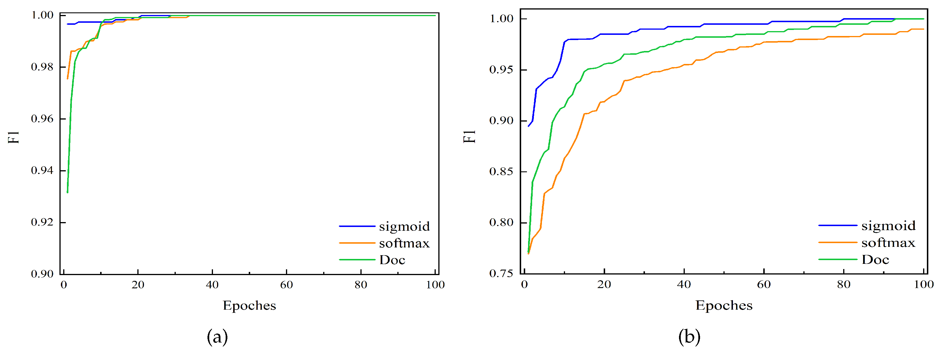
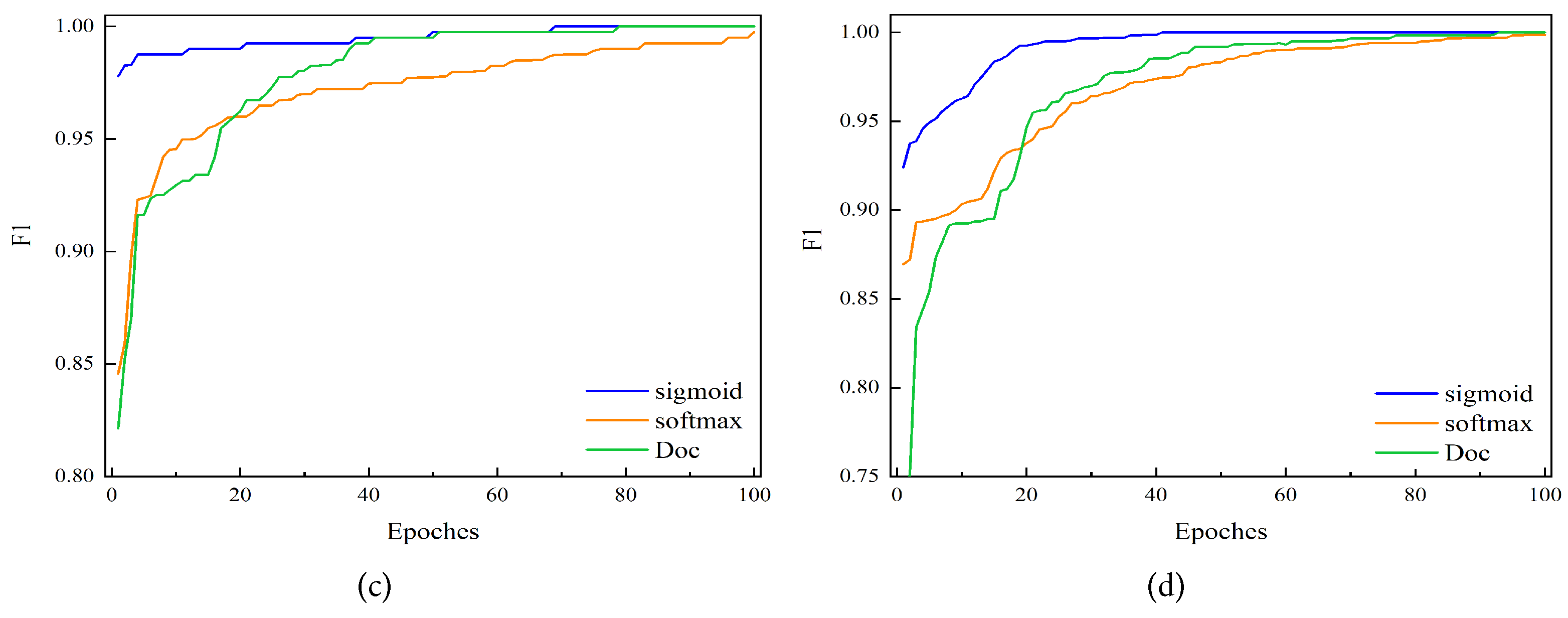
To further verify the performance of the proposed method, we also implemented the code of the DOC method [16] in the literature. Figure 16 shows that the comprehensive results of three different methods are compared on four datasets. The first method (shown in blue) used multiple sigmoid functions to replace a single SoftMax function at the last layer of the model and then applied it to the improved OpenMax method, i.e., the method proposed in this paper. The second method (shown in orange) used SoftMax function as the output layer of the last layer of the model. The third method (shown in green) used DOC, and to ensure the consistency of the experiment, CNN in the DOC method is modified to the model proposed in this paper. It can be seen from Figure 16 that our proposed method not only has better accuracy but also has better convergence than the other two methods in the comprehensive result F1. This shows that the proposed method noticeably outperforms those of the other two methods, which further verifies the superiority of our proposed method for OSA-based bearing fault diagnosis. The code is implemented in https://github.com/zccguess/OS-CNN.

5. Conclusions

This paper proposed an open-set bearing fault diagnosis algorithm based on OS-CNN, which solves the problem of the practical need to effectively identify new fault categories in the actual industrial environment. Extensive experimental results on four bearing datasets demonstrated that our proposed method provides more accurate diagnosis results than state-of-the-art OSA methods for rolling bearing fault. Overall, our proposed method not only accurately detects UC, but also ensures the accuracy of KC classification results. As the real-world scenarios of bearing fault diagnosis can be much more complex than what we considered in this paper, our proposal can be further improved through the following aspects. First, as our experiments were carried out under a single working condition, it is necessary to extend the proposed method to work under multiple working conditions. Second, in addition to UC detection, for practical usage, we also need to develop further methods for the model library to be continuously updated through expert marking and incremental learning, to realize the continuous detection ability without retraining.