
Representative Points from a Mixture of Two Normal Distributions

Abstract
:1. Introduction
2. Mixtures of Two-Component Normal Distributions
- If , , X follows a scale mixture, denoted as ;
- If , , X follows a location mixture, denoted as .
3. MSE-RPs from a MixN
4. Numerical Approximations to MSE-RPs from a MixN
4.1. The k-Means Algorithm
4.2. The Fang-He Algorithm
- Step 1. Set an initial value .
- Step 2. Solve the 1st equation in (10) to obtain by the bisection method or the iterative Newton’s method.
- Step 3. Solve the 2nd equation in (10) to calculate based on the values of and obtained in Steps 1 and 2.
- Step 4. Given the values of and , solve the equation in (10) to get for .
- Step 5. Given the solution of the equation, solve the equation in (10) to obtain another solution of .
- Step 6. Modify the initial value of and repeat the above procedure untilwhere represents the error tolerance, which is a very small number.
- If , the desired solution set is obtained.
- If , the initial value of is too small. Let , and go back to Step 1.
- If , the initial value of is too large. Let , and go back to Step 1.
5. Numerical Studies
5.1. Algorithm Comparisons
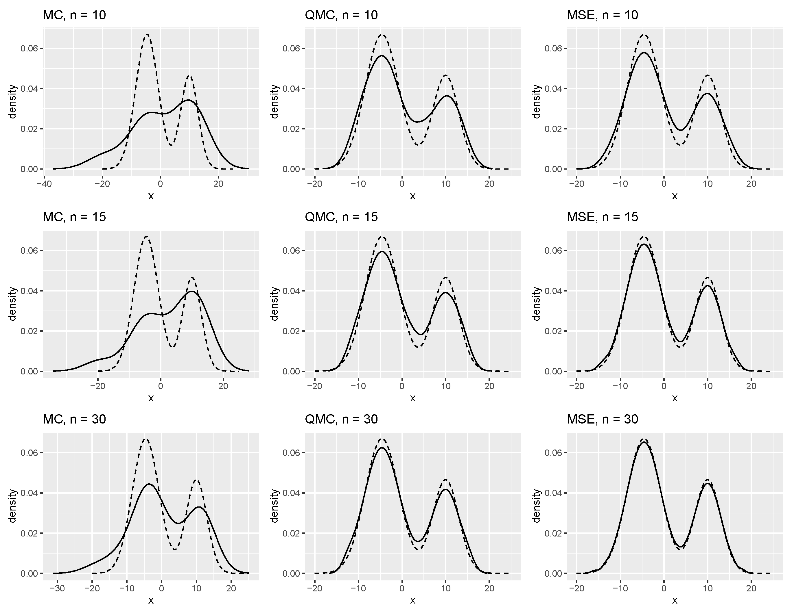
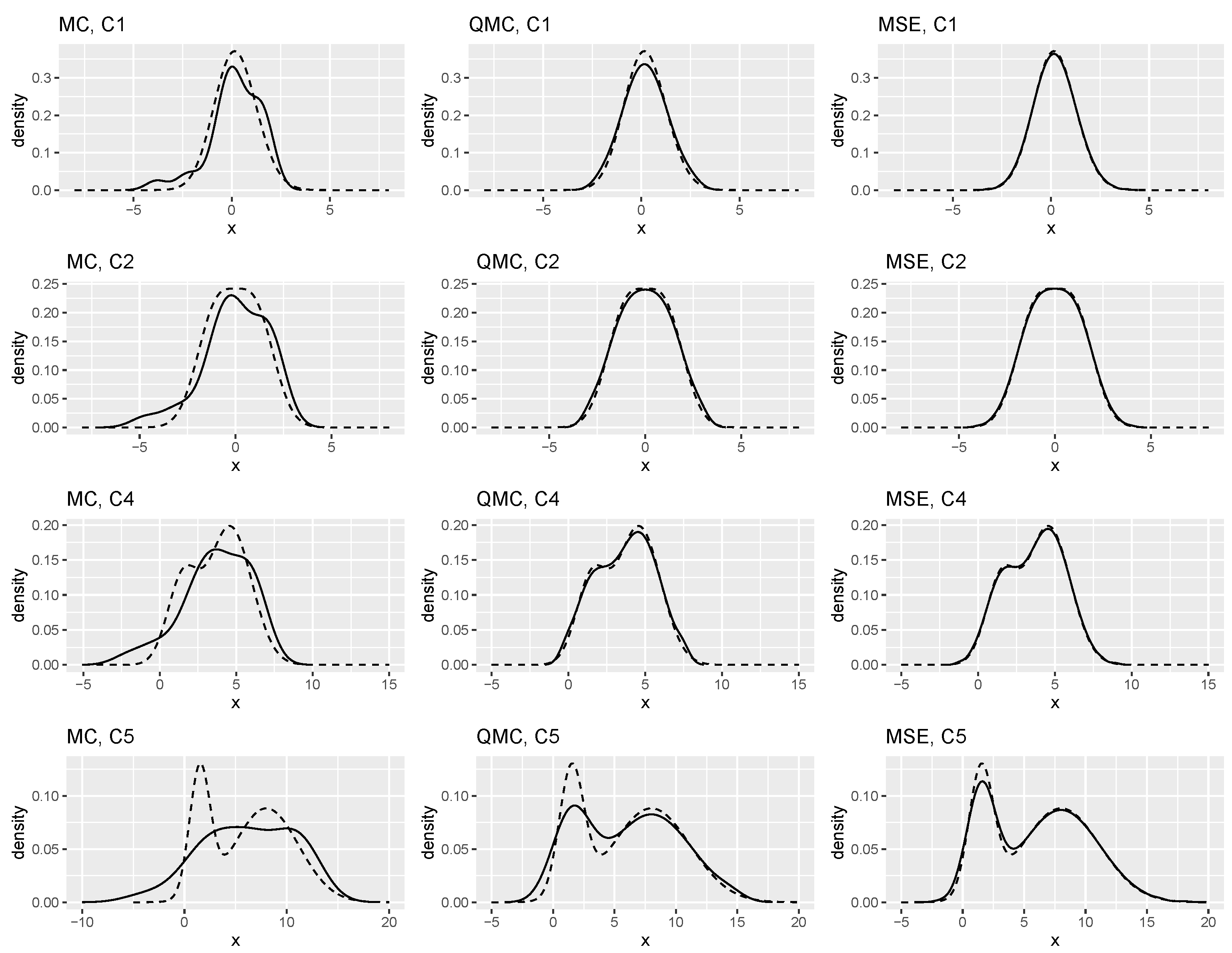
5.2. Kernel Density Estimations
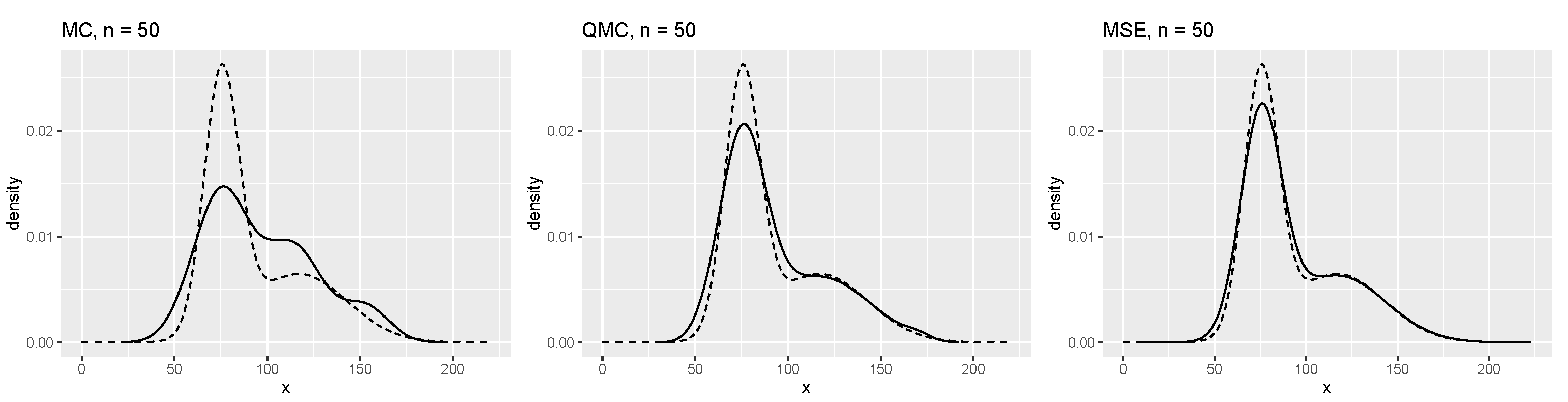
5.3. Real Data Example
6. Discussion
Author Contributions
Funding
Institutional Review Board Statement
Informed Consent Statement
Data Availability Statement
Conflicts of Interest
Appendix A
References
- Andrew, G.; Qi, C.; Alan, D.K.; Ron, W. Pulse pileup rejection methods using a two-component Gaussian Mixture Model for fast neutron detection with pulse shape discriminating scintillator. Nucl. Instrum. Methods Phys. Res. A Accel. Spectrom. Detect. Assoc. Equip. 2021, 988, 164905. [Google Scholar]
- Kong, L.; Chatzinotas, S.; Öttersten, B. Unified framework for secrecy characteristics with mixture of Gaussian (MoG) distribution. IEEE Wirel. Commun. 2020, 10, 1625–1628. [Google Scholar] [CrossRef]
- Shen, X.; Zhang, Y.; Sata, K.; Shen, T. Gaussian mixture model clustering-based knock threshold learning in automotive engines. IEEE ASME Trans. Mechatron 2020, 6, 2981–2991. [Google Scholar] [CrossRef]
- Mazzeo, D.; Oliveti, G.; Labonia, E. Estimation of wind speed probability density function using a mixture of two truncated normal distributions. Renew. Energy 2018, 115, 1260–1280. [Google Scholar] [CrossRef]
- Ouarda, T.B.M.J.; Charron, C. On the mixture of wind speed distribution in a Nordic region. Energy Convers. Manag. 2018, 174, 33–44. [Google Scholar] [CrossRef]
- Venkataraman, S. Value at risk for a mixture of normal distributions: The use of quasi- Bayesian estimation techniques. Econ. Perspect. Fed. Reserve Bank Chic. 1997, 21, 2–13. [Google Scholar]
- Duan, R.; Ning, Y.; Wang, S.; Lindsay, B.G.; Carroll, R.J.; Chen, Y. A fast score test for generalized mixture models. Biometrics 2020, 76, 811–820. [Google Scholar] [CrossRef]
- Di, C.Z.; Liang, K.Y. Likelihood ratio resting for admixture models with application to genetic linkage analysis. Biometrics 2011, 67, 1249–1259. [Google Scholar] [CrossRef]
- Hartigan, J.A. A failure of likelihood asymptotics for normal mixtures. In Proceedings of the Berkeley Conference in Honor of Jerzy Neyman and Jack Kiefer; Wadsworth: Belmont, CA, USA, 1985; Volume 2, pp. 807–810. [Google Scholar]
- Day, N.E. Estimating the components of a mixture of normal distributions. Biometrika 1969, 56, 463–474. [Google Scholar] [CrossRef]
- Panić, B.; Klemenc, J.; Nagode, M. Improved Initialization of the EM Algorithm for Mixture Model Parameter Estimation. Mathematics 2020, 8, 373. [Google Scholar] [CrossRef] [Green Version]
- Li, Y.; Fang, K.T. A new approach to parameter estimation of mixture of two normal distributions. Commun. Stat. Simul. Comput. 2022, 1–27. [Google Scholar] [CrossRef]
- Chen, J. Consistency of the mle under mixture models. Stat. Sci. 2017, 32, 47–63. [Google Scholar] [CrossRef]
- Wu, X. Optimal quantization by matrix searching. J. Algorithms 1991, 12, 663–673. [Google Scholar] [CrossRef]
- Graf, S.; Luschgy, H. Foundations of Quantization for Probability Distributions; Springer-Verlag: Berlin/Heidelberg, Germany, 2007. [Google Scholar]
- Gersho, A.; Gray, R.M. Vector Quantization and Signal Compression; Kluwer: Boston, MA, USA, 1992. [Google Scholar]
- Max, J. Quantizing for minimum distortion. IEEE Trans. Inf. Theory 1960, 6, 7–12. [Google Scholar] [CrossRef]
- Flury, B. Principal points. Biometrika 1990, 77, 33–41. [Google Scholar] [CrossRef]
- Trushkin, A. Sufficient conditions for uniqueness of a locally optimal quantizer for a class of convex error weighting functions. IEEE Trans. Inf. Theory 1982, 28, 187–198. [Google Scholar] [CrossRef]
- Tarpey, T. Two principal points of symmetric, strongly unimodal distributions. Stat. Probab. Lett. 1994, 20, 253–257. [Google Scholar] [CrossRef]
- Yamamoto, W.; Shinozaki, N. On uniqueness of two principal points for univariate location mixtures. Stat. Probab. 2000, 46, 33–42. [Google Scholar] [CrossRef]
- Lloyd, S.P. Least squares quantization in PCM. IEEE Trans. Inform. 1982, 28, 129–137. [Google Scholar] [CrossRef] [Green Version]
- Kieffer, J. Exponential rate of convergence for Lloyd’s method. IEEE Trans. Inform. Theory 1982, 28, 205–210. [Google Scholar] [CrossRef]
- Rowe, S. An algorithm for computing principal points with respect to a loss function in the unidimensional case. Stat. Comput. 1996, 6, 187–190. [Google Scholar] [CrossRef]
- Chakraborty, S.; Roychowdhury, M.K.; Sifuentes, J. High precision numerical computation of principal points for univariate distributions. Sankhya B 2021, 83, 558–584. [Google Scholar] [CrossRef]
- Fang, K.T.; He, S.D. The Problem of Selecting a Given Number of Representative Points in a Normal Population and a Generalized Mills’ Ratio; Technical Report SOLONR327; Department of Statistics, Stanford University: Stanford, CA, USA, 1964. [Google Scholar]
- Zhou, M.; Wang, W. Representative points of Student’s tn distribution and their applications in statistical simulation. Acta Math. Appl. Sin. 2016, 39, 620–640. [Google Scholar]
- Fu, H. The problem of selecting a specified number of representative points from a Gamma population. J. China Univ. Min. Technol. 1985, 4, 107–117. [Google Scholar]
- Wang, H. Problems of choosing representative points of given data in S-type distributions. J. Fuzhou Univ. 1995, 23, 7–13. [Google Scholar]
- Fu, H. The problem of selecting a specified number of representative points from a Weibull population. J. Wuxi Inst. Light Ind. 1993, 22, 78–83. [Google Scholar]
- Fei, R. The problem of selecting representative points from Pearson distributions population. J. Wuxi Inst. Light Ind. 1990, 9, 71–78. [Google Scholar]
- Fang, K.T.; He, P.; Yang, J. Set of representative points of statistical distributions and their applications. Sci. Sin. Math 2020, 50, 1149–1168. [Google Scholar]
- Eisenberger, I. Genesis of bimodal distributions. Technometrics 1964, 6, 357–363. [Google Scholar] [CrossRef]
- Behboodian, J. On the modes of a mixture of two normal distributions. Technometrics 1970, 12, 131–139. [Google Scholar] [CrossRef]
- Aitkin, M.; Wilson, G.T. Mixture models, outliers, and the em algorithm. Technometrics 1980, 22, 325–331. [Google Scholar] [CrossRef]
- Fei, R. Statistical relationship between the representative point and the population. J. Wuxi Inst. Light Ind. 1991, 10, 78–81. [Google Scholar]
- Flury, B. Estimation of principal points. J. R. Stat. Soc. C Appl. Stat. 1993, 42, 139–151. [Google Scholar] [CrossRef]
- Li, L.; Flury, B. Uniqueness of principal points for univariate distributions. Stat. Probab. Lett. 1995, 25, 323–327. [Google Scholar] [CrossRef]
- Bagnoli, M.; Bergstrom, T. Log-concave probability and its applications. Econ. Theory 2005, 26, 445–469. [Google Scholar] [CrossRef] [Green Version]
- Saumard, A.; Wellner, J.A. Log-concavity and strong log-concavity: A review. Stat. Surv. 2014, 8, 45–114. [Google Scholar] [CrossRef] [PubMed]
- Fang, K.T.; Wang, Y. Number-Theoretic Methods in Statistics, 1st ed.; Chapman and Hall: London, UK, 1994. [Google Scholar]
- Fang, K.T.; Wang, Y.; Bentler, P.M. Some applications of number-theoretic methods in statistics. Stat. Sci. 1994, 9, 416–428. [Google Scholar] [CrossRef]
- Parzen, E. On estimation of a probability density function and mode. Ann. Math. Statist. 1962, 33, 1065–1076. [Google Scholar] [CrossRef]
- Rosenblatt, M. Remarks on some nonparametric estimates of a density function. Ann. Math. Statist. 1956, 27, 832–837. [Google Scholar] [CrossRef]
- Wolberg, W.; Street, W.; Mangasarian, O. Breast Cancer Wisconsin (Diagnostic). UCI Mach. Learn. Repos. 1995. Available online: https://archive.ics.uci.edu/ml/datasets/Breast+Cancer+Wisconsin+%28Diagnostic%29 (accessed on 28 August 2022).


| Size | IG(%) | n = 1 | n = 2 | n = 3 | n = 4 | n = 5 | n = 6 | n = 7 | n = 8 | n = 9 | n = 10 | n = 11 | n = 12 | n = 13 | n = 14 | n = 15 |
|---|---|---|---|---|---|---|---|---|---|---|---|---|---|---|---|---|
| n = 1 | 0 | 6.05 | ||||||||||||||
| n = 2 | 73.96867346 | 2.423613543 | 9.348758993 | |||||||||||||
| n = 3 | 88.05491179 | 1.791094154 | 6.958435648 | 11.2740348 | ||||||||||||
| n = 4 | 92.63599987 | 1.578947831 | 5.686264735 | 8.875275128 | 12.41300952 | |||||||||||
| n = 5 | 94.8041442 | 1.359320939 | 4.411547025 | 7.247043817 | 9.887325817 | 13.08347976 | ||||||||||
| n = 6 | 96.27601491 | 0.874142484 | 2.777767093 | 5.689605266 | 8.07288434 | 10.47036442 | 13.48934091 | |||||||||
| n = 7 | 97.19355685 | 0.721547318 | 2.432989485 | 4.978270697 | 7.092697743 | 9.077360483 | 11.21789261 | 14.02854444 | ||||||||
| n = 8 | 97.78091815 | 0.590565454 | 2.169171019 | 4.283239715 | 6.255118286 | 8.021071278 | 9.789159766 | 11.76997495 | 14.43927428 | |||||||
| n = 9 | 98.20500143 | 0.380162232 | 1.790678064 | 3.347424327 | 5.318647716 | 7.004963804 | 8.600761793 | 10.24988317 | 12.13627649 | 14.71782742 | ||||||
| n = 10 | 98.52422536 | 0.239819589 | 1.562145486 | 2.880667144 | 4.710947518 | 6.30573222 | 7.767300571 | 9.212233319 | 10.74770084 | 12.53926685 | 15.02845211 | |||||
| n = 11 | 98.76043213 | 0.133566173 | 1.399444615 | 2.585563018 | 4.193896755 | 5.719336628 | 7.08614538 | 8.397705465 | 9.732586337 | 11.18033667 | 12.8953116 | 15.30709701 | ||||
| n = 12 | 98.94303836 | 0.008599829 | 1.218033572 | 2.284440454 | 3.615134473 | 5.110029435 | 6.427649977 | 7.659566762 | 8.874284538 | 10.13383388 | 11.51870386 | 13.17678786 | 15.52993185 | |||
| n = 13 | 99.08923755 | −0.108377781 | 1.056999406 | 2.036526303 | 3.161785634 | 4.587501185 | 5.867069117 | 7.039498911 | 8.169244053 | 9.306265285 | 10.50274013 | 11.83310719 | 13.44080446 | 15.74095873 | ||
| n = 14 | 99.20635891 | −0.203011483 | 0.932442594 | 1.855030921 | 2.855603653 | 4.153620796 | 5.396210451 | 6.519930545 | 7.584211116 | 8.6328177 | 9.705262108 | 10.84759276 | 12.13029145 | 13.69267353 | 15.94396209 | |
| n = 15 | 99.30172785 | −0.29980057 | 0.810063673 | 1.684262651 | 2.586658213 | 3.723095049 | 4.937162824 | 6.029382725 | 7.04819063 | 8.034822997 | 9.0224751 | 10.04458986 | 11.14397262 | 12.38790997 | 13.9129648 | 16.12264763 |
| n = 16 | 99.38099587 | −0.397412309 | 0.691626392 | 1.525271182 | 2.350810489 | 3.338672949 | 4.506794964 | 5.5768593 | 6.562313213 | 7.503042441 | 8.429158158 | 9.367664013 | 10.34815779 | 11.41056413 | 12.62052747 | 14.11295278 |
| n = 17 | 99.44737405 | −0.485192498 | 0.589176996 | 1.392128437 | 2.162551368 | 3.042665875 | 4.129813389 | 5.177772808 | 6.13525477 | 7.038712328 | 7.91663556 | 8.792274267 | 9.688605761 | 10.63278608 | 11.66254558 | 12.84233566 |
| n = 18 | 99.50344049 | −0.571828837 | 0.491812217 | 1.269172171 | 1.995295568 | 2.791623221 | 3.773842904 | 4.799051507 | 5.736150584 | 6.611428786 | 7.452441414 | 8.28057358 | 9.115139619 | 9.97629137 | 10.88945494 | 11.89121853 |
| n = 19 | 99.55136666 | −0.66008555 | 0.396525787 | 1.152105407 | 1.841299097 | 2.57076108 | 3.446966179 | 4.437820157 | 5.359804761 | 6.213672075 | 7.026204885 | 7.817675083 | 8.605241459 | 9.405393281 | 10.23665219 | 11.1229878 |
| n = 20 | 99.59264581 | −0.744557874 | 0.308685016 | 1.046738329 | 1.706464312 | 2.38502281 | 3.173673557 | 4.108561179 | 5.015150185 | 5.851445576 | 6.640528149 | 7.402097575 | 8.152222797 | 8.905109605 | 9.6754321 | 10.48030964 |
| n = 21 | 99.62688834 | −0.807393885 | 0.245705351 | 0.972803654 | 1.614016128 | 2.261506603 | 2.995836819 | 3.877267405 | 4.771000758 | 5.596662068 | 6.371402271 | 7.114885147 | 7.842354992 | 8.56690891 | 9.301567899 | 10.06021893 |
| n = 22 | 99.65267792 | −0.870229896 | 0.18467363 | 0.902417461 | 1.527423029 | 2.148251749 | 2.836712777 | 3.661464882 | 4.538754269 | 5.355747462 | 6.119001391 | 6.847298881 | 7.555595105 | 8.2564044 | 8.961304462 | 9.682558988 |
| n = 23 | 99.68714839 | −1.00264325 | 0.061578323 | 0.763675619 | 1.360571692 | 1.93647453 | 2.549550382 | 3.262541556 | 4.082228812 | 4.882146188 | 5.62653707 | 6.329686539 | 7.006023507 | 7.667600776 | 8.324251635 | 8.985487835 |
| n = 24 | 99.71006407 | −1.065479261 | 0.006070463 | 0.702703328 | 1.288991946 | 1.84784457 | 2.433452432 | 3.102572966 | 3.884230722 | 4.674021592 | 5.411091343 | 6.104787035 | 6.769153696 | 7.415835925 | 8.054367628 | 8.693504163 |
| n = 25 | 99.72667915 | −1.128315272 | −0.047690507 | 0.644552282 | 1.221535747 | 1.765644791 | 2.327686503 | 2.959453199 | 3.700582468 | 4.477186241 | 5.208030648 | 5.893640702 | 6.547658551 | 7.181513639 | 7.804599568 | 8.425070077 |
| n = 26 | 99.75125918 | −1.253987293 | −0.15014384 | 0.536126724 | 1.097771571 | 1.617523743 | 2.141690864 | 2.712750935 | 3.374707329 | 4.113054579 | 4.83194039 | 5.5054193 | 6.143465574 | 6.75717493 | 7.355574511 | 7.946356234 |
| n = 27 | 99.7644673 | −1.316823304 | −0.198892331 | 0.485716419 | 1.04132981 | 1.551252832 | 2.060371533 | 2.607712131 | 3.23559288 | 3.948775949 | 4.660267019 | 5.328921948 | 5.960757926 | 6.566486661 | 7.154979624 | 7.733845897 |
| n = 28 | 99.78349091 | −1.442495326 | −0.292262094 | 0.390813208 | 0.93628443 | 1.42946724 | 1.913078033 | 2.420923189 | 2.990243483 | 3.646175602 | 4.337656222 | 4.997598338 | 5.619209446 | 6.211748648 | 6.783925299 | 7.343011187 |
| n = 29 | 99.79899701 | −1.576585624 | −0.386434972 | 0.297203347 | 0.834313039 | 1.313203717 | 1.775255231 | 2.250702302 | 2.770884396 | 3.366307402 | 4.024390942 | 4.673732574 | 5.286833944 | 5.868286401 | 6.426797921 | 6.969342579 |
| n = 30 | 99.81170752 | −1.682670291 | −0.457277753 | 0.228182859 | 0.760148622 | 1.22985285 | 1.678073187 | 2.1331801 | 2.622495132 | 3.176383558 | 3.800806147 | 4.43873492 | 5.046032586 | 5.620844886 | 6.170757585 | 6.702586356 |
| Size | IG(%) | n=16 | n=17 | n=18 | n=19 | n=20 | n=21 | n=22 | n=23 | n=24 | n=25 | n=26 | n=27 | n=28 | n=29 | n=30 |
| n = 16 | 16.28634947 | |||||||||||||||
| n = 17 | 14.30367481 | 16.44282304 | ||||||||||||||
| n = 18 | 13.04446388 | 14.4792947 | 16.58833697 | |||||||||||||
| n = 19 | 12.10037508 | 13.2300635 | 14.64126979 | 16.7219755 | ||||||||||||
| n = 20 | 11.34285496 | 12.29780724 | 13.40525617 | 14.79379596 | 16.84910295 | |||||||||||
| n = 21 | 10.8607438 | 11.72780172 | 12.70058597 | 13.84935175 | 15.33707755 | 17.28340665 | ||||||||||
| n = 22 | 10.4339771 | 11.23436194 | 12.11083106 | 13.10798308 | 14.31132602 | 15.93482661 | 17.34624266 | |||||||||
| n = 23 | 9.661538521 | 10.36362581 | 11.10688902 | 11.91274135 | 12.81312891 | 13.86725272 | 15.20051003 | 17.19050787 | ||||||||
| n = 24 | 9.342118103 | 10.01037951 | 10.71000566 | 11.45689056 | 12.27427554 | 13.19971393 | 14.30402627 | 15.7507717 | 17.54149202 | |||||||
| n = 25 | 9.051060731 | 9.69077992 | 10.3544829 | 11.05458254 | 11.80913245 | 12.64330719 | 13.60228946 | 14.77474311 | 16.38044961 | 17.60432804 | ||||||
| n = 26 | 8.536378676 | 9.132715108 | 9.742633602 | 10.37472033 | 11.04041181 | 11.75447389 | 12.53836963 | 13.42875426 | 14.49230883 | 15.88156445 | 17.55395655 | |||||
| n = 27 | 8.309644238 | 8.888833378 | 9.478009352 | 10.08458152 | 10.71813121 | 11.3899024 | 12.11712718 | 12.92564178 | 13.85914468 | 15.00363721 | 16.57893718 | 17.79283607 | ||||
| n = 28 | 7.895239264 | 8.446310291 | 9.001792295 | 9.567957905 | 10.1508894 | 10.75969929 | 11.40496423 | 12.10040839 | 12.86983695 | 13.75034321 | 14.81094566 | 16.21633053 | 17.74246458 | |||
| n = 29 | 7.501685726 | 8.029355922 | 8.557203492 | 9.090117312 | 9.633724516 | 10.19370059 | 10.77724624 | 11.39451777 | 12.05901994 | 12.78828981 | 13.61421997 | 14.59337111 | 15.8468082 | 17.73883763 | ||
| n = 30 | 7.222328932 | 7.735220638 | 8.245656964 | 8.758184601 | 9.277234144 | 9.808036926 | 10.35632242 | 10.92893176 | 11.535665 | 12.1903433 | 12.91039171 | 13.7267179 | 14.69620142 | 15.938859 | 17.81798303 |
| Size | n = 1 | n = 2 | n = 3 | n = 4 | n = 5 | n = 6 | n = 7 | n = 8 | n = 9 | n = 10 | n = 11 | n = 12 | n = 13 | n = 14 | n = 15 |
|---|---|---|---|---|---|---|---|---|---|---|---|---|---|---|---|
| n = 1 | 1 | ||||||||||||||
| n = 2 | 0.476345265 | 0.523654735 | |||||||||||||
| n = 3 | 0.387464318 | 0.359100239 | 0.253435443 | ||||||||||||
| n = 4 | 0.353593647 | 0.233434993 | 0.271896131 | 0.141075228 | |||||||||||
| n = 5 | 0.312139375 | 0.160211605 | 0.227469427 | 0.205544828 | 0.094634765 | ||||||||||
| n = 6 | 0.206142213 | 0.174695598 | 0.172388178 | 0.20611581 | 0.1677893 | 0.0728689 | |||||||||
| n = 7 | 0.17402589 | 0.182924593 | 0.130105109 | 0.170452309 | 0.168524295 | 0.123657199 | 0.050310606 | ||||||||
| n = 8 | 0.148364963 | 0.184887644 | 0.102463575 | 0.139101297 | 0.154034462 | 0.138352315 | 0.095527568 | 0.037268176 | |||||||
| n = 9 | 0.111839247 | 0.175468356 | 0.098175866 | 0.110882403 | 0.136236259 | 0.139132192 | 0.118848093 | 0.079272555 | 0.030145028 | ||||||
| n = 10 | 0.091047449 | 0.162027494 | 0.107962981 | 0.089711281 | 0.115464291 | 0.126865145 | 0.120988109 | 0.098694819 | 0.063649047 | 0.023589383 | |||||
| n = 11 | 0.077249903 | 0.149507214 | 0.115127365 | 0.075580739 | 0.097256732 | 0.112512798 | 0.115078771 | 0.104639772 | 0.082469925 | 0.051786667 | 0.018790114 | ||||
| n = 12 | 0.06311153 | 0.133495811 | 0.119914378 | 0.070361904 | 0.081276208 | 0.098651851 | 0.106732365 | 0.104436071 | 0.09200911 | 0.070801066 | 0.043625389 | 0.015584317 | |||
| n = 13 | 0.051819253 | 0.118223832 | 0.119878686 | 0.074659113 | 0.068597117 | 0.085488051 | 0.096487045 | 0.099411465 | 0.093983698 | 0.080694416 | 0.06086164 | 0.036896332 | 0.012999352 | ||
| n = 14 | 0.043956182 | 0.106194926 | 0.116981805 | 0.080419452 | 0.060017208 | 0.073892167 | 0.086064206 | 0.092054959 | 0.091352386 | 0.084004277 | 0.070598114 | 0.052327967 | 0.031260696 | 0.010875655 | |
| n = 15 | 0.036991832 | 0.094522794 | 0.111997602 | 0.085713267 | 0.056120593 | 0.063784217 | 0.07627941 | 0.084242426 | 0.086815907 | 0.083831215 | 0.075501554 | 0.062405967 | 0.045612056 | 0.026915914 | 0.009265246 |
| n = 16 | 0.030970785 | 0.08359798 | 0.105561628 | 0.089129393 | 0.057476898 | 0.055547814 | 0.067262533 | 0.076343083 | 0.081116235 | 0.081277246 | 0.076817424 | 0.068008853 | 0.055438445 | 0.040065225 | 0.023405491 |
| n = 17 | 0.026329752 | 0.074577724 | 0.099046204 | 0.090265596 | 0.061212707 | 0.049819795 | 0.059270497 | 0.068725831 | 0.07483451 | 0.077153565 | 0.075560653 | 0.070150495 | 0.061208778 | 0.049295436 | 0.035243746 |
| n = 18 | 0.022388871 | 0.066477408 | 0.092329138 | 0.089744645 | 0.065383529 | 0.046969307 | 0.052327092 | 0.061641025 | 0.068566526 | 0.072387282 | 0.072915943 | 0.070124071 | 0.064152989 | 0.05530825 | 0.04408941 |
| n = 19 | 0.018954148 | 0.05906334 | 0.085494176 | 0.087881986 | 0.068975212 | 0.047249092 | 0.046643591 | 0.055133522 | 0.062493136 | 0.067346577 | 0.069425059 | 0.068645952 | 0.065044622 | 0.058785066 | 0.050171849 |
| n = 20 | 0.016148251 | 0.05269626 | 0.079099701 | 0.085167118 | 0.071336031 | 0.049540776 | 0.042608453 | 0.049336144 | 0.056760187 | 0.062239745 | 0.065404713 | 0.066132161 | 0.064389253 | 0.060245283 | 0.053877025 |
| n = 21 | 0.014331958 | 0.048430958 | 0.074565544 | 0.082767546 | 0.072337221 | 0.05179405 | 0.040835527 | 0.045512277 | 0.052752376 | 0.058534445 | 0.062303139 | 0.063893207 | 0.063259337 | 0.060417543 | 0.055480215 |
| n = 22 | 0.012721458 | 0.044540251 | 0.070242658 | 0.08013962 | 0.072760187 | 0.054104658 | 0.040211832 | 0.042221455 | 0.049059046 | 0.055010951 | 0.059210555 | 0.061477411 | 0.061736997 | 0.059989253 | 0.05627992 |
| n = 23 | 0.00990561 | 0.03737658 | 0.061822934 | 0.074211324 | 0.072097587 | 0.058151382 | 0.041863221 | 0.037225831 | 0.042159573 | 0.048087511 | 0.052845873 | 0.056113322 | 0.057779445 | 0.057780153 | 0.056134082 |
| n = 24 | 0.008805846 | 0.034455817 | 0.058232304 | 0.07137654 | 0.071229446 | 0.059487707 | 0.043422501 | 0.035940772 | 0.039375256 | 0.045084501 | 0.049979047 | 0.053555599 | 0.055688975 | 0.056310847 | 0.055408925 |
| n = 25 | 0.007835227 | 0.031801335 | 0.054879126 | 0.068590254 | 0.070114173 | 0.060461631 | 0.045137918 | 0.035392009 | 0.03698507 | 0.0423196 | 0.047261938 | 0.051067098 | 0.053577742 | 0.054715607 | 0.054452555 |
| n = 26 | 0.006224218 | 0.027205375 | 0.048850998 | 0.063229792 | 0.067380876 | 0.061343996 | 0.048329267 | 0.036125954 | 0.033490464 | 0.037494457 | 0.042337381 | 0.046421368 | 0.049455062 | 0.05135021 | 0.052054826 |
| n = 27 | 0.005558847 | 0.025219572 | 0.046180942 | 0.060732959 | 0.065893864 | 0.061385524 | 0.049660122 | 0.037078651 | 0.032429443 | 0.035458909 | 0.0401411 | 0.044290323 | 0.047496275 | 0.049661125 | 0.05073257 |
| n = 28 | 0.004453538 | 0.021751247 | 0.041353249 | 0.056001064 | 0.062714317 | 0.060793876 | 0.051663756 | 0.03947053 | 0.03163836 | 0.03212298 | 0.036155425 | 0.040303073 | 0.043747931 | 0.046319341 | 0.047957622 |
| n = 29 | 0.00354088 | 0.018663736 | 0.036880282 | 0.051383805 | 0.059243655 | 0.059503741 | 0.052872241 | 0.04201032 | 0.032382329 | 0.029760912 | 0.032550275 | 0.036479152 | 0.040032496 | 0.042890716 | 0.044945877 |
| n = 30 | 0.002970755 | 0.016592742 | 0.033778207 | 0.04805665 | 0.056550782 | 0.058180936 | 0.053260427 | 0.043721964 | 0.033665097 | 0.028835929 | 0.030238379 | 0.033812616 | 0.037361267 | 0.040340641 | 0.042626351 |
| Size | n=16 | n=17 | n=18 | n=19 | n=20 | n=21 | n=22 | n=23 | n=24 | n=25 | n=26 | n=27 | n=28 | n=29 | n=30 |
| n = 16 | 0.007980967 | ||||||||||||||
| n = 17 | 0.020402411 | 0.0069023 | |||||||||||||
| n = 18 | 0.031238477 | 0.017935945 | 0.006020091 | ||||||||||||
| n = 19 | 0.039643705 | 0.027868553 | 0.015883139 | 0.005297276 | |||||||||||
| n = 20 | 0.045564607 | 0.035709574 | 0.024931537 | 0.014128309 | 0.00468487 | ||||||||||
| n = 21 | 0.048648071 | 0.040209581 | 0.030572419 | 0.020378759 | 0.009969009 | 0.003006819 | |||||||||
| n = 22 | 0.050750019 | 0.043622132 | 0.035190543 | 0.025884626 | 0.016344924 | 0.006300653 | 0.002200855 | ||||||||
| n = 23 | 0.052872361 | 0.048102178 | 0.042006149 | 0.0347745 | 0.026744056 | 0.018362538 | 0.0102406 | 0.00334319 | |||||||
| n = 24 | 0.053025196 | 0.049212753 | 0.044074126 | 0.037789391 | 0.030594504 | 0.022825265 | 0.014931638 | 0.007004033 | 0.002189011 | ||||||
| n = 25 | 0.052785998 | 0.049773524 | 0.04550369 | 0.040111187 | 0.033742595 | 0.026657665 | 0.019211571 | 0.011825 | 0.004236389 | 0.001561098 | |||||
| n = 26 | 0.051557543 | 0.049867076 | 0.047016612 | 0.04310501 | 0.038228517 | 0.032505294 | 0.02616132 | 0.019458127 | 0.012740819 | 0.006022389 | 0.002043046 | ||||
| n = 27 | 0.050683184 | 0.049514808 | 0.047249249 | 0.043962351 | 0.039712734 | 0.034622285 | 0.028862251 | 0.022619073 | 0.016162828 | 0.009879687 | 0.003525194 | 0.001286131 | |||
| n = 28 | 0.048627358 | 0.048312446 | 0.047034448 | 0.0447928 | 0.041663535 | 0.037728136 | 0.033023665 | 0.027736878 | 0.02204455 | 0.016132384 | 0.010332258 | 0.004543942 | 0.001581292 | ||
| n = 29 | 0.046171777 | 0.046550019 | 0.046060452 | 0.044731083 | 0.042572485 | 0.03961438 | 0.035958816 | 0.031692546 | 0.026860541 | 0.021641685 | 0.016251299 | 0.010907742 | 0.005947253 | 0.001899505 | |
| n = 30 | 0.044185774 | 0.04497709 | 0.044983309 | 0.044206637 | 0.042668036 | 0.040397221 | 0.037419586 | 0.033819188 | 0.029698301 | 0.025094318 | 0.020149648 | 0.015081924 | 0.010092536 | 0.005486728 | 0.00174696 |
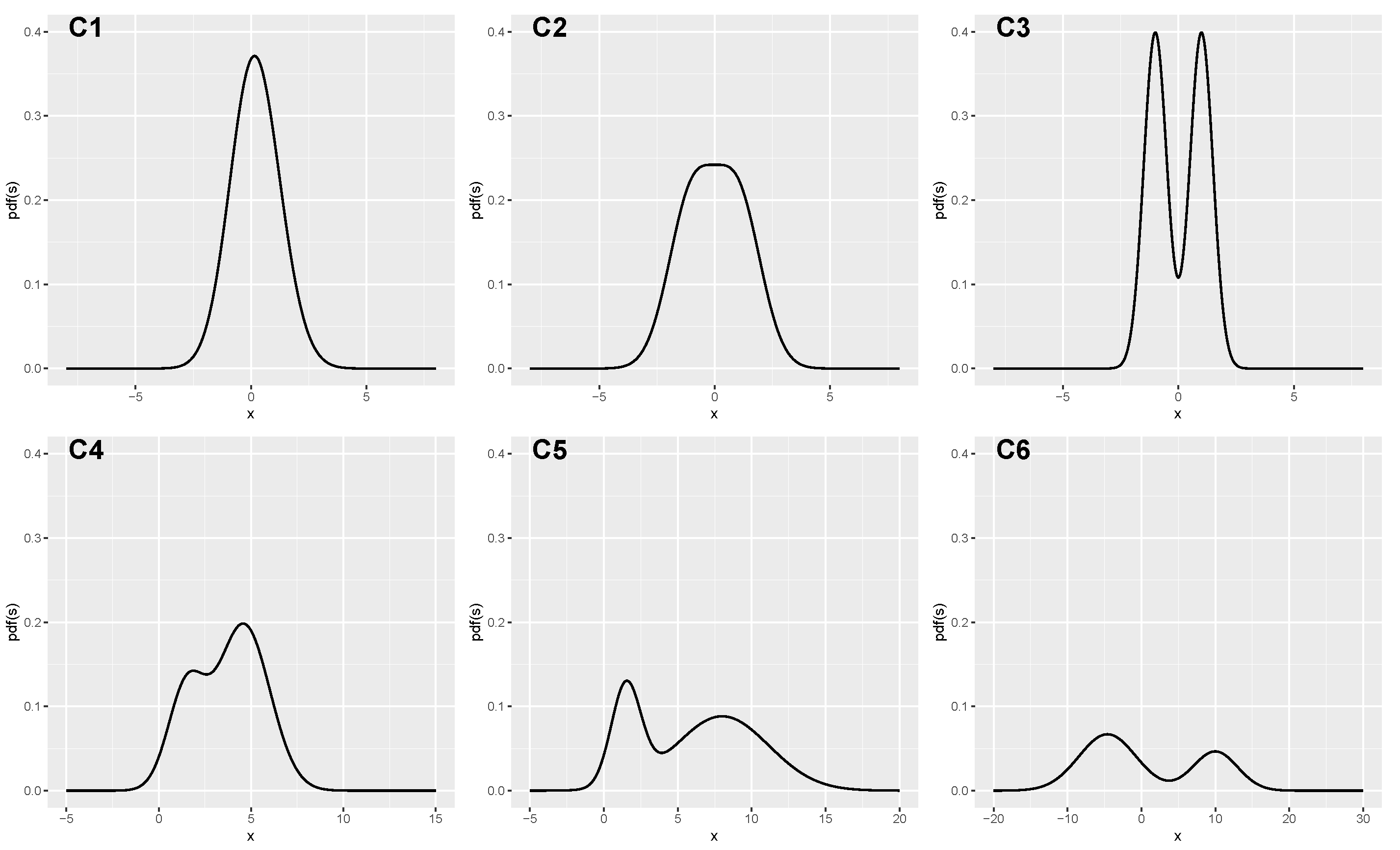
| Distribution | E(X) | Var(X) | |||||
|---|---|---|---|---|---|---|---|
| C1 | 0.80 | 0.0 | 1.00 | 1.0 | 1.00 | 0.20 | 1.16 |
| C2 | 0.50 | 1.0 | 1.00 | −1.0 | 1.00 | 0.00 | 2.00 |
| C3 | 0.50 | 1.0 | 0.25 | −1.0 | 0.25 | 0.00 | 1.25 |
| C4 | 0.70 | 4.6 | 2.00 | 1.5 | 1.00 | 3.67 | 3.72 |
| C5 | 0.70 | 8.0 | 10.00 | 1.5 | 1.00 | 6.05 | 16.17 |
| C6 | 0.65 | −4.6 | 15.00 | 10.0 | 9.00 | 0.51 | 61.39 |
| Size | Fang-He | k-Means | Fang-He | k-Means |
|---|---|---|---|---|
| C1 | C2 | |||
| 2 | 0.00000 | 0.00240 | 0.00000 | 0.00334 |
| 3 | 0.00000 | 0.00215 | 0.00000 | 0.00217 |
| 4 | 0.00000 | 0.00158 | 0.00000 | 0.00198 |
| 5 | 0.00000 | 0.00142 | 0.00000 | 0.00180 |
| 10 | 0.00000 | 0.00054 | 0.00000 | 0.00064 |
| 15 | 0.00000 | 0.00037 | 0.00000 | 0.00052 |
| 30 | 0.00000 | 0.00020 | 0.00000 | 0.00023 |
| C3 | C4 | |||
| 2 | 0.00000 | 0.00184 | 0.00000 | 0.00223 |
| 3 | 0.00000 | 0.00113 | 0.00000 | 0.00255 |
| 4 | 0.00000 | 0.00152 | 0.00000 | 0.00292 |
| 5 | 0.00000 | 0.00093 | 0.00000 | 0.00259 |
| 10 | 0.00000 | 0.00053 | 0.00000 | 0.00111 |
| 15 | 0.00000 | 0.00030 | 0.00000 | 0.00072 |
| 30 | 0.00000 | 0.00013 | 0.00000 | 0.00036 |
| C5 | C6 | |||
| 2 | 0.00000 | 0.00511 | 0.00000 | 0.01290 |
| 3 | 0.00000 | 0.00674 | 0.00000 | 0.00797 |
| 4 | 0.00000 | 0.00490 | 0.00000 | 0.00742 |
| 5 | 0.00000 | 0.00383 | 0.00000 | 0.00764 |
| 10 | 0.00000 | 0.00146 | 0.00000 | 0.00309 |
| 15 | 0.00000 | 0.00102 | 0.00000 | 0.00206 |
| 30 | 0.00000 | 0.00072 | 0.00000 | 0.00096 |
| Size | Fang-He | k-Means | Fang-He | k-Means |
|---|---|---|---|---|
| C1 | C2 | |||
| 2 | 63.6508 | 63.6483 | 68.0514 | 68.0489 |
| 3 | 80.9919 | 80.9881 | 83.4876 | 83.4856 |
| 4 | 88.2662 | 88.2637 | 89.9059 | 89.9039 |
| 5 | 92.0203 | 92.0189 | 93.1672 | 93.1661 |
| 10 | 97.7140 | 97.7132 | 98.0585 | 98.0576 |
| 15 | 98.9306 | 98.9290 | 99.0936 | 99.0892 |
| 30 | 99.7174 | 99.7154 | 99.7608 | 99.7602 |
| C3 | C4 | |||
| 2 | 81.3643 | 81.3636 | 70.0302 | 70.0296 |
| 3 | 88.4198 | 88.4181 | 84.7832 | 84.7818 |
| 4 | 93.5704 | 93.5684 | 90.6243 | 90.6219 |
| 5 | 95.3915 | 95.3903 | 93.6827 | 93.6815 |
| 10 | 98.7165 | 98.7152 | 98.2091 | 98.2072 |
| 15 | 99.3997 | 99.3988 | 99.1646 | 99.1608 |
| 30 | 99.8417 | 99.8410 | 99.7797 | 99.7790 |
| C5 | C6 | |||
| 2 | 73.9687 | 73.9680 | 80.6102 | 80.6094 |
| 3 | 88.0549 | 88.0521 | 89.8819 | 89.8816 |
| 4 | 92.6360 | 92.6350 | 93.2878 | 93.2874 |
| 5 | 94.8041 | 94.8034 | 95.6431 | 95.6424 |
| 10 | 98.5242 | 98.5234 | 98.7264 | 98.7249 |
| 15 | 99.3017 | 99.3007 | 99.4036 | 99.4024 |
| 30 | 99.8117 | 99.8082 | 99.8426 | 99.8418 |
| Size | MC | QMC | MSE |
|---|---|---|---|
| 10 | 0.2937 | 0.1352 | 0.1084 |
| 15 | 0.3033 | 0.0966 | 0.0478 |
| 30 | 0.2082 | 0.0611 | 0.0207 |
| Size | MC | QMC | MSE |
|---|---|---|---|
| 10 | 1.8123 | 0.6206 | 0.4688 |
| 15 | 1.8441 | 0.5819 | 0.3040 |
| 30 | 1.5683 | 0.3890 | 0.2157 |
| Distribution | MC | QMC | MSE |
|---|---|---|---|
| C1 | 0.8201 | 0.3625 | 0.0694 |
| C2 | 0.5901 | 0.1639 | 0.0607 |
| C4 | 0.5237 | 0.1271 | 0.0480 |
| C5 | 0.4474 | 0.2605 | 0.0992 |
| Algorithm | Total Error | MSE |
|---|---|---|
| Fang-He | 0.0000 | 0.5943 |
| k-means | 0.0273 | 1.2921 |
| Method | Mean | Variance | Skewness | Kurtosis |
|---|---|---|---|---|
| Model | 92.9145 | 755.6292 | 0.9853 | 0.2471 |
| MSE (Fang-He) | 92.9145 | 755.0325 | 0.9851 | 0.2392 |
| MSE (k-means) | 92.9091 | 754.2046 | 0.9833 | 0.2066 |
| QMC | 92.8866 | 741.1019 | 0.9538 | 0.0196 |
| MC | 96.9411 | 781.8546 | 0.6179 | −0.6027 |
Publisher’s Note: MDPI stays neutral with regard to jurisdictional claims in published maps and institutional affiliations. |
© 2022 by the authors. Licensee MDPI, Basel, Switzerland. This article is an open access article distributed under the terms and conditions of the Creative Commons Attribution (CC BY) license (https://creativecommons.org/licenses/by/4.0/).
Share and Cite
Li, Y.; Fang, K.-T.; He, P.; Peng, H. Representative Points from a Mixture of Two Normal Distributions. Mathematics 2022, 10, 3952. https://doi.org/10.3390/math10213952
Li Y, Fang K-T, He P, Peng H. Representative Points from a Mixture of Two Normal Distributions. Mathematics. 2022; 10(21):3952. https://doi.org/10.3390/math10213952
Chicago/Turabian StyleLi, Yinan, Kai-Tai Fang, Ping He, and Heng Peng. 2022. "Representative Points from a Mixture of Two Normal Distributions" Mathematics 10, no. 21: 3952. https://doi.org/10.3390/math10213952