
Elaboration of an Algorithm for Solving Hierarchical Inverse Problems in Applied Economics


Faculty of Control Systems, Tomsk State University of Control Systems & Radioelectronics, 40, Lenina Str., 634050 Tomsk, Russia
Mathematics 2022, 10(15), 2779; https://doi.org/10.3390/math10152779
Submission received: 5 July 2022
/
Revised: 3 August 2022
/
Accepted: 3 August 2022
/
Published: 5 August 2022
(This article belongs to the Special Issue Mathematical Methods and Analysis for the Industrial Management and Business, 2nd Edition)
Abstract
:One of the key tools in an organization’s performance management is the goal tree, which is used for solving both direct and inverse problems. This research deals with goal setting based on a model of the future by presenting the goal and subgoal in the form of concrete quantitative and qualitative characteristics and stepwise formation of factors. A stepwise solution to a factor generation problem is considered on the basis of mathematical symmetry. This paper displays an algorithm for solving hierarchical inverse problems with constraints, which is based on recursively traversing the vertices that constitute the separate characteristics. Iterative methods, modified for the case of nonlinear models and the calculation of constraints, were used to generate solutions to the subproblems. To realize the algorithm, the object-oriented architecture, which simplifies the creation and modification of software, was elaborated. Computational experiments with five types of models were conducted, and the solution to a problem related to fast-food restaurant profit generation was reviewed. The metrics of remoteness from set values and t-statistics were calculated for the purpose of testing the received results, and solutions to the subproblems, with the help of a mathematical package using optimization models and a method of inverse calculations, were also provided. The results of computational experiments speak to the compliance of the received results with set constraints and the solution of separate subproblems with the usage of the mathematical package. The cases with the highest solution accuracy reached are specified.
Keywords:
factor tree; hierarchical problem; economic analysis; inverse problem; object-oriented architectureMSC:
68U351. Introduction
The development of an economic system is defined by the effectiveness of the decisions of management specialists who use a range of tools in their activity. One such tool is a goal tree, which is represented by a hierarchical structure that includes the general goal, placed at the root of the tree, and auxiliary subgoals at the first, second, and subsequent levels [1,2]. Maintenance of a company′s financial security [3], development of a “green” economy in the region [4], optimization of the structure of an organization [5], strengthening of its economic position [6], etc., can be considered in the function of a strategic goal. There are various modifications of the goal tree; in particular, the authors of ref. [7] reviewed goal setting based on a model of the future, wherein the goals and subgoals consist of specific quantitative and qualitative factors connected between themselves by functional dependency. The search direction forms the forward or reverse chain, each of which includes a group of subproblems for solving the global task. Thus, when traversing the factor tree from the bottom upward, the calculation of new characteristics based on existing ones using preset functions (direct problem) takes place. Such a principle of traversing allows for carrying out an evaluation and forecasting the goal-oriented characteristic in the case of known data. In the case of traversing the factor tree from the top downward, the values of characteristics, which form the target value, are determined. At the same time, the necessity of analyzing and processing bulk information emerges, which is difficult to perform without relevant mathematical apparatus and software assets. In connection to this, investigations are dedicated to the development of mathematical and algorithmic tooling for solving inverse problems and increasing the speed of solution generation by way of data processing automatization.
Setting up such problems in the form of optimizations (e.g., Ghobadi) is widespread in the literature. The authors of ref. [8] defined the inverse problem by detecting the parameter values of the goal function, ensuring the optimal solution of the direct problem; for illustrative purposes, they considered the solution of a problem related to diet with the help of linear programming. Aster et al. [9] investigated the inverse problem of parameter estimation, specifically the problem of determining the parameters of linear regression for fitting the function to a dataset under observation.
Within the problem of factor formation, the determination of characteristics occurs in such a manner that the target value calculated on their basis is equal to a set value. The solution of such a problem helps to determine the values of characteristics that are required for achieving the set values of strategic and operational factors. Inverse problems are referred to as incorrect ones because there are several alternatives achieving the set value of the target factor, which have to be analyzed by an expert or group of experts before the concrete option is chosen. A stable problem can be obtained through the definition of additional conditions [10].
With respect to additional conditions, the following regularization can be used: the minimization of deviations from initial values of factors in the form of a sum of squares [11,12,13] or the sum of absolute values of changes [14], as well as the apparatus of inverse calculations, which was suggested for solving the inverse problems of the economy with the usage of expert information [7]. By minimizing the change in the sum of squares of factors, the adjustment of the initial data is fulfilled in such a way that all changes are as close as possible to zero; by minimizing the sum of absolute values of arguments, characteristics can be selected as a function of the target value of resultant factor to be achieved. In the case of regularization, as a rule, the problem of linear and nonlinear programming falls under consideration [15]. The classic method of solving the problem of linear programming is a simplex method; the problems of such type were reviewed by Ahuja and Orlin [16] and Egri et al. [17]. Classic methods of optimization (penalization method [18], Lagrange multiplier technique [19,20], and augmented Lagrangian method [21]) and heuristic approaches (cuckoo search [22], simulated annealing methodology [23], particle swarm optimization [24], artificial bee colony optimization [23], and genetic algorithm [25]), as well as their combinations [26], enjoy the greatest popularity for solving the tasks of nonlinear programming. Ye et al. [27] obtained the solution of inverse problems, represented in the form of nonlinear programming, with the help of methods such as variable substitution and the Lagrange multiplier technique. The Newtonian, quasi-Newtonian, and conjugate gradient methods were outlined for solving the unconstrained optimization problem. Classic methods are based on the optimization of a modified function, which is formed from the target function and a constraint, which requires high computational cost. In this regard, simpler iterative methods have been developed for the solution of inverse problems. The most widely used are the Landweber algorithm [28] and its modifications [29,30,31], developed with the aim of reducing computational complexity [32], supplementing regularization on the basis of training data [29], and increasing calculation accuracy with respect to specifics of the problem [30]. The Gauss–Newton method [32] and steepest descent method [33] are also described in the literature. An iteration algorithm, premised on the formulation of a dependence equation between arguments [34], was developed for the solution of tasks in the economic field.
Odintsov [7] suggested the apparatus of inverse calculations for solving the inverse problems of the economy using expert information, i.e., the directions of change in identifiable factors and coefficients of their importance. Modifications of this apparatus and its applications for solving social and economic objectives are considered in the literature. For example, Tsvetkov [35] solved the inverse problem where the same factor is used in the calculation of two different characteristics. Vishtak and Shtyrova [36] proposed forming the integral quality index of supplementary education in a higher-education establishment defined by a set of characteristics at the lower level of a hierarchical structure. Barmina and Kviatkovskaia [37] investigated the definition of an integral index for generating recommendations of tools for increasing the quality of an organization’s work with the help of inverse calculations. Blyumin and Borovkova [38] used inverse computations to calculate the values of performance indicators of the department’s staff activity in a higher-education establishment for achieving the desired value of the department’s rating.
The solution to the inverse problem is fraught with defining the range of values of economic data, with which the problem makes sense, and for which a solution can be identified. Furthermore, the determination of constraints results from a company′s resource limitations, economic laws, offers of contracting parties and competitors, etc. To solve the inverse problems of the economy with constraints, Odintsov [39] proposed an iteration procedure, which was based on successively changing the resultative factor. One disadvantage is the possibility to specify the complexity of calculation since, at each iteration, it is necessary to check for compliance with constraints, correct the values of relative importance coefficients, and solve the inverse problem, utilizing possible resources. Moreover, this procedure does not stipulate the hierarchical model and presupposes the definitions of the solution only in cases where the initial value satisfies the constraints.
The above review of studies revealed that there is no description of an algorithm for solving inverse problems of applied economics with constraints in the case of a hierarchical structure of indicators. Existing algorithms for solving the inverse problem with constraints are of limited use. In addition, for some types of inverse problems, there are no easy-to-implement iterative algorithms for their solution.
The aim of this study was to develop an algorithm designed for the stepwise formation of characteristics, which constitute the factor tree, differing from existing ones in its ability to solve hierarchical inverse problems with constraints and the usage of arguments in minimal subproblems. To address this aim, this study makes the following contributions:
- Development of algorithms for solving separate subproblems;
- Development of an algorithm for solving the general problem for the formation of the resultant factor in the goal tree;
- Development of object-oriented architecture.
It is assumed that the developed algorithm can be used to solve inverse problems of applied economics with many related indicators and constraints. It can be applied to improve the efficiency of management in economic entities.
2. Materials and Methods
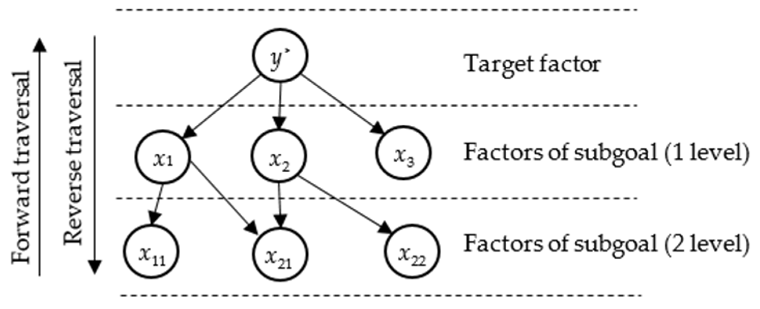
This research is dedicated to solving hierarchical inverse problems of factor formation, i.e., to define the changes in factors of the first and subsequent levels taking into account the input constraints and the selected solution approach in such a way that the target indicator takes a set value. Thus, the initial values for factors of the subgoal of the first (x1, x2, x3) and second (x11, x21, x22) levels were set for the problem as shown in Figure 1, where it was required to determine their changes (Δx1, Δx2, Δx3, Δx11, Δx21, Δx22) in such a way that the target factor was equal to y*.
A separate subproblem indicates the solution of the inverse problem when defining the values of characteristics which form the factor of the higher level. Thus, in Figure 1, the solution of the general problem includes subproblems such as the determination of values Δx1, Δx2, and Δx3 for the development of y*, the calculation of Δx11 and Δx21 for the formation of x1 + Δx1, and the calculation of Δx21 and Δx22 for the formation of x2 + Δx2.
The object-oriented approach is suitable for modeling structures such as graphs and trees [40,41], and its implementation enables the development and flexible modification of readymade software, as well as a reduction in expenses for the realization of new subject-oriented systems owing to the usage of ready-to-use templates.
Testing of the developed algorithm was performed using the example of solving the task of profit generation, which is the most important indicator of enterprise activity.
2.1. Development of Algorithms for Solution of Subproblems
Let us consider the algorithms for solving the subproblems using the example of forming the value of target factor y* (Figure 1), which is calculated on the basis of values of x: y = f (x). The below methods of solving subproblems can be considered.
- Minimizing the sum of squares of argument changes:
- Minimizing the sum of absolute values of arguments:
- Using the coefficients of relative importance and directions of argument changes.
- Involving the coefficients of relative importance for cases with the smallest changes in factors.
To solve the given problems, the usage of iterative algorithms was reviewed; their essence involves executing multiple iterations, where the arguments are changed to some small extent until the solution with preset accuracy is found, and the difference between the current value of the function and the target one increases.
Problems which involve minimizing the sum of squares of changes and the sum of absolute values of changes of the arguments are referred to as optimization problems. Since such problems have a symmetric objective function ) and one constraint, methods that are easier to implement than traditional ones (penalties, Lagrange multipliers, etc.) have been developed. The symmetry of the objective function provides an equal impact on the change in the objective function of each argument, where the problem solves the equation using the direction of the gradient vector.
In order to solve the problem of minimizing the sum of squares of argument changes, we consider the usage of the Landweber algorithm [34], according to which the change in factor i is fulfilled through the following formula:
where α is a small number, defining the step of changing x, and y is the initial value of the resulting indicator.
In the case of minimizing the sum of absolute values at each iteration, the selection of the argument for change (index k) [42] takes place, after which the value of that argument changes according to
The argument for change is chosen on the basis of the value of the partial derivative, i.e., the argument for which the absolute value of the partial derivative is maximum () is defined.
The authors of ref. [42] investigated the one-sweep method, where the solution of the equation with respect to the argument for which the value of the partial derivative is maximum was mentioned. However, testing on a set of models showed that, with nonlinear functions, there was a change in the correlation of values of private derivatives with a change in the arguments to achieve the target value of resultant factors. Thus, iterative change makes it possible to take into account such behavior and obtain a more precise result.
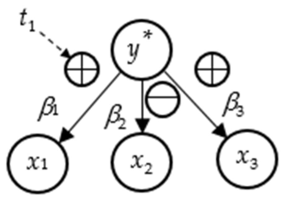
Figure 2 represent the factor tree in the event of using the coefficients of relative importance, which are compliant to proportions of the change in arguments and their directions reflecting the increase or decrease in the argument [43].
The iterative change in arguments, in this case, is expressed as
where t is the direction factor (when t = 1, it is necessary to increase the argument; when t = –1, it is required to decrease the argument), and β is the coefficient of relative importance established by the expert.
This approach to solving problems can lead to situations where the solution cannot be found, thus necessitating an expert to correct the initial data, which is a time-consuming task when the number of arguments is high. A special situation using such an approach with a lesser amount of expert information involves the use of coefficients of relative importance when the change level of factors is low. For instance, in the case of an additive model with an increase in the factor, the solution, in the event of the least adjustment of arguments, will correspond to a positive change of characteristics. To implement this solution, the influence of the argument on a change in the target factor can be analyzed pursuant to the received direction of variable t (see Equation (5)). Another approach is the use of the stochastic algorithm presented in ref. [44]. Within this algorithm, at each iteration, argument x is selected to change by modeling the full group of incompatible events while considering the coefficients of importance as a probability. However, the given algorithm allows determining the solution only in the case of an additive model where the modification was fulfilled.
The inverse problem of defining the value of argument k on iteration i is solved as follows:
Accordingly, unlike the previous algorithm, where the new value is defined by solving the equation with respect to the selected argument, in the presented formula, the step of change is calculated on the basis of a partial derivative through the modifiable variable. Value is defined as the difference between the argument value, calculated by means of solving the equation with respect to it, and the previous argument value . The use of the derivative enabled the ability to exclude the influence of functional dependency.
2.2. Development of Algorithm for Generation of the Resultant Factor of Goal Tree
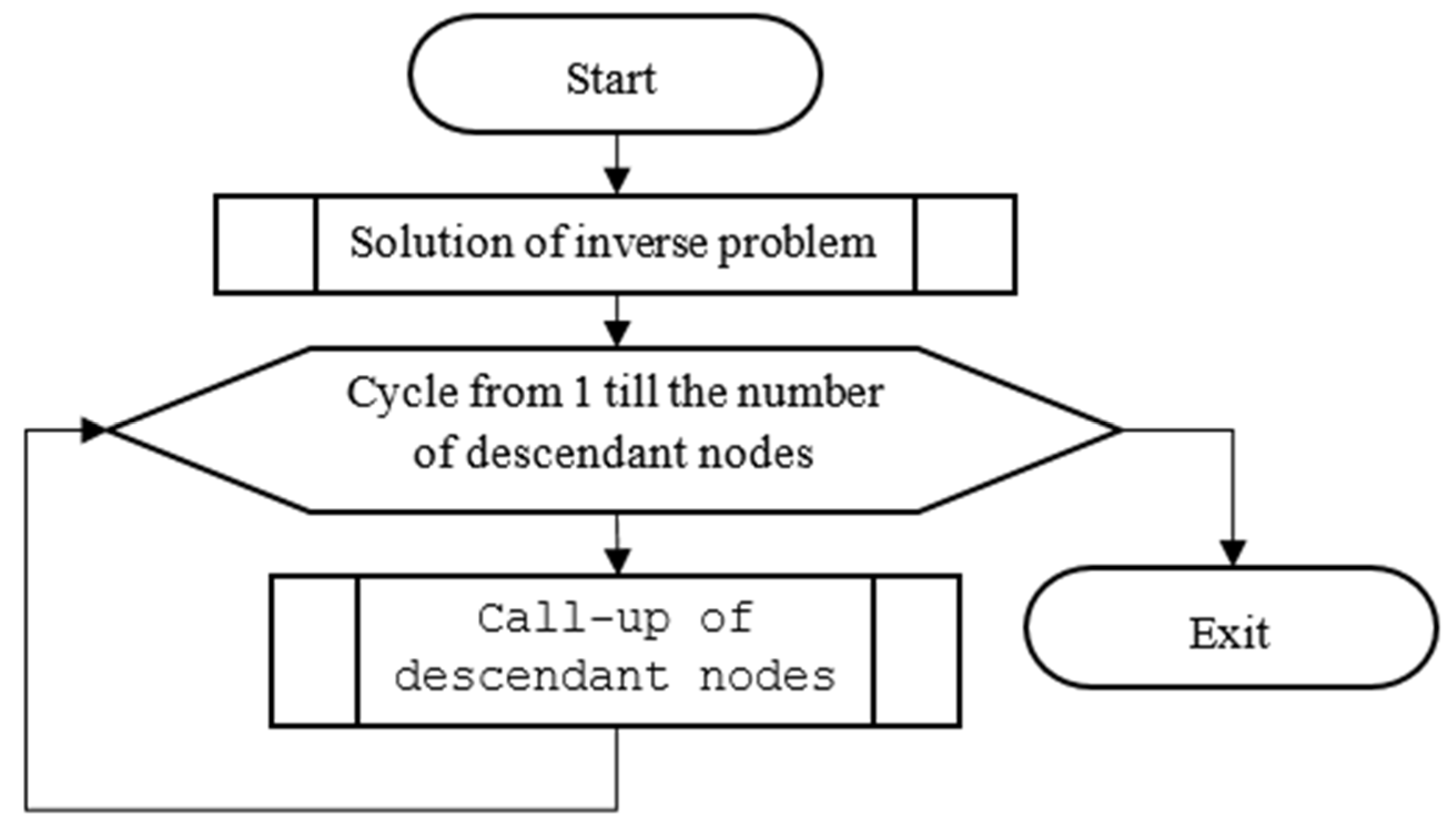
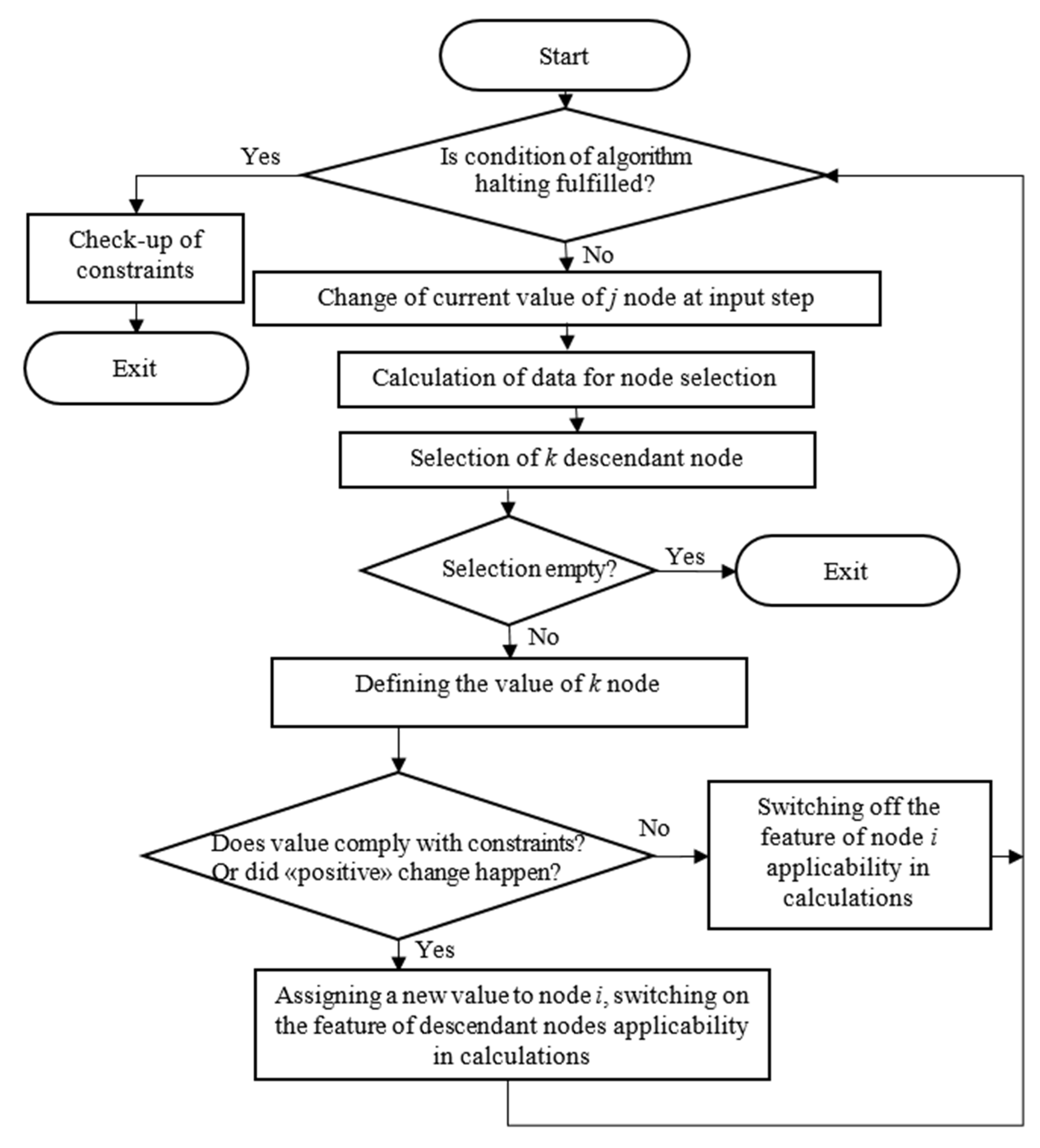
Let us consider the solution to the general problem of defining the resultant factor while taking into account the constraints. In this case, it is required to define the additional characteristics for each factor, i.e., the minimum l and maximum m value, allowing the use of fc in calculations. To traverse the goal tree, the recursive procedure is used (Figure 3), within which the factors are presented in the form of nodes (descendant nodes are characteristics which form the factor of a higher level). The new values of the descendant nodes, calculated using the procedure of solving the inverse problem, become target values for defining the descendant nodes of the subsequent level.
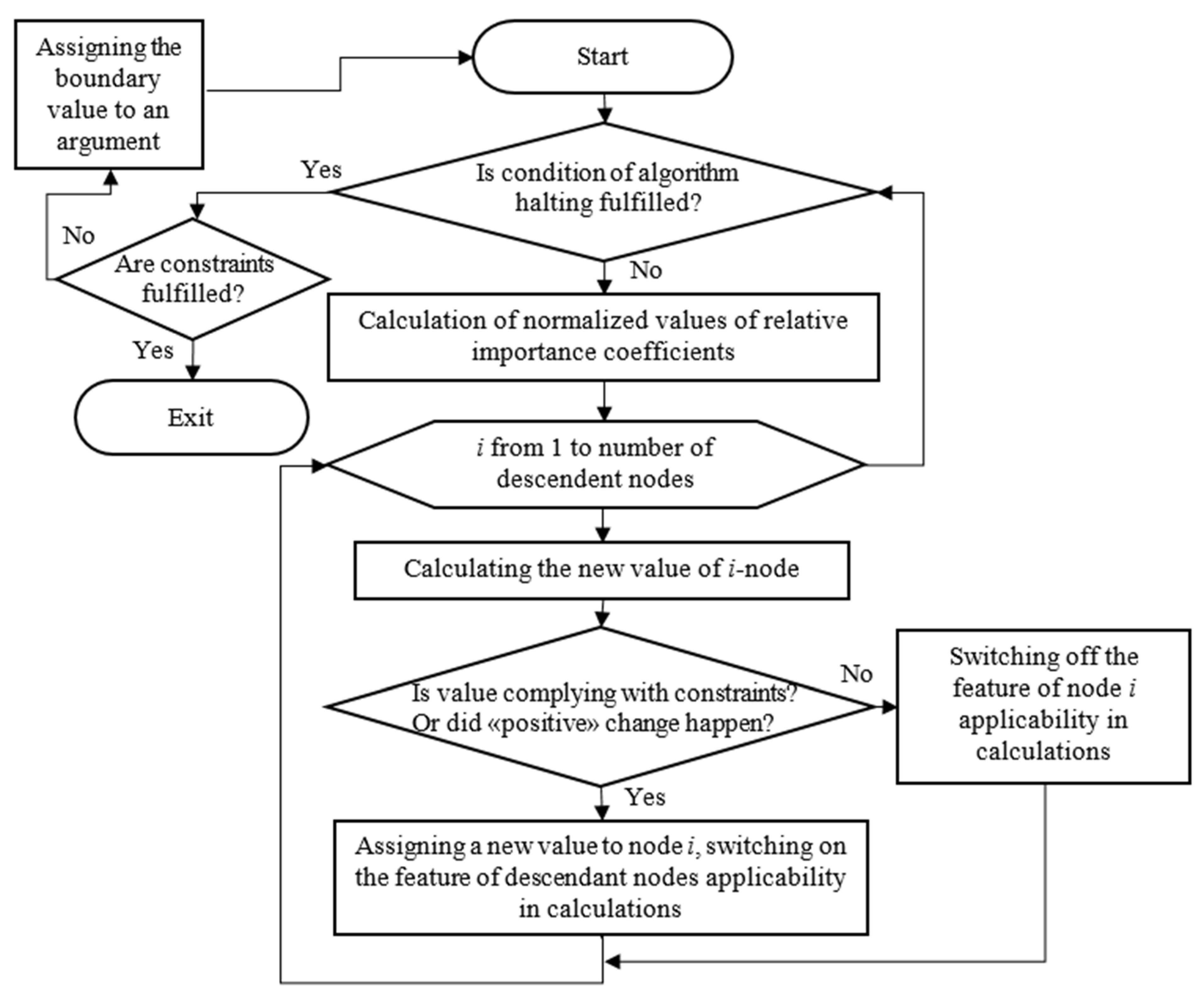
Figure 4 present the general algorithm for solving the inverse problem. The condition for the algorithm halting is the increase in the difference between the target value of the resultant factor and its current value. Calculating the normalized values of importance coefficients is performed by excluding from calculations those nodes for which the values reach the boundary levels. The new value of the node is calculated using Equations (3) and (5), where a “positive” change is understood to be a situation where the value in the current iteration becomes closer to the permissible region in comparison to the previous iteration (the initial value did not satisfy input constraints). For applicability in calculations, this value is set to 1 if a further change in this factor is possible or 0 if this factor cannot be changed. After completion of the algorithm, it is checked for compliance with the constraints. If the value does not comply with the constraints, the closest boundary value is assigned, and the algorithm starts afresh, while a change in this argument does not happen over the course of algorithm execution. Furthermore, checking for the lack of a solution is performed using relative importance coefficients when the input interrelations and directions of change do not allow us to reach the goal.
An algorithm for solving the problem based on the selection of arguments for change is presented in Figure 5. Node j is the top of the tree that represents the factor under formation in the current subproblem. In the stochastic algorithm, the calculation of data for node selection includes normalizing the importance coefficients, which act as probabilities, and the selection of the k node is accomplished by modeling the full group of incompatible events. When minimizing the sum of arguments’ absolute values, the calculation of data includes the calculation of partial derivatives, and the selection of the k node is performed by defining the maximum value of the partial derivative. The value of the k node is determined using Equations (4) and (6).
The novelty of the proposed algorithms (Figure 4 and Figure 5) is in the ability to traverse the factor tree with changes to the indicators and check for constraints. In contrast to existing procedures for solving one-level inverse problems [39], the proposed algorithm makes it possible to find a solution in the case of a large number of arguments and if the initial conditions do not satisfy the constraints.
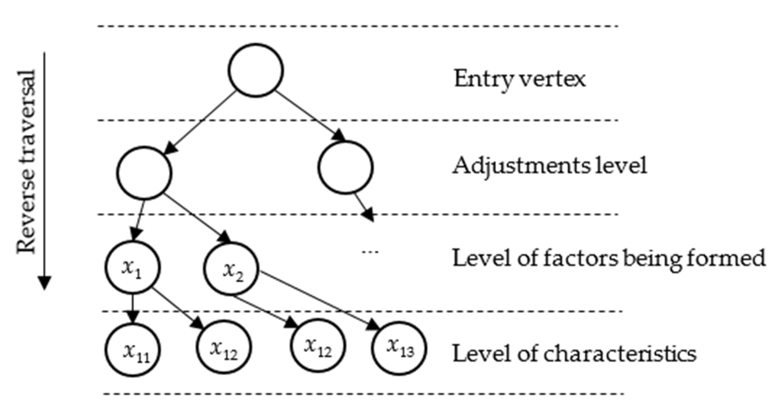
If the same characteristic is used in the calculation of various factors (for example, in Figure 1, the value x21 is used when calculating x1 and x2), an adjustment is made after finding the solution [45,46,47]. For instance, such a situation occurs when the parallel formation of the cost price of different manufacturers takes place, and this cost price, in turn, is defined by the price of the same product. In this case, an adjustment tree is developed, which includes the factors of the goal tree, and the problem is solved while minimizing the sum of squares of argument changes. The adjustment tree is created in the following way (Figure 6):
- On a zero level, there is an entry vertex for the startup position of the tree traversal procedure;
- There are adjustments on a first level, with the number of nodes on this level corresponding to the necessary quantity of adjustments;
- Factors and their characteristics are on the second and third levels.
The problem is solved iteratively; the changes in characteristics are defined in such a way that the sum of squares of changes is minimal, while the values of the factors being formed are equal to those defined using the goal tree.
where n is the number of characteristics referring to the first adjustment, the values of which are subject to the change, m is the number of factors under formation, and is the target value of xi, defined in the process of solving the inverse problem with usage of the goal tree.
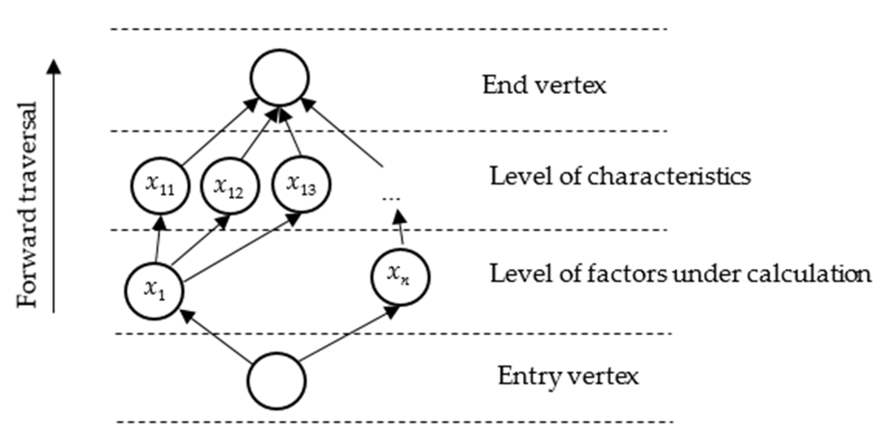
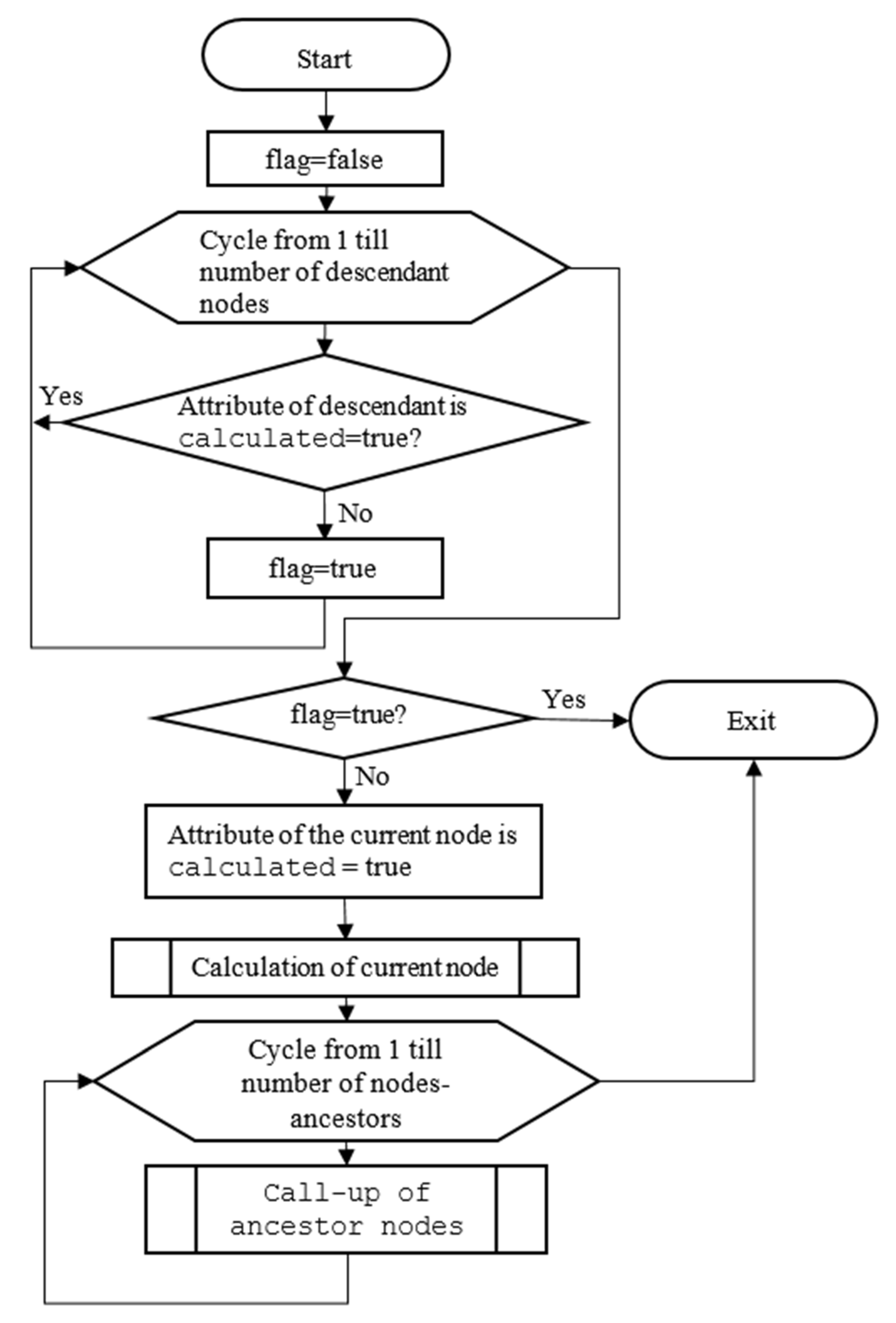
After solving the primary problem and adjustments, the task of results processing may arise, involving the calculation of new values based on existing ones, e.g., defining the total volume of raw materials on the basis of the cost price of different types of products. For this, a graph of results processing is created from the respective nodes (Figure 7). As this problem is direct, the graph is traversed from bottom to top. In this case, the nodes are calculated successively; the end node is fictitious and designed for the startup of the recursive procedure of graph traversal, which implies the calculation of the current vertex only when all its descendants are calculated. For the realization of the traversal procedure, each node has a calculated attribute. At the initial stage, the value “false” is assigned to this attribute. In the course of recursive graph traversal, a change in the attribute value to “true” takes place. An algorithm for calling up the fictitious end node is presented in Figure 8. In this algorithm, the variable “flag” is used, which adopts the value “false” if all descendant nodes of the current node are calculated (the calculation of the current node is only initiated in this case).
Forward traversal can also be used for the traversal of the factor tree when, for example, the solution of an inverse problem is determined on the basis of a direct problem solution.
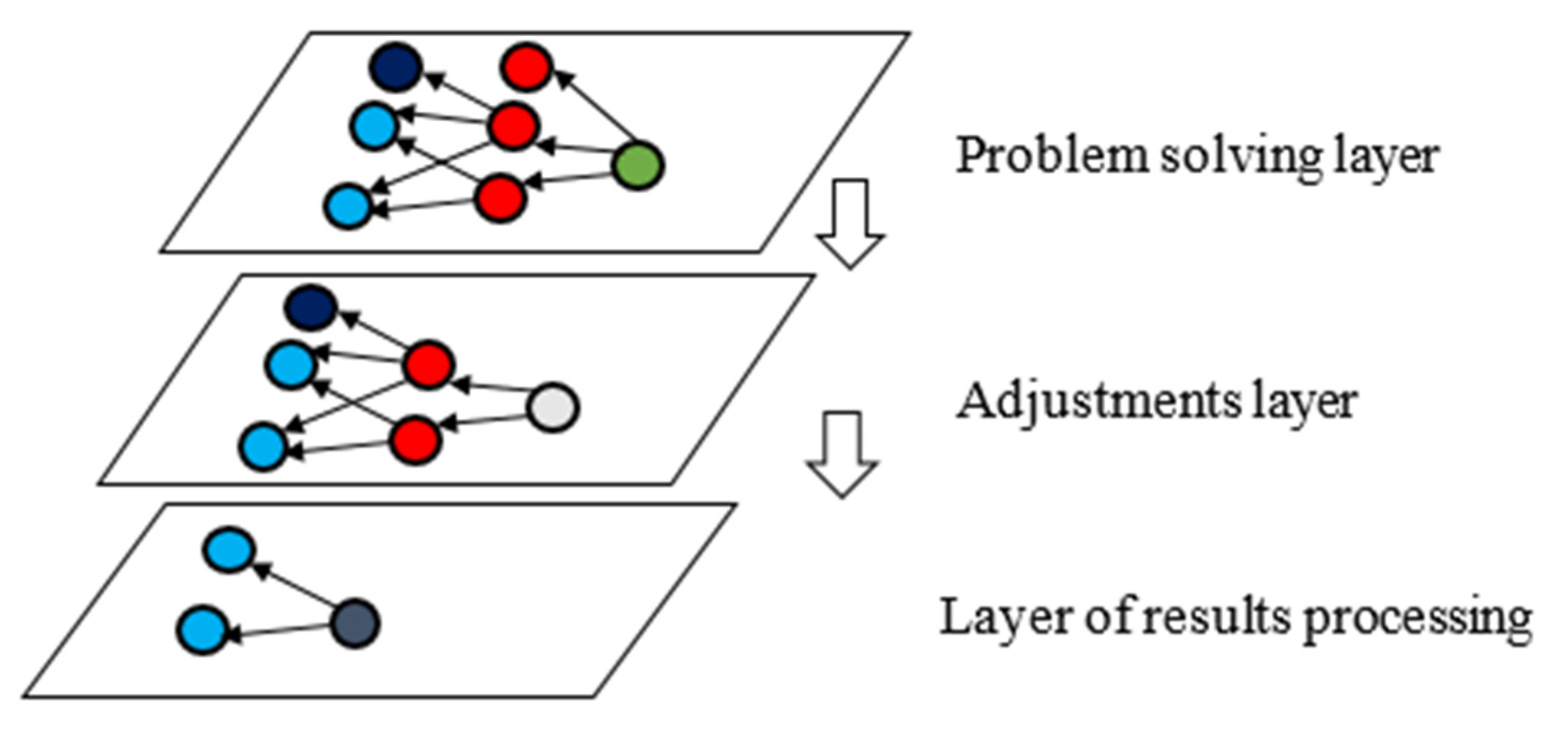
Thus, the solution to the inverse problem includes the traversal of three layers, for which a tree/graph is formed in each case (Figure 9).
2.3. Object-Oriented Architecture
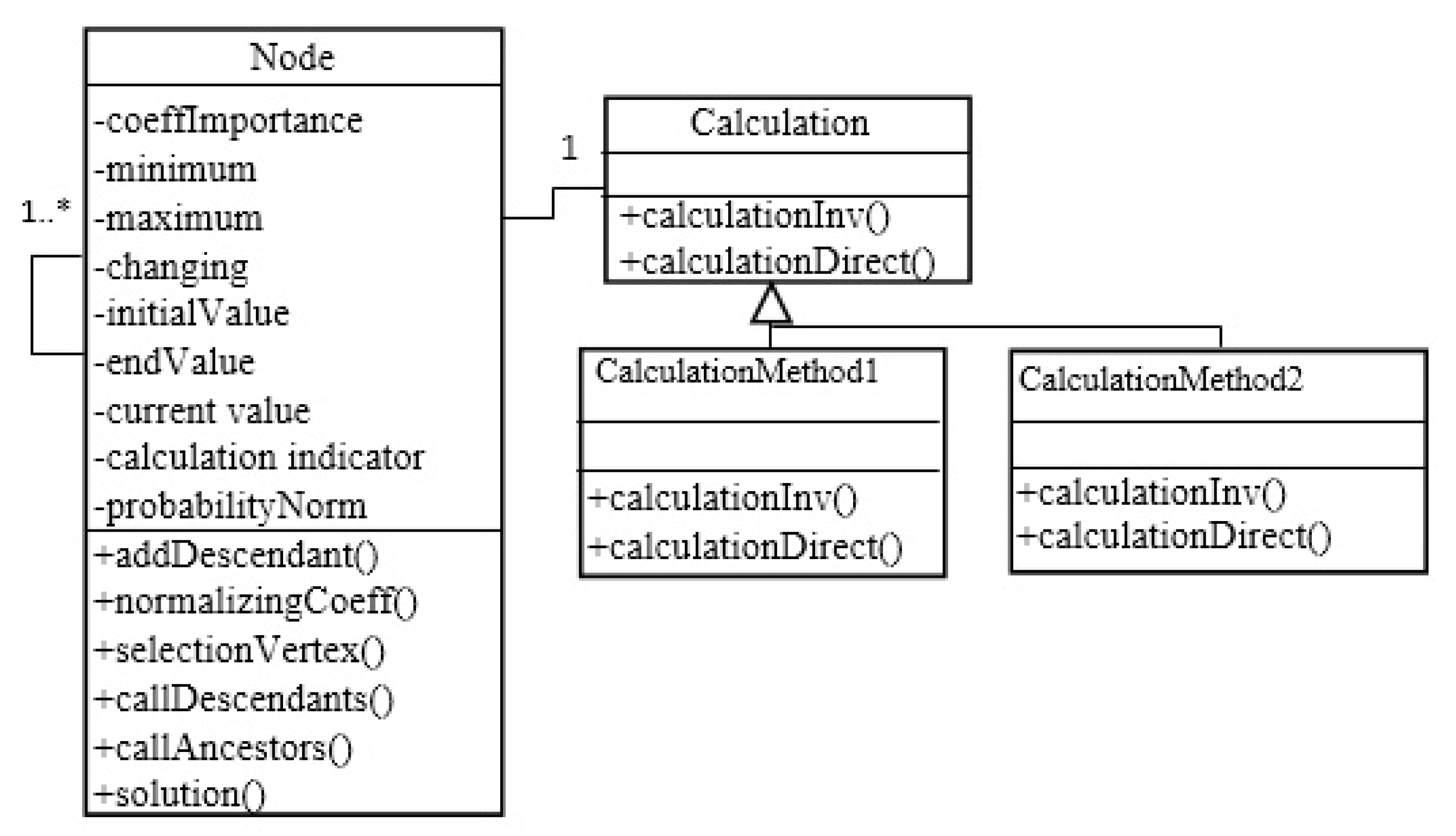
For software implementation of the graph/tree, representation in the form of a multilinked list is used. Each element of this list is an object of the node class, which is capable of referring to any quantity of ancestor nodes and descendant nodes (Figure 10). The class node for solving the problem contains a reference to the abstract class calculation. The realization of algorithms for solving the inverse and direct problems is fulfilled in inheritor class calculation. Each object of the node class contains the link to the inheritor object of the calculation class, whereby the solution path for direct and inverse problems is set as a vertex. For instance, in the method “calculationInv”, Equations (1)–(5) are iteratively realized. The methods «callofDescendants» and «call ofAncestors» are implemented for the recursive traversal of the graph/tree. The algorithm for solving the inverse problem, taking into account the constraints (Figure 4 and Figure 5), is realized in the method “solution”, which is called up during recursive traversal. Figure 10 display the basic attributes of the “node” class (“1..*” means that an object of the node class connects with at least one another object). The object-oriented architecture provides the possibility of flexible modification and expansion of the system, i.e., the addition of new factors, methods for solving inverse problems, etc.
3. Results
3.1. Testing of Iterative Algorithms of Solving the Inverse Tasks
Testing of the developed algorithm was carried out for solving subproblems using the following models most often applied in economic analysis:
- Additive model: y = x1 + x2 + x3 + x4 + x5;
- Multiplicative model (model of product manufacture): y = x1 x2 x3 x4;
- Nonlinear additive model (cost model in inventory management system): y = a1/x1 + b1 x1 + a2/x2 + b2 x2 + a3/x3 + b3 x3;
- Nonlinear multiplicative model (Cobb–Douglas model): y = x1a x2b;
- Multiplicatively additive model (profit model): y = x1−x2−x3−x4.
As an example, the results of solving the problem using the multiplicative model are presented in Table 1 (initial data: x1 = 10, x2 = 26, x3 = 10, x4 = 8; input value of resultant factor = 25,000; positive direction of change for the first, third, and fourth arguments; negative direction of change for the second argument). The value of the Euclidean metric e(x) was calculated to check for compliance of the received solution with the coefficients of relative importance:
where n is the number of arguments.
To solve the problem by minimizing the sum of squares of argument changes and the sum of modules of argument changes, the values of target function g(x) in Equations (1) and (2) were calculated.
The evaluation of compliance with the constraints is defined as the absolute difference between the value of constraint function f(x) and set value y*.
d = |f(x) − y*|.
At the same time, the reduction of step partly contributes to an improvement in the solution by minimizing these characteristics.
While using relative importance coefficients, the application of the stochastic algorithm was considered; Table 1 demonstrate the solution in one iteration. Averaging the solution within a few iterations was also conducive to an increase in accuracy.
For comparison, the factors were also computed using the Excel mathematical package. The received results corroborated the solutions obtained using the mathematical package, optimization models, and classic methods. When using the relative importance coefficients and the directions of argument changes, the values were accurate to the sixth decimal place. When minimizing the sum of squares of argument changes using the iteration algorithm, a smaller deviation from the set value was achieved; when using the function from the mathematical package, a smaller value of the target function was obtained.
The iteration algorithms were also tested with constraints; in particular, an option when the initial values do not comply with the constraints was considered. The received results were compliant with the permissible region.
3.2. Solving the Problem of Profit Generation in a Fast-Food Restaurant
Premised on the developed algorithm, the problem of profit generation was developed in C# language using the Visual Studio environment.
The program’s input data were as follows:
- The initial values of price, cost price, and sales volume for each type of product;
- The importance coefficients, directions of change, minimum and maximum values of profit from sales of products i, price, cost price, and sales volume;
- The target value of total profit;
- The methods of solving the problem included the use of relative importance coefficients and directions of change or the use of relative importance coefficients for values with the smallest change of values, with minimization of the deviation from the initial values;
Two-level and three-level problems were considered. In the case of a two-level problem, the price, cost price, and sales volume for each product were defined to determine the input value of the total profit. When solving the three-level problem, the profit by product name was determined to reach the established consolidated profit before calculating the cost price, sales volume, and price for profit generation.
The program output data were the values of price, cost price, sales volume, and profit by product name according to the input value of the target profit.
The program was tested by calculating the Euclidean distance from set values, solving separate subproblems using the Excel mathematical package, and comparing the values with defined boundaries. For the computational experiments, the real data of a fast-food restaurant (LLC WokiFoodTomsk) were used. Eight popular menu items were selected (Table 2). The information received from the organization included the selling price, cost price, and sales volume.
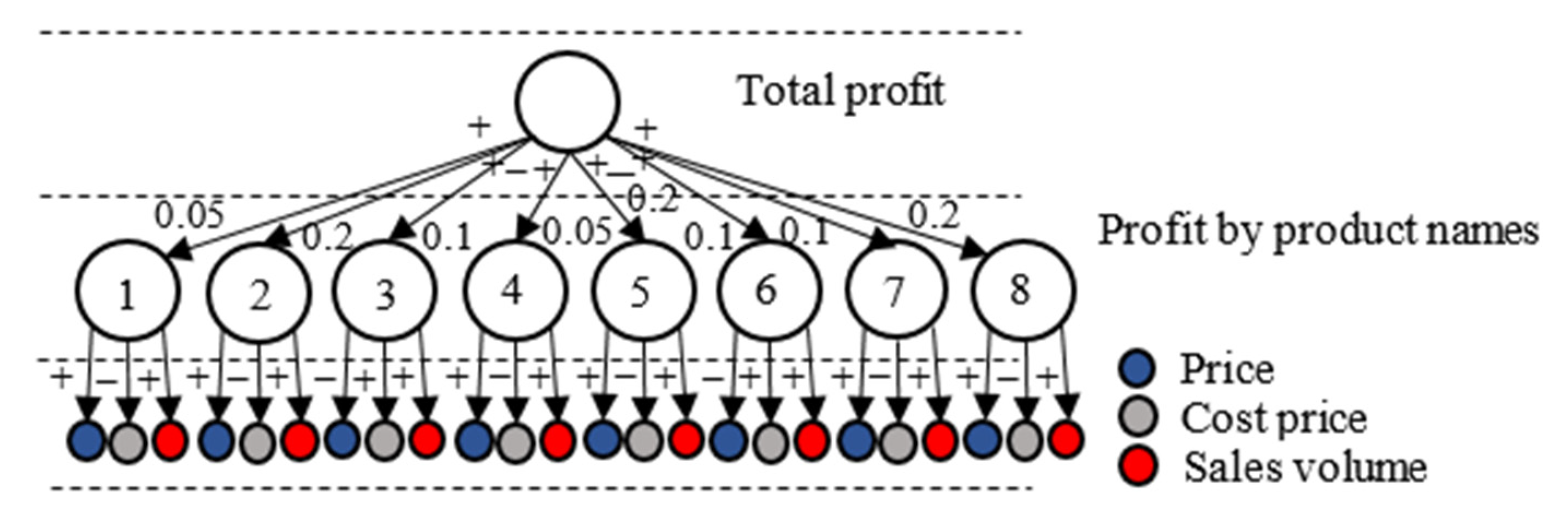
The factor tree, in the case of a three-level model, is presented in Figure 11. This figure demonstrates the use of initial expert information (importance coefficients of profit according to the product name and directions of change); the importance coefficients of price, cost price, and sales volume for all products were equal to 0.5, 0.2, and 0.3, respectively.
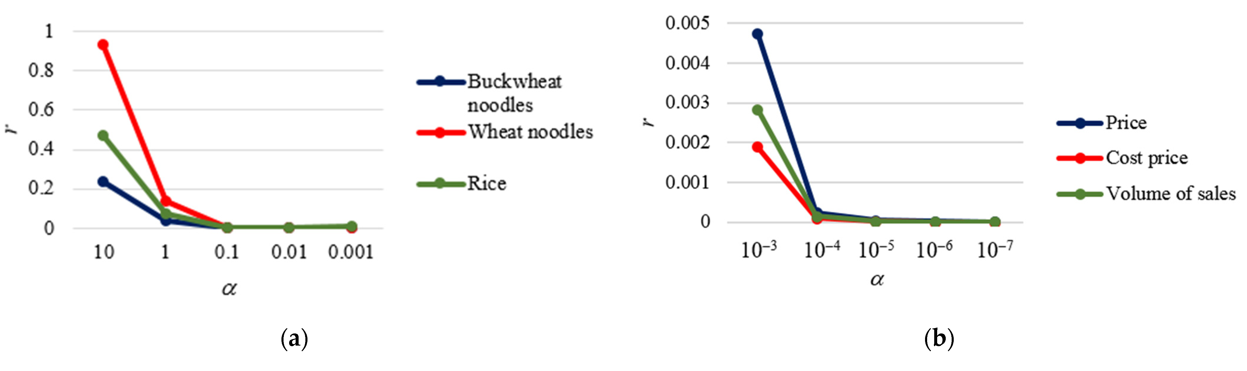
Table 3 present the results of solving the problem of profit generation, equal to RUB 160,000 (the initial value of total profit was RUB 128,718.82). The values of Euclidean distance from set values represent the values close to zero. For comparison purposes, the problem was also solved using a mathematical package. Figure 12a display the value r (depending on the parameter step α), which represents the absolute difference between the value of profit by product name calculated with the help of the algorithm and that defined using the Excel mathematical package. Figure 12b show the dependence of the difference value r on parameter α for the price, cost price, and sales volume of the first item.
Let us also consider the solution to this problem while taking the constraints into account. For the first four items, the lower boundary of cost price was equal to 10, while the upper boundary of price was equal to 115; for the last four products, the upper boundary of price was equal to 120, while the lower boundary of cost price was equal to 15. The results of the solution are presented in Table 4. In this situation, the prices for items 2, 5, and 8 and cost prices for items 2, 5, 7, and 8 (see Table 2 for numbering) were adjusted to the boundary value. Thus, the coefficients of relative importance were corrected, and the received values of change correlation are presented in Figure 13.
When minimizing the sum of squares of factor changes, two characteristics were defined: g(x), the sum of squares of factor changes; d, the absolute difference between the received value of constraint function f (x) and set value y*.
Table 5 present the results of solving the task of generation of total profit, as well as profit by product names, using the proposed algorithm and tools of the mathematical package. By considering a multi-objective problem for the minimization of two parameters, it is possible to conclude that, for the subproblem of the first level, the values of the two factors were smaller than the solution received using the developed algorithm. For the subproblem of the second level, the algorithm enabled a smaller value of the compliance indicator with the set constraints, while the mathematical package provided function g(x).
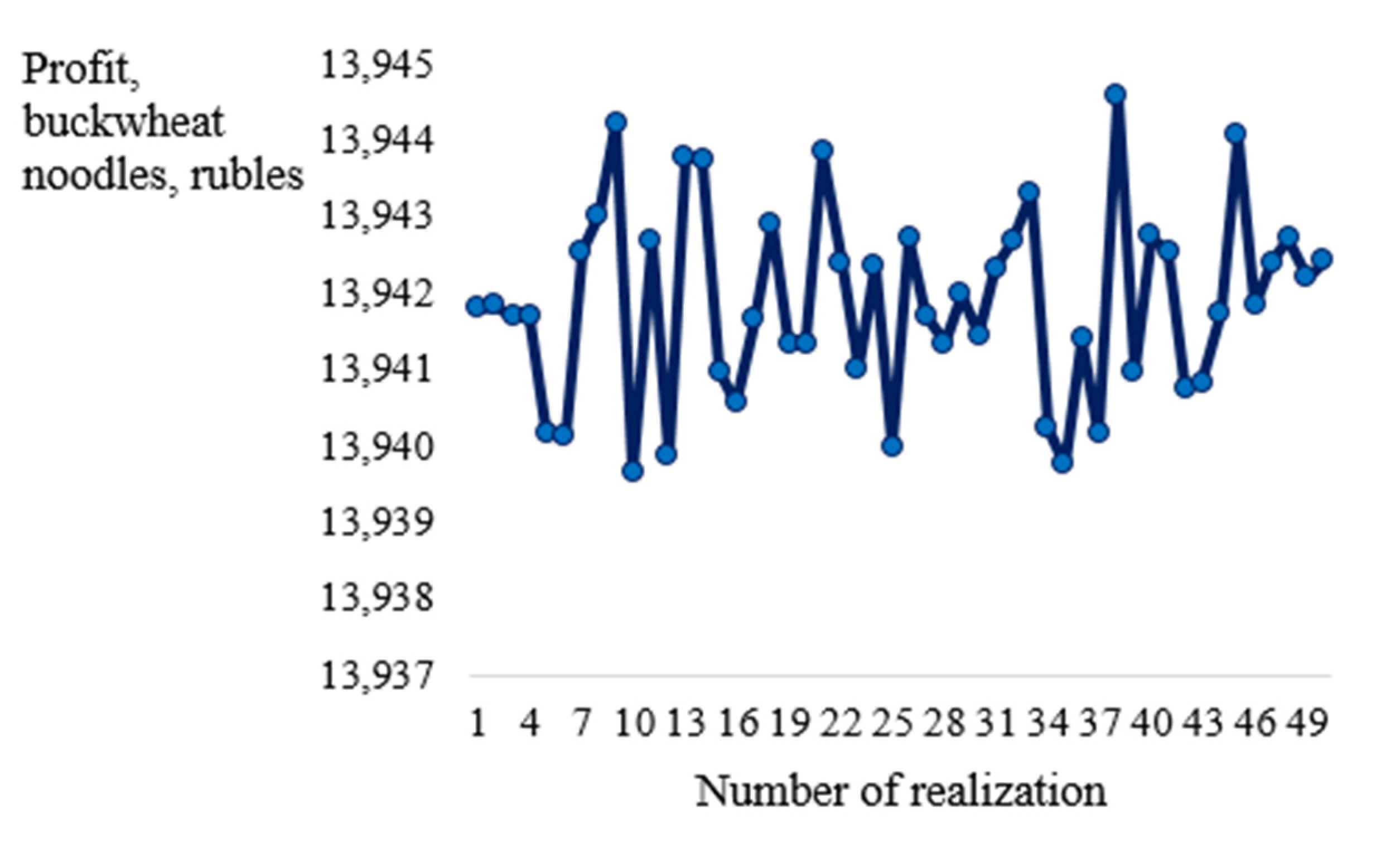
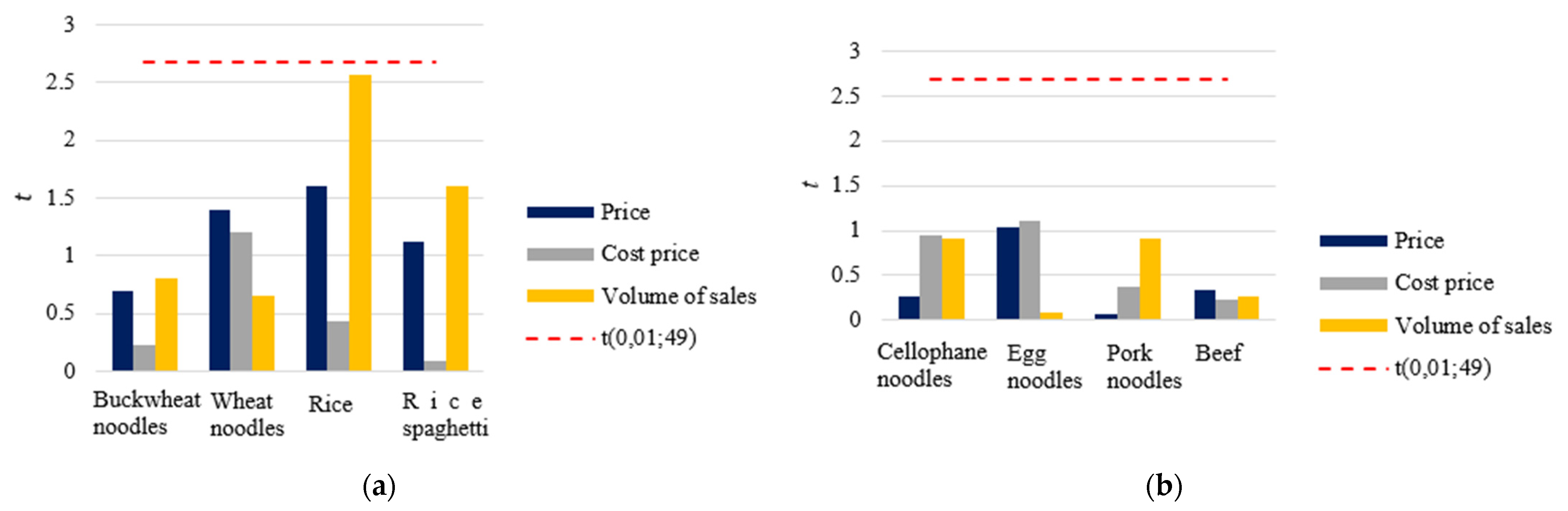
The problem of profit generation was also solved using relative importance coefficients with the help of a stochastic algorithm. The Student’s t-test was used to compare the average sample value with the set value. A total of 50 experiments were conducted for calculations. Thus, Figure 14 present the values of profit by product name with the step size equal to 10−4 (solving the problem of the first level). The problem solved using inverse calculations was taken as the set value. Accordingly, the directions of change were established (Figure 11), which enabled the increase of the resultant value while minimizing the change in the initial data (for profit by product name, price, and sales volume—positive direction of change; for cost price—negative direction of change). Table 6 present the average values, sample variance, and statistical values when solving the problem of the first level. With 49 degrees of freedom and a level of significance of 0.001, the critical value was equal to 3.5. All the calculated values of statistics were lower than the critical value; consequently, the null hypothesis regarding the equality of the average sample value to the set value was not rejected. A step reduction allowed for improving the convergence and decreasing variance. Thus, when solving the subproblems of the second level, the step size was set to 10−7, yielding a maximum variance of 1.44 × 10⁻⁵. Absolute values of the calculated statistical data are presented in Figure 15. All values were lower than the critical value for a level of significance of 0.1 (equal to 2.68). Hence, the null hypothesis regarding the equality of the average value to the set value was not rejected.
4. Discussion
This article developed an algorithm for solving inverse hierarchical problems with constraints. The algorithm differs from existing ones in its ability to solve hierarchical inverse problems with constraints and the use of arguments in a few subproblems. The algorithm was tested by splitting the problem into subproblems and calculating the metrics of deviation from the set values and target functions while also comparing the received results with the solution of subproblems using a mathematical package. Iterative algorithms were used to solve the subproblems, enabling simpler realization, as well as ensuring the possibility to check constraints at each iteration. Accordingly, the iteration formulas of known algorithms were modified; specifically, the stochastic algorithm and the algorithm of solving the problem by minimizing the sum of absolute values of arguments, and procedures for checking compliance with constraints during and after completion of the algorithm were added.
The accuracy of a solution is defined by the step size of the factor change; thus, the results in Figure 12 testify that higher compliance with the solution using the classic method was achieved using a smaller step size (with a step size equal to 10−7, the solution was precise up to the fifth decimal place). The problem was also solved when considering the constraints (Table 3); the obtained values corresponded to the admissible ones.
In the situation of minimizing the sum of squares of argument changes, the solution was evaluated using two criteria: the value of the target function and compliance of the solution with constraints. The results demonstrated in Table 4 show that the use of the algorithm at the second level enabled higher compliance with the constraints, while the solution using the mathematical package allowed defining the solution with a smaller value of the target function.
The modified stochastic algorithm was used to determine the solution when using the relative importance coefficients. The results displayed in Table 5 and Figure 15 speak to the compliance of the results to the problem solved using the algorithm and inverse calculations with established directions of change.
The novelty of the proposed iterative algorithms lies in the possibility of solving the inverse problem for various types of functions, including nonlinear ones. When minimizing the sum of absolute values of arguments, this was achieved by iteratively choosing the argument to change. In the case of the stochastic algorithm, a correction based on the derivative of the constraint function was used.
For the realization of the algorithm, an object-oriented architecture was developed, which enabled the performance of flexible modification and software development. Furthermore, this architecture ensures the stepwise solution of subproblems; at each stage, the specialist uses the results of solving the previous subproblem to determine the input data for solving the next subproblem. The created algorithm was applied to solving the problem of profit generation to prove its applicability.
5. Conclusions
In this work, an algorithm for solving inverse hierarchical problems with constraints was developed on the basis of the recursive traversal of a factor tree with a stepwise iterative solution to the inverse problem. The problem solution included the passage of three layers, for which a separate tree was initiated.
The results of solving the subproblems using a multiplicative model and a real case of fast-food restaurant profit generation were presented.
The results of this work can be useful for decision-making by economic specialists as well as in the field of software development for informational support during decision-making. The results can also be used in other fields for solving similar inverse and optimization tasks.
Future work will aim at developing iterative algorithms for solving optimization problems such as inverse problems with few constraints and inequalities, for linear programming, and for the creation of table models for informational support during decision making.
Funding
This research received no external funding.
Institutional Review Board Statement
Not applicable.
Informed Consent Statement
Not applicable.
Data Availability Statement
Not applicable.
Conflicts of Interest
The authors declare no conflict of interest.
References
- Ferrario, E.; Zioab, E. Goal Tree Success Tree–Dynamic Master Logic Diagram and Monte Carlo simulation for the safety and resilience assessment of a multistate system of systems. Eng. Struct. 2014, 59, 411–433. [Google Scholar] [CrossRef] [Green Version]
- Kuru, S.; Bek, F. Goal-driven blackboard control architecture based on ex partially complete general trees. Knowl-Based Syst. 1990, 2, 236–241. [Google Scholar] [CrossRef]
- Stashchuk, O.; Vitrenko, A.; Kuzmenko, O.; Koptieva, H.; Tarasova, O.; Dovgan, L. Comprehensive System of Financial and Economic Security of the Enterprise. Int. J. Manag. 2020, 11, 330–340. [Google Scholar] [CrossRef]
- Karpovich, O.G.; Diakonova, O.S.; Pozharskaya, E.L.; Grigorenko, V.V. Digital Growth Points of the Region’s Green Economy in Industry 4.0: Finance and Security Issues. In Industry 4.0; Zavyalova, E.B., Popkova, E.G., Eds.; Palgrave Macmillan: Cham, Switzerland, 2021. [Google Scholar] [CrossRef]
- Bredikhina, N.V. Strategic aspects of the production and economic potential of urban investment and construction sector. J. Appl. Eng. Sci. 2021, 19, 483–487. [Google Scholar] [CrossRef]
- Balan, O.; Moskalyk, H.; Peredalo, K.; Hurman, O.; Samarchenko, I.; Revin, F. Using the Pattern Method for the Comprehensive Organization of Recruitment and Selection of Personnel. Int. J. Adv. Res. Eng. Technol. 2020, 11, 290–300. [Google Scholar]
- Odintsov, B.E. Inverse Computations in Formation of Economical Solutions; Finances and Statistics: Moscow, Russia, 2004; p. 192. [Google Scholar]
- Ghobadi, K.; Lee, T.; Mahmoudzadeh, H.; Terekhov, D. Robust inverse optimization. Oper. Res. Lett. 2018, 46, 339–344. [Google Scholar] [CrossRef] [Green Version]
- Aster, R.C.; Borchers, B.; Thurber, C.H. Parameter Estimation and Inverse Problems; Elsevier: Waltham, MA, USA, 2018; p. 355. [Google Scholar] [CrossRef]
- Al Horani, M.; Fabrizio, M.; Favini, A.; Tanabe, H. Inverse Problems for Degenerate Fractional Integro-Differential Equations. Mathematics 2020, 8, 532. [Google Scholar] [CrossRef] [Green Version]
- Antholzer, S.; Haltmeier, M. Discretization of Learned NETT Regularization for Solving Inverse Problems. J. Imaging 2021, 7, 239. [Google Scholar] [CrossRef]
- Zhenga, G.-H.; Zhang, Q.-G. Solving the backward problem for space-fractional diffusion equation by a fractional Tikhonov regularization method. Math. Comput. Simul. 2018, 148, 37–47. [Google Scholar] [CrossRef]
- Yang, X.-J.; Wang, L. A modified Tikhonov regularization method. J. Comput. Appl. Math. 2015, 288, 180–192. [Google Scholar] [CrossRef]
- Ahuja, R.K.; Orlin, J.B. Inverse Optimization, Part 1: Linear Programming and General Problem; MIT: Cambridge, MA, USA, 1998; p. 35. [Google Scholar]
- Boyd, S.; Vandenberghe, L. Convex Optimization; Cambridge University Press: Cambridge, UK, 2004; p. 730. [Google Scholar]
- Ahuja, R.K.; Orlin, J.B. Inverse optimization. Oper. Res. 2001, 49, 771–783. [Google Scholar] [CrossRef] [Green Version]
- Egri, P.; Kis, T.; Kovác, A.; Váncza, J. An inverse economic lot-sizing approach to eliciting supplier cost parameters. Int. J. Prod. Econ. 2014, 149, 80–88. [Google Scholar] [CrossRef] [Green Version]
- Salman, A.K.; Al-Jilaw, A.S. On the Bridge Between Exterior and Interior Penalty Method. J. Phys. Conf. Ser. 2021, 1818, 012146. [Google Scholar] [CrossRef]
- Dai, Z.; Wen, F. Some improved sparse and stable portfolio optimization problems. Financ. Res. Lett. 2018, 27, 46–52. [Google Scholar] [CrossRef]
- Kalaiarasi, K.; Sumathi, M.; Henrietta, H.M.; Raj, A.S. Determining the Efficiency of Fuzzy Logic EOQ Inventory Model with Varying Demand in Comparison with Lagrangian and Kuhn-Tucker Method Through Sensitivity Analysis. J. Model Based Res. 2020, 1, 1–12. [Google Scholar] [CrossRef]
- Nie, D.; Qu, T.; Liu, Y.; Li, C.; Huang, G.Q. Improved augmented Lagrangian coordination for optimizing supply chain configuration with multiple sharing elements in industrial cluster. Ind. Manag. Data Syst. 2019, 110, 743–773. [Google Scholar] [CrossRef] [Green Version]
- Tsipianitis, A.; Tsompanakis, Y. Improved Cuckoo Search algorithmic variants for constrained nonlinear optimization. Adv. Eng. Softw. 2020, 149, 102865. [Google Scholar] [CrossRef]
- Mohammadi, M.; Musa, S.N.; Bahreininejad, A. Optimization of mixed integer nonlinear economic lot scheduling problem with multiple setups and shelf life using metaheuristic algorithms. Adv. Eng. Softw. 2014, 78, 41–51. [Google Scholar] [CrossRef]
- Solanki, R.; Shah, N.; Shah, J.; Chaudhari, S. Portfolio Management using Beetle Swarm Optimization with Penalty Method. In Proceedings of the 6th International Conference on Inventive Computation Technologies, Coimbatore, India, 20–22 January 2021; pp. 680–685. [Google Scholar] [CrossRef]
- Lee, C.-T.; Chang, J.-Y.J. A Workspace-Analysis-Based Genetic Algorithm for Solving Inverse Kinematics of a Multi-Fingered Anthropomorphic Hand. Appl. Sci. 2021, 11, 2668. [Google Scholar] [CrossRef]
- Darabia, A.; Bagheri, M.; Gharehpetian, G.B. Dual feasible direction-finding nonlinear programming combined with metaheuristic approaches for exact overcurrent relay coordination. Int. J. Electr. Power Energy Syst. 2020, 114, 105420. [Google Scholar] [CrossRef]
- Ye, N.; Roosta-Khorasani, F.; Cui, T. Optimization Methods for Inverse Problems. MATRIX Ann. 2017, 2, 121–140. [Google Scholar] [CrossRef] [Green Version]
- Li, D.-G.; Fu, J.-L.; Yang, F.; Li, X.-X. Landweber Iterative Regularization Method for Identifying the Initial Value Problem of the Rayleigh–Stokes Equation. Fractal Fract. 2021, 5, 193. [Google Scholar] [CrossRef]
- Aspri, A.; Banert, S.; Öktem, O.; Scherzer, O. A Data-Driven Iteratively Regularized Landweber Iteration. Numer. Funct. Anal. Optim. 2020, 41, 1190–1227. [Google Scholar] [CrossRef] [Green Version]
- Yang, F.; Sun, Q.-X.; Li, X.-X. Three Landweber iterative methods for solving the initial value problem of time-fractional diffusion-wave equation on spherically symmetric domain. Inverse Probl. Sci. Eng. 2021, 29, 2306–2356. [Google Scholar] [CrossRef]
- Jose, J.; Rajan, M.P. A Simplified Landweber Iteration for Solving Nonlinear Ill-Posed Problems. Int. J. Appl. Comput. Math. 2017, 3, 1001–1018. [Google Scholar] [CrossRef]
- Qi-Nian, J. On the iteratively regularized gauss-newton method for solving nonlinear Ill-posed problems. Math. Comput. 2000, 69, 1603–1623. [Google Scholar] [CrossRef] [Green Version]
- Riahi, M.K. An Approach to Improve Ill-Conditioned Steepest Descent Methods, Application to a Parabolic Optimal Control Problem via Time Domain Decomposition. 2014. Available online: https://hal.inria.fr/hal-00974285v1/document (accessed on 6 June 2014).
- Gribanova, E.B. Development of iterative algorithms for solving the inverse problem using inverse calculations. E-Eur. J. Enterp. Technol. 2020, 4, 27–34. [Google Scholar] [CrossRef]
- Tsvetkov, M.A. “Reciprocal network” method of improving the structure of credit-deposit base in commercial banks. Econ. Manag. 2007, 1, 139–141. [Google Scholar]
- Vishtak, O.V.; Shtyrova, I.A. Usage of inverse calculations technology in monitoring the quality of supplementary education in higher educational establishment. Vestn. Astrakhan State Tech. Univ. Sci. J. 2014, 2, 67–73. [Google Scholar]
- Barmina, E.A.; Kviatkovskaia, I.I. Monitoring the quality of commercial organization. Structuring of indicators. Implementation of cognitive maps. Vestn. Astrakhan State Tech. Univ. Sci. J. 2010, 2, 15–20. [Google Scholar]
- Blyumin, S.L.; Borovkova, G.S. Practicing the analysis of finite changes and the method of inverse calculations in management systems and systems of decision support. Control. Sci. 2018, 6, 29–34. [Google Scholar] [CrossRef]
- Odintsov, B.E.; Romanov, A.N. Iterative method of optimizing the enterprise management by means of inverse computations. Bull. Financ. Univ. 2014, 2, 60–73. [Google Scholar] [CrossRef]
- Tiacci, L. Object-Oriented Event-Graph modeling formalism to simulate manufacturing systems in the Industry 4.0 era. Simul. Model. Pract. Theory 2019, 99, 102027. [Google Scholar] [CrossRef]
- Chen, G.; Rui, X.; Gu, J.; Zeng, X.; Liu, X. Development of an object-oriented framework for the vibration characteristic computation of multibody systems. Adv. Eng. Softw. 2020, 148, 102874. [Google Scholar] [CrossRef]
- Gribanova, E.B. Algorithm for solving the inverse problems of economic analysis in the presence of limitations. EUREKA Phys. Eng. 2020, 1, 70–78. [Google Scholar] [CrossRef] [Green Version]
- Gribanova, E.B. An Iterative Algorithm for Solving Inverse Problems of Economic Analysis Using Weighting Factors. In Advances in Engineering Research; Nova Publishers: New York, NY, USA, 2021; pp. 49–79. [Google Scholar]
- Gribanova, E.B. Stochastic algorithms of solving the inverse problems of economic analysis with constraints. Proc. TUSUR Univ. Tomsk. State Univ. Control. Syst. Radioelectron. 2016, 4, 112–116. [Google Scholar] [CrossRef]
- Gribanova, E.B. Construction of Algorithms for Solving the Inverse Problem when using Indicators in Several Calculation Functions. E-Eur. J. Enterp. Technol. 2022, 1, 44–50. [Google Scholar] [CrossRef]
- Gribanova, E.B. Algorithms for Solving Inverse Problems of Simulation Modeling. Int. J. Comput. 2021, 3, 433–439. [Google Scholar] [CrossRef]
- Gribanova, E.B.; Savitsky, A.S. Algorithm for Estimating the Time of Posting Messages on Vkontakte Online Social Network. Int. J. Inf. Technol. Secur. 2020, 1, 3–14. [Google Scholar]
Figure 1.
Factor tree.

Figure 2.
The task with coefficients of relative importance and directions of the changes in arguments.
Figure 2.
The task with coefficients of relative importance and directions of the changes in arguments.

Figure 3.
The procedure for traversing the tree: calling up descendant nodes.

Figure 4.
Algorithm for solving the inverse problem.

Figure 5.
Algorithm for solving the inverse problem when selecting the node for change.

Figure 6.
Adjustment tree.

Figure 7.
Graph of results processing.

Figure 8.
Algorithm of forward graph traversal.

Figure 9.
Problem-solving layers.

Figure 10.
Structure of classes.

Figure 11.
Factor tree for the problem of profit generation.

Figure 12.
Dependence of difference d on parameter α: (a) first level; (b) second level.

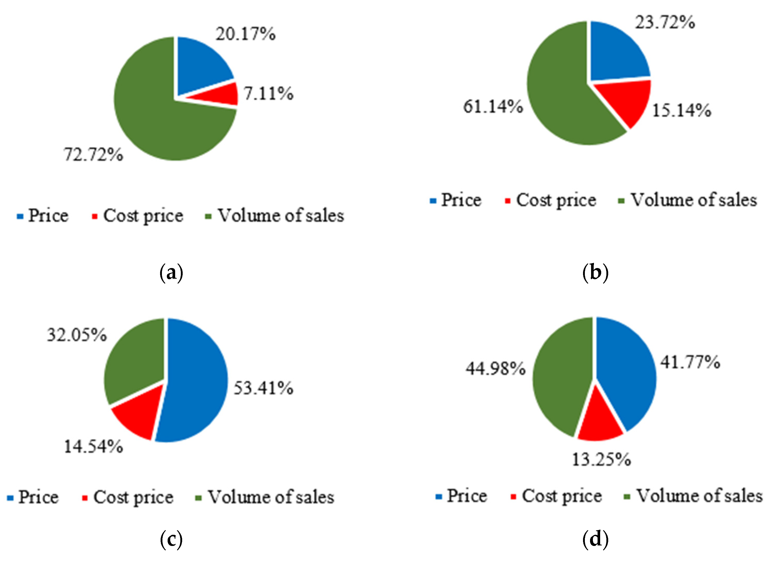
Figure 13.
Correlation of factor changes: (a) wheat noodles; (b) cellophane noodles; (c) pork tenderloin; (d) beef.
Figure 13.
Correlation of factor changes: (a) wheat noodles; (b) cellophane noodles; (c) pork tenderloin; (d) beef.

Figure 14.
Change in product profit as a function of the number of realizations.

Figure 15.
Calculated values of statistics: (a) for the first four items; (b) for the last four items.
Figure 15.
Calculated values of statistics: (a) for the first four items; (b) for the last four items.


Table 1.
The results of computational experiments for multiplicative model.
| Method of Solution | Tool | Value of Factor | |||||
|---|---|---|---|---|---|---|---|
| x1 | x2 | x3 | x4 | e(x)/g(x) | d | ||
| Using relative importance coefficients and directions of change | Iteration algorithm, α = 10−6 | 11.278844 | 25.040867 | 10.639422 | 8.319711 | 1.7 × 10⁻⁵ | 0.013 |
| Mathematical package | 11.278843 | 25.040868 | 10.639421 | 8.319711 | 5 × 10⁻⁸ | 0.0081 | |
| Using relative importance coefficients | Iteration algorithm, α = 10−8 | 10.90183 | 26.67648 | 10.45079 | 8.22552 | 1.8 × 10⁻⁴ | 1.6 × 10⁻⁴ |
| Mathematical package | 10.90182 | 26.67637 | 10.45091 | 8.22546 | 2.5 × 10⁻¹¹ | 7 × 10⁻⁴ | |
| Minimizing the sum of squares of argument changes | Iteration algorithm, α = 10−13 | 10.5131 | 26.20162 | 10.5131 | 8.63279 | 0.967594 | 3.5 × 10⁻⁶ |
| Mathematical package | 10.51512 | 26.20672 | 10.51512 | 8.62778 | 0.967533 | 1.2 × 10⁻³ | |
| Minimizing the sum of modules of argument changes | Iteration algorithm, α = 10−12 | 0 | 0 | 0 | 9.61538 | 1.61538 | 3 × 10⁻⁵ |
| Mathematical package | 0 | 0 | 0 | 9.61538 | 1.61538 | 10−9 | |
Table 2.
Input data.
| № | Product | Selling Price | Cost Price | Sales Volume | Profit |
|---|---|---|---|---|---|
| 1 | Buckwheat noodles | 100 | 19.1 | 153 | 12,377.7 |
| 2 | Wheat noodles | 100 | 15.29 | 234 | 19,822.14 |
| 3 | Rice | 100 | 12.025 | 280 | 24633 |
| 4 | Rice spaghetti | 100 | 23.94 | 131 | 9963.86 |
| 5 | Cellophane noodles | 100 | 27.77 | 153 | 11,051.19 |
| 6 | Egg noodles | 100 | 17.25 | 387 | 32,024.25 |
| 7 | Pork tenderloin | 70 | 21.08 | 147 | 7191.24 |
| 8 | Beef | 90 | 24.52 | 178 | 11,655.44 |
Table 3.
The calculated values of factors when using relative importance coefficients and directions of change (for the first level, α = 10−4; for the second level, α = 10−6).
Table 3.
The calculated values of factors when using relative importance coefficients and directions of change (for the first level, α = 10−4; for the second level, α = 10−6).
| Product | Selling Price, Rubles | Cost Price, Rubles | Sales Volume | Profit, Rubles | e(x) | d |
|---|---|---|---|---|---|---|
| Buckwheat noodles | 109.625 | 15.25 | 158.775 | 14,984.465 | 10−8 | 2.8 × 10⁻⁵ |
| Wheat noodles | 126.048 | 4.871 | 249.629 | 30,249.2 | 9.96 × 10⁻⁹ | 10−5 |
| Rice | 85.175 | 17.955 | 288.895 | 19,419.47 | 9.99 × 10⁻⁹ | 1.6 × 10⁻⁴ |
| Rice spaghetti | 110.942 | 19.563 | 137.565 | 12,570.625 | 1.02 × 10⁻⁸ | 9.9 × 10⁻⁵ |
| Cellophane noodles | 136.211 | 13.286 | 174.726 | 21,478.25 | 1.01 × 10⁻⁸ | 1.3 × 10⁻⁵ |
| Egg noodles | 89.592 | 21.413 | 393.245 | 26,810.72 | 1.02 × 10⁻⁸ | 8.4 × 10⁻⁷ |
| Pork tenderloin | 90.648 | 12.821 | 159.389 | 12,404.77 | 10−8 | 6.8 × 10⁻⁵ |
| Beef | 122.978 | 11.329 | 197.786 | 22,082.5 | 1.01 × 10⁻⁸ | 7.5 × 10⁻⁵ |
Table 4.
The calculated value of factors, provided there are constraints.
| Product | Selling Price | Cost Price | Volume of Sales | Profit |
|---|---|---|---|---|
| Buckwheat noodles | 109.625 | 15.250 | 158.775 | 14,984.465 |
| Wheat noodles | 115 | 10 | 288.088 | 30,249.200 |
| Rice | 85.175 | 17.955 | 288.895 | 19,419.470 |
| Rice spaghetti | 110.942 | 19.563 | 137.565 | 12,570.625 |
| Cellophane noodles | 120 | 15 | 204.555 | 21,478.250 |
| Egg noodles | 89.592 | 21.413 | 393.245 | 26,810.720 |
| Pork tenderloin | 92.336 | 15 | 160.401 | 12,404.770 |
| Beef | 120 | 15 | 210.310 | 22,082.500 |
Table 5.
Results of solving the problem when minimizing the sum of squares of argument changes.
| Subproblem | Solution with the Help of Program | Solution with the Help of Excel Package | ||
|---|---|---|---|---|
| g(x) | d | g(x) | d | |
| Generation of total profit | 122,314,059.014985 | 0.003995 | 122,315,034.395265 | 0.128719 |
| Profit generation, buckwheat noodles | 271.05273 | 2.9 × 10⁻⁵ | 270.8571151 | 6 × 10⁻³ |
| Profit generation, wheat noodles | 138.413805 | 4.8 × 10⁻⁵ | 138.3721408 | 3 × 10⁻⁴ |
| Profit generation, rice | 130.395605 | 1.5 × 10⁻⁴ | 130.3673111 | 5 × 10⁻⁴ |
| Profit generation, rice spaghetti | 346.375331 | 1.6 × 10⁻⁵ | 345.9028259 | 4.3 × 10⁻⁴ |
| Profit generation, cellophane noodles | 275.231678 | 8.8 × 10⁻⁵ | 274.8970648 | 2.3 × 10⁻⁴ |
| Profit generation, egg noodles | 63.420252 | 2.8 × 10⁻⁴ | 63.41656061 | 2 × 10⁻² |
| Profit generation, pork tenderloin | 377.790356 | 10−4 | 377.1783217 | 3 × 10⁻⁴ |
| Profit generation, beef | 216.896854 | 1.4 × 10⁻⁴ | 216.7093108 | 4.6 × 10⁻⁴ |
Table 6.
Statistical values of Student′s t-test.
| Factor | Profit by Name | |||||||
|---|---|---|---|---|---|---|---|---|
| Buckwheat Noodles | Wheat Noodles | Rice | Rice Spaghetti | Cellophane Noodles | Egg Noodles | Pork Tenderloin | Beef | |
| Average value | 13,941.89 | 26,078.17 | 27,760.93 | 11,527.87 | 173,07.59 | 35,151.90 | 10,319.21 | 17,912.45 |
| Sample variance | 1.54 | 4.44 | 3.21 | 1.56 | 3.10 | 2.91 | 3.34 | 2.58 |
| Values received from inverse calculations | 13,941.76 | 26,078.38 | 27,761.12 | 11,527.92 | 17,307.43 | 35,152.37 | 10,319.36 | 17,911.68 |
| Value of test statistics | 0.745774 | −0.70121 | −0.74422 | −0.29017 | 0.641834 | −1.92211 | −0.56969 | 3.387541 |
Publisher’s Note: MDPI stays neutral with regard to jurisdictional claims in published maps and institutional affiliations. |
© 2022 by the author. Licensee MDPI, Basel, Switzerland. This article is an open access article distributed under the terms and conditions of the Creative Commons Attribution (CC BY) license (https://creativecommons.org/licenses/by/4.0/).
Share and Cite
MDPI and ACS Style
Gribanova, E. Elaboration of an Algorithm for Solving Hierarchical Inverse Problems in Applied Economics. Mathematics 2022, 10, 2779. https://doi.org/10.3390/math10152779
AMA Style
Gribanova E. Elaboration of an Algorithm for Solving Hierarchical Inverse Problems in Applied Economics. Mathematics. 2022; 10(15):2779. https://doi.org/10.3390/math10152779
Chicago/Turabian StyleGribanova, Ekaterina. 2022. "Elaboration of an Algorithm for Solving Hierarchical Inverse Problems in Applied Economics" Mathematics 10, no. 15: 2779. https://doi.org/10.3390/math10152779
Note that from the first issue of 2016, this journal uses article numbers instead of page numbers. See further details here.