
Application of Monte Carlo Simulation to Study the Probability of Confidence Level under the PFMEA’s Action Priority


Abstract
:1. Introduction
2. Literature Review
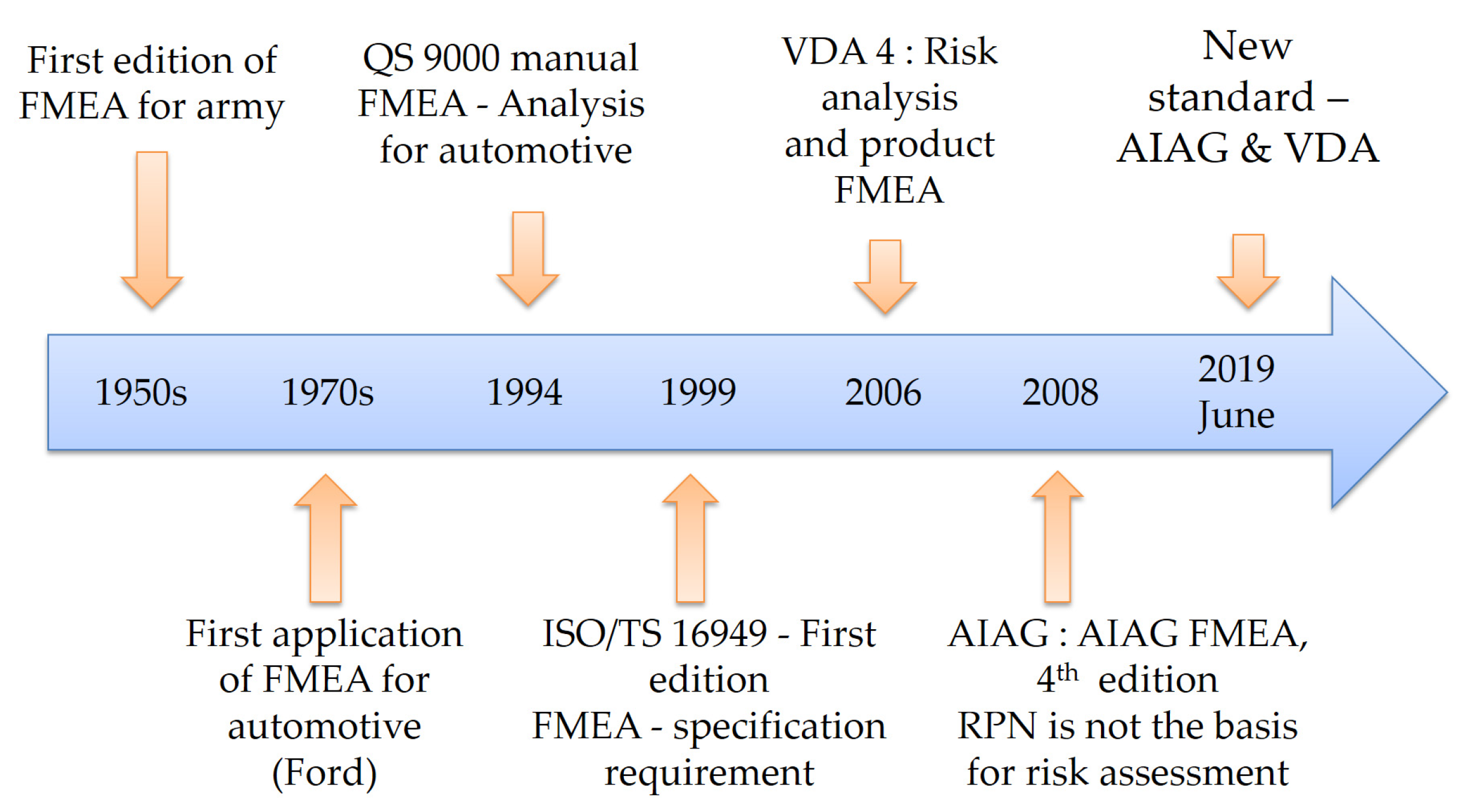
2.1. Failure Mode and Effects Analysis (FMEA)
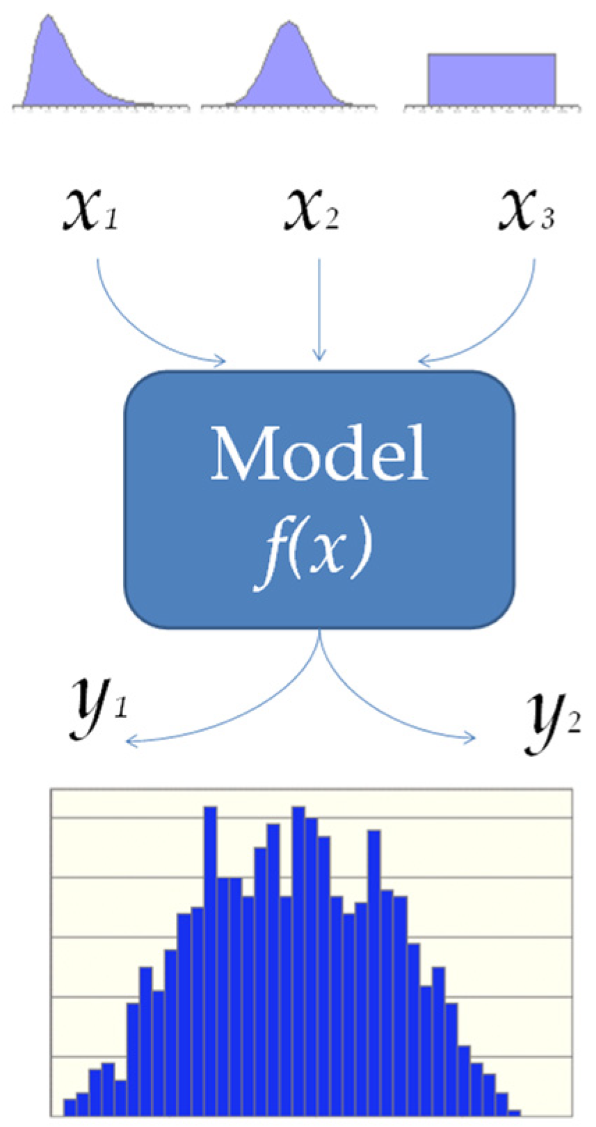
2.2. Monte Carlo Simulation
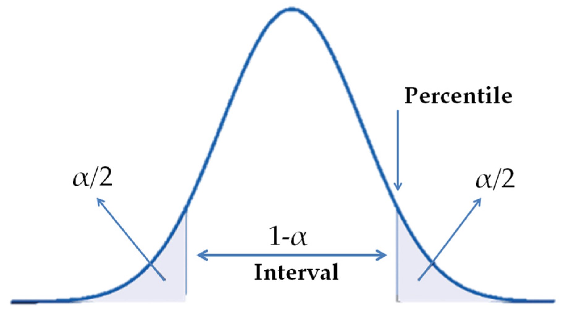
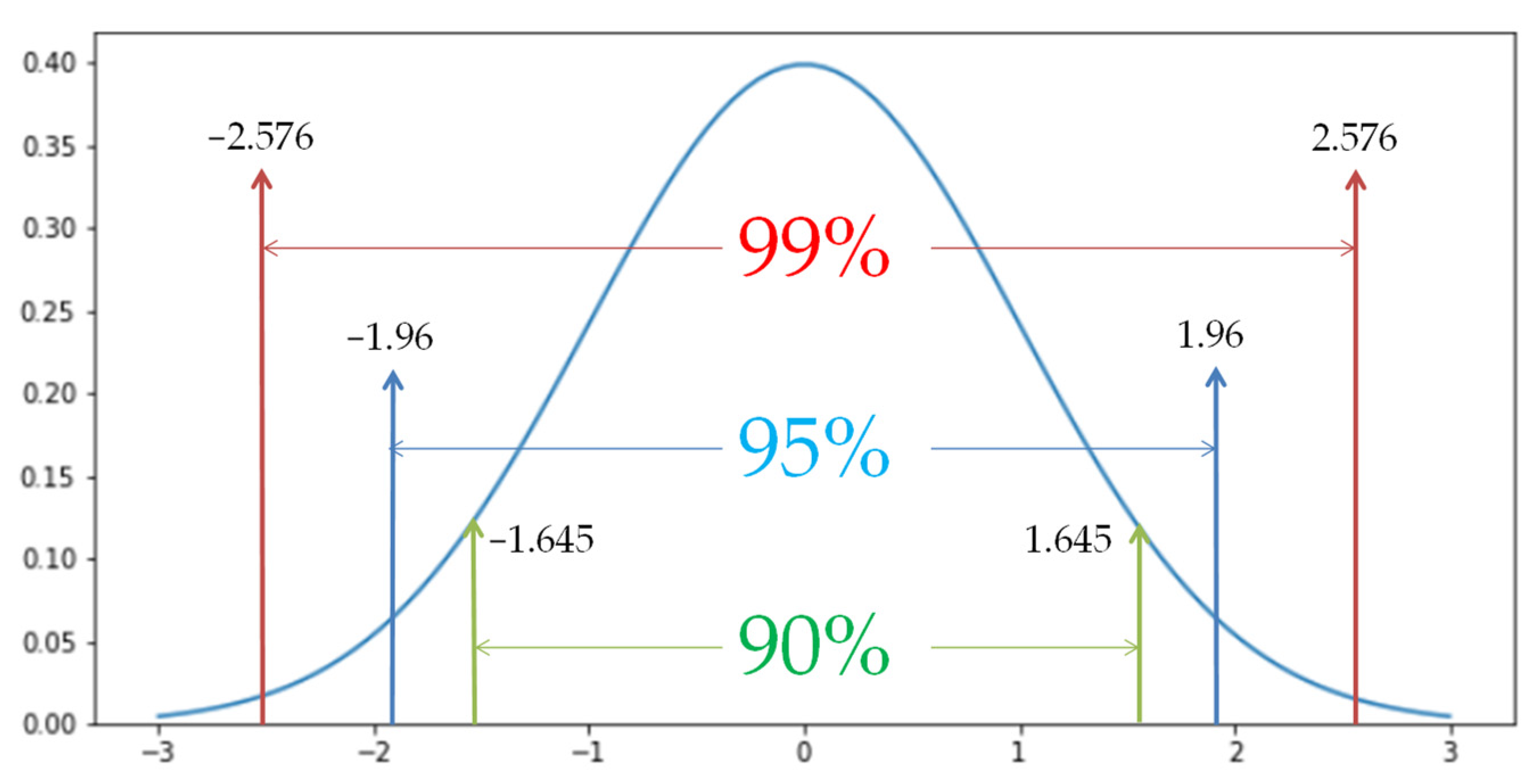
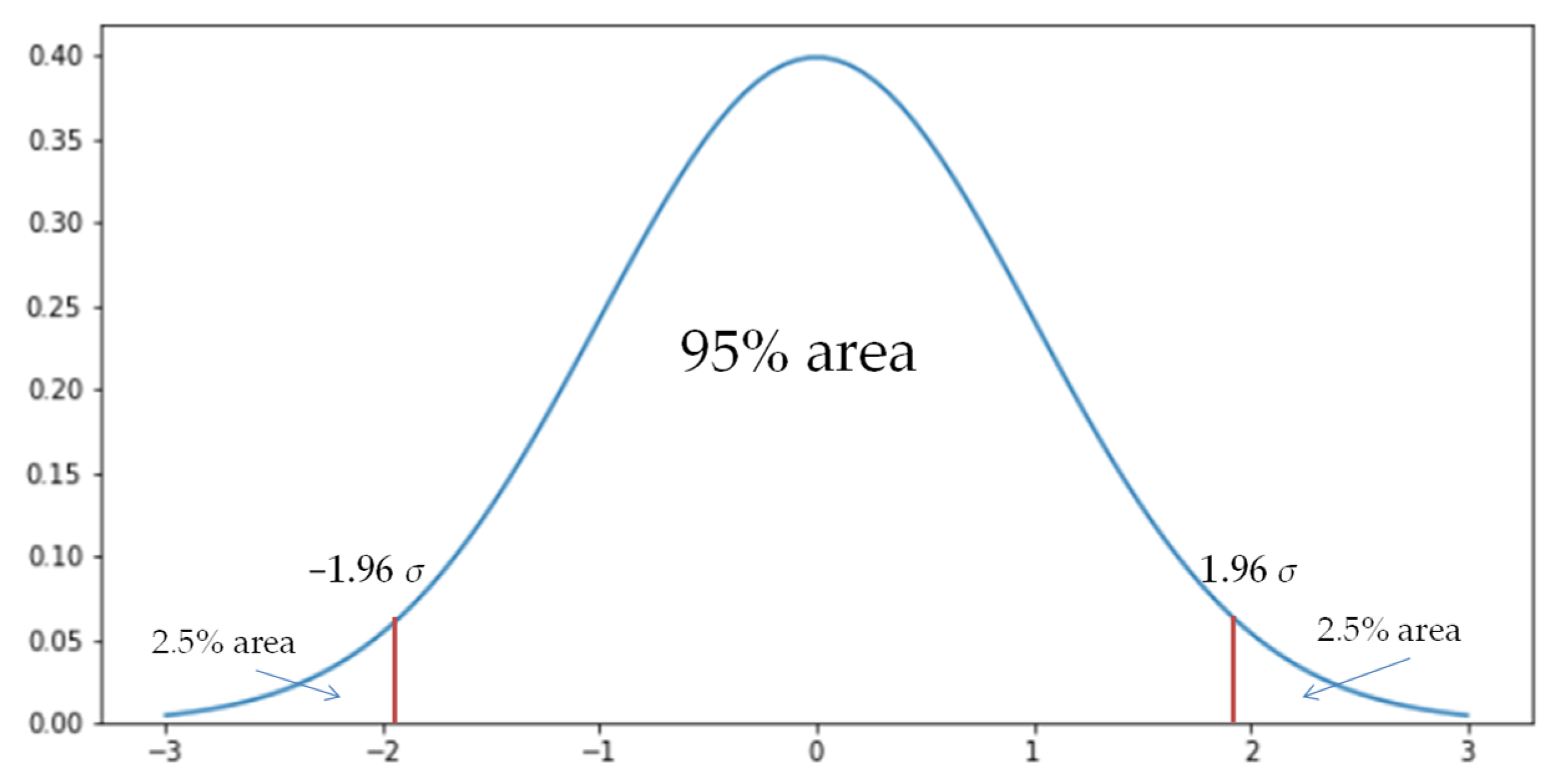
2.3. Confidence Interval (CI) and Confidence Level (CL)
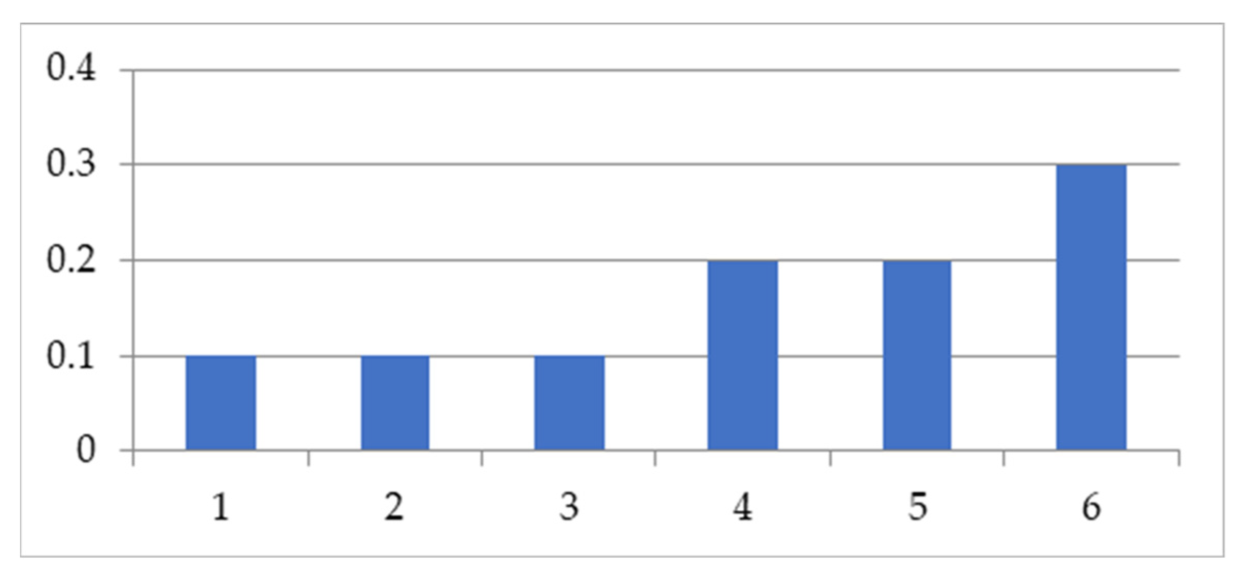
2.4. Discrete Nonuniform Distribution
3. Research Method
3.1. Establishing FMEA Evaluation Model
3.2. Setting CL 95% of Each FMEA Rating
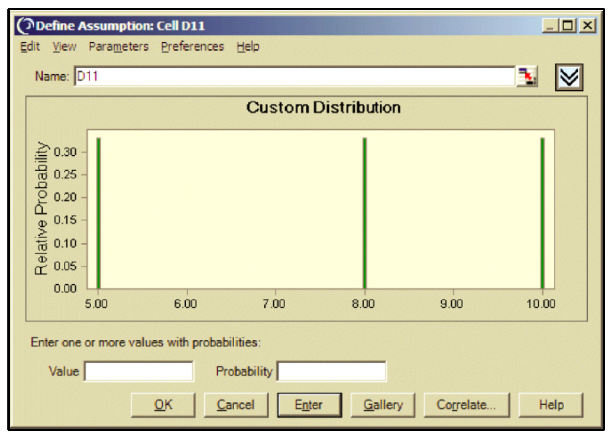
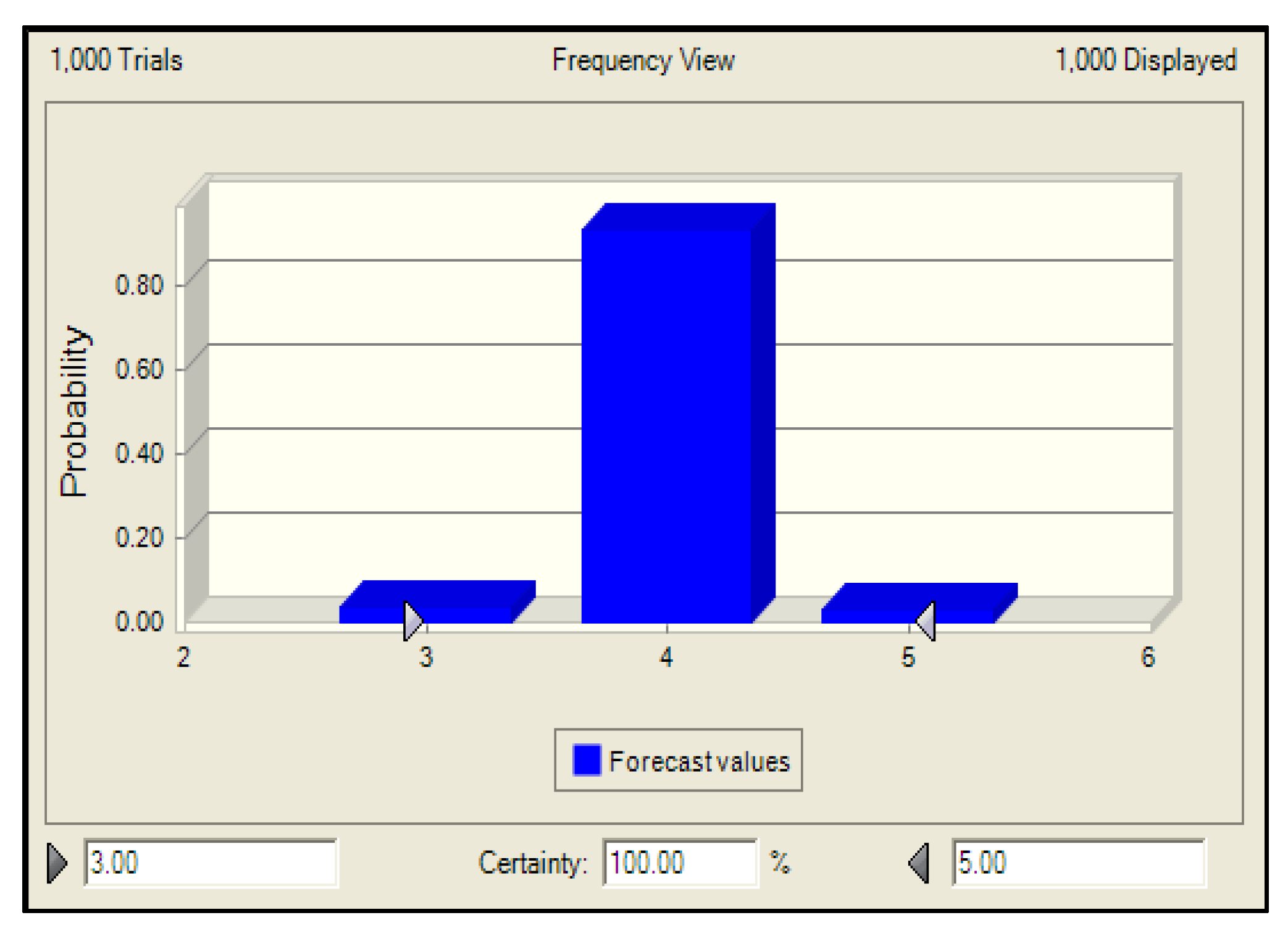
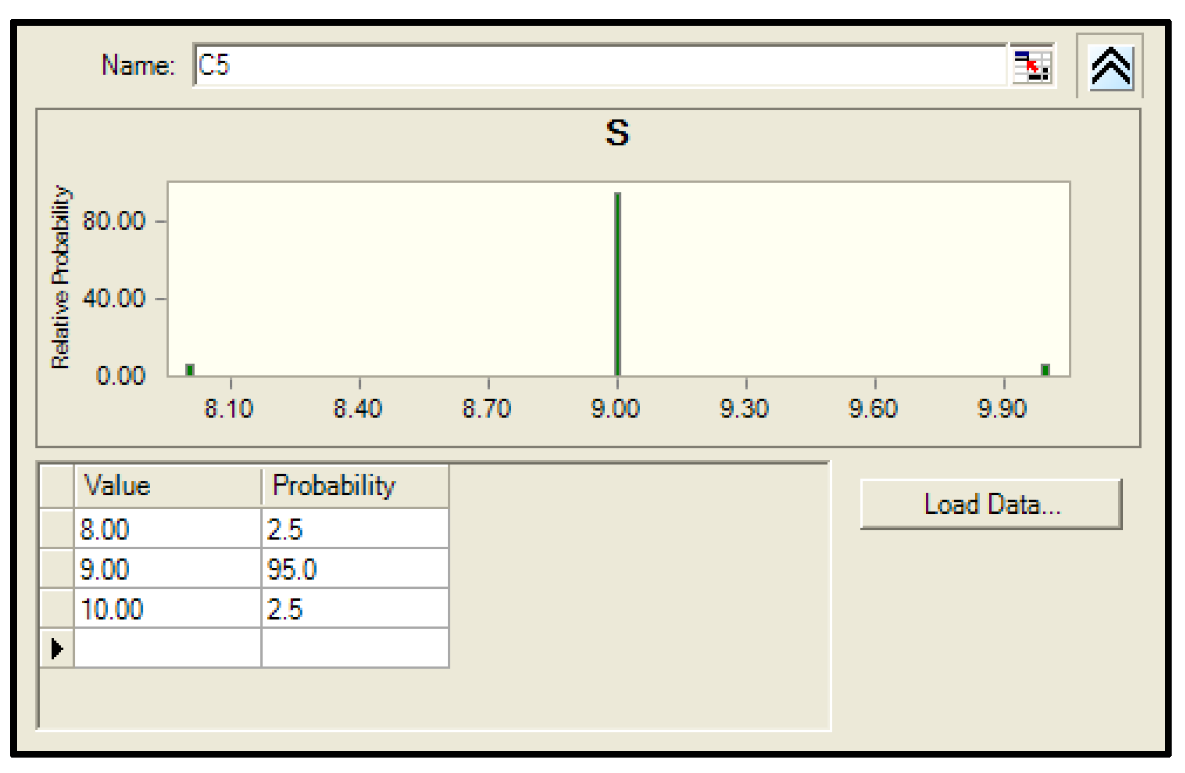
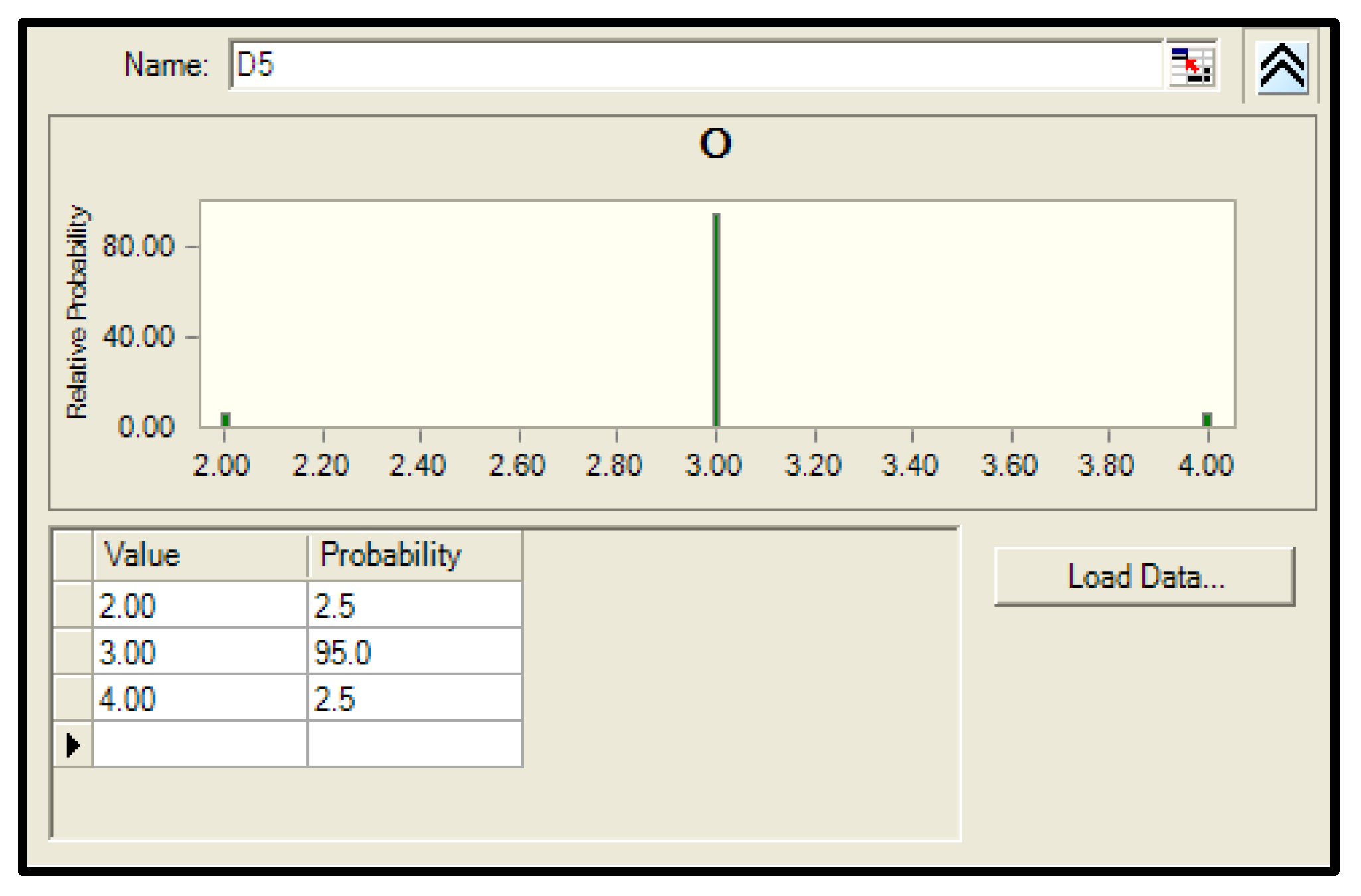
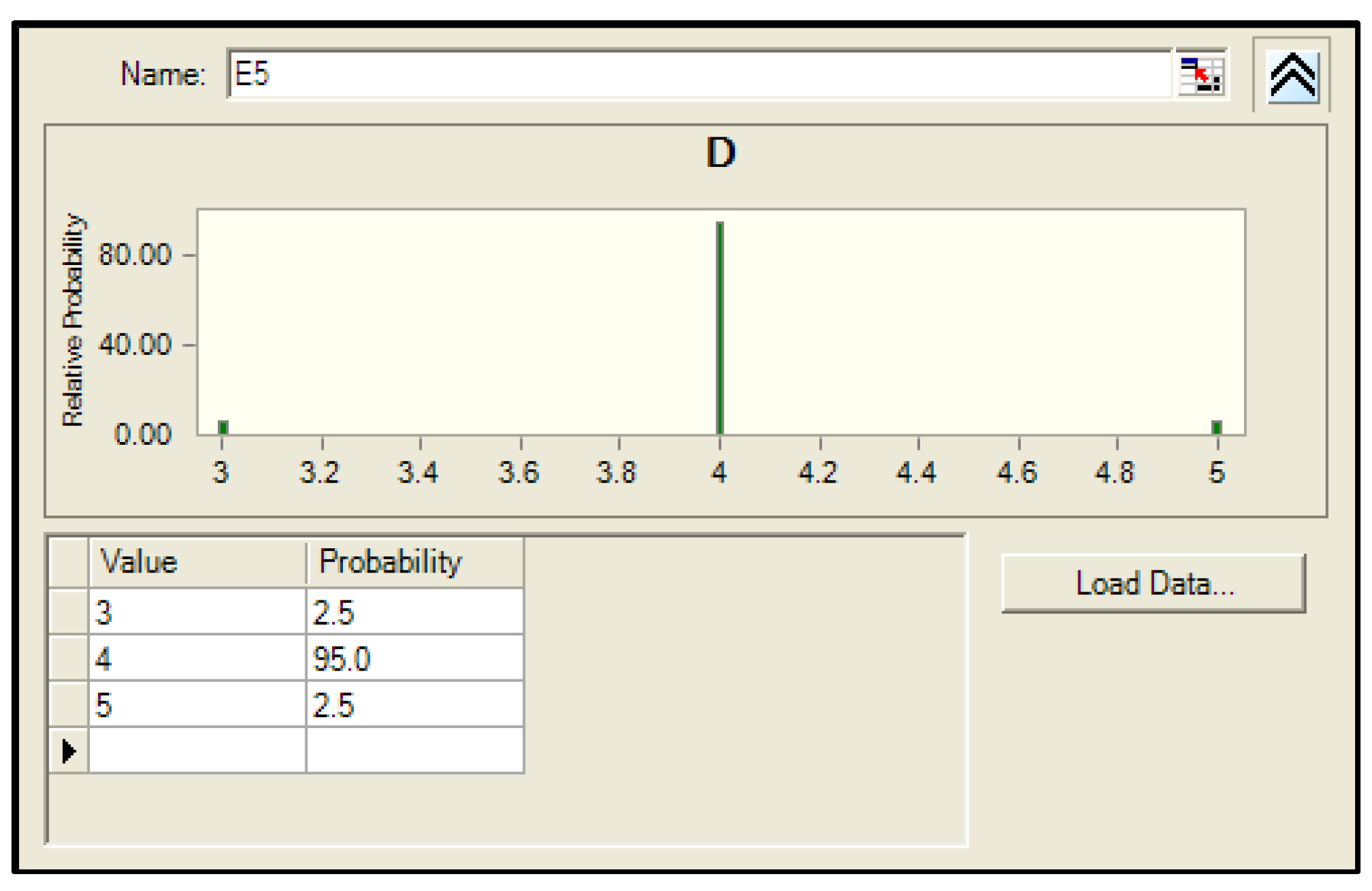
3.3. Setting the Output Model of the Monte Carlo Simulation
3.4. AP Operation Description with the Combination of Monte Carlo Simulation Probability and the Comparison with RPN
4. Research Results
4.1. Data Explanation and Application
- H—
- Highest priority for review and action. The team needs to either identify an appropriate action to improve prevention and/or detection controls or justify and document why current controls are adequate.
- M—
- Medium priority for review and action. The team should identify appropriate actions to improve prevention and/or detection controls, or, at the discretion of the company, justify and document why controls are adequate.
- L—
- Low priority for review and action. The team could identify actions to improve prevention or detection controls.
4.2. Simulation Data for Case 1
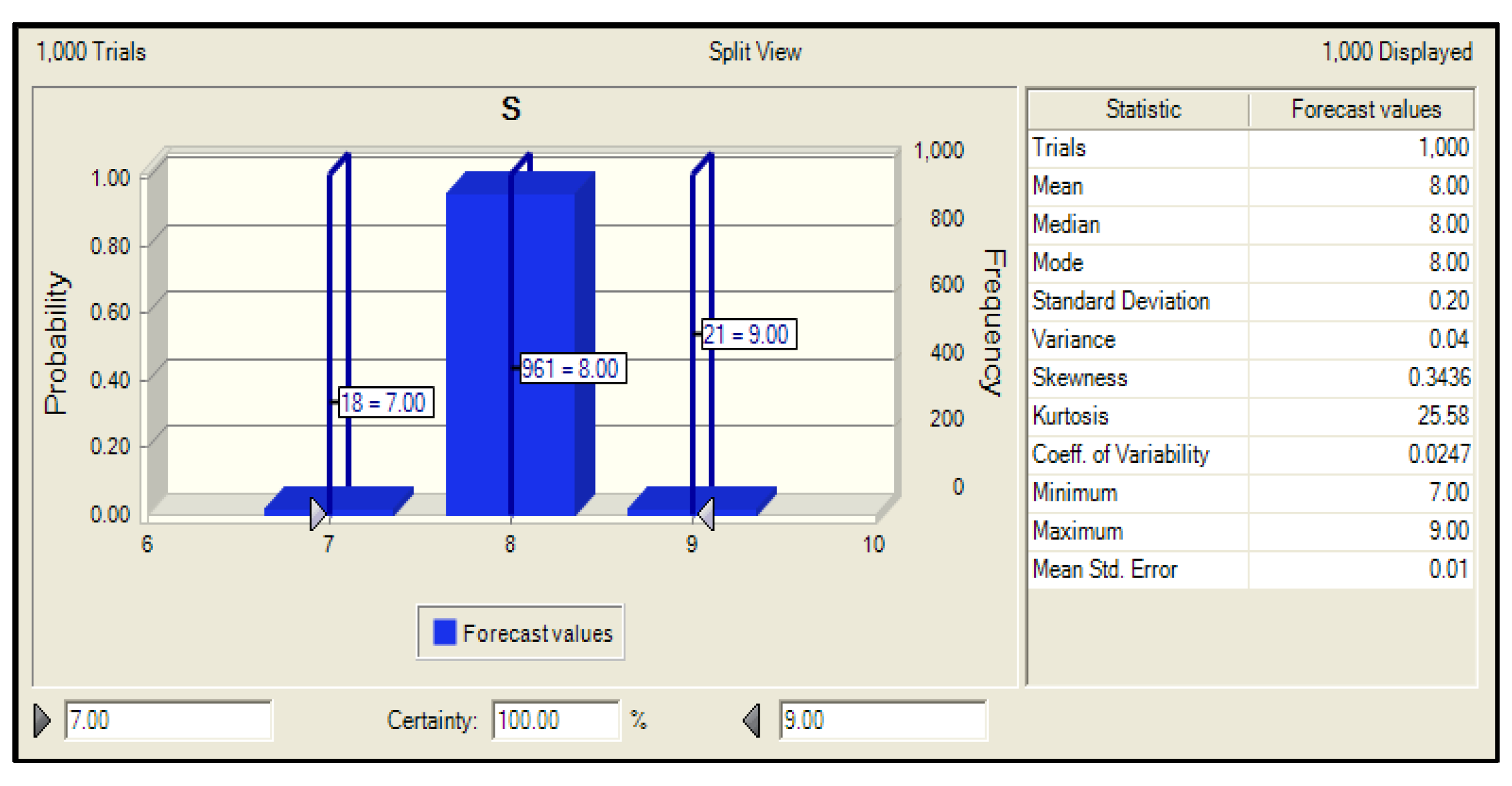
4.3. Analysis Results for Case 1
4.4. Simulation Data for Case 2
4.5. Analysis Results for Case 2
4.6. Discussion
5. Conclusions
Author Contributions
Funding
Institutional Review Board Statement
Informed Consent Statement
Data Availability Statement
Acknowledgments
Conflicts of Interest
References
- Hassan, S.; Wang, J.; Kontovas, C.; Bashir, M. Modified FMEA hazard identification for cross-country petroleum pipeline using Fuzzy rule base and approximate reasoning. J. Loss Prev. Process Ind. 2022, 74, 104616. [Google Scholar] [CrossRef]
- Kapil, D.S.; Shobhit, S. Failure Mode and Effect Analysis (FMEA) implementation: A literature review. J. Adv. Res. Aeronaut. Space Sci. 2018, 5, 1–17. [Google Scholar]
- Gruszka, J.; Misztal, A. The new IATF 16949:2016 standard in the automotive supply chain. Res. Logist. Prod. 2017, 7, 311–318. [Google Scholar] [CrossRef]
- Razouk, H.; Kern, R. Improving the consistency of the Failure Mode Effect Analysis (FMEA) documents in semiconductor manufacturing. Appl. Sci. 2022, 12, 1840. [Google Scholar] [CrossRef]
- Akhyar, Z. A systematic literature review of failure mode and effect analysis (FMEA) implementation in industries. Indones. J. Ind. Eng. Manag. 2020, 2, 59–68. [Google Scholar]
- Tong, L.I.; Wang, C.H.; Chen, H.C. Optimization of multiple responses using principal component analysis and technique for order preference by similarity to ideal solution. Int. J. Adv. Manuf. Technol. 2005, 27, 407–414. [Google Scholar] [CrossRef]
- AIAG; VDA. Failure Mode and Effects Analysis (FMEA Handbook), 1st ed.; Automotive Industry Action Group: Southfield, MI, USA, 2019. [Google Scholar]
- Tang, H.Q.; Duan, X.X. Application of health failure mode and effect analysis in the prevention of pressure sore in spine surgery patient. J. Bengbu Med. Coll. 2015, 40, 1262–1263. [Google Scholar]
- Yang, L.L. Dose FMEA try hard to get rid of RPN constraint? Qual. Mag. 2009, 45, 37–39. [Google Scholar]
- Arend, M.G.; Schäfer, T. Statistical power in two-level models: A tutorial based on Monte Carlo simulation. Psychol. Methods 2019, 24, 1–19. [Google Scholar] [CrossRef]
- Wealer, B.; Bauer, S.; Hirschhausen, C.V.; Kemfert, C.; Göke, L. Investing into third generation nuclear power plants—Review of recent trends and analysis of future investments using Monte Carlo Simulation. Renew. Sustain. Energy Rev. 2021, 143, 110836. [Google Scholar] [CrossRef]
- Yeh, T.M.; Sun, J.J. Using the Monte Carlo simulation methods in gauge repeatability and reproducibility of measurement system analysis. J. Appl. Res. Technol. 2013, 11, 780–796. [Google Scholar] [CrossRef]
- Jaroslav, M. Monte Carlo Simulation Method. In Concise Reliability for Engineers; IntechOpen: London, UK, 2016. [Google Scholar] [CrossRef] [Green Version]
- Hsu, T.G.; Lee, K.W. How to determine a sample size in survey research. J. Taiwan Sport Pedagog. 2013, 8, 89–96. [Google Scholar]
- Subriadi, A.P.; Najwa, N.F. The consistency analysis of failure mode and effect analysis (FMEA) in information technology risk assessment. Heliyon 2020, 6, e03161. [Google Scholar] [CrossRef] [PubMed]
- Ebrahimipour, V.; Rezaie, K.; Shokravi, S. An ontology approach to support FMEA studies. Expert Syst. Appl. 2010, 37, 671–677. [Google Scholar] [CrossRef]
- Ying, H.H.; Zhang, M.; Chen, J. An approach to structuring a technology base. J. Chin. Inst. Ind. Eng. 2007, 24, 42–48. [Google Scholar]
- Lin, C.H.; Chung, G.C. Establishing E-service quality model based on FMEA: An example of 3g mobile-communication industry. Logist. Manag. Rev. 2008, 3, 47–58. [Google Scholar]
- Rezaie, K.; Gereie, A.; Ostadi, B.; Shakhseniaee, M. Safety interval analysis: A risk-based approach to specify low-risk quantities of uncertainty for contractor’s bid proposals. Comput. Ind. Eng. 2008, 56, 152–156. [Google Scholar] [CrossRef]
- AIAG. Potential Failure Mode and Effect Analysis (FMAE), 4th ed.; 2008; Available online: https://www.aiag.org/store/publications/details?ProductCode=FMEA-4 (accessed on 14 March 2022).
- Dariusz, P.; Ewa, G.; Ľuboslav, D. Practical application of the new approach to FMEA method according to AIAG and VDA reference manual. Mech. Eng. Transp. 2021, 23, 325–335. [Google Scholar]
- Xu, K.; Xie, M.; Tang, L.C.; Ho, S.L. Fuzzy assessment of FMEA for engine systems. Reliab. Eng. Syst. Saf. 2002, 75, 17–29. [Google Scholar] [CrossRef]
- Pillay, A.; Wang, J. Modified failure mode and effects analysis using approximate reasoning. Reliab. Eng. Syst. Saf. 2003, 79, 69–85. [Google Scholar] [CrossRef]
- Mohamed, A.; Aminah, R.F. Risk management in the construction industry using combined fuzzy FMEA and Fuzzy AHP. J. Constr. Eng. Manag. 2010, 136, 1028–1036. [Google Scholar]
- Warren, G. Modeling failure modes and effects analysis. Int. J. Qual. Reliab. Manag. 1993, 10, 15–23. [Google Scholar]
- Frunza, G.; Radu Rusu, C.G.; Pop, I.M. Study regarding the application of the FMEA (failure modes and effects analysis) method to improve food safety in food services. Sci. Pap. Ser. D Anim. Sci.—Int. Sess. Sci. Commun. Fac. Anim. Sci. 2020, 63, 360–369. [Google Scholar]
- Anackovski, F.; Kuzmanov, I.; Pasic, R. Action priority in new FMEA as factor for resources management in risk reduction. Int. J. Sci. Eng. Res. 2021, 12, 59–68. [Google Scholar]
- Malvin, H.K.; Paula, A.W. Monte Carlo Methods, 2nd ed.; Wiley: New York, NY, USA; Chichester, UK, 2008. [Google Scholar]
- Zhou, J.; Aghili, N.; Ghaleini, E.N.; Bui, D.T.; Tahir, M.M.; Koopialipoor, M. A Monte Carlo simulation approach for effective assessment of flyrock based on intelligent system of neural network. Eng. Comput. 2020, 36, 713–723. [Google Scholar] [CrossRef]
- Zaroni, J.; Maciel, L.B.; Carvalho, D.B.; Pamplona, E.O. Monte Carlo simulation approach for economic risk analysis of an emergency energy generation system. Energy 2019, 172, 498–508. [Google Scholar] [CrossRef]
- Wittwer, J.W. Monte Carlo Simulation Basics. Vertex42.com. 2004. Available online: https://www.vertex42.com/ExcelArticles/mc/MonteCarloSimulation.html (accessed on 22 March 2022).
- Park, S.K.; Miller, K.W. Random number generators: Good ones are hard to find. Commun. ACM 1988, 31, 1192–1201. [Google Scholar] [CrossRef]
- Lehmer, D.H. Mathematical methods in large-scale computing units. In Proceedings of the Second Symposium on Large Scale Digital Computing Machinery; Harvard University Press: Cambridge, MA, USA, 1951; pp. 141–146. [Google Scholar]
- Gonzalez, A.G.; Herrador, M.A.; Asuero, A.G. Uncertainty evaluation from Monte-Carlo simulations by using Crystal-Ball software. Accredit. Qual. Assur. 2005, 10, 149–154. [Google Scholar] [CrossRef]
- Law, A.M.; Kelton, W.D. Simulation Modeling and Analysis; McGraw-Hill: Boston, MA, USA, 2000. [Google Scholar]
- Eduardo, F.; Gilson, B.; Annibal, P.; Renato, A.; Pedro, M.; Luiz, O. Stochastic risk analysis: Monte Carlo simulation and FMEA (Failure Mode and Effect Analysis). Rev. Espac. 2017, 38, 26. [Google Scholar]
- Seung, J.R.; Kosuk, L. Life cost-based FMEA incorporating data uncertainty. In Proceedings of the ASME 2002 International Design Engineering Technical Conferences and Computers and Information in Engineering Conference, Montreal, QC, Canada, 29 September–2 October 2002; pp. 309–318. [Google Scholar]
- Neyman, J. Outline of a theory of statistical estimation based on the classical theory of probability. R. Soc. 1937, 236, 333–380. [Google Scholar]
- Altman, D. Why we need confidence intervals. World J. Surg. 2005, 29, 554–556. [Google Scholar] [CrossRef] [PubMed] [Green Version]
- Weiss, N.A. Introductory Statistics, 10th ed.; Pearson & Addison Wesley: Boston, MA, USA, 2016. [Google Scholar]
- Hoekstra, R.; Morey, R.; Rouder, J. Robust misinterpretation of confidence intervals. Psychon. Bull. Rev. 2014, 21, 1157–1164. [Google Scholar] [CrossRef] [PubMed]
- Brittany, T.F.; Fabrizio, L.; Alessandro, R.; Larry, W.; Sivaraman, B.; Aarti, S. Confidence sets for persistence diagrams. Ann. Stat. 2014, 42, 2301–2339. [Google Scholar]
- Hazra, A. Using the confidence interval confidently. J. Thorac. Dis. 2017, 9, 4124–4129. [Google Scholar] [CrossRef] [Green Version]
- Glen, S. Confidence Level: What is it? StatisticsHowTo.com: Elementary Statistics for the rest of us! Available online: https://www.statisticshowto.com/confidence-level/ (accessed on 14 March 2022).
- Heumann, C.; Schomaker, M. Introduction to Statistics and Data Analysis; Springer International Publishing: Cham, Switzerland, 2016. [Google Scholar]
- Ary, D.; Jacobs, L.C.; Razavieh, A. Introduction to Research in Education; Harcourt Brace College Publishers: Fort Worth, TX, USA, 1996. [Google Scholar]
- Ian, B. phys420/Ph5_distributions. Available online: https://balitsky.com/teaching/phys420/Ph5_distributions.pdf (accessed on 14 March 2022).
- Cross Validated, Non-Uniform Distribution of p-Values When Simulating Binomial Tests under the Null Hypothesis. Available online: https://stats.stackexchange.com/questions/153249/non-uniform-distribution-of-p-values-when-simulating-binomial-tests-under-the-nu (accessed on 14 March 2022).
- Altman, D.; Machin, D.; Bryant, T.; Gardner, M. Statistics with Confidence: Confidence Intervals and Statistical Guidelines; John Wiley & Sons: Hoboken, NJ, USA, 2013. [Google Scholar]


| S | O | D | AP | S | O | D | AP | S | O | D | AP | S | O | D | AP |
| 9–10 | 8–10 | 7–10 | H | 7–8 | 8–10 | 7–10 | H | 4–6 | 8–10 | 7–10 | H | 2–3 | 8–10 | 7–10 | M |
| 5–6 | H | 5–6 | H | 5–6 | H | 5–6 | M | ||||||||
| 2–4 | H | 2–4 | H | 2–4 | M | 2–4 | L | ||||||||
| 1 | H | 1 | H | 1 | M | 1 | L | ||||||||
| 6–7 | 7–10 | H | 6–7 | 7–10 | H | 6–7 | 7–10 | M | 6–7 | 7–10 | L | ||||
| 5–6 | H | 5–6 | H | 5–6 | M | 5–6 | L | ||||||||
| 2–4 | H | 2–4 | H | 2–4 | M | 2–4 | L | ||||||||
| 1 | H | 1 | M | 1 | L | 1 | L | ||||||||
| 4–5 | 7–10 | H | 4–5 | 7–10 | H | 4–5 | 7–10 | M | 4–5 | 7–10 | L | ||||
| 5–6 | H | 5–6 | M | 5–6 | L | 5–6 | L | ||||||||
| 2–4 | H | 2–4 | M | 2–4 | L | 2–4 | L | ||||||||
| 1 | M | 1 | M | 1 | L | 1 | L | ||||||||
| 2–3 | 7–10 | H | 2–3 | 7–10 | M | 2–3 | 7–10 | L | 2–3 | 7–10 | L | ||||
| 5–6 | M | 5–6 | M | 5–6 | L | 5–6 | L | ||||||||
| 2–4 | L | 2–4 | L | 2–4 | L | 2–4 | L | ||||||||
| 1 | L | 1 | L | 1 | L | 1 | L | ||||||||
| 1 | 1–10 | L | 1 | 1–10 | L | 1 | 1–10 | L | 1 | 1–10 | L | ||||
| 1 | 1–10 | 1–10 | L |
| Equipment Failure Mode and Effects Analysis | |||||||||
| Structure Analysis | FMEA No.: 0001 | ||||||||
| 1. Process Item | 2. Process Step | 3. Process Work Equipment | Key Date: 20XX/3/21 | ||||||
| Semiconductor equipment. | Repairing & Abnormal | Troubleshooting, preventive Maintenance | FMEA Start Date: 20XX/4/1 | ||||||
| Failure Analysis | Cross-Functional Team: Process & Equipment Dept. | ||||||||
| 2. Function of Process Item | 3. Process Step | 4. Process Work Equipment | Process Responsibility: Equipmant Dept. | ||||||
| Key Equipment Assessment | Repairer & Maintenance | Accord to OCAP & recover | |||||||
| Failure Effects(FE) | S | Failure Mode(FM) | Failure cause(FC) | Prevention Controls(PC) of FC | O | Detection Control(DC) of FC or FM | D | AP | |
| 1 | Damage equipment or operator. | 9 | NH4 gas leak | Equipment pipe broken | APC System | 3 | To receive and detect equipment message. | 4 | L |
| 2 | Product reworks 10 pcs. | 4 | Equipment down | Equipment PCB broken | APC system | 5 | Receive and detect equipment message, but cannot auto hold equipment when PCB broken. | 6 | M |
| 3 | Effect production, and lead to shipping. | 3 | Equipment down | Unclear equipment issue | APC system | 4 | 100% receive and detect equipment message, auto hold equipment when abnormal happen. | 2 | L |
| 4 | Customer complains, the issue lead to Yield loss 30%. | 8 | Implant dose abnormal | Implanter broken ,and did not notice | APC system | 2 | It cannot detect until product happen abnormal. | 9 | M |
| 5 | Shipping to customer lead to customer complains, and Yield loss 20%. | 8 | Product over ETCH | Equipment Etch time abnormal | APC System | 6 | Receive and detect equipment message, define control Spec., but cannot auto hold equipment when abnormal. | 2 | H |
| 6 | Slight impact on production line. | 4 | Equipment Arm down | Device arm screw loose | APC system | 5 | Receive device signal value to detect device status. | 6 | L |
| 7 | Customer complains, the issue lead to scrap 10 lots. | 8 | Film thickness insufficient | Target position abnormal | APC system | 4 | Unable to detect and only find the device when the product is abnormal | 7 | H |
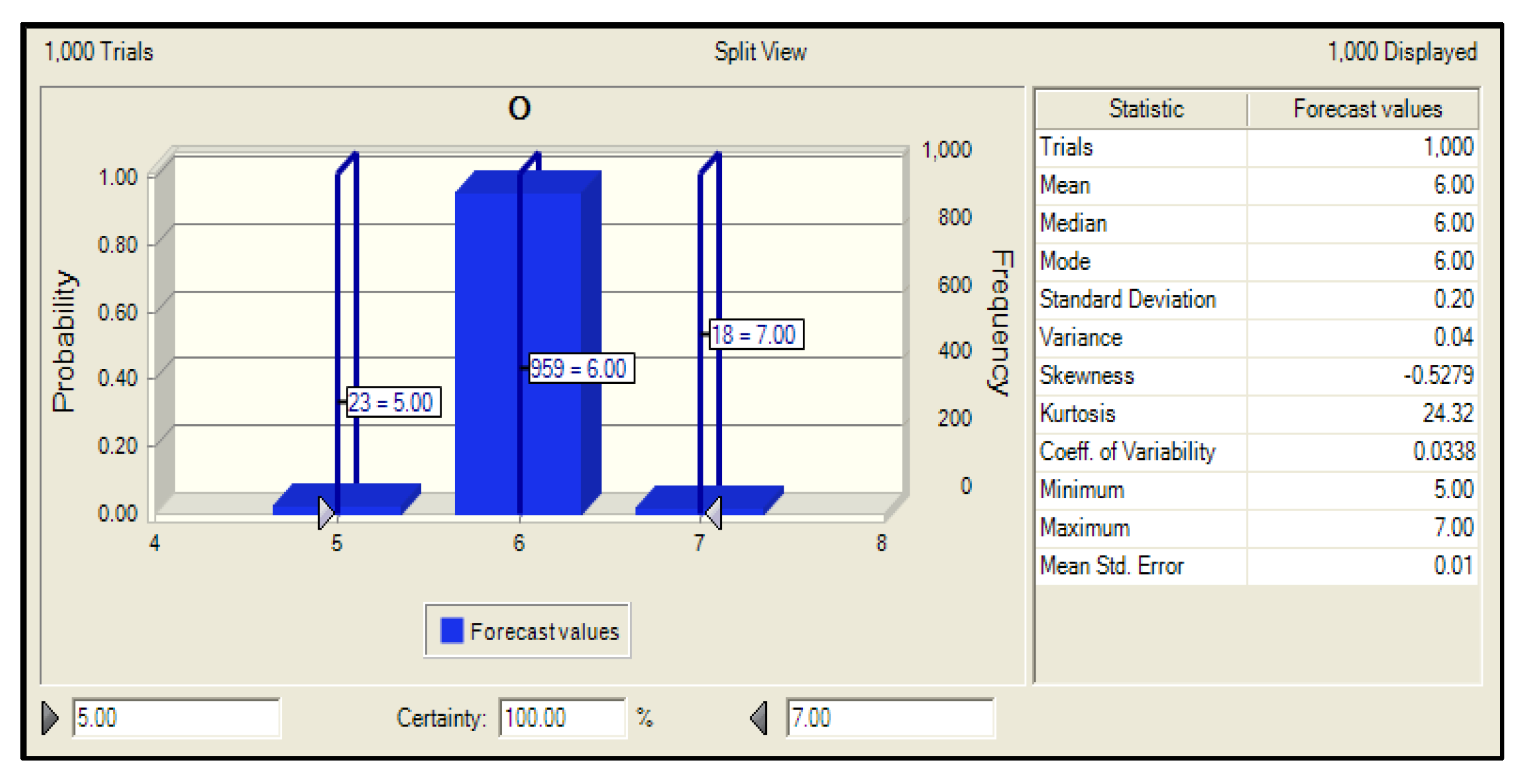
| Severity | Times | Probability | Occurrence | Times | Probability | Detection | Times | Probability |
|---|---|---|---|---|---|---|---|---|
| 9 | 18 | 1.800% | 7 | 23 | 2.300% | 3 | 25 | 2.500% |
| 8 | 961 | 96.100% | 6 | 959 | 95.900% | 2 | 944 | 94.400% |
| 7 | 21 | 2.100% | 5 | 18 | 1.800% | 1 | 31 | 3.100% |
| No. | Severity | Probability | Occurrence | Probability | Detection | Probability | AP | Probability (S * O * D) | RPN |
|---|---|---|---|---|---|---|---|---|---|
| 1 | 9 | 1.800% | 7 | 2.300% | 3 | 2.500% | H | 0.001% | 189 |
| 2 | 9 | 1.800% | 7 | 2.300% | 2 | 94.400% | H | 0.039% | 126 |
| 3 | 9 | 1.800% | 7 | 2.300% | 1 | 3.100% | H | 0.001% | 63 |
| 4 | 9 | 1.800% | 6 | 95.900% | 3 | 2.500% | H | 0.043% | 162 |
| 5 | 9 | 1.800% | 6 | 95.900% | 2 | 94.400% | H | 1.630% | 108 |
| 6 | 9 | 1.800% | 6 | 95.900% | 1 | 3.100% | H | 0.054% | 54 |
| 7 | 9 | 1.800% | 5 | 1.800% | 3 | 2.500% | H | 0.001% | 135 |
| 8 | 9 | 1.800% | 5 | 1.800% | 2 | 94.400% | H | 0.031% | 90 |
| 9 | 9 | 1.800% | 5 | 1.800% | 1 | 3.100% | H | 0.001% | 45 |
| 10 | 8 | 96.100% | 7 | 2.300% | 3 | 2.500% | H | 0.055% | 168 |
| 11 | 8 | 96.100% | 7 | 2.300% | 2 | 94.400% | H | 2.087% | 112 |
| 12 | 8 | 96.100% | 7 | 2.300% | 1 | 3.100% | M | 0.069% | 56 |
| 13 | 8 | 96.100% | 6 | 95.900% | 3 | 2.500% | H | 2.304% | 144 |
| 14 | 8 | 96.100% | 6 | 95.900% | 2 | 94.400% | H | 86.999% | 96 |
| 15 | 8 | 96.100% | 6 | 95.900% | 1 | 3.100% | M | 2.857% | 48 |
| 16 | 8 | 96.100% | 5 | 1.800% | 3 | 2.500% | M | 0.043% | 120 |
| 17 | 8 | 96.100% | 5 | 1.800% | 2 | 94.400% | M | 1.633% | 80 |
| 18 | 8 | 96.100% | 5 | 1.800% | 1 | 3.100% | M | 0.054% | 40 |
| 19 | 7 | 2.100% | 7 | 2.300% | 3 | 2.500% | H | 0.001% | 147 |
| 20 | 7 | 2.100% | 7 | 2.300% | 2 | 94.400% | H | 0.046% | 98 |
| 21 | 7 | 2.100% | 7 | 2.300% | 1 | 3.100% | M | 0.001% | 49 |
| 22 | 7 | 2.100% | 6 | 95.900% | 3 | 2.500% | H | 0.050% | 126 |
| 23 | 7 | 2.100% | 6 | 95.900% | 2 | 94.400% | H | 1.901% | 84 |
| 24 | 7 | 2.100% | 6 | 95.900% | 1 | 3.100% | M | 0.062% | 42 |
| 25 | 7 | 2.100% | 5 | 1.800% | 3 | 2.500% | M | 0.001% | 105 |
| 26 | 7 | 2.100% | 5 | 1.800% | 2 | 94.400% | M | 0.036% | 70 |
| 27 | 7 | 2.100% | 5 | 1.800% | 1 | 3.100% | M | 0.001% | 35 |
| SUM | 100% | ||||||||
| AP | Probability |
|---|---|
| H | 95.243% |
| M | 4.757% |
| L | 0.000% |
| RPN | No. | Probability |
|---|---|---|
| ≧100 | 12 | 44.444% |
| <100 | 15 | 55.556% |
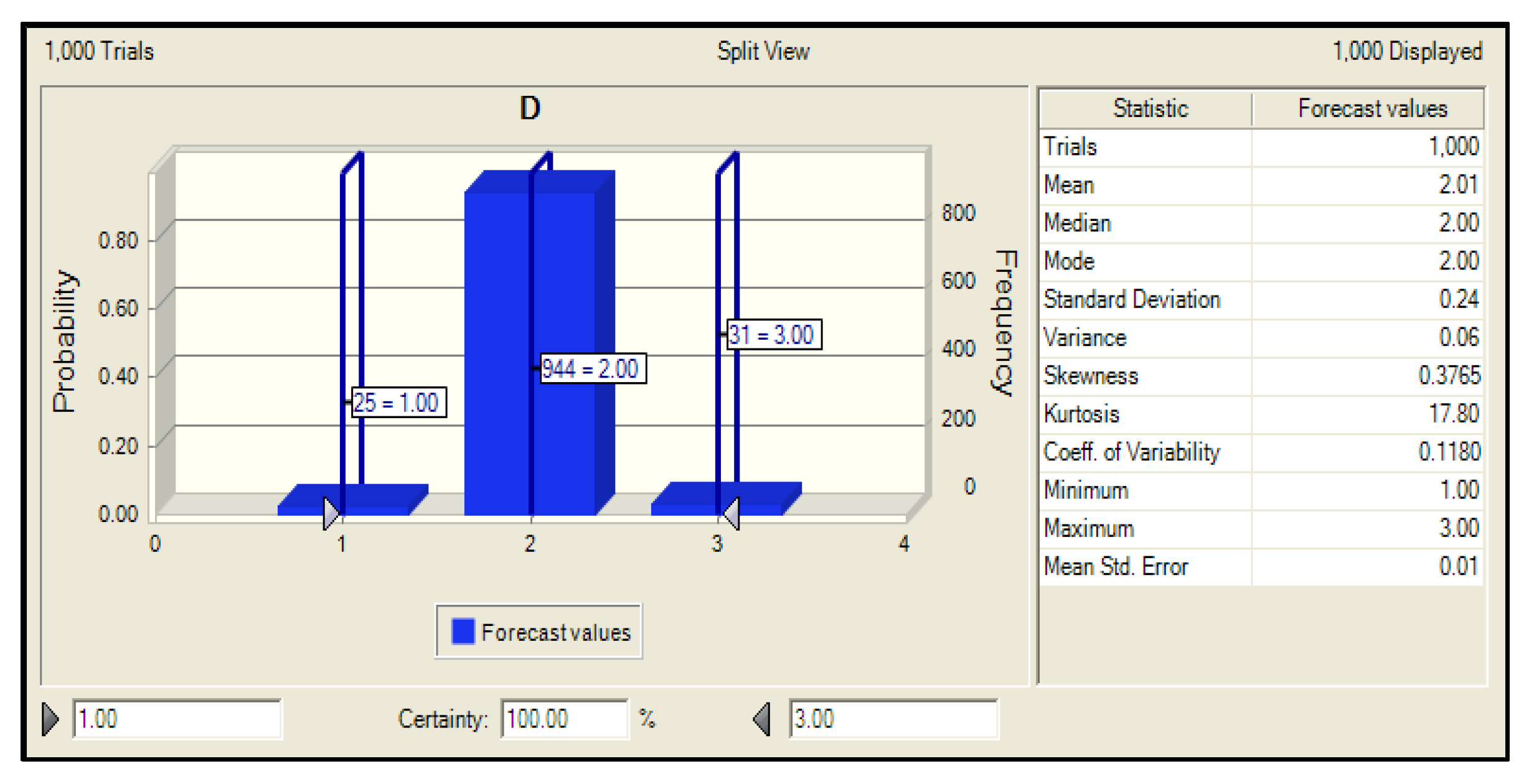
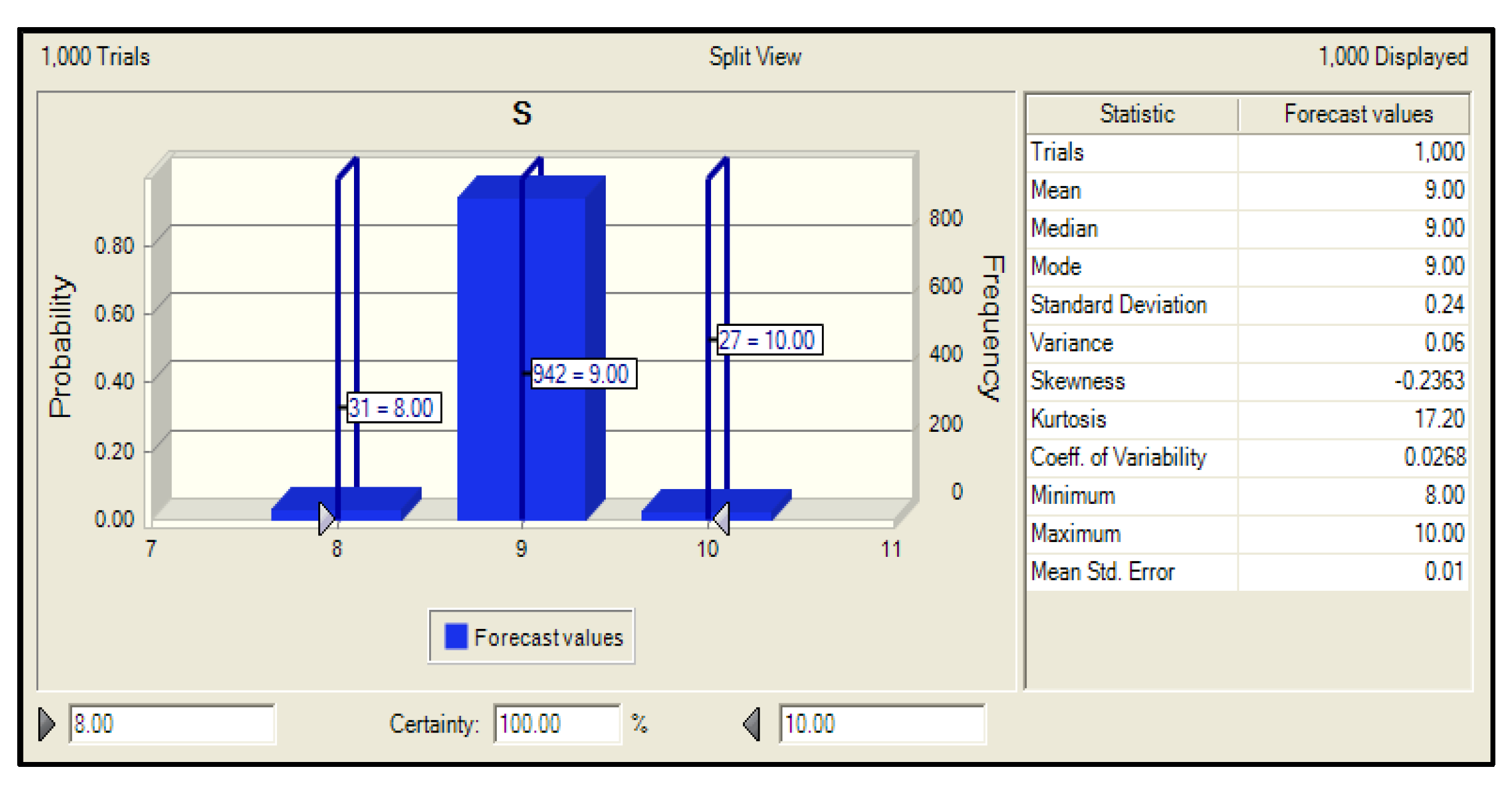
| Severity | Times | Probability | Occurrence | Times | Probability | Detection | Times | Probability |
|---|---|---|---|---|---|---|---|---|
| 10 | 31 | 3.100% | 4 | 24 | 2.400% | 5 | 24 | 2.400% |
| 9 | 942 | 94.200% | 3 | 953 | 95.300% | 4 | 958 | 95.800% |
| 8 | 27 | 2.700% | 2 | 23 | 2.300% | 3 | 18 | 1.800% |
| No. | Severity | Probability | Occurrence | Probability | Detection | Probability | AP | Probability (S * O * D) | RPN |
|---|---|---|---|---|---|---|---|---|---|
| 1 | 10 | 3.100% | 4 | 2.400% | 5 | 2.400% | H | 0.002% | 200 |
| 2 | 10 | 3.100% | 4 | 2.400% | 4 | 95.800% | H | 0.071% | 160 |
| 3 | 10 | 3.100% | 4 | 2.400% | 3 | 1.800% | H | 0.001% | 120 |
| 4 | 10 | 3.100% | 3 | 95.300% | 5 | 2.400% | M | 0.071% | 150 |
| 5 | 10 | 3.100% | 3 | 95.300% | 4 | 95.800% | M | 2.830% | 120 |
| 6 | 10 | 3.100% | 3 | 95.300% | 3 | 1.800% | M | 0.053% | 90 |
| 7 | 10 | 3.100% | 2 | 2.300% | 5 | 2.400% | M | 0.002% | 100 |
| 8 | 10 | 3.100% | 2 | 2.300% | 4 | 95.800% | L | 0.068% | 80 |
| 9 | 10 | 3.100% | 2 | 2.300% | 3 | 1.800% | L | 0.001% | 60 |
| 10 | 9 | 94.200% | 4 | 2.400% | 5 | 2.400% | H | 0.054% | 180 |
| 11 | 9 | 94.200% | 4 | 2.400% | 4 | 95.800% | H | 2.166% | 144 |
| 12 | 9 | 94.200% | 4 | 2.400% | 3 | 1.800% | H | 0.041% | 108 |
| 13 | 9 | 94.200% | 3 | 95.300% | 5 | 2.400% | M | 2.155% | 135 |
| 14 | 9 | 94.200% | 3 | 95.300% | 4 | 95.800% | L | 86.002% | 108 |
| 15 | 9 | 94.200% | 3 | 95.300% | 3 | 1.800% | L | 1.616% | 81 |
| 16 | 9 | 94.200% | 2 | 2.300% | 5 | 2.400% | M | 0.052% | 90 |
| 17 | 9 | 94.200% | 2 | 2.300% | 4 | 95.800% | L | 2.076% | 72 |
| 18 | 9 | 94.200% | 2 | 2.300% | 3 | 1.800% | L | 0.039% | 54 |
| 19 | 8 | 2.700% | 4 | 2.400% | 5 | 2.400% | M | 0.002% | 160 |
| 20 | 8 | 2.700% | 4 | 2.400% | 4 | 95.800% | M | 0.062% | 128 |
| 21 | 8 | 2.700% | 4 | 2.400% | 3 | 1.800% | M | 0.001% | 96 |
| 22 | 8 | 2.700% | 3 | 95.300% | 5 | 2.400% | M | 0.062% | 120 |
| 23 | 8 | 2.700% | 3 | 95.300% | 4 | 95.800% | L | 2.465% | 96 |
| 24 | 8 | 2.700% | 3 | 95.300% | 3 | 1.800% | L | 0.046% | 72 |
| 25 | 8 | 2.700% | 2 | 2.300% | 5 | 2.400% | M | 0.001% | 80 |
| 26 | 8 | 2.700% | 2 | 2.300% | 4 | 95.800% | L | 0.059% | 64 |
| 27 | 8 | 2.700% | 2 | 2.300% | 3 | 1.800% | L | 0.001% | 48 |
| SUM | 100% | ||||||||
| AP | Probability |
|---|---|
| H | 2.335% |
| M | 5.291% |
| L | 92.374% |
| RPN | No. | Probability |
|---|---|---|
| ≧100 | 14 | 51.851% |
| <100 | 13 | 48.149% |
Publisher’s Note: MDPI stays neutral with regard to jurisdictional claims in published maps and institutional affiliations. |
© 2022 by the authors. Licensee MDPI, Basel, Switzerland. This article is an open access article distributed under the terms and conditions of the Creative Commons Attribution (CC BY) license (https://creativecommons.org/licenses/by/4.0/).
Share and Cite
Sun, J.-J.; Yeh, T.-M.; Pai, F.-Y. Application of Monte Carlo Simulation to Study the Probability of Confidence Level under the PFMEA’s Action Priority. Mathematics 2022, 10, 2596. https://doi.org/10.3390/math10152596
Sun J-J, Yeh T-M, Pai F-Y. Application of Monte Carlo Simulation to Study the Probability of Confidence Level under the PFMEA’s Action Priority. Mathematics. 2022; 10(15):2596. https://doi.org/10.3390/math10152596
Chicago/Turabian StyleSun, Jia-Jeng, Tsu-Ming Yeh, and Fan-Yun Pai. 2022. "Application of Monte Carlo Simulation to Study the Probability of Confidence Level under the PFMEA’s Action Priority" Mathematics 10, no. 15: 2596. https://doi.org/10.3390/math10152596