Generalized Accelerated Failure Time Models for Recurrent Events

Abstract

For analyzing recurrent event data, we consider a generalization of the classical accelerated failure time model. In the proposed approach, the general function is no longer assumed to be a singleton but allowed to be time-varying. This is in the same spirit as in quantile regression and the counting process techniques can be utilized. Theoretical properties such as consistency and asymptotic normality are obtained. The illustration of the methodology using simulation studies and then the application to the bladder cancer data is also given.

1. Introduction

Recurrence event data refer to the situation in which events of interest occur repeatedly over time, and these are wildly used in science and technology, especially in medical research, e.g., epileptic seizures, tumor recurrences, or asthma attack. When the investigators studied the recurrent events, they are often interested in the estimation of covariates on recurrent event times, which can help them perform further predictions. The establishment of models can be approached in many ways; meanwhile, the concept of intensity functions and the counting process are also useful. The nonparametric method used to generalize the intensity estimator for the censored failure time data, independently started by [1,2], also denoted the Nelson–Aalen estimator, is one of the methods widely used by investigators. Refs. [3,4], among others, also studied multiplicative models for the rate and mean functions, an approach which can be used with more general models, including regression. Ref. [5] proposed a generalization of the accelerated failure time model, the so-called accelerated recurrence time model, which resembles quantile regression as well as allows for the evolution of covariate effects.

In this paper, we also extend the quantile regression approach and utilize the counting process techniques. For a time-to-event response T, Ref. [6] proposed that a form may assume $Q_T\left(\tau \right|Z)=\exp \left\{X^T{\beta }_0\right\}$ for $\tau \in (0,1)$, where $Q_T\left(\tau \right|Z)=\inf \left\{t:Pr(T\le t|Z)\ge \tau \right\}$, so $Q_T\left(\tau \right|Z)$ can also be seen as the $\tau$-th quantile of T given that the covariates Z and $X={(1,Z^T)}^T$. Here, $T,\tau$ and t denote the time to event, the quantile level, and a non-negative real number, respectively. Since its introduction, quantile regression has been widely used and researched, mainly in survival analysis. Ref. [7] extended the LAD estimation method to more general quantiles, and can also improve efficiency when the error terms are identically distributed. Ref. [5] developed a new quantile regression approach to the counting process, and Ref. [8] adopted a constant general function in quantile regression which it applied to recurrence event data. In the application and algorithm estimation of quantile regression, efforts have also been made by many people. Ref. [9] proposed a locally weighted censored quantile regression approach that can solve covariate-dependent censoring. Ref. [10] proposed a semi-parametric approach using empirical likelihood to a random effects quantile regression model.

Overall, this work considers a situation wherein the general function of the accelerated failure time model is affected by time, sharing the same spirit of the parametric estimation method, while we will use the nonparametric method to estimate the effect. Then, we developed a new counting process model extended from the quantile regression models of this general function. This method provides some ideas for the development of more diverse estimation methods for the counting process.

2. Model

2.1. Accelerated Recurrent Events Time Model

Defining the $R(·)={\sum }_{j=1}^{\infty }I(T^{\left(j\right)}\le ·)$, where $I(·)$ is the indicator function. The observed counting process $N(·)=R(·\wedge L)$ shows that the observation is limited to follow-up time L and ∧ is the minimization operator, meanwhile, the at-risk process $Y(·)$ and $Y\left(t\right)=I(L\ge t)$. We also have ${\mu }_Z=E\left\{R\left(t\right)|Z\right\}$, and Z is a p-vector as the covariates of interest. The original accelerated recurrence time models considered covariates’ effects as time scale changes, which also share the same spirit as quantile regression, and the inverse function is

$${\tau }_Z\left(u\right)=\inf \left\{t:{\mu }_Z\left(t\right)>G\left(u\right)\right\},$$

in a general setting, and $G\left(u\right)=u$ denotes the time to expected frequency u. However, using a constant to estimate the expected frequency has some limitations. For example, the effect of the intervention of interest factors affecting the occurrence of an event may change over time. In this case, the model which combines a constant and variable coefficient may be more effective. As such, we proposed a new accelerated recurrence time model, and the right side of the inequality in the inverse function is $G\left(u\right)=u·m\left(t\right)$ instead of $G\left(u\right)=u$, where $m\left(t\right)$ is the function of time t. Regardless of the form of inverse function, it can be written in the following form:

$$\log {\tau }_Z\left(u\right)=X^T{\beta }_0\left(u\right)$$

(1)

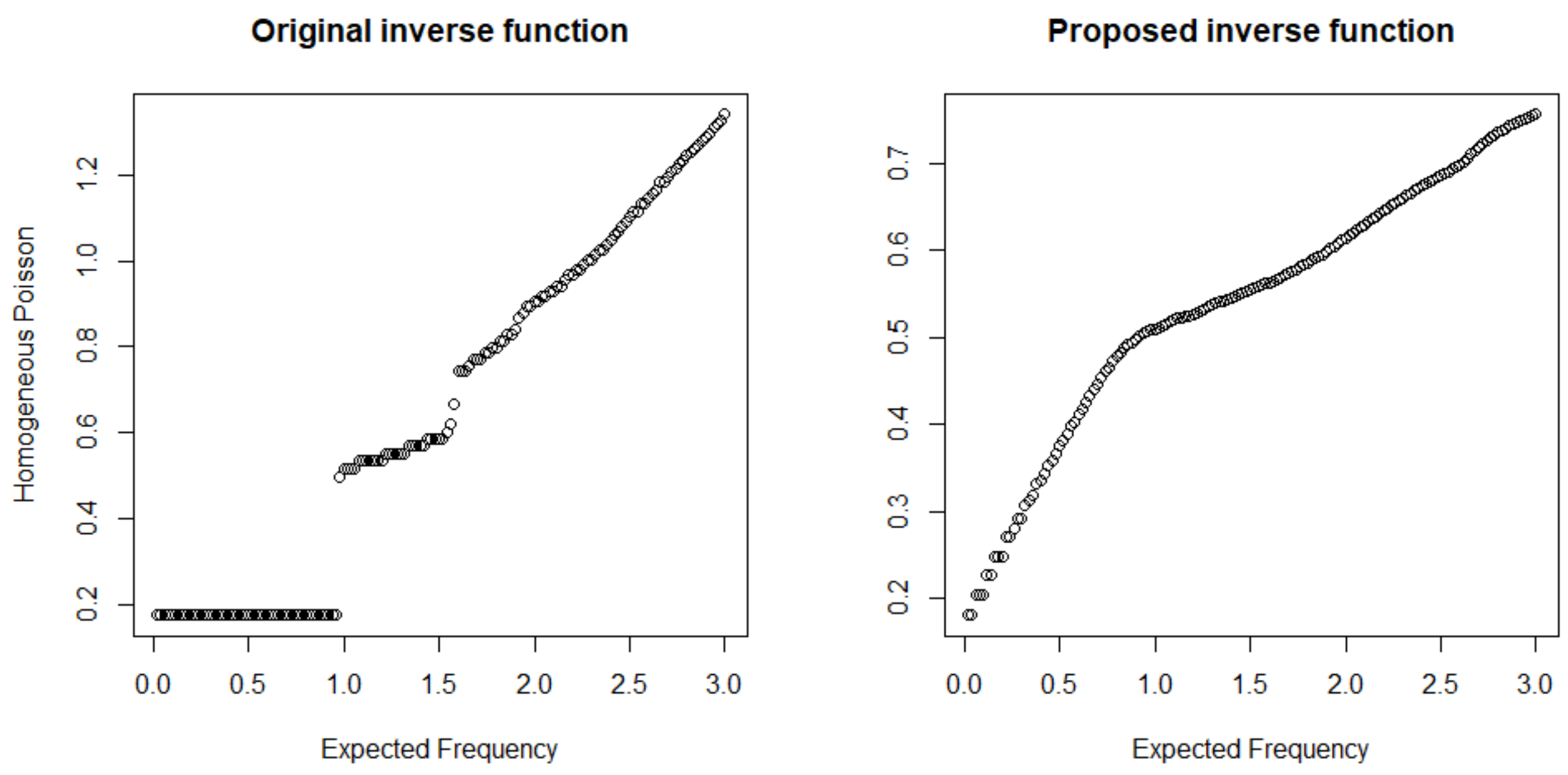
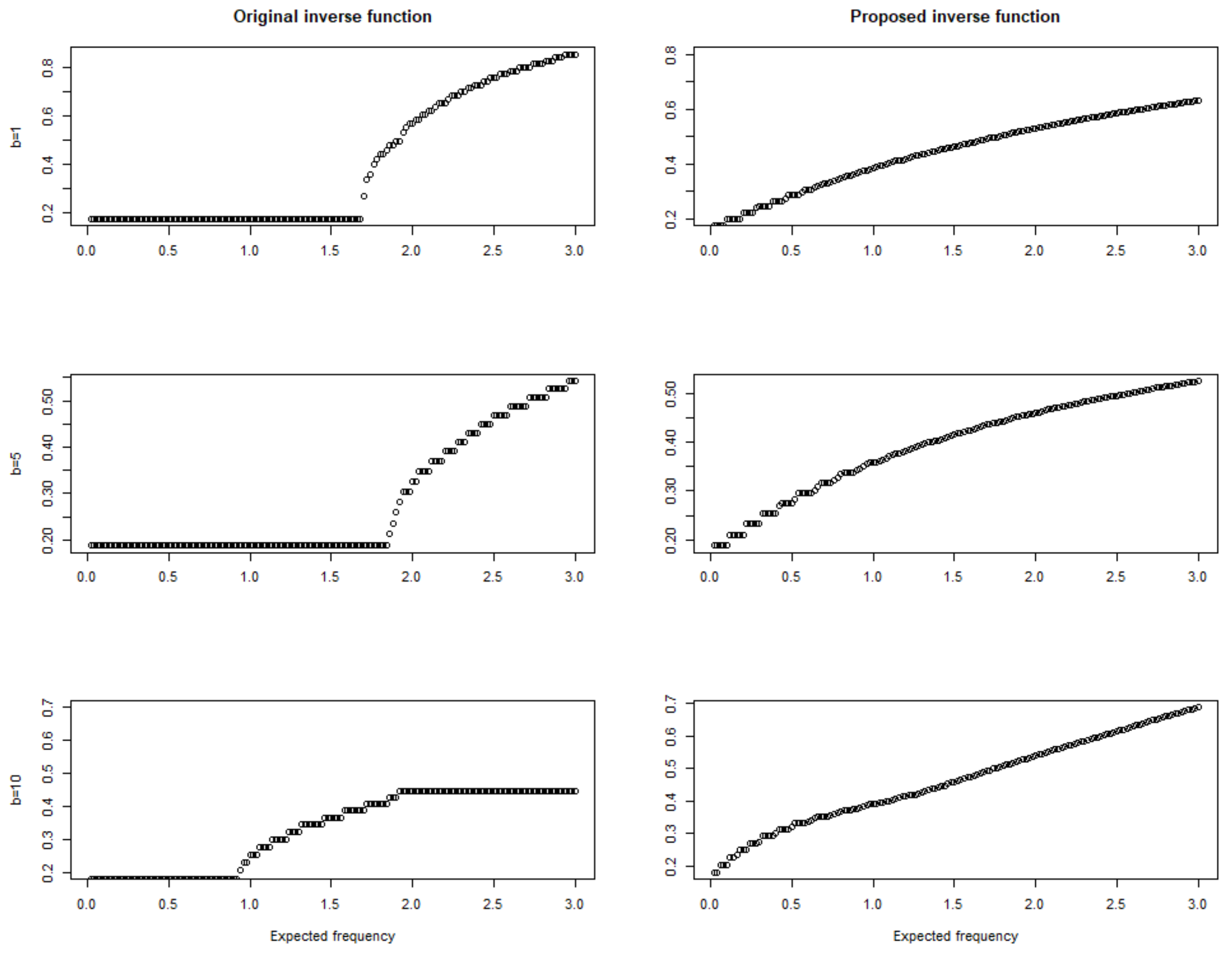
As can be seen from the above formula, $\log {\tau }_Z\left(u\right)$ should be linear. Compared to the original accelerated recurrence model and the improved model, when the recurrent event T follows a homogeneous Poisson distribution, as shown in Figure 1, the estimated log${\tau }_Z\left(u\right)$ by both models is approximately linear when the recurrent event is a non-homogeneous Poisson process, which has an intensity function ${\lambda }_0\left(t\right)$ related to time t. In Figure 2, we compare three different situations, namely when ${\lambda }_0\left(t\right)=b\times t$ and $b=1,5,10$. As b increases, the estimation of the original accelerated recurrence model tends to be more and more nonlinear, while the proposed improved model still shows a strong linear relationship. In that way, the proposed recurrent event time model can be used in a more general situation.

In this paper, we consider the situation that $G\left(u\right)=ut$, then model 2 can be rewritten as

$$E\left(X\left[R\left\{\exp \left(X^T\beta \right)\right\}-\exp \left(X^T\beta \right)u\right]\right)=0$$

(2)

if and only if $\beta ={\beta }_0\left(u\right)$, and the left-hand side should be monotone, then the above equation can be transformed into

$${\beta }_0\left(u\right)=\underset{\beta }{\mathrm{argmin}}E\left\{\sum _{j=1}^{\infty }{(X^T\beta -\log T^{\left(j\right)})}^{+}-\exp \left(X^T\beta \right)u\right\}.$$

where $a^{+}=a\vee 0$ and ∨ denotes the maximization operator. Then, we can come up with the following theorem:

Theorem 1.

For $G\left(u\right)=\exp \left(X^T\beta \left(u\right)\right)u$, if (1) hold and $R\left\{{\tau }_Z\left(u\right)\right\}\perp L\mid Z$, define $v^{⨂2}=v{v}^T$ for vector v, ${\dot{\mu }}_Z(·)$ is the derivative of ${\mu }_Z$, let $F_Z\left(x\right)=E\left\{Y\left(x\right)\mid Z\right\}$, and assume

(C1) 

$E\left[X^{⨂2}I\left\{L>{\tau }_Z\left(u\right)\right\}\right]$ is non-singular;

(C2) 

${\dot{\mu }}_Z\left(e^{X^T{\beta }_0\left(u\right)}\right)F_Z\left(e^{X^T{\beta }_0\left(u\right)}\right)>U$ for all $u\in (0,U]$.

Then,

$${\beta }_0\left(u\right)=\underset{\beta }{\mathrm{argmin}}\psi (\beta ;u),$$

(3)

where

$$\psi (\beta ;u)=E\left\{\sum _{j=1}^M{(X^T\beta \wedge \log L-\log T^{\left(j\right)})}^{+}-\exp (X^T\beta \wedge \log L)u\right\}.$$

The proof of this result, as well as the proofs for Theorems 2 and 3 below, are given in Appendix A. Powell extended these results for censored quantile regression when the censoring time is observed [7]. We will then combine the counting process model and apply this method to the recurrence events data.

2.2. The Recurrent Events Model

For the counting process model, we begin with a review of Gill and Andersen’s study [11], which extended the Cox proportional hazards model [12] to a multivariate counting process. The intimate connection of the study on the multivariate counting process and the use of martingale methods can allow us to derive more properties of the statistical estimation and testing procedures. As each component $N_i(·)$ of a multivariate counting process has a cumulative hazard function ${\mathsf{\Lambda }}_T(·)$, there exist local martingales $M_i$ defined by $M_i\left(t\right)=N_i\left(t\right)-{\mathsf{\Lambda }}_T\left(t\right)$. Since the cumulative hazard function ${\mathsf{\Lambda }}_T(·)$ is the integral of the hazard function, then according to [11], the counting process formation of the Cox model can be given by

$$E\left\{N\left(t\right)\mid Z\right\}=E\left\{{\int }_0^{u}Y\left(s\right){\lambda }_0\left(s\right)e^{X^{T}b}ds\mid Z\right\},t>0,$$

(4)

where ${\lambda }_0\left(s\right)$ denotes the baseline hazard function, and this model can accommodate recurrent events data well. Peng and Huang conducted a re-examination work [5], which combined the quantile regression method for survival data with the above counting process model.

$$E\left\{N\left(e^{X^T{\beta }_0\left(u\right)}\right)\mid Z\right\}=E\left\{{\int }_0^{u}Y\left(e^{X^T{\beta }_0\left(s\right)}\right)\frac{1}{1-s}ds\mid Z\right\},u\in (0,1),$$

(5)

which has a nice monotonicity property. In model 6, the estimated cumulative hazard function ${\widehat{\mathsf{\Lambda }}}_T\left(x\right)=-\log (1-x)$. Huang also showed that a singleton model, where an estimated cumulative hazard function is a constant u, can also be applied in the counting process model [13]. When the singleton model is combined with quantile regression, this extended the following model to a more general situation of recurrent events [8], and the estimation formula is given by

$$E\left\{N\left(e^{X^T{\beta }_0\left(u\right)}\right)\mid Z\right\}=E\left\{{\int }_0^{u}Y\left(e^{X^T{\beta }_0\left(s\right)}\right)g\left(s\right)ds\mid Z\right\},u\in (0,1),$$

(6)

where $g\left(s\right)\equiv 1$. In fact, in model 7, the estimated cumulative hazard function $G\left(u\right)=u$, which is a constant. According to Theorem 1 and the above models, we can propose a new counting process model that takes the form

$$E\left\{N\left(e^{X^T{\beta }_0\left(u\right)}\right)\mid Z\right\}=E\left\{{\int }_0^{u}Y\left(e^{X^T{\beta }_0\left(s\right)}\right)dG\left(s\right)\mid Z\right\},u\in (0,U],$$

(7)

where in our model, we can also show that

$${\mu }_Z\left(e^{X^T{\beta }_0\left(u\right)}\right)=G\left(u\right)=ut={\int }_0^{u}g\left(s\right)ds.$$

Therefore, we also have an alternative representation of the model that

$${\tau }_Z\left(G\left(u\right)\right)=\exp \left\{X^T{\beta }_0\left(u\right)\right\},u\in (0,U],$$

(8)

The proof of this recurrence events setting is also shown in the Appendix A. In the simulation part, we will show that our estimation method performs better when the recurrent event time follows the non-homogeneous Poisson distribution.

2.3. The Proposed Estimation Procedure

From Theorem 1, we can define the objective function

$$\mathsf{\Psi }(\beta ;u)=n^{-1}\sum _{i=1}^n\left\{\sum _{j=1}^{M_i}{(X_i^T\beta \wedge \log L_i-\log T_i^{\left(j\right)})}^{+}-\exp (X_i^T\beta \wedge \log L_i)u)\right\}.$$

(9)

Theorem 1 leads to the estimation of ${\beta }_0\left(u\right)$, that is $\widehat{\beta }\left(u\right)=\underset{\beta }{\mathrm{argmin}}\mathsf{\Psi }(\beta ;u)$.

It can be seen that the objective function is not convex. An algorithm was developed to find the local minimizer that is asymptotically equivalent to the global minimizer [13]. Since we proposed the counting process-based model (model 7), then we can propose an equation to estimate ${\beta }_0\left(u\right)$:

$$n^{1/2}{S}_n(\beta ,u),$$

(10)

where

$$S_n(\beta ,u)=n^{-1}\sum _{i=1}^n{X}_i\left\{N_i\left(\exp \left\{X_i^T\beta \left(u\right)\right\}\right)-{\int }_0^{u}I(L_i\ge \exp \left\{X_i^T\beta \left(s\right)\right\})dG\left(s\right)\right\}.$$

As the results proposed in [11], although $M_h$ is a local square integrable martingale, it has the same asymptotic property as a global martingale, and if we let $S(\beta ,u)=E\left\{S_n(\beta ,u)\right\}$, then follows the martingale property of $M(·)$ given that $S({\beta }_0,u)=0$.

Equation (8) boils down to the estimation of censored quantile regression in [5]. A common method used to predict ${\beta }_0\left(u\right)$ is the grid-based estimation procedure by denoting ${\beta }_0\left(u\right)$ as a right-continuous piecewise-constant function that jumps on a grid. More specifically, we define $S_{L\left(n\right)}=\left\{0=u_0<u_1<\cdots <u_{L\left(n\right)}=U\right\}$, and for our recurrence setting, the U in the grid can be greater than 1. The size of $S_{L\left(n\right)}$, denoted by $∥S_{L\left(n\right)}∥$, is the maximum value of $u_j-u_{j-1}$ where $j=1,\cdots ,L\left(n\right)$. It is also noteworthy that $\exp \left\{X^T\widehat{\beta }\left(0\right)\right\}=0$. Thus, based on model 9, we can estimate $\widehat{\beta }\left(u_j\right)$ by sequentially solving the estimating equation

$$n^{-1/2}\sum _{i=1}^n{X}_i\left\{R_i\left(\exp \left\{X_i^T\beta \left(u_j\right)\right\}\right)-\sum _{k=0}^{j-1}I(L_i\ge \exp \left\{X_i^T\widehat{\beta }\left(u_k\right)\right\}){\int }_{u_k}^{u_{k+1}}g\left(s\right)ds\right\}=0,$$

(11)

Since Equation (10) is not continuous, the exact root may not exist. Fygenson and Ritov proposed a generalization solution of $\widehat{\beta }\left(u_j\right)$ for monotone estimating equations [14]. To find the generalization solution of Equation (10), we need to perform some simple algebraic manipulations, and then the solution-finding problem is equivalent to locating the minimizer of the following $L_1$-type convex function:

$$\begin{array}{cc}\hfill l_j\left(h\right)& =\sum _{i=1}^n\sum _{j=1}^{\infty }I(T_i^{\left(j\right)}\le L_i)\left|\log T_i^{\left(j\right)}-X_i^{T}h\right|+\left|R^{\ast }-\left\{\sum _{i=1}^n\sum _{j=1}^{\infty }I(T_i^{\left(j\right)}\le L_i){(-X_i)}^{T}h\right\}\right|\hfill \\ \hfill & +\left|R^{\ast }-\left\{\sum _{i=1}^{n}2X_i^{T}h\sum _{k=0}^{j-1}I(L_i\ge \exp \left\{X_i^T\widehat{\beta }\left(u_k\right)\right\})\exp \left\{X_i^T\widehat{\beta }\left(u_k\right)\right\}(u_{k+1}-u_k)\right\}\right|.\hfill \end{array}$$

where $R^{\ast }$ is a very large number and $j=1,\cdots ,L\left(n\right)$. One can also solve the $l_j\left(h\right)$ by using statistical software, such as the $\mathit{rq}\left(\right)$ function in R package $\mathit{quantreg}$ or the $\mathit{l}\mathit{1}\mathit{fit}\left(\right)$ function in S-PLUS.

2.4. Asymptotic Properties

In this section, we establish the uniform consistency and weak convergence of the proposed estimator $\widehat{\beta }\left(u\right)$. Firstly, some regularity conditions should be stated.

Define $\mu \left(b\right)=E\left\{XN\left(\exp \left(X^{T}b\right)\right)\right\}$, $\tilde{\mu }\left(b\right)=E\left\{XI(\exp \left(X^{T}b\right)\le L)\right\}$, ${\tilde{\mu }}_Z\left(x\right)=E\left(N\right(x\left)\right|Z)$, $g_Z\left(x\right)=d{\tilde{\mu }}_Z\left(x\right)/dx$, $F\left(t\right|Z)=Pr(x\le t\left|Z\right)$, $\overline{f}\left(x\right|Z)=-f\left(x\right|Z)=-dF\left(x\right|Z)/dx$. By using simple algebra, we also define $B\left(b\right)=d\mu \left(b\right)/d{b}^T=E\left\{X^{⨂2}{e}^{X^{T}b}{g}_Z\left(e^{X^{T}b}\right)\right\}$, $J\left(b\right)=d\tilde{\mu }\left(b\right)/d{b}^T=E\left\{X^{⨂2}{e}^{X^{T}b}\overline{f}\left(e^{X^{T}b}\right|Z)\right\}$. Suppose the assumptions in Theorem 1 hold and $\widehat{\beta }\left(u\right)$ is strongly consistent for ${\beta }_0\left(u\right)$. Assume the following conditions:

(C1’)

Z and $N\left(L\right)$ are bounded;

(C2’)

(a) ${\dot{\mu }}_Z(·)$ is bounded and continuous at $t={\tau }_Z\left(u\right)$, as well as uniform in Z, and (b) $\mu \left({\beta }_0\left(u\right)\right)$ is a Lipschitz function of u;

(C3’)

(a) each component of $J\left(b\right)B{\left(b\right)}^{-1}$ is uniformly bound on $b\in \mathcal{B}\left(d\right)$, where $\mathcal{B}\left(d\right)$ is a neighborhood containing ${\beta }_0\left(u\right)$, (b) $g_Z\left(x\right)>0$ and $E\left(Z^{⨂2}\right)$ is positive definite;

(C4’)

${\inf }_{u\in [v,U]}\mathrm{eigmin}B\left({\beta }_0\left(u\right)\right)>0$ for any $v\in (0,U]$, where $\mathrm{eigmin}(·)$ denotes the minimum eigenvalue of a matrix.

Condition (C1’) implies the boundedness of covariates and the number of observed events, and (C2’) gives the smoothness of ${\beta }_0\left(u\right)$, condition (C3’) sets additional mild assumptions such as the positive definite. Noted that (C4’) is a key condition that ensures the consistency of the proposed estimator. Then, we have the following theorems.

Theorem 2.

Under conditions C1’–C4’, when ${lim}_{n\to \infty }∥S_{L\left(n\right)}∥=0$, then

$$\underset{u\in (v,U]}{\sup }∥\widehat{\beta }\left(u\right)-{\beta }_0\left(u\right)∥\stackrel{P}{\to }0,$$

where $0<v<U$.

Theorem 3.

Under condition C1’–C4’, when ${lim}_{n\to \infty }{n}^{1/2}∥S_{L\left(n\right)}∥=0$, then

$$n^{1/2}\left\{\widehat{\beta }\left(u\right)-{\beta }_0\left(u\right)\right\}$$

converge weakly to a Gaussian process for $u\in [v,U]$, where $v\in (0,U)$.

The proofs are also in the Appendix A.

3. Simulation Studies

In this part, we conducted the Monte Carlo simulations to test our model. Combining the methods of Huang and Peng [13], recurrent events were generated from both homogeneous Poisson and non-homogeneous Poisson processes. We also generated two covariates, $X_1$ and $X_2$, following the distribution $Bernoulli\left(0.5\right)$ and $Unif(-0.5,0.5)$ separately. The recurrent event time was generated by:

$$T^{\left(j\right)}=\exp \left\{\min (1,\frac{T^{\ast \left(j\right)}}{1.5\gamma })X_1+X_2\right\}{T}^{\ast \left(j\right)}/\gamma ,j=1,2,...,$$

where in one case, $\left\{T^{\ast \left(j\right)},j=1,2,\dots \right\}$ was a recurrent event time from the standard homogeneous Poisson process, in other words, the gap times of $T^{\ast \left(j\right)}-T^{\ast (j-1)}$ are independent and identically $exponetial\left(1\right)$ variables; in other cases, $\left\{T^{\ast \left(j\right)},j=1,2,...\right\}$ is a recurrent event time from the non-homogeneous Poisson process with the intensity function ${\lambda }_0\left(t\right)=t$. Furthermore, the frailty $\gamma$ followed the Gamma distribution for the homogeneous Poisson process, we considered two situations, that is the variance of $\gamma$ was chosen to be 0 and 0.5, for the non-homogeneous Poisson process, and we only consider the variance of $\gamma$ to be 0. Under our simulation setup, we have

$${\tau }_Z\left(G\left(u\right)\right)=\exp \left\{\log \left(u\right)+\min (1,u/1.5)X_1+X_2\right\}.$$

For censoring time L, we generated it from $Unif(0,12)$. For each selection of the variance of $\gamma$, we generated 500 datasets of sample size $n=100$. Since we adopted the grid-based method to estimate the $\beta$, an equally spaced grid on $u\in (0,3]$ with step size 0.02 was conducted in our simulation.

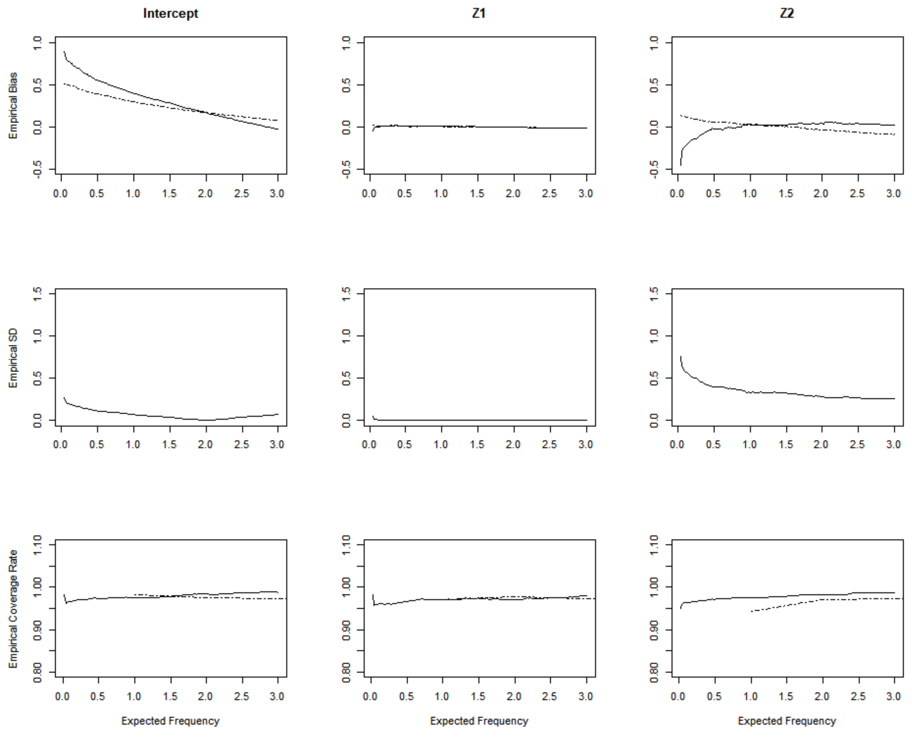
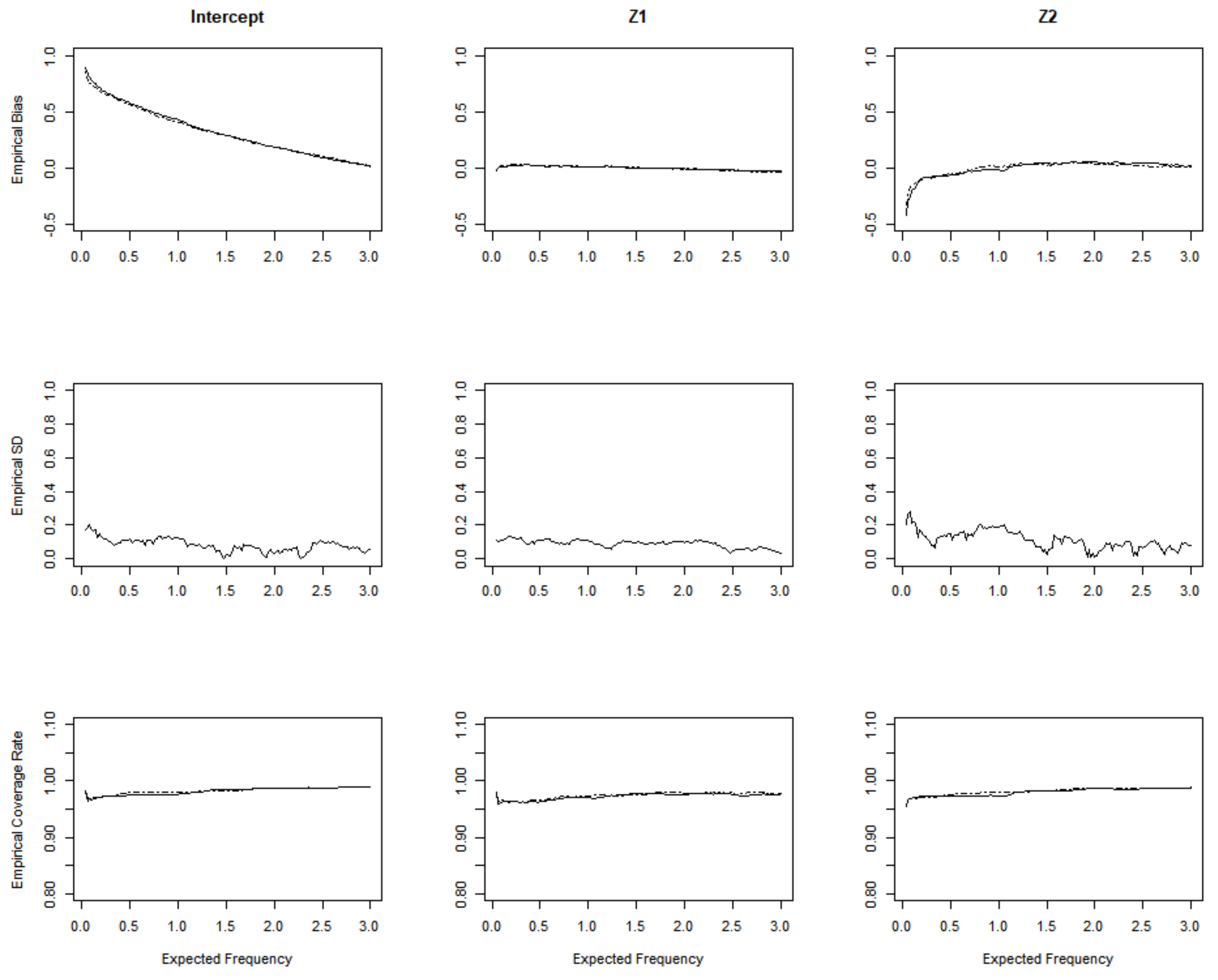
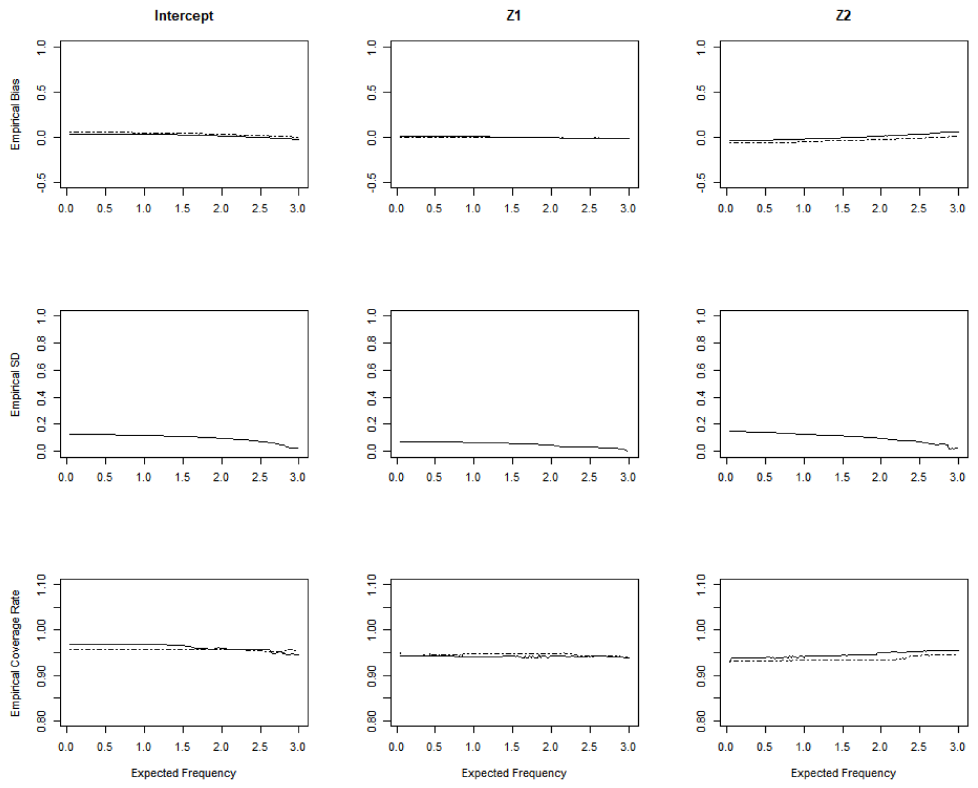
Figure 3 and Figure 4 are the simulation results for the homogeneous Poisson process from the set-up with a Gamma frailty of variance 0 and 0.5. In the first row, we plot the empirical bias of the proposed estimator $\widehat{\beta }\left(u\right)$ (solid lines) and the empirical bias of the Sun’s estimator (dashed lines) [8]. Sun considered the double censored situation while we only consider the right-censored event time to suit a more general situation. In the second row of the plots, we depicted the empirical mean squared error (MSE) versus the expected frequency u. The third row presents the coverage probabilities of 95% confidence intervals obtained from the proposed estimator (solid lines) and Sun’s estimator (dashed lines). We can see that both methods have a slight bias which converges to 0, and the empirical MSE also tends to be stable as u increases. In the homogeneous Poisson process, when the variance of gamma frailty equals 0, the empirical MSE shows less fluctuation compared to the variance that is equal to 0.5.

Figure 5 depicts the same parameters as Figure 3 and Figure 4, while the difference is that the results are from the non-homogeneous Poisson process. We can see that, in the first and second rows of Figure 5, both methods performed quite similarly in terms of the bias and SD. However, from the third row, in terms of the coverage probability, the proposed estimator (solid lines) performed slightly better than the Sun’s estimator (dashed lines), than for the simulation of the non-homogeneous Poisson process.

4. Application to the Bladder Tumor Studies

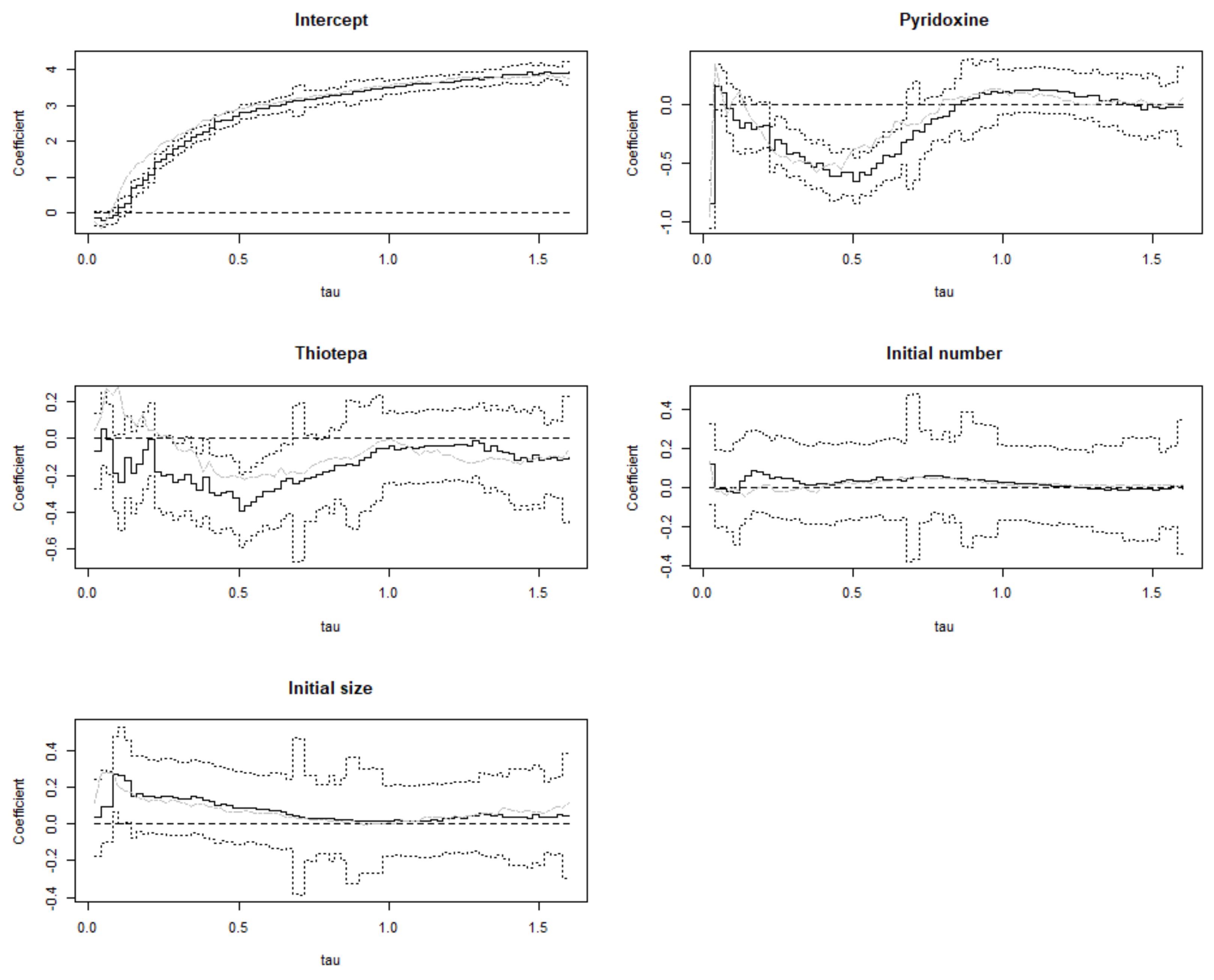
We applied our proposed estimated method to a well-known bladder tumor study [15]. This dataset was conducted to analyze the effect of two treatments, pyridoxine and thiotepa, based on the recurrence of bladder tumors. A total of 118 subjects were recorded, 48 were treated with placebo, 32 were pyridoxine, and 38 with thiotepa. The covariates also contained the initial number of tumors, the size of the largest initial tumor and others. The maximum observed number of recurrences is 9.

We selected four covariates and the intercept: the two treatment methods and the initial tumor size and number. In Figure 6, we displayed our estimation result of the proposed method (solid lines) and Sun’s method (gray line) [8], surrounded by point-wise Wald 95% confidence intervals (dashed lines). The grid-based estimation method estimated the regression coefficients over [0, 1.6]. The intercept coefficient estimates represent the log time to the expected frequency of the bladder tumor recurrence, consisting of patients who had no pyridoxine and thiotepa treatment. The intercept term indicates that as time increases, the bladder tumor recurrence also increases, which is in line with expectations. The negative non-intercept coefficient estimates pyridoxine and thiotepa show that these two treatments can inhibit tumor recurrence. In contrast, the initial tumor size and number of covariates are positive, suggesting a negative effect on tumor recurrence. From Figure 6, we can see that our method and Sun’s method do not have much difference, and the overall trend is the same.

5. Discussion

In this article, we introduced the accelerated recurrence time model for recurrence events, and then considered a new situation when the expected frequency of the accelerated recurrence time model was affected by the time-varying and combined this model with the counting process model. This new counting process model with a non-singleton general function is similar to Cox’s regression model but can be transformed into quantile regression. This method can also estimate more general situations, such as the non-homogeneous Poisson process.

We can generalize our estimation procedure from double-censored to right-censored situations. In the recurrence events setting, the most popular choice of $G(·)$, which may be $G\left(u\right)=u$, as well as $G\left(u\right)=-\ln (1-u)$, we introduce our new estimation method with $G\left(u\right)=ut$. The assumption is that a constant hazard is rarely tenable in practical problems. Therefore, in the parametric estimation process, a more general distribution of the hazard function is the Weibull distribution, which is $g\left(t\right)=\lambda \gamma t^{\gamma -1}$ for $0<t<\infty$, so we have $G\left(u\right)=u{t}^{\gamma }$. When $\gamma =0$, the Weibull distribution function becomes a constant, but resembles the accelerated recurrence time model. When $\gamma =1$, the model became our proposed method. Thus, after combining the parametric and nonparametric methods, we can make the estimation method more diverse and adapt to different types of datasets.

References

- Nelson, W. Hazard plotting for incomplete failure data. J. Qual. Technol. 1969, 1, 27–52. [Google Scholar] [CrossRef]
- Altshuler, B. Theory for the measurement of competing risks in animal experiments. Math. Biosci. 1970, 6, 1–11. [Google Scholar] [CrossRef]
- Lawless, J.F. Regression methods for Poisson process data. J. Am. Stat. Assoc. 1987, 82, 808–815. [Google Scholar] [CrossRef]
- Lin, D.Y.; Wei, L.J.; Yang, I.; Ying, Z. Semiparametric regression for the mean and rate functions of recurrent events. J. R. Stat. Soc. Ser. B (Stat. Methodol.) 2000, 62, 711–730. [Google Scholar] [CrossRef] [Green Version]
- Peng, L.; Huang, Y. Survival analysis with quantile regression models. J. Am. Stat. Assoc. 2008, 103, 637–649. [Google Scholar] [CrossRef]
- Koenker, R.; Bassett, G., Jr. Regression quantiles. Econom. J. Econom. Soc. 1978, 46, 33–50. [Google Scholar] [CrossRef]
- Powell, J.L. Censored regression quantiles. J. Econom. 1986, 32, 143–155. [Google Scholar] [CrossRef]
- Sun, X.; Peng, L.; Huang, Y.; Lai, H.J. Generalizing quantile regression for counting processes with applications to recurrent events. J. Am. Stat. Assoc. 2016, 111, 145–156. [Google Scholar] [CrossRef]
- Wang, H.J.; Wang, L. Locally weighted censored quantile regression. J. Am. Stat. Assoc. 2009, 104, 1117–1128. [Google Scholar] [CrossRef] [Green Version]
- Kim, M.O.; Yang, Y. Semiparametric approach to a random effects quantile regression model. J. Am. Stat. Assoc. 2011, 106, 1405–1417. [Google Scholar] [CrossRef] [PubMed] [Green Version]
- Andersen, P.K.; Gill, R.D. Cox’s regression model for counting processes: A large sample study. Ann. Stat. 1982, 10, 1100–1120. [Google Scholar] [CrossRef]
- Cox, D.R. Regression models and life-tables. J. R. Stat. Soc. Ser. B (Methodol.) 1972, 34, 187–202. [Google Scholar] [CrossRef]
- Huang, Y.; Peng, L. Accelerated recurrence time models. Scand. J. Stat. 2009, 36, 636–648. [Google Scholar] [CrossRef] [PubMed] [Green Version]
- Fygenson, M.; Ritov, Y. Monotone estimating equations for censored data. Ann. Stat. 1994, 22, 732–746. [Google Scholar] [CrossRef]
- Byar, D. The veterans administration study of chemoprophylaxis for recurrent stage i bladder tumours: Comparisons of placebo, pyridoxine and topical thiotepa. In Bladder Tumors and Other Topics in Urological Oncology; Springer: Berlin/Heidelberg, Germany, 1980; pp. 363–370. [Google Scholar]
- Vaart, A.V.D.; Wellner, J.A. Weak convergence and empirical processes with applications to statistics. J. R. Stat. Soc.-Ser. A Stat. Soc. 1997, 160, 596–608. [Google Scholar]
Figure 1.
Estimation results of homogeneous Poisson process.
Figure 2.
Estimation results of non-homogeneous Poisson process.
Figure 3.
Simulation results with sample size n = 100 and the set-up with Gamma frailty of variance 0.
Figure 4.
Simulation results with sample size n = 100 and the set-up with Gamma frailty of variance 0.5.
Figure 5.
Simulation results of non-homogeneous Poisson process with sample size n = 100 and the set-up with Gamma frailty of variance 0.
Figure 6.
Bladder data example: coefficient estimates and 95% pointwise confidence.
Publisher’s Note: MDPI stays neutral with regard to jurisdictional claims in published maps and institutional affiliations. |
© 2022 by the authors. Licensee MDPI, Basel, Switzerland. This article is an open access article distributed under the terms and conditions of the Creative Commons Attribution (CC BY) license (https://creativecommons.org/licenses/by/4.0/).
Share and Cite
MDPI and ACS Style
Wen, X.; Xu, J. Generalized Accelerated Failure Time Models for Recurrent Events. Mathematics 2022, 10, 2662. https://doi.org/10.3390/math10152662
AMA Style
Wen X, Xu J. Generalized Accelerated Failure Time Models for Recurrent Events. Mathematics. 2022; 10(15):2662. https://doi.org/10.3390/math10152662
Chicago/Turabian StyleWen, Xiaoyi, and Jinfeng Xu. 2022. "Generalized Accelerated Failure Time Models for Recurrent Events" Mathematics 10, no. 15: 2662. https://doi.org/10.3390/math10152662
Note that from the first issue of 2016, this journal uses article numbers instead of page numbers. See further details here.