Efficient Estimation and Inference in the Proportional Odds Model for Survival Data

Abstract

In modeling time-to-event data with long-term survivors, the proportional hazards model is widely used for its easy and direct interpretation as well as the flexibility to accommodate the past information and allow time-varying predictors. This becomes most relevant when the mortality of individuals converges with time, and the estimation and inference based upon the proportional odds model can often yield more accurate and reasonable results than the classical Cox’s proportional hazards model. Along with the fast development of the data science technologies, computational challenges for survival data with increasing sample size and diverging parameter dimension exist. Currently, existing methods for analyzing such data are computationally inconvenient. In this paper, we propose efficient computational methods for analyzing survival data in the proportional odds model, where the nonparametric maximum likelihood approach is combined with the minorization-maximization (MM) algorithm and the regularization scheme to yield fast and accurate estimation and inferential procedures. The illustration of the methodology using extensive simulation studies and then the application to the Veterans’ Administration lung cancer data is also given.

1. Introduction

The proportional odds model was initially proposed by McCullagh [1,2] with the purpose of analyzing ordinal data instead of censored survival data. Due to its easy and direct interpretation, it has been widely used in practice. Refs. [3,4] extended the model to fit survival data using the Newton-Raphson method. Many researchers started to use this model in survival analysis also because of its good prediction performance. Ref. [5] considered the rank-based estimation method. Ref. [6] proposed the semi-parametric proportional odds model, which is one important case of the general linear transformation model. In addition, ref. [7] employed the profiled likelihood method and developed the model diagnostic procedures. For interval censored data, refs. [8,9] further introduced the sieve maximum likelihood estimation and obtained the consistency and asymptotic normality for the estimated parameters. Ref. [10] proposed an easy implementation of this proportional odds model based on the conditional logistic regression. Ref. [11] considered the semi-parametric proportional odds model, where the baseline function can be any non-decreasing function. As for the improvement of the parameter estimation efficiency, ref. [12] proposed the minorization-maximization (MM) algorithm for the proportional odds model and this algorithm performswell given high-dimensional data. Ref. [13] adopted the cubic spline for baseline estimation and [14] proposed to capture the spatial heterogeneity using a Bayesian hierarchical model for the analysis of spatially related data. Similarly, ref. [15] also proposed the semiparametric Bayesian proportional odds model, where the baseline is estimated through a monotone increasing spline. The Bayesian model framework was further extended to the application of clustered and multi-event data by [16]. Ref. [17] proposed an extension of the original model in order to fit the data with a multivariate response, random intercept and non-linear effect of covariates. Furthermore, based on the interval censored data and Bayesian estimation method, ref. [18] introduced the cure rate proportional odds models for the corresponding data analysis. Different from the traditional proportional odds model, ref. [19] discussed the quantile-based definition for this model and presented the illustration using real life datasets. Ref. [20] added a log-concave constraint on the baseline distribution and developed the corresponding parameter and density estimation. Besides the MM algorithm, ref. [21] proposed an expectation-maximization (EM) scheme for the parameter estimation with a good computational efficiency for both parameter and baseline estimation. In addition, ref. [22] discussed the efficient estimation of the odds ratio for the proportional odds model with censored time-lagged outcome. [23] has pointed out the high computational complexity and inefficiency for the proportional odds model with right censored data. For example, ref. [7]’s method cannot perform estimation appropriately given the consecutively observed failure time. In addition, ref. [13] pointed out the method proposed by [9] is very complex and computationally unachievable. Moreover, the estimated baseline function from [13]’s method may not preserve the monotone property constructed by the natural cubic spline. Therefore, to tackle these problems, ref. [23] developed the EM algorithm for the proportional odds model with right censored data, where the baseline function is estimated using the spline. The method can be applied to a large dataset, while AIC or BIC criterion is applied to determine the optimal number of knots for the natural cubic spline estimation.

The covariates are important for the regression analysis, where some covariates with a tiny impact to the response might be captured during the estimation procedure. Therefore, when constructing the regression model, it is essential to conduct a variable selection procedure. The most popular way of variable selection is conducted by adding penalty functions to the original objective. The parameters are then estimated by maximizing the new objective function. In the survival analysis, the LASSO [24], SCAD [25], the adaptive LASSO [26] and the elastic SCAD are commonly applied for the proportional hazard models. As for the proportional odds model, only limited studies are conducted based on the penalized regression. Ref. [27] studied the application of LASSO and the adaptive LASSO in the proportional odds model, where the simulation results of the adaptive LASSO demonstrate better performance in both variable selection and parameter estimation.

As for optimizing the likelihood function of the proportional odds model, the Newton-Raphson method and EM algorithm perform well in finding the root without an explicit form. Ref. [28] first developed the MM algorithm to optimize the convex function iteratively. EM algorithm is a special case of the MM algorithm. The MM algorithm can help avoid high-dimensional matrix inversion, separate the parameters, linearize the optimization problem and transform the non-differentiable problem to smooth optimization. In real applications, the MM algorithm has been applied to optimize the objective function from statistical models such as quantile regression [28], Bradley-Terry model [29], zero-inflated and zero-truncated models [30,31], high-dimensional covariates selection problem [32], mixed Gaussian model [33] and finite mixture models. In addition, the MM algorithm has been also applied to survival analysis. Ref. [34] has developed a MM algorithm to solve the optimization problem based on the shared gamma frailty model. The estimation results perform well in their simulation and real data analysis.

In the following article, we first review the MM algorithm in Section 2. Then, we apply the usage of the MM algorithm in the proportional odds model in Section 3. In Section 4, we further conduct a variable selection procedure based on the proportional odds model using the MM algorithm. Simulation studies and real data analysis are conducted in Section 5 and Section 6. Finally, we conclude the performance of our proposed methods and discuss the future work in Section 7.

2. MM Algorithm

2.1. Basic Principle

The MM algorithm performs optimization by constructing a simple surrogate function for the original objective function. Then, instead of optimizing the original objective function, we optimize the surrogate function with simplified expression. The process of the MM algorithm involves two steps; the first M step is the minorization step, which constructs a proper minorization function under the following conditions (1) and (2) by some commonly used inequations. The second M step is the maximization step, where a minorization function is maximized via the Newton-Raphson method or a quasi-Newton method, since the constructed minorization function is usually parameter-separable.

Let $\ell \left(\mathit{\theta }\mid Y_{\mathrm{obs}}\right)$ is the log-likelihood of observed data $Y_{obs}$, $\widehat{\theta }$ is the parameter estimation through the maximization of log-likelihood. Assume ${\mathit{\theta }}^{\left(t\right)}$ is the t-th iteration of $\widehat{\mathit{\theta }}$, $Q\left(\mathit{\theta }\mid {\mathit{\theta }}^{\left(t\right)}\right)$ is the surrogate function determined by ${\mathit{\theta }}^{\left(t\right)}$. If ${\mathit{\theta }}^{\left(t\right)}$ satisfy,

$$\begin{array}{cc}\hfill Q\left(\mathit{\theta }\mid {\mathit{\theta }}^{\left(t\right)}\right)& ⩽\ell \left(\mathit{\theta }\mid Y_{\mathrm{obs}}\right)\forall \mathit{\theta },{\mathit{\theta }}^{\left(t\right)}\in \mathsf{\Theta },\mathrm{and}\hfill \end{array}$$

(1)

$$\begin{array}{cc}\hfill Q\left({\mathit{\theta }}^{\left(t\right)}\mid {\mathit{\theta }}^{\left(t\right)}\right)& =\ell \left({\mathit{\theta }}^{\left(t\right)}\mid Y_{\mathrm{obs}}\right).\hfill \end{array}$$

(2)

Then, we call $Q\left(\mathit{\theta }\mid {\mathit{\theta }}^{\left(t\right)}\right)$ to be the minorization function of $\ell \left(\mathit{\theta }\mid Y_{\mathrm{obs}}\right)$. The maximizing of $Q\left(\mathit{\theta }\mid {\mathit{\theta }}^{\left(t\right)}\right)$ can substitute the maximization of the original objective. If $Q\left(\mathit{\theta }\mid {\mathit{\theta }}^{\left(t\right)}\right)$ obtains the optimal at ${\mathit{\theta }}^{(t+1)}$,

$${\mathit{\theta }}^{(t+1)}=\arg \underset{\mathit{\theta }\in \mathsf{\Theta }}{\max }Q\left(\mathit{\theta }\mid {\mathit{\theta }}^{\left(t\right)}\right).$$

From (1) and (2), we have

$$\ell \left({\mathit{\theta }}^{(t+1)}\mid Y_{\mathrm{obs}}\right)⩾Q\left({\mathit{\theta }}^{(t+1)}\mid {\mathit{\theta }}^{\left(t\right)}\right)⩾Q\left({\mathit{\theta }}^{\left(t\right)}\mid {\mathit{\theta }}^{\left(t\right)}\right)=\ell \left({\mathit{\theta }}^{\left(t\right)}\mid Y_{\mathrm{obs}}\right).$$

The MM algorithm is a stable optimization procedure and has a convergence property due to the increase in the objective in every iteration. EM algorithm is a special case of MM algorithm and its first M step (also called E step) is to calculate the expectation of the complete-data log-likelihood function.

2.2. Commonly Used Inequalities

The key step of the MM algorithm is to find the appropriate surrogate function for the objective with less computational cost. In real applications, in order to construct the surrogate function, we suggest the following ways based on the commonly used algebraic inequalities.

The first method is Jensen’s inequality. Assume that X is a random variable, and $\phi$ is a concave function, then

$$\phi \left(\mathrm{E}\right[X\left]\right)\ge \mathrm{E}\left[\phi \right(X\left)\right].$$

In contrast, if $\phi$ is convex, then,

$$\phi \left(\mathrm{E}\right[X\left]\right)\le \mathrm{E}\left[\phi \right(X\left)\right].$$

In real applications, we always use the continuous and discrete version of Jensen’s Inequality. The continuous version is

$$\phi \left({\int }_{\mathsf{\Omega }}f\left(x\right)·g\left(x\right)\mathrm{d}x\right)\ge {\int }_{\mathsf{\Omega }}\phi \left(f\left(x\right)\right)·g\left(x\right)\mathrm{d}x,$$

where $\mathsf{\Omega }$ is the subset of the real line $\mathbb{R}$. $f(·)$ is defined real function on $\mathsf{\Omega }$, $g(·)$ is the density function on $\mathsf{\Omega }$. Discrete version,

$$\phi \left({\displaystyle \sum _{i=1}^n}{a}_i{x}_i\right)\ge {\displaystyle \sum _{i=1}^n}{a}_i\phi \left(x_i\right),$$

where $\phi (·)$ is a concave function, $a_i\ge 0$ and ${\displaystyle \sum _{i=1}^n}{a}_i=1$.

The second method is the inequality of arithmetic and geometric means,

$$-{\displaystyle \prod _{i=1}^n}{x}_i^{a_i}\ge -{\displaystyle \sum _{i=1}^n}\frac{a_i}{{\parallel \mathit{a}\parallel }_1}{x}_i^{{\parallel \mathit{a}\parallel }_1}.$$

where $x_i$ and $a_i$ are nonnegative. The left-hand side of the inequality is a product of $x_i^{a_i}$ and the other side of this inequality is the sum of $x_i^{{\parallel \mathit{a}\parallel }_1}$ for $i=1,\dots ,n$. The structure of this inequality says that it can be used to minorize product terms into the summation of other terms.

The third method is the supporting hyperplane inequality,

$$-\log \left(x\right)\ge -\log \left(x_0\right)-\frac{x-x_0}{x_0}.$$

3. Proportional Odds Model

Let T denotes the failure time, X is the covariate of $p\times 1$ dimension, $\mathit{\beta }$ is the corresponding coefficient. Suppose that given X, T follow the proportional odds model

$$\mathrm{logit}\left\{F(t\mid X)\right\}=\log {\mathsf{\Lambda }}_0\left(t\right)+X^{\top }\mathit{\beta },$$

where $F(t\mid X)$ denotes the cumulative distribution function of T given X, ${\mathsf{\Lambda }}_0\left(t\right)$ denotes a cumulative baseline function, and $\mathrm{logit}\left(x\right)=\log \frac{x}{1-x}$.

Based on the assumption above, we can easily obtain the survival and density function of the proportional odds model

$$S(t\mid X)=\frac{1}{1+{\mathsf{\Lambda }}_0\left(t\right)\exp \left(X^{\top }\mathit{\beta }\right)}$$

and

$$f(t\mid X)=\frac{{\lambda }_0\left(t\right)\exp \left(X^{\top }\mathit{\beta }\right)}{{\left[1+{\mathsf{\Lambda }}_0\left(t\right)\exp \left(X^{\top }\mathit{\beta }\right)\right]}^2},$$

respectively, with the hazard rate

$$\lambda (t\mid X)=\frac{{\lambda }_0\left(t\right)\exp \left(X^{\top }\mathit{\beta }\right)}{1+{\mathsf{\Lambda }}_0\left(t\right)\exp \left(X^{\top }\mathit{\beta }\right)},$$

where ${\lambda }_0\left(t\right)=\mathrm{d}{\mathsf{\Lambda }}_0(t)/\mathrm{d}t$.

Here, we consider the failure time T with a right censoring structure, and a failure time study that consists of n independent individuals. Let $T_i$, $C_i$ and $X_i$ denote the failure time, the censoring time and the covariate of the $i^{th}$ individual, respectively. Moreover, we assume the $T_i$ and $C_i$ are independent. In addition, let $t_i=\min \left(T_i,C_i\right)$ denote the observation time of event, and ${\delta }_i=I\left(T_i\le C_i\right)$ is the censoring indicator based on the observed data $\left\{t_i,{\delta }_i,X_i\right\}$, $i=1,\dots ,n$. Then, the likelihood function is

$$L_{obs}={\displaystyle \prod _{i=1}^n}{\left\{\frac{{\lambda }_0\left(t_i\right)\exp \left(X_i^{\top }\mathit{\beta }\right)}{1+{\mathsf{\Lambda }}_0\left(t_i\right)\exp \left(X_i^{\top }\mathit{\beta }\right)}\right\}}^{{\delta }_i}\frac{1}{1+{\mathsf{\Lambda }}_0\left(t_i\right)\exp \left(X_i^{\top }\mathit{\beta }\right)}.$$

with the corresponding log-likelihood function

$${\ell }_{obs}={\displaystyle \sum _{i=1}^n}\left\{{\delta }_i\log {\lambda }_0\left(t_i\right)+{\delta }_i{X}_i^{\top }\mathit{\beta }-\left({\delta }_i+1\right)\log \left[1+{\mathsf{\Lambda }}_0\left(t_i\right)\exp \left(X_i^{\top }\mathit{\beta }\right)\right]\right\}.$$

(3)

In Equation (3), using the supporting hyperplane inequality,

$$-\log \left(x\right)\ge -\log \left(x_0\right)-\frac{x-x_0}{x_0}.$$

we have

$$\begin{array}{cc}\hfill -\left({\delta }_i+1\right)\log \left[1+{\mathsf{\Lambda }}_0\left(t_i\right)\exp \left(X_i^{\top }\mathit{\beta }\right)\right]\ge & -\left({\delta }_i+1\right)\log (A_i^{\left(k\right)})\hfill \\ & -\left({\delta }_i+1\right)\frac{1+{\mathsf{\Lambda }}_0\left(t_i\right)\exp \left(X_i^{\top }\mathit{\beta }\right)-A_i^{\left(k\right)}}{A_i^{\left(k\right)}},\hfill \end{array}$$

where $A_i^{\left(k\right)}=1+{\mathsf{\Lambda }}_0^{\left(k\right)}\left(t_i\right)\exp \left(X_i^{\top }{\mathit{\beta }}^{\left(k\right)}\right)$. Then, we can obtain the surrogate function of ${\ell }_{obs}$, as follows

$$Q_{11}({\mathsf{\Lambda }}_0,\mathit{\beta }\mid {\mathsf{\Lambda }}_0^{\left(k\right)},{\mathit{\beta }}^{\left(k\right)})={\displaystyle \sum _{i=1}^n}\left\{{\delta }_i\log {\lambda }_0\left(t_i\right)+{\delta }_i{X}_i^{\top }\mathit{\beta }-\frac{\left({\delta }_i+1\right){\mathsf{\Lambda }}_0\left(t_i\right)\exp \left(X_i^{\top }\mathit{\beta }\right)}{A_i^{\left(k\right)}}\right\}.$$

After the minimization step, we then apply two methods to estimate the surrogate function derived above.

3.1. Profile MM Method

Given the value of $\mathit{\beta }$, we can obtain the estimate of ${\mathsf{\Lambda }}_0$

$$d{\widehat{\mathsf{\Lambda }}}_0\left(t_i\right)=\frac{{\delta }_i}{{\displaystyle \sum _{j=1}^n}I\left(t_j⩾t_i\right)\left({\delta }_j+1\right)\exp \left(X_j^{\top }\mathit{\beta }\right)/A_j^{\left(k\right)}}.$$

(4)

Substitute (4) into $Q_{11}\left({\mathsf{\Lambda }}_0,\mathit{\beta }\mid {\mathsf{\Lambda }}_0^{\left(k\right)},{\mathit{\beta }}^{\left(k\right)}\right)$, we have

$$Q_{12}\left(\mathit{\beta }\mid {\mathsf{\Lambda }}_0^{\left(k\right)},{\mathit{\beta }}^{\left(k\right)}\right)={\displaystyle \sum _{i=1}^n}{\delta }_i{X}_i^{\top }\mathit{\beta }-{\displaystyle \sum _{i=1}^n}\left\{{\delta }_i\log {\displaystyle \sum _{j=1}^n}I\left(t_j⩾t_i\right)\left({\delta }_j+1\right)\exp \left(X_j^{\top }\mathit{\beta }\right)/A_j^{\left(k\right)}\right\}+c_1,$$

where $c_1$ is a constant. Using the supporting hyperplane inequality again to minimize $Q_{12}\left(\mathit{\beta }\mid {\mathsf{\Lambda }}_0^{\left(k\right)},{\mathit{\beta }}^{\left(\mathit{k}\right)}\right)$, we have

$$Q_{13}\left(\mathit{\beta }\mid {\mathsf{\Lambda }}_0^{\left(k\right)},{\mathit{\beta }}^{\left(k\right)}\right)={\displaystyle \sum _{i=1}^n}{\delta }_i{X}_i^{\top }\mathit{\beta }-{\displaystyle \sum _{i=1}^n}\frac{{\delta }_i{\displaystyle \sum _{j=1}^n}I\left(t_j⩾t_i\right)\left({\delta }_j+1\right)\exp \left(X_j^{\top }\mathit{\beta }\right)/A_j^{\left(k\right)}}{B_i^{\left(k\right)}}+c_2,$$

(5)

where $c_2$ is a constant and $B_i^{\left(k\right)}={\displaystyle \sum _{j=1}^n}I\left(t_j⩾t_i\right)\left({\delta }_j+1\right)\exp \left(X_j^{\top }\mathit{\beta }\right)/A_j^{\left(k\right)}$.

Taking first and second derivatives for $Q_{13}\left(\mathit{\beta }\mid {\mathsf{\Lambda }}_0^{\left(k\right)},{\mathit{\beta }}^{\left(k\right)}\right)$ to $\mathit{\beta }$, then

$$\begin{array}{cc}\hfill Q_{13}^{\prime }\left(\mathit{\beta }\mid {\mathsf{\Lambda }}_0^{\left(k\right)},{\mathit{\beta }}^{\left(k\right)}\right)& ={\displaystyle \sum _{i=1}^n}{\delta }_i{X}_i^{\top }-{\displaystyle \sum _{i=1}^n}\frac{{\delta }_i{\displaystyle \sum _{j=1}^n}I\left(t_j⩾t_i\right)\left({\delta }_j+1\right)\exp \left(X_j^{\top }\mathit{\beta }\right)X_j^{\top }/A_j^{\left(k\right)}}{B_i^{\left(k\right)}},\hfill \\ \hfill Q_{13}^{″}\left(\mathit{\beta }\mid {\mathsf{\Lambda }}_0^{\left(k\right)},{\mathit{\beta }}^{\left(k\right)}\right)& =-{\displaystyle \sum _{i=1}^n}\frac{{\delta }_i{\displaystyle \sum _{j=1}^n}I\left(t_j⩾t_i\right)\left({\delta }_j+1\right)\exp \left(X_j^{\top }\mathit{\beta }\right)X_j^{\top }{X}_j/A_j^{\left(k\right)}}{B_i^{\left(k\right)}}.\hfill \end{array}$$

The estimation function for $\mathit{\beta }$ is

$${\mathit{\beta }}^{(k+1)}={\mathit{\beta }}^{\left(k\right)}-Q_{13}^{″}{\left({\mathit{\beta }}^{\left(k\right)}\mid {\mathsf{\Lambda }}_0^{\left(k\right)},{\mathit{\beta }}^{\left(k\right)}\right)}^{-1}{Q}_{13}^{\prime }\left({\mathit{\beta }}^{\left(k\right)}\mid {\mathsf{\Lambda }}_0^{\left(k\right)},{\mathit{\beta }}^{\left(k\right)}\right).$$

The algorithm is given below,

• Let the initial value for $(\mathit{\beta },{\mathsf{\Lambda }}_0)$ be $({\mathit{\beta }}^{\left(0\right)},{\mathsf{\Lambda }}_0^{\left(0\right)})$.
• Update the estimate of $\mathit{\beta }$ by Equation (5).
• Using the updated value of $\mathit{\beta }$, calculate the estimate of ${\mathsf{\Lambda }}_0$ by Equation (4).
• Iterate step 2 and 3 until it converges.

3.2. Non-Profile MM Method

Use the inequality of arithmetic and geometric means

$$-{\displaystyle \prod _{i=1}^n}{x}_i^{a_i}\ge -{\displaystyle \sum _{i=1}^n}\frac{a_i}{{\parallel \mathit{a}\parallel }_1}{x}_i^{{\parallel \mathit{a}\parallel }_1}$$

to minimize $Q_{11}({\mathsf{\Lambda }}_0,\mathit{\beta }\mid {\mathsf{\Lambda }}_0^{\left(k\right)},{\mathit{\beta }}^{\left(k\right)})$, let $x_1={\mathsf{\Lambda }}_0\left(t_i\right)/{\mathsf{\Lambda }}_0^{\left(k\right)}\left(t_i\right)$ and $x_2=\exp \left(X_i^{\top }\mathit{\beta }\right)/\exp \left(X_i^{\top }{\mathit{\beta }}^{\left(k\right)}\right)$, we have

$$-\frac{{\mathsf{\Lambda }}_0\left(t_i\right)\exp \left(X_i^{\top }\mathit{\beta }\right)}{{\mathsf{\Lambda }}_0^{\left(k\right)}\left(t_i\right)\exp \left(X_i^{\top }{\mathit{\beta }}^{\left(k\right)}\right)}\ge -\frac{{\mathsf{\Lambda }}_0^2\left(t_i\right)}{2{\mathsf{\Lambda }}_0^{2\left(k\right)}\left(t_i\right)}-\frac{\exp \left(2X_i^{\top }{\mathit{\beta }}^{\left(k\right)}\right)}{2\exp \left(2X_i^{\top }{\mathit{\beta }}^{\left(k\right)}\right)}.$$

By computation, we obtain

$$-{\mathsf{\Lambda }}_0\left(t_i\right)\exp \left(X_i^{\top }\mathit{\beta }\right)\ge -\frac{\exp \left(X_i^{\top }{\mathit{\beta }}^{\left(k\right)}\right)}{2{\mathsf{\Lambda }}_0^{\left(k\right)}\left(t_i\right)}{\mathsf{\Lambda }}_0^2\left(t_i\right)-\frac{{\mathsf{\Lambda }}_0^{\left(k\right)}\left(t_i\right)}{2\exp \left(X_i^{\top }{\mathit{\beta }}^{\left(k\right)}\right)}\exp \left(2X_i^{\top }\mathit{\beta }\right).$$

Therefore, the surrogate function is

$$\begin{array}{c}\hfill Q_{14}({\mathsf{\Lambda }}_0,\mathit{\beta }\mid {\mathsf{\Lambda }}_0^{\left(k\right)},{\mathit{\beta }}^{\left(k\right)})=Q_{14}({\mathsf{\Lambda }}_0\mid {\mathsf{\Lambda }}_0^{\left(k\right)},{\mathit{\beta }}^{\left(k\right)})+Q_{14}(\mathit{\beta }\mid {\mathsf{\Lambda }}_0^{\left(k\right)},{\mathit{\beta }}^{\left(k\right)}),\end{array}$$

where

$$\begin{array}{cc}\hfill Q_{14}({\mathsf{\Lambda }}_0\mid {\mathsf{\Lambda }}_0^{\left(k\right)},{\mathit{\beta }}^{\left(k\right)})=& {\displaystyle \sum _{i=1}^n}{\delta }_i\log {\lambda }_0\left(t_i\right)-{\displaystyle \sum _{i=1}^n}\frac{({\delta }_i+1)\exp \left(X_i^{\top }{\mathit{\beta }}^{\left(k\right)}\right)}{2A_i^{\left(k\right)}{\mathsf{\Lambda }}_0^{\left(k\right)}}{\mathsf{\Lambda }}_0^2,\hfill \end{array}$$

$$\begin{array}{cc}\hfill Q_{14}(\mathit{\beta }\mid {\mathsf{\Lambda }}_0^{\left(k\right)},{\mathit{\beta }}^{\left(k\right)})=& {\displaystyle \sum _{i=1}^n}{\delta }_i{X}_i^{\top }\mathit{\beta }-{\displaystyle \sum _{i=1}^n}\frac{({\delta }_i+1){\mathsf{\Lambda }}_0^{\left(k\right)}}{2A_i^{\left(k\right)}\exp \left(X_i^{\top }{\mathit{\beta }}^{\left(k\right)}\right)}\exp \left(2X_i^{\top }\mathit{\beta }\right).\hfill \end{array}$$

(6)

Let $\frac{\partial Q_{14}({\mathsf{\Lambda }}_0,\mathit{\beta }\mid {\mathsf{\Lambda }}_0^{\left(k\right)},{\mathit{\beta }}^{\left(k\right)})}{\partial {\mathsf{\Lambda }}_0}=0$, the estimation equation of ${\mathsf{\Lambda }}_0$ is

$$d{\widehat{\mathsf{\Lambda }}}_0\left(t_i\right)=\frac{{\delta }_i}{{\displaystyle \sum _{j=1}^n}I\left(t_j⩾t_i\right)\left({\delta }_j+1\right)\exp \left(X_j^{\top }\mathit{\beta }\right)/A_j^{\left(k\right)}}.$$

(7)

The first and second derivatives of $\mathit{\beta }$ are

$$\begin{array}{cc}\hfill Q_{14}^{\prime }(\mathit{\beta }\mid {\mathsf{\Lambda }}_0^{\left(k\right)},{\mathit{\beta }}^{\left(k\right)})& ={\displaystyle \sum _{i=1}^n}{\delta }_i{X}_i^{\top }-{\displaystyle \sum _{i=1}^n}\frac{({\delta }_i+1){\mathsf{\Lambda }}_0^{\left(k\right)}}{A_i^{\left(k\right)}\exp \left(X_i^{\top }{\mathit{\beta }}^{\left(k\right)}\right)}\exp \left(2X_i^{\top }\mathit{\beta }\right)X_i^{\top },\hfill \\ \hfill Q_{14}^{″}(\mathit{\beta }\mid {\mathsf{\Lambda }}_0^{\left(k\right)},{\mathit{\beta }}^{\left(k\right)})& =-{\displaystyle \sum _{i=1}^n}\frac{2({\delta }_i+1){\mathsf{\Lambda }}_0^{\left(k\right)}}{A_i^{\left(k\right)}\exp \left(X_i^{\top }{\mathit{\beta }}^{\left(k\right)}\right)}\exp \left(2X_i^{\top }\mathit{\beta }\right)X_i^{\top }{X}_i.\hfill \end{array}$$

Thus, we have the estimation function of $\mathit{\beta }$ which is

$${\mathit{\beta }}^{(k+1)}={\mathit{\beta }}^{\left(k\right)}-Q_{14}^{″}{({\mathit{\beta }}^{\left(k\right)}\mid {\mathsf{\Lambda }}_0^{\left(k\right)},{\mathit{\beta }}^{\left(k\right)})}^{-1}{Q}_{14}^{\prime }({\mathit{\beta }}^{\left(k\right)}\mid {\mathsf{\Lambda }}_0^{\left(k\right)},{\mathit{\beta }}^{\left(k\right)}).$$

The algorithm is as follows,

• Let the initial value of $(\mathit{\beta },{\mathsf{\Lambda }}_0)$ to be $({\mathit{\beta }}^{\left(0\right)},{\mathsf{\Lambda }}_0^{\left(0\right)})$.
• Update $\mathit{\beta }$ using Equation (6).
• Use the updated value of $\mathit{\beta }$, calculate the estimate of ${\mathsf{\Lambda }}_0$ using Equation (7).
• Iterate step 2 and 3 until convergence.

To sum up, both profile MM and non-profile MM methods have decomposed the objective function into two separate parts. That is, the non-parametric component ${\mathsf{\Lambda }}_0$ is separated from the regression vector $\mathit{\beta }$, which makes the next maximization step more simple than directly optimizing the objective log-likelihood function. It is worth noting that the parameter-separable feature is one of the advantages of the MM algorithm, which can easily incorporate the quasi-Newton acceleration and other simple off-the-shelf accelerators for boosting computational effectiveness.

4. Variable Selection in the Proportional Odds Model

4.1. Parameter Separated Estimation Method

Notice that the estimate of $\mathit{\beta }$ relies on the Newton-Raphson algorithm, which is sensitive to the initial value, and may lead to computational inefficiency due to the inappropriate choice of initial value. Particularly, the higher the dimension of $\mathit{\beta }$, the higher order the matrix of Henssian from the Newton-Raphson method with a high computational cost in doing matrix inverse. Under this circumstance, the proposed MM method can avoid such a matrix inversion problem with much lower computational cost. In the following section, we describe in detail on the parameter-separated estimation method following the previous two methods of Section 3.

First, let

$$X_i^{\top }\mathit{\beta }={\displaystyle \sum _{q=1}^p}{\omega }_{iq}\left[{\omega }_{iq}^{-1}{x}_{iq}({\mathit{\beta }}_q-{\mathit{\beta }}_q^{\left(k\right)})+X_i^{\top }{\mathit{\beta }}^{\left(k\right)}\right],$$

(8)

when $x_{iq}=0$, we let $1/{\omega }_{iq}=0$. Then, using the discrete form of Jensen’s inequality,

$$\phi \left({\displaystyle \sum _{i=1}^n}{a}_i{x}_i\right)\ge {\displaystyle \sum _{i=1}^n}{a}_i\phi \left(x_i\right),$$

(9)

where, $\phi (·)$ is a concave function, $a_i\ge 0$ and ${\displaystyle \sum _{i=1}^n}{a}_i=1$.

Let $\phi (·)=-\exp (·)$ in Equation (9) and use the expression form of Equation (8), we can minimize Equation (5) by

$$Q_{15}(\mathit{\beta }\mid {\mathsf{\Lambda }}_0^{\left(k\right)},{\mathit{\beta }}^{\left(k\right)})={\displaystyle \sum _{q=1}^p}{Q}_{15q}({\mathit{\beta }}_q\mid {\mathsf{\Lambda }}_0^{\left(k\right)},{\mathit{\beta }}^{\left(k\right)}),$$

(10)

where

$$\begin{array}{cc}& Q_{15q}({\mathit{\beta }}_q\mid {\mathsf{\Lambda }}_0^{\left(k\right)},{\mathit{\beta }}^{\left(k\right)})\hfill \\ & ={\displaystyle \sum _{i=1}^n}\left\{{\delta }_i{x}_{iq}{\mathit{\beta }}_q-\frac{{\delta }_i{\displaystyle \sum _{j=1}^n}I\left(t_j⩾t_i\right)\left({\delta }_j+1\right){\omega }_{jq}\exp ({\omega }_{jq}^{-1}{x}_{jq}({\mathit{\beta }}_q-{\mathit{\beta }}_q^{\left(k\right)})+X_i^{\top }{\mathit{\beta }}^{\left(k\right)})/A_j^{\left(k\right)}}{B_i^{\left(k\right)}}\right\}.\hfill \end{array}$$

Similarly, let $\phi (·)=-\exp (·)$ in Equation (9) and use the expression form of Equation (8), we can also minimize Equation (6) by

$$Q_{16}(\mathit{\beta }\mid {\mathsf{\Lambda }}_0^{\left(k\right)},{\mathit{\beta }}^{\left(k\right)})={\displaystyle \sum _{q=1}^p}{Q}_{16q}({\mathit{\beta }}_q\mid {\mathsf{\Lambda }}_0^{\left(k\right)},{\mathit{\beta }}^{\left(k\right)}),$$

(11)

where

$$\begin{array}{cc}& Q_{16q}({\mathit{\beta }}_q\mid {\mathsf{\Lambda }}_0^{\left(k\right)},{\mathit{\beta }}^{\left(k\right)})\hfill \\ & ={\displaystyle \sum _{i=1}^n}\left\{{\delta }_i{x}_{iq}{\mathit{\beta }}_q-\frac{({\delta }_i+1){\mathsf{\Lambda }}_0^{\left(k\right)}}{2A_i^{\left(k\right)}\exp \left(X_i^{\top }{\mathit{\beta }}^{\left(k\right)}\right)}{\omega }_{iq}\exp (2{\omega }_{iq}^{-1}{x}_{iq}({\mathit{\beta }}_q-{\mathit{\beta }}_q^{\left(k\right)})+2X_i^{\top }{\mathit{\beta }}^{\left(k\right)})\right\}.\hfill \end{array}$$

From Equations (10) and (11), it can be observed that the two resulting MM methods only involves $p+1$ separate univariate optimizations in its maximization step and matrix inversion is not needed. Thus, the proposed methods can highly reduce the computational cost.

4.2. The Variable Selection Based on SCAD and MCP Penalties

The variable selection is an important field in high-dimensional data analysis. Using variable selection methods to select significant explanatory variables and remove the insignificant ones can improve the prediction accuracy of the statistical model. In this article, we applied the SCAD and MCP penalties with oracle properties to conduct variable selection in the proportional odds model. The penalized log-likelihood function becomes the new objective to be minimized, which can be written as,

$${\ell }_{pen}\left(\mathit{\beta }\right)={\ell }_{obs}\left(\mathit{\beta }\right)-n{\displaystyle \sum _{q=1}^p}\rho (\left|{\mathit{\beta }}_q\right|\mid ϵ,\gamma ),$$

where $\rho (·\mid ϵ,\gamma )$ is the penalized term. Where the SCAD proposed by [35] is

$$\rho (t\mid ϵ)=ϵ{\int }_0^t\min \left\{1,\frac{{(\gamma -x/ϵ)}_{+}}{\gamma -1}\right\}\mathrm{d}x,t\ge 0,ϵ\ge 0,\gamma \ge 2,$$

$\gamma$ is suggested to take value 3.7 and the MCP proposed by [36] is

$$\rho (t\mid ϵ)=ϵ{\int }_0^t(1-\frac{x}{ϵ\gamma })\mathrm{d}x,t\ge 0,ϵ\ge 0,\gamma >1,$$

where $\gamma$ here takes 3.

In order to handle the singularity around the origin of $\rho (\left|{\mathit{\beta }}_q\right|\mid ϵ,\gamma )$, [35] suggested to use the quadratic local approximation of the penalized term, which can be written as

$$-\rho \left(\left|{\mathit{\beta }}_q\right|\mid ϵ,\gamma \right)\ge -\rho \left(\left|{\mathit{\beta }}_q^{\left(k\right)}\right|\mid ϵ,\gamma \right)-\frac{{\rho }^{\prime }\left(\left|{\mathit{\beta }}_q^{\left(k\right)}\right|\mid ϵ,\gamma \right)}{2\left|{\mathit{\beta }}_q^{\left(k\right)}\right|}\left({\mathit{\beta }}_q^2-{\mathit{\beta }}_q^{\left(k\right)2}\right).$$

Thus, the penalized surrogate function can be written as

$$Q_{pen}\left(\mathit{\beta }\right)={\ell }_{obs}\left(\mathit{\beta }\right)-n{\displaystyle \sum _{q=1}^p}\frac{{\rho }^{\prime }\left(\left|{\mathit{\beta }}_q^{\left(k\right)}\right|\mid ϵ,\gamma \right)}{2\left|{\mathit{\beta }}_q^{\left(k\right)}\right|}{\mathit{\beta }}_q^2.$$

where ${\ell }_{obs}\left(\mathit{\beta }\right)$ can be minorized by Equation (10) or Equation (11).

In order to obtain a good variable selection result, we applied the BIC criterion to select the tuning parameter $ϵ$. The likelihood function with BIC criterion suggested by [37] is

$$BIC=-2\ell ({\widehat{\mathsf{\Lambda }}}_0,\widehat{\mathit{\beta }})+q\log \left(n\right),$$

where n is the sample size and q denotes the dimension of $\widehat{\mathit{\beta }}$, which is the number of selected non-zero parameters. For the exact process of tuning parameters’ selection, we first find the the proper range of $\lambda$ values by searching from $(0,+\infty )$ using this BIC criteria with an initial sequence $s_1,s_2,\dots ,s_{k_1}$. The solution path can be plotted using this sequence and $s_i$ is selected where the minimum BIC is obtained. Then, some grid points are constructed in a range $(s_{i-1},s_{i+1})$ for a more accurate search where the optimal $\lambda$ is selected from this sequence with the minimum BIC score.

5. Simulation Study

According to the estimation equation derived in previous sections, we simulate the data to analyze the estimation result at a finite sample size.

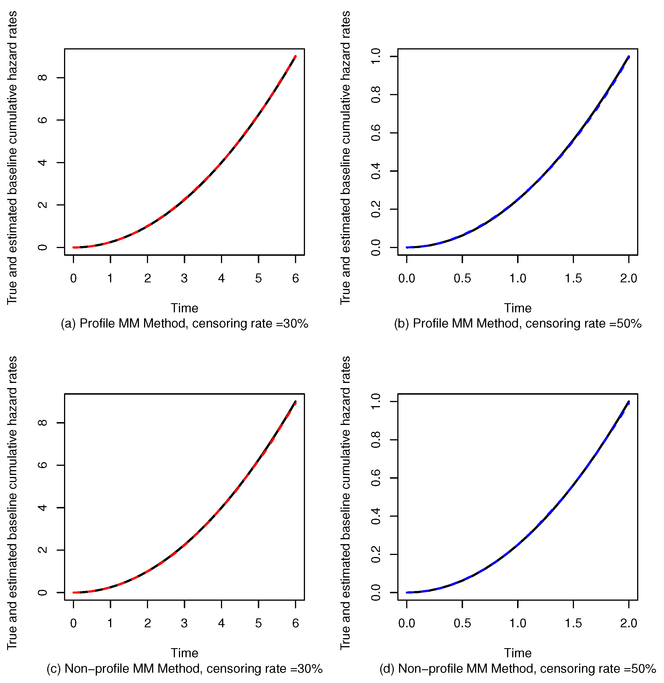
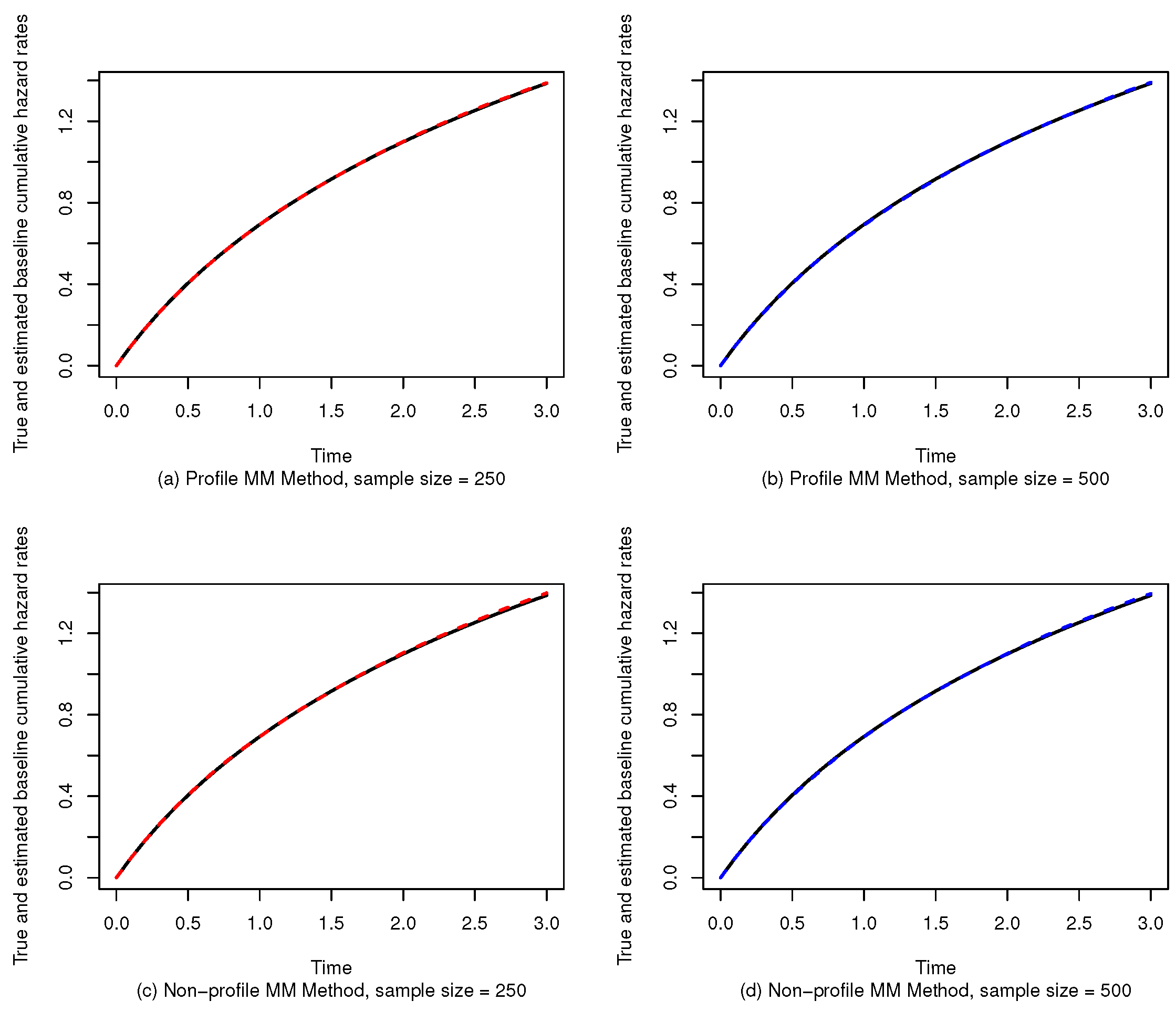
5.1. Parameter Estimation of the Proportional Odds Model

Case 1: The data is simulated to verify the method given from Section 3. Let ${(X_1,X_2,X_3)}^{\top }$ be the covariates, which follow the standard normal distribution and the true parameter $\mathit{\beta }$ is set to be ${(2,1,-3)}^{\top }$, ${\mathsf{\Lambda }}_0\left(t\right)={(t/2)}^2$. The censoring times are generated from the uniform distribution $\mathrm{U}(0,b)$ to yield two censoring proportions of about $30\%$ or $50\%$ separately. We take sample size to be 250 and 500, the corresponding censoring rate are 30% and 50%. The simulation is conducted 500 times repeatedly. The BIAS, MSE (mean square error), SD (standard deviation) and median number of iterations (K) are reported in the following

Table 1. The estimation result of Case 1 with 30% censoring rate.

n	Parameter	Profile MM				Non-Profile MM
		BIAS	MSE	SD	K	BIAS	MSE	SD	K
250	${\beta }_1$	−0.0066	0.0316	0.1777		0.0024	0.0324	0.1801
	${\beta }_2$	−0.0077	0.0204	0.1426		0.0092	0.0182	0.1348
	${\beta }_3$	−0.0001	0.0513	0.2267	104	−0.0139	0.0486	0.2203	298
	${\mathsf{\Lambda }}_0\left(0.5\right)$	0.0085	0.0003	0.0172		0.0002	0.0003	0.0166
	${\mathsf{\Lambda }}_0\left(1\right)$	0.0052	0.0035	0.0593		0.0004	0.0028	0.0528
500	${\beta }_1$	−0.0068	0.0143	0.1195		−0.0085	0.0151	0.1226
	${\beta }_2$	0.0007	0.0089	0.0943		0.0016	0.0101	0.1008
	${\beta }_3$	−0.0154	0.0241	0.1545	102	−0.0128	0.0219	0.1474	289
	${\mathsf{\Lambda }}_0\left(0.5\right)$	−0.0002	0.0001	0.0114		0.0005	0.0001	0.0120
	${\mathsf{\Lambda }}_0\left(1\right)$	−0.0028	0.0013	0.0362		−0.0004	0.0014	0.0368

and

Table 2. The estimation result of Case 1 with 50% censoring rate.

n	Parameter	Profile MM				Non-Profile MM
		BIAS	MSE	SD	K	BIAS	MSE	SD	K
250	${\beta }_1$	−0.0029	0.0462	0.2151		−0.0100	0.0369	0.1921
	${\beta }_2$	−0.0021	0.0235	0.1534		0.0037	0.0249	0.1580
	${\beta }_3$	0.0001	0.0682	0.2614	106.5	0.0027	0.0648	0.2548	310
	${\mathsf{\Lambda }}_0\left(0.5\right)$	−0.0003	0.0003	0.0166		0.0004	0.0003	0.0177
	${\mathsf{\Lambda }}_0\left(1\right)$	−0.0001	0.0032	0.0565		−0.0003	0.0035	0.0531
500	${\beta }_1$	0.0012	0.0196	0.1402		−0.0033	0.0184	0.1359
	${\beta }_2$	−0.0105	0.0116	0.1076		−0.0078	0.0131	0.1145
	${\beta }_3$	0.0063	0.0348	0.1867	105	0.0020	0.0310	0.1763	304
	${\mathsf{\Lambda }}_0\left(0.5\right)$	−0.0002	0.0002	0.0125		0.0005	0.0002	0.0126
	${\mathsf{\Lambda }}_0\left(1\right)$	−0.0017	0.0018	0.0422		0.0027	0.0016	0.0395

.

Case 2: Let $X_1,X_2$ follows standard normal distribution, $X_3$ follows bernoulli distribution with rate 0.5, the true parameters $\mathit{\beta }$ are set to be ${(2,1,-1)}^{\top }$, ${\mathsf{\Lambda }}_0\left(t\right)=\log (t+1)$. The censoring times are also generated from uniform distribution $\mathrm{U}(0,b)$. The simulation result under 50% censoring rate is given by

Table 3. The estimation result of Case 2 with 50% censoring rate.

n	Parameter	Profile MM				Non-Profile MM
		BIAS	MSE	SD	K	BIAS	MSE	SD	K
250	${\beta }_1$	0.0147	0.0336	0.1831		0.0316	0.0435	0.2065
	${\beta }_2$	0.0075	0.0207	0.1438		0.0129	0.0258	0.1604
	${\beta }_3$	−0.0328	0.0777	0.2772	53	−0.0049	0.0768	0.2774	151
	${\mathsf{\Lambda }}_0\left(0.5\right)$	0.0074	0.0089	0.0945		−0.0068	0.0082	0.0908
	${\mathsf{\Lambda }}_0\left(1\right)$	0.0138	0.0242	0.1553		−0.0090	0.0233	0.1527
500	${\beta }_1$	0.0041	0.0186	0.1367		0.0134	0.0199	0.1409
	${\beta }_2$	−0.0042	0.0120	0.1096		0.0027	0.0135	0.1166
	${\beta }_3$	−0.0015	0.0398	0.1998	53	−0.0001	0.0371	0.1929	148
	${\mathsf{\Lambda }}_0\left(0.5\right)$	−0.0015	0.0039	0.0625		−0.0020	0.0043	0.0659
	${\mathsf{\Lambda }}_0\left(1\right)$	−0.0005	0.0115	0.1075		−0.0043	0.0114	0.1068

.

From Table 1, Table 2 and Table 3, we can observe that the two proposed MM algorithms in Section 3 perform similarly well with small MSEs and SDs at different sample sizes and censoring proportions. The estimation for both the parametric part and nonparametric part are accurate with small estimation bias. Moreover, with the increasing of sample size, the estimation result becomes more stable for both the Profile MM method and Non-profile MM method. In addition, compared with the Non-profile MM methods, the Profile MM algorithm performs much more efficiently with less iteration numbers. From Figure 1, we set sample size as 250; the dotted line can fit the solid line well when the censoring rate is 30% and 50%, respectively. Similarly, from Figure 2, when the right censoring rate is 50%, the curves of the true baseline cumulative hazard function and estimated baseline cumulative hazard function are coincident in both cases, where the sample size is 250 and 500, which indicates the consistency of our estimator. The results demonstrated in the Figure 1 and Figure 2 are consistent with those shown in Table 1, Table 2 and Table 3, and we can conclude that our proposed methods have an excellent performance in estimating the baseline cumulative hazard function and other parameters, given the high right censoring rate and small sample size.

5.2. Simulation on Variable Selection

Case 3: We simulate the data to verify the method discussed in Section 4.1. The dimension of the covariates is set to be 10 and they follow standard normal distribution. Let ${\mathsf{\Lambda }}_0\left(t\right)={(t/2)}^2$, the censoring times are generated from uniform distribution $\mathrm{U}(0,b)$ to yield a censoring proportion of about $50\%$, assume $\mathit{\beta }={(-4,-4,-2,-2,1,1,3,3,5,5)}^{\top }$. Based on 500 replications, the BIAS, MSE (mean square error), SD (standard deviation) and median number of iterations (K) of the estimated parameters are reported in the

Table 4. The results via parameter separated estimation method of Case 3 at 50% censoring rate.

n	Parameter	Profile MM				Non-Profile MM
		BIAS	MSE	SD	K	BIAS	MSE	SD	K
200	${\beta }_1$	−0.0711	0.1664	0.4020		−0.0840	0.1842	0.4213
	${\beta }_3$	−0.0208	0.0640	0.2524		−0.0515	0.0697	0.2593
	${\beta }_5$	0.0020	0.0433	0.2083	4251	0.0174	0.0443	0.2099	2016
	${\beta }_7$	0.0496	0.1134	0.3335		0.0691	0.1150	0.3323
	${\beta }_9$	0.1008	0.2523	0.4925		0.0966	0.2571	0.4983
400	${\beta }_1$	−0.0230	0.0663	0.2567		−0.0108	0.0714	0.2673
	${\beta }_3$	−0.0149	0.0317	0.1777		−0.0005	0.0313	0.1771
	${\beta }_5$	0.0093	0.0177	0.1328	3959	0.0065	0.0189	0.1375	1851
	${\beta }_7$	0.0139	0.0451	0.2121		−0.0026	0.0471	0.2172
	${\beta }_9$	0.0372	0.0982	0.3114		0.0080	0.1068	0.3271

.

Case 4: Let $X_1,X_2,\dots ,X_7,X_8$ follows standard normal distribution, $X_9,X_{10}$ follows bernoulli distribution with rate 0.5, ${\mathsf{\Lambda }}_0\left(t\right)=2t$, parameters $\mathit{\beta }={(1,1,1,1,-2,-2,-2,-2,2,-1)}^{\top }$, the simulation result under 30% censoring rate is presented by

Table 5. The result via parameter separated estimation method of Case 4 with 30% censoring rate.

n	Parameter	Profile MM				Non-Profile MM
		BIAS	MSE	SD	K	BIAS	MSE	SD	K
200	${\beta }_1$	0.0135	0.0253	0.1587	1076	0.0273	0.0304	0.1724	467
	${\beta }_5$	−0.0474	0.0438	0.2040		−0.0419	0.0458	0.2102
	${\beta }_9$	0.0216	0.0977	0.3122		0.0368	0.1120	0.3330
	${\beta }_{10}$	0.0060	0.0899	0.3000		0.0064	0.0975	0.3125
400	${\beta }_1$	0.0085	0.0127	0.1125	>1025.5	0.0128	0.0128	0.1128	446
	${\beta }_5$	−0.0178	0.0193	0.1382		−0.0167	0.0203	0.1418
	${\beta }_9$	0.0337	0.0465	0.2133		0.0228	0.0484	0.2191
	${\beta }_{10}$	−0.0084	0.0411	0.2029		−0.0027	0.0371	0.1928

.

From the simulation results demonstrated in Table 4 and Table 5, the proposed parameter separated MM method in Section 4.1 can estimate the parameters accurately with small estimation bias and we also observe that the MSE, SD and K decrease with the sample size increases. Different from the results in Table 1, Table 2 and Table 3, the non-profile MM method has fewer iterations than profile MM method in Table 4 and Table 5.

Case 5: In this part, we illustrate the utility of the proposed MM method for the regularized estimation in the sparse high-dimensional proportional odds regression model with 10 covariates ${(X_1,\dots ,X_{10})}^{\top }$. Let ${\mathsf{\Lambda }}_0\left(t\right)={(t/2)}^2$, the censoring times are generated from uniform distribution $\mathrm{U}(0,b)$ to yield a censoring proportion of about $30\%$, where the marginal distribution of ${(X_1,\dots ,X_{10})}^{\top }$ is the standard normal with correlation $\rho =0.2$. Assume the true value of $\mathit{\beta }$ is $(-2,1,3,0,0,0,0,0,0,0)$, where ${\mathit{\beta }}_1,{\mathit{\beta }}_2,{\mathit{\beta }}_3$ are non-zero parameters. The simulation is repeated 500 times.

In order to assess the effectiveness of our methods, we calculate the RMSE to test the average difference between the true and estimated parameters.

$$RMSE=\sqrt{\frac{1}{p}{\displaystyle \sum _{j=1}^p}{\left({\mathit{\beta }}_j-{\widehat{\mathit{\beta }}}_j\right)}^2},$$

where p is the number of explanatory variables. Moreover, we calculate the FDR (false discovery rate) and PSR (positive select rate) proposed by [38]

$$FDR=\left\{\begin{array}{cc}\frac{FP}{TP+FP},& TP+FP>0,\hfill \\ 0,& TP+FP=0,\hfill \end{array}\right.$$

$$PSR=\frac{TP}{m},$$

where FP (false positive) is the number of parameters, which are estimated to be non-zero with true value equals to zero, TP (true positive) denotes the correctly excluded insignificant parameters, and m denotes the number of non-zero parameters. Thus, the low FDR or high PSR indicates the good parameter selection result.

According to

Table 6. The simulation result of varibale selection in Case 5.

n	Index	Profile MM		Non-Profile MM
		SCAD	MCP	SCAD	MCP
200	FDR	0	0	0	0
	PSR	0.9927	0.9387	0.996	0.9333
	RMSE	0.1205	0.1480	0.1182	0.1574
400	FDR	0	0	0	0
	PSR	0.9987	0.9740	1	0.9686
	RMSE	0.0794	0.0927	0.0733	0.1054

, the regularized estimation methods proposed in this paper can correctly select the significant parameters. With the increase in sample size, we can observe that the parameter selection results perform better. Under the same framework, the results produced by Profile MM method and Non-profile MM method are similar as well. In both cases, where the sample size is 200 and 400, no parameter with true value equals to 0 is selected. For the selection of true parameters, both penalties generate good results with PSR greater than 0.9, while SCAD performs slightly better than MCP. As presented by

Table 7. The estimation results of non-zero coefficients in Case 5.

Method	n	Parameter	Profile MM			Non-Profile MM
			BIAS	MSE	SD	BIAS	MSE	SD
SCAD	200	${\beta }_1$	0.0242	0.0475	0.2167	0.0279	0.0495	0.2210
		${\beta }_2$	−0.0639	0.1089	0.3242	−0.0510	0.0990	0.3108
		${\beta }_3$	−0.0215	0.0628	0.2501	−0.0270	0.0632	0.2502
	400	${\beta }_1$	0.0143	0.0295	0.1714	0.0026	0.0207	0.1440
		${\beta }_2$	−0.0228	0.0381	0.1941	−0.0127	0.0276	0.1658
		${\beta }_3$	−0.0007	0.0357	0.1892	−0.0027	0.0285	0.1692
MCP	200	${\beta }_1$	0.0707	0.0692	0.2537	0.0971	0.0702	0.2468
		${\beta }_2$	−0.1722	0.2078	0.4225	−0.2093	0.2544	0.4594
		${\beta }_3$	−0.0619	0.0707	0.2588	0.0571	0.0637	0.2462
	400	${\beta }_1$	0.0376	0.0388	0.1935	0.0504	0.0358	0.1827
		${\beta }_2$	−0.0735	0.0894	0.2902	−0.1179	0.1421	0.3584
		${\beta }_3$	−0.0348	0.0334	0.1796	−0.0262	0.0329	0.1796

, the estimation of BIAS, MSE and SD are small for non-zero parameters, which indicates a good estimation performance. That is, the MM method can effectively deal with the parameter selection for the proportional odds model under SCAD and MCP penalties.

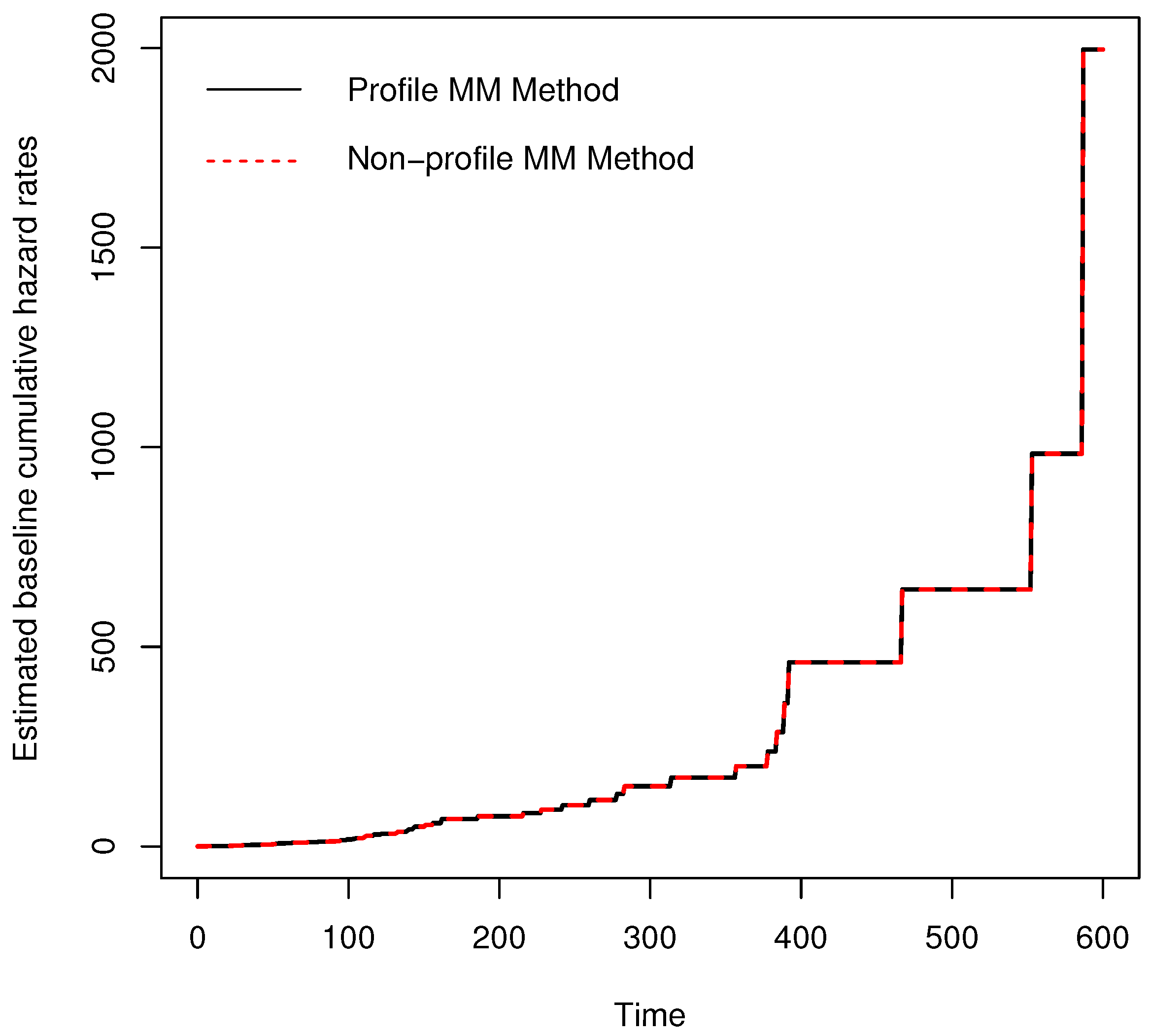
6. Real Data Analysis

We apply our methods to the Veterans’ administration lung cancer study data with sample size 137, and the number of covariate is 8. The data can be retrieved from the R package “survival” and the information for the covariates are given in

Table 8. Covariates of lung cancer data.

Covariate	Detailed Description
Trt	treatment, 1 = Standard 2 = test
Celltype	Squamous, smallcell, adeno, large
Time	Survival time
Status	Censoring status
Karno	Karnofsky performance score (100 = good)
Diagtime	Months from diagnosis to randomisation
Age	In years
Prior	Prior therapy (0 = no, 10 = yes)

.

This dataset is generally applied for the illustration of the proportional odds model. For the purpose of comparing against other studies, we use the data of patient with no prior therapy where the censoring rate is 6.19% and the covariates are “celltype” and “karno”. Two MM algorithms are applied to estimate the parameters. Moreover, the standard deviation is estimated by 1000 times of bootstraps, where ${\widehat{\beta }}_g^{\ast },g=1,\dots ,G$ is the estimate of $g^{th}$ bootstrap. We construct the $100(1-\alpha )\%$ confidence interval of $\mathit{\beta }$ using normal approximation.

$$\left({\overline{\mathit{\beta }}}^{\ast }\pm z_{\alpha /2}{\widehat{\mathrm{se}}}^{\ast }(\widehat{\mathit{\beta }})\right),$$

(12)

where ${\overline{\mathit{\beta }}}^{\ast }=(1/G){\displaystyle \sum _{g=1}^G}{\widehat{\mathit{\beta }}}_g^{\ast }$ and

$${\widehat{\mathrm{se}}}^{\ast }\left(\widehat{\mathit{\beta }}\right)=\sqrt{(1/(G-1)){\displaystyle \sum _{g=1}^G}{\left({\widehat{\mathit{\beta }}}_g^{\ast }-{\overline{\mathit{\beta }}}^{\ast }\right)}^2}$$

(13)

bootstrap confidence interval of $100(1-\alpha )\%$ is

$$\left({\widehat{\mathit{\beta }}}_L^{\ast },{\widehat{\mathit{\beta }}}_U^{\ast }\right),$$

(14)

where ${\widehat{\mathit{\beta }}}_L^{\ast }$ and ${\widehat{\mathit{\beta }}}_U^{\ast }$ denotes the quantile of $\left\{{\widehat{\mathit{\beta }}}_1^{\ast },\dots ,{\widehat{\mathit{\beta }}}_G^{\ast }\right\}$’s $\alpha /2$ and $1-\alpha /2$ separately.

Table 9. The estimation result from profile MM method.

Variable	MLE	SE	CI1	CI2
karno	−0.0532	0.0105	[−0.0741,−0.0329]	[−0.0714,−0.0363]
squamous vs. large	−0.1814	0.6382	[−1.4255,1.0761]	[−1.2761,0.8135]
small vs. large	1.3827	0.4816	[0.4820,2.3699]	[0.6734,2.2438]
adenovs large	1.3138	0.4691	[0.4521,2.2910]	[0.6341,2.1755]

and

Table 10. The estimation result from non-profile MM method.

Variable	MLE	SE	CI1	CI2
karno	−0.0532	0.0106	[−0.0746,−0.0329]	[−0.0722,−0.0377]
squamous vs. large	−0.1814	0.6589	[−1.4696,1.1134]	[−1.2175,0.8777]
small vs. large	1.3827	0.5105	[0.4431,2.4442]	[0.6459,2.2644]
adeno vs. large	1.3138	0.4659	[0.4654,2.2919]	[0.6267,2.1613]

present the estimation result of two MM algorithms, where the standard estimated error (SE) is defined by Equation (13) and the 95% confidence interval (CI1) is defined by Equation (12). Moreover, the 95% confidence interval (CI2) is defined by Equation (14). In addition, the estimated cumulative hazard function are plotted in Figure 3.

From Table 9 and Table 10, for the same patient, every increase of 1 degree of “karno”, the decrease in possibility of death is $exp(-0.0532)=0.9482$. From Figure 3, the estimation results of the baseline cumulative hazard function of two MM methods are almost the same. We can find that our method produces a similar result, as concluded by [3], and is a little bit different from the result presented by [5,7,11], which is shown by

Table 11. Estimation result from other studies.

Variable	(Bennett [3])	(Pettitt [5])	(Murphy et al. [7])	(Lam & Leung [11])
karno	−0.053	−0.055	−0.055	−0.053
squamous vs. large	−0.181	−0.177	−0.217	−0.247
small vs. large	1.383	1.438	1.440	1.367
adeno vs. large	1.314	1.302	1.339	1.316

from [11].

Then, we consider all eight covariates for model fitting where the censoring rate is 6.57%. We first use the method from Section 4.1 to estimate the parameters. After obtaining the estimation results, we apply the SCAD and MCP penalties discussed in Section 4.2 for parameter selection, and the result is presented by

Table 12. The result of variable selection for lung cancer data.

Variable	Profile MM			Non-Profile MM
	MLE	SCAD	MCP	MLE	SCAD	MCP
trt	−0.0141	0	0	−0.0141	0	0
squamous vs. large	−0.0348	0	0	−0.0348	0	0
small vs. large	1.2412	1.1960	1.1944	1.2412	1.1873	1.1859
adeno vs. large	1.3251	1.3653	1.3670	1.3250	1.3596	1.3593
karno	−0.0597	−0.0582	−0.0590	−0.0597	−0.0589	−0.0590
diagtime	−0.0025	0	0	−0.0025	0	0
age	−0.0141	0	0	−0.0141	0	0
prior	−0.1663	0	0	−0.1663	0	0

.

From Table 12, the Profile MM method and Non-profile MM method produce similar results. Without considering the penalties, the results of parameter separated MM algorithms demonstrate that four parameters including “small vs. large”, “adeno vs. large”, “karno” and “prior” significantly affect the death rate. After introducing the penalties, we conduct the variable selection and 5 covariates are shrunk to 0. Only three significant parameters are preserved, which are “small vs. large”, “adeno vs. large” and “karno”. “small vs. large” and “adeno vs. large” lead to a positive effect to the death rate while “karno” is negatively related to the death rate, which is in line with the common sense in reality.

7. Conclusions and Future Work

The proportional odds models are more competitive than proportional hazards models in dealing with right-censored survival data, where mortality tends to be uniform over time. The MM algorithm has the advantages of simple structure, strong interpretability and easy implementation. Hence, it is a useful tool for optimization problems and has a broad range of applications in statistics. In this work, we introduce the MM algorithm into the estimation of the proportional odds model. We first develop two MM algorithms for the estimation of proportional odds models, which greatly simplify the estimation process by constructing two simple surrogate functions for the log-likelihood function. The proposed MM algorithms successfully separate the parameters and decompose the high-dimensional maximization into separated low-dimensional ones, which may avoid the matrix inversion and can be used to more general scenarios. Moreover, we apply the MM methods to the regularized estimation in sparse high-dimensional proportional odds regression models with SCAD and MCP penalties. We find that the proposed MM algorithms with the property of separating parameters can mesh well with the SCAD and MCP penalties, which yield good results in simultaneous parameter estimation and variable selection.

The advantage of our algorithm is that we separate the estimation of the baseline hazard and other parameters, which makes the estimation process more efficient. In future studies, such technique derived from the semi-parametric model can be further extended to the application of parameter estimation for fully non-parametric models. In addition, as we mentioned in previous sections, the existing methods for the proportional odds model with right censored data involve high computation complexity when dealing with high-dimensional data. However, our proposed algorithm can help to avoid matrix inversion, which is capable of high-dimensional regression analysis. Furthermore, the advantage of our algorithm is that it can mesh well with the existing quasi-Newton acceleration and other simple off-the-shelf accelerators to further boost the estimation process. Although our proposed MM algorithms are developed for the proportional odds models, a parallel approach can essentially be developed for the more general transformation models. We will investigate this in our future work.

References

1. McCullagh, P. A logistic model for paired comparisons with ordered categorical data. Biometrika 1977, 64, 449–453. [Google Scholar] [CrossRef]
2. McCullagh, P. Regression models for ordinal data. J. R. Stat. Soc. Ser. B 1980, 42, 109–127. [Google Scholar] [CrossRef]
3. Bennett, S. Analysis of survival data by the proportional odds model. Stat. Med. 1983, 2, 273–277. [Google Scholar] [CrossRef] [PubMed]
4. Bennett, S. Log-logistic regression models for survival data. J. R. Stat. Soc. Ser. C 1983, 32, 165–171. [Google Scholar] [CrossRef]
5. Pettitt, A. Proportional odds models for survival data and estimates using ranks. J. R. Stat. Soc. Ser. C 1984, 33, 169–175. [Google Scholar] [CrossRef]
6. Rossini, A.; Tsiatis, A. A semiparametric proportional odds regression model for the analysis of current status data. J. Am. Stat. Assoc. 1996, 91, 713–721. [Google Scholar] [CrossRef]
7. Murphy, S.; Rossini, A.; van der Vaart, A.W. Maximum likelihood estimation in the proportional odds model. J. Am. Stat. Assoc. 1997, 92, 968–976. [Google Scholar] [CrossRef]
8. Huang, J.; Rossini, A. Sieve estimation for the proportional-odds failure-time regression model with interval censoring. J. Am. Stat. Assoc. 1997, 92, 960–967. [Google Scholar] [CrossRef]
9. Shen, X. Propotional odds regression and sieve maximum likelihood estimation. Biometrika 1998, 85, 165–177. [Google Scholar] [CrossRef]
10. Rabinowitz, D.; Betensky, R.A.; Tsiatis, A.A. Using conditional logistic regression to fit proportional odds models to interval censored data. Biometrics 2000, 56, 511–518. [Google Scholar] [CrossRef]
11. Lam, K.; Leung, T. Marginal likelihood estimation for proportional odds models with right censored data. Lifetime Data Anal. 2001, 7, 39–54. [Google Scholar] [CrossRef] [PubMed]
12. Hunter, D.R.; Lange, K. Computing estimates in the proportional odds model. Ann. Inst. Stat. Math. 2002, 54, 155–168. [Google Scholar] [CrossRef]
13. Royston, P.; Parmar, M.K. Flexible parametric proportional-hazards and proportional-odds models for censored survival data, with application to prognostic modelling and estimation of treatment effects. Stat. Med. 2002, 21, 2175–2197. [Google Scholar] [CrossRef]
14. Banerjee, S.; Dey, D.K. Semiparametric proportional odds models for spatially correlated survival data. Lifetime Data Anal. 2005, 11, 175–191. [Google Scholar] [CrossRef]
15. Wang, L.; Dunson, D.B. Semiparametric Bayes’ proportional odds models for current status data with underreporting. Biometrics 2011, 67, 1111–1118. [Google Scholar] [CrossRef]
16. Lin, X.; Wang, L. Bayesian proportional odds models for analyzing current status data: Univariate, clustered, and multivariate. Commun. Stat.-Simul. Comput. 2011, 40, 1171–1181. [Google Scholar] [CrossRef]
17. Augustin, N.H.; Kim, S.W.; Uhlig, A.; Hanser, C.; Henke, M.; Schumacher, M. A flexible multivariate random effects proportional odds model with application to adverse effects during radiation therapy. Biom. J. 2017, 59, 1339–1351. [Google Scholar] [CrossRef]
18. Bao, Y.; Vicente Garibay, C.; Francisco, L.; Adriano Kamimura, S. Cure rate proportional odds models with spatial frailties for interval-censored data. Commun. Stat. Appl. Methods 2017, 24, 605–625. [Google Scholar] [CrossRef]
19. Kumar, D.; Sankaran, P. Proportional odds model—A quantile approach. J. Appl. Stat. 2019, 46, 1937–1955. [Google Scholar] [CrossRef]
20. Chen, J.; Terrell, G.R.; Kim, I.; Daviglus, M.L. Proportional odds model with log-concave density estimation. Stat. Sin. 2020, 30, 877–901. [Google Scholar] [CrossRef]
21. Wang, L.; Wang, L. Regression analysis of arbitrarily censored survival data under the proportional odds model. Stat. Med. 2021, 40, 3724–3739. [Google Scholar] [CrossRef] [PubMed]
22. Zhu, L.; Tong, X.; Cai, D.; Li, Y.; Sun, R.; Srivastava, D.K.; Hudson, M.M. Maximum likelihood estimation for the proportional odds model with mixed interval-censored failure time data. J. Appl. Stat. 2021, 48, 1496–1512. [Google Scholar] [CrossRef] [PubMed]
23. Wang, L.; Wang, L. An EM algorithm for analyzing right-censored survival data under the semiparametric proportional odds model. Commun. Stat. Theory Methods 2020, 51, 5284–5297. [Google Scholar] [CrossRef]
24. Tibshirani, R. The lasso method for variable selection in the Cox model. Stat. Med. 1997, 16, 385–395. [Google Scholar] [CrossRef]
25. Fan, J.; Li, R. Variable selection for Cox’s proportional hazards model and frailty model. Ann. Stat. 2002, 30, 74–99. [Google Scholar] [CrossRef]
26. Zou, H. A note on path-based variable selection in the penalized proportional hazards model. Biometrika 2008, 95, 241–247. [Google Scholar] [CrossRef]
27. Lu, W.; Zhang, H.H. Variable selection for proportional odds model. Stat. Med. 2007, 26, 3771–3781. [Google Scholar] [CrossRef]
28. Hunter, D.R.; Lange, K. Quantile regression via an MM algorithm. J. Comput. Graph. Stat. 2000, 9, 60–77. [Google Scholar]
29. Hunter, D.R. MM algorithms for generalized Bradley-Terry models. Ann. Stat. 2004, 32, 384–406. [Google Scholar] [CrossRef]
30. Zhou, H.; Lange, K. MM algorithms for some discrete multivariate distributions. J. Comput. Graph. Stat. 2010, 19, 645–665. [Google Scholar] [CrossRef]
31. Tian, G.L.; Ding, X.; Liu, Y.; Tang, M.L. Some new statistical methods for a class of zero-truncated discrete distributions with applications. Comput. Stat. 2019, 34, 1393–1426. [Google Scholar] [CrossRef]
32. Hunter, D.R.; Li, R. Variable selection using MM algorithms. Ann. Stat. 2005, 33, 1617–1642. [Google Scholar] [CrossRef] [PubMed]
33. Nguyen, H.D.; McLachlan, G.J. Maximum likelihood estimation of Gaussian mixture models without matrix operations. Adv. Data Anal. Classif. 2015, 9, 371–394. [Google Scholar] [CrossRef]
34. Huang, X.; Xu, J.; Tian, G. On profile MM algorithms for gamma frailty survival models. Stat. Sin. 2019, 29, 895–916. [Google Scholar] [CrossRef]
35. Fan, J.; Li, R. Variable selection via nonconcave penalized likelihood and its oracle properties. J. Am. Stat. Assoc. 2001, 96, 1348–1360. [Google Scholar] [CrossRef]
36. Zhang, C.H. Nearly unbiased variable selection under minimax concave penalty. Ann. Stat. 2010, 38, 894–942. [Google Scholar] [CrossRef]
37. Schwarz, G. Estimating the dimension of a model. Ann. Stat. 1978, 6, 461–464. [Google Scholar] [CrossRef]
38. Benjamini, Y.; Hochberg, Y. Controlling the false discovery rate: A practical and powerful approach to multiple testing. J. R. Stat. Soc. Ser. B 1995, 57, 289–300. [Google Scholar] [CrossRef]
Figure 1. True and estimated baseline cumulative functions with different censoring rate when sample size is 250. The solid and dotted lines plot the true and estimated baseline cumulative hazard functions, respectively. The estimated baseline cumulative hazard function is the empirical average of the estimated baseline cumulative hazard functions based on 500 replications.
Mathematics 10 03362 g001
Figure 2. True and estimated baseline cumulative functions with different sample size when censoring rate is 50%. The solid and dotted lines plot the true and estimated baseline cumulative hazard functions, respectively. The estimated baseline cumulative hazard function is the empirical average of the estimated baseline cumulative hazard functions based on 500 replications.
Mathematics 10 03362 g002
Figure 3. Estimated baseline cumulative functions for lung cancer data.
Mathematics 10 03362 g003