Partial Learning Using Partially Explicit Discretization for Multicontinuum/Multiscale Problems with Limited Observation: Dual Continuum Heterogeneous Poroelastic Media Simulation

Abstract

In this paper, we consider the poroelasticity problem in heterogeneous media. The mathematical model is described by a coupled system of equations for displacement and pressure in the coupled dual continuum porous media. We propose a new method based on hybrid explicit–implicit (HEI) learning to solve the poroelasticity problem in dual continuum heterogeneous media. We use a finite element method with standard linear basis functions for spatial approximation. We apply the explicit–implicit time scheme, where the explicit scheme is used for the low-conductive continuum and the implicit scheme for the high-conductive. The fixed-strain splitting scheme is used to accelerate the computation and decouple the flow and mechanics problems. The main idea of the proposed method is partial learning of particular degrees of freedom of the high-conductive continuum’s pressure (implicit part of the flow). First, we train a deep neural network (DNN) to obtain values of the implicit part of the flow at some spatial points at some time moments. Then, we apply the Discrete Empirical Interpolation Method (DEIM) combined with Proper Orthogonal Decomposition (POD) to restore the complete implicit parts and perform linear interpolation over time. Consequently, we treat the high-conductive continuum’s pressure as a known function and use it to find the other continuum’s pressure and displacements. Numerical results for the two-dimensional model problem are presented. The results demonstrate that the proposed method provides fast and accurate predictions.

1. Introduction

Accurately describing the stress–strain state of poroelastic bodies is an urgent and essential problem for deformable solid mechanics [1,2,3]. The mathematical model consists of equations for pressure and displacements. The most important feature of the model is that the equations are coupled. Modern computational technology allows us to solve such problems using various numerical methods. Among them, it is necessary to highlight the finite element and finite difference methods. The finite element method is best suited for spatial approximation of a problem given in a complex domain. At the same time, the finite difference method is commonly used for time approximation.

The most important classification of the finite difference schemes for time approximation is related to their assignment as explicit or implicit ones [4,5,6]. Implicit schemes are popular in numerical simulation due to their excellent stability, which does not depend on spatial mesh size, time step size, and conductivity. However, these schemes are computationally expensive. In addition, they do not always correctly describe the behavior of the solution. When using implicit schemes, in a sense, we remove high frequencies. On the other hand, explicit schemes are computationally efficient and can capture the solution’s dynamics. However, they have conditional stability depending on the grid size, time step size, and conductivity. Therefore, it makes sense in multicontinuum problems to use a combination of explicit and implicit schemes, often called an explicit–implicit or partially explicit scheme. In this combination, we use an implicit scheme for a high-conductivity continuum and an explicit scheme for a low-conductivity continuum.

Another important detail related to time approximation is the use of splitting schemes. When solving systems of partial differential equations numerically, we can use either a coupled scheme or splitting schemes. In the coupled scheme, we solve all the equations at the same time. In splitting schemes, the transition to a new temporal layer is carried out by sequential solution of separate equations. The splitting schemes simplify the construction of difference schemes and reduce required computational resources. For poroelasticity problems, one can note drained, undrained, fixed-strain, fixed-stress, and weighted splitting schemes [7,8,9,10].

The above schemes help solve poroelasticity problems in the most computationally efficient way. They all refer in one way or another to temporal approximation. However, there are other ways to speed up computations. For example, one can use numerical homogenization and multiscale methods [11,12,13,14]. These methods allow us to solve problems in heterogeneous media using coarse grids, thereby significantly reducing the size of the discrete problem. It is worth noting that one can combine these methods with machine learning to accelerate some steps [14].

Note that one can encounter an issue related to a limited number of possible observation points in applied poroelasticity problems. For example, it can be some measurement devices. The problem of reconstructing the overall picture from the limited observation arises in such situations. Unfortunately, classical spatial interpolation methods cannot give an accurate approximation. For such cases, it is better to use the Discrete Empirical Interpolation Method (DEIM) [15] with Proper Orthogonal Decomposition (POD) [16,17]. POD is a global model reduction method. The method’s main idea is to find the most energetic modes and use them as basis functions. These basis functions form the projection basis matrix. The DEIM provides an algorithm for finding interpolation indices (points) and the POD’s solution degrees of freedom. One can restore the required function by using the function’s values at these interpolation indices and the projection basis matrix.

This paper proposes a new method based on hybrid explicit–implicit (HEI) learning [18] to solve the poroelasticity problem in dual continuum heterogeneous media. In this model, we introduce a pressure field for each continuum, and the effective stress contains each continuum’s part in the equation for mechanical deformations [19,20,21,22]. We use a finite element method with standard linear basis functions for spatial approximation. We apply the explicit–implicit time scheme, where the explicit scheme is used for the low-conductive continuum and the implicit scheme for the high-conductive one. Furthermore, the fixed-strain splitting scheme is used to accelerate computation. The main idea of the proposed method is partial learning of particular degrees of freedom of the high-conductive continuum’s pressure (implicit part of the flow). First, we train a deep neural network (DNN) to obtain values of the implicit part of the flow at some spatial points at some time moments. Then, we apply the DEIM with POD to restore the complete implicit parts and perform linear interpolation over time. Consequently, we treat the high-conductive continuum’s pressure as a known function and use it to find the other continuum’s pressure and displacements. Our method consists of two stages: offline and online. First, in the offline stage, we generate the POD basis projection matrix, define interpolation indices, and train DNN. Then, we solve the poroelasticity problem by treating the implicit part of the flow as a known function in the online stage.

Offline stage

1

Construct the POD projection basis matrix and define the interpolation points using DEIM.

2

Generate the training dataset.

•

Generate the input data.

•

Solve the poroelasticity problem with the partially explicit discretization at each time step.

3

Train the Deep Neural Network to obtain values of the implicit flow part at the interpolation points at some time steps.

Online stage

1

The Deep Neural Network obtains the implicit part of the pressure at the interpolation points at some time moments.

2

The POD projection basis matrix restores the complete implicit parts of the flow at some time moments.

3

Linear interpolation over time.

4

For each time step,

•

Compute the explicit flow part using the learned and interpolated implicit one.

•

Solve the displacement using the implicit and explicit parts of the flow.

The work has the following structure. First, we present the mathematical model in Section 2 and its approximation in Section 3. Then, Section 3 describes the Discrete Empirical Interpolation Method with Proper Orthogonal Decomposition. Section 4 presents our partial learning partially explicit discretization approach. Next, we present numerical results for two-dimensional model poroelasticity problems in the dual continuum heterogeneous medium in Section 5. Finally, Section 6 summarizes the work.

2. Problem Formulation

Let $\Omega \subset {\mathbb{R}}^d$ be a computational domain, where d denotes a geometrical dimension of the problem and equals 2 for a two-dimensional case. We consider a dual continuum model, where the first continuum is high-conductive, and the second continuum is low-conductive. The mathematical model is described by a coupled system of equations for pressures $p_1$, $p_2$ and displacements u [23,24]

$$\begin{array}{cc}\hfill & {\alpha }_1\frac{\partial \mathrm{div}u}{\partial t}+\frac{1}{M_1}\frac{\partial p_1}{\partial t}-\mathrm{div}\left(k_1\mathrm{grad}{p}_1\right)+r_{12}(p_1-p_2)=0,x\in \Omega ,\hfill \\ \hfill & {\alpha }_2\frac{\partial \mathrm{div}u}{\partial t}+\frac{1}{M_2}\frac{\partial p_2}{\partial t}-\mathrm{div}\left(k_2\mathrm{grad}{p}_2\right)-r_{21}(p_1-p_2)=g,x\in \Omega ,\hfill \\ \hfill & -\mathrm{div}\sigma \left(u\right)+{\alpha }_1\mathrm{grad}{p}_1+{\alpha }_2\mathrm{grad}{p}_2=0,x\in \Omega ,\hfill \end{array}$$

(1)

where $k_{\alpha }={\kappa }_{\alpha }/\mu$, ${\kappa }_1$ and ${\kappa }_2$ are the permeabilities, g is the source term, ${\alpha }_1$ and ${\alpha }_2$ are the Biot coefficients, $M_1$ and $M_2$ are the Biot moduli, $r_{mf}$ is the transfer term between continua, $\mu$ is the fluid viscosity, u is the displacement, and $\sigma$ is the stress tensor.

The relation between the stress and strain tensors is given as

$$\sigma \left(u\right)=2\mu \epsilon \left(u\right)+\lambda \mathrm{div}u\mathcal{I},\epsilon \left(u\right)=\frac{1}{2}(\mathrm{grad}u+\mathrm{grad}{u}^T),$$

where $\epsilon$ is the strain tensor, and $\lambda$ and $\mu$ are the Lamé coefficients.

We consider a system of Equation (1) with the following initial conditions

$$\begin{array}{cc}\hfill & p_1\left(0\right)=p_2\left(0\right)=p_0,x\in \Omega ,\hfill \\ \hfill & u\left(0\right)=u_0,x\in \Omega ,\hfill \end{array}$$

(2)

and boundary conditions

$$\begin{array}{cc}\hfill & -k_1\frac{\partial p_1}{\partial n}=0,x\in \partial \Omega ,-k_2\frac{\partial p_2}{\partial n}=0,x\in \partial \Omega ,\hfill \\ \hfill & u_1=0,{\left(\sigma n\right)}_2=0,x\in {\Gamma }_L\cup {\Gamma }_R,u_2=0,{\left(\sigma n\right)}_1=0,x\in {\Gamma }_T\cup {\Gamma }_B\hfill \end{array}$$

(3)

where boundaries ${\Gamma }_L\cup {\Gamma }_R\cup {\Gamma }_T\cup {\Gamma }_B=\partial \Omega$; ${\Gamma }_L$, ${\Gamma }_R$, ${\Gamma }_B$, ${\Gamma }_T$ denote the left, right, bottom, and top boundaries, respectively.

3. Approximation

Variational formulation. For spatial approximation of the system of Equation (1) with boundary conditions (3), we use a finite element method. We define the following functional spaces

$$W_1=W_2=H^1(\Omega ),$$

$$V=\{v\in {\left[H^1(\Omega )\right]}^d:v_1=0\mathrm{on}{\Gamma }_L\cup {\Gamma }_R\mathrm{and}{v}_2=0\mathrm{on}{\Gamma }_T\cup {\Gamma }_B\}.$$

The variational formulation of the poroelasticity problem can be written as follows. Find $(p_1,p_2,u)\in W_1\times W_2\times V$ such that

$$\begin{array}{cc}\hfill & d_1\left(\frac{\partial u}{\partial t},w_1\right)+c_1\left(\frac{\partial p_1}{\partial t},w_1\right)+b_1(p_1,w_1)+q_{12}(p_1-p_2,w_1)=0,\forall w_1\in W_1,\hfill \\ \hfill & d_2\left(\frac{\partial u}{\partial t},w_2\right)+c_2\left(\frac{\partial p_2}{\partial t},w_2\right)+b_2(p_2,w_2)-q_{21}(p_1-p_2,w_2)=l\left(w_2\right),\forall w_2\in W_2,\hfill \\ \hfill & a(u,v)+g_1(p_1,v)+g_2(p_2,v)=0,\forall v\in V,\hfill \end{array}$$

(4)

where the bilinear and linear forms are the following

$$b_1(p_1,w_1)={\int }_{\Omega }{k}_1\mathrm{grad}{p}_1·\mathrm{grad}{w}_{1}dx,b_2(p_2,w_2)={\int }_{\Omega }{k}_2\mathrm{grad}{p}_2·\mathrm{grad}{w}_{2}dx$$

$$c_1(p_1,w_1)={\int }_{\Omega }\frac{1}{M_1}{p}_1{w}_{1}dx,c_2(p_2,w_2)={\int }_{\Omega }\frac{1}{M_2}{p}_2{w}_{2}dx,l\left(w_2\right)={\int }_{\Omega }g{w}_{2}dx,$$

$$q_{12}(p_1-p_2,w_1)={\int }_{\Omega }{r}_{12}(p_1-{\Pi }_{21}{p}_2)w_{1}dx,q_{21}(p_1-p_2,w_2)={\int }_{\Omega }{r}_{21}({\Pi }_{12}{p}_1-p_2)w_{2}dx,$$

$$d_1(u,w_1)={\int }_{\Omega }{\alpha }_1\mathrm{div}u{w}_{1}dx,d_2(u,w_2)={\int }_{\Omega }{\alpha }_2\mathrm{div}u{w}_{2}ds,a(u,v)={\int }_{\Omega }\mathsf{\sigma }\left(u\right):\mathsf{\epsilon }\left(v\right)dx,$$

$$g_1(p_1,v)={\int }_{\Omega }{\alpha }_1\mathrm{grad}{p}_1·vdx,g_2(p_2,v)={\int }_{\Omega }{\alpha }_2\mathrm{grad}{p}_2·vdx,$$

where ${\Pi }_{12}$ is the projection operator from $W_1$ to $W_2$ defined as

$${\int }_{\gamma }({\Pi }_{12}{p}_1-p_1)w_{2}ds=0,\forall w_2\in W_2.$$

and ${\Pi }_{21}={\Pi }_{12}^{*}$ (see [25] for details).

Discretization in time. We use an explicit–implicit scheme for the time approximation, where the explicit scheme is used for the low-conductive continuum and the implicit scheme for the high-conductive one. Let $u^n=u(x,t^n)$, $p_1^n=p_1(x,t^n)$, $p_2^n=p_2(x,t^n)$, and $t^n=n\tau$, where $\tau =T/N_t$ is the time step size, T is the final time, and $N_t$ is the count of time steps. Then, the problem can be formulated as follows. For $n=0,\cdots ,N_t-1$, find $(p_1^{n+1},p_2^{n+1},u^{n+1})\in (W_1\times W_2\times V)$ such that

$$\begin{array}{cc}\hfill & d_1\left(\frac{u^{n+1}-u^n}{\tau },w_1\right)+c_1\left(\frac{p_1^{n+1}-p_1^n}{\tau },w_1\right)+b_1(p_1^{n+1},w_1)+q_{12}(p_1^{n+1}-p_2^{n+1},w_1)=0,\hfill \\ \hfill & d_2\left(\frac{u^{n+1}-u^n}{\tau },w_2\right)+c_2\left(\frac{p_2^{n+1}-p_2^n}{\tau },w_2\right)+b_2(p_2^n,w_2)-q_{21}(p_1^{n+1}-p_2^{n+1},w_2)=l\left(w_2\right),\hfill \\ \hfill & a(u^{n+1},v)+g_1(p_1^{n+1},v)+g_2(p_2^{n+1},v)=0,\forall vs.\in V,\hfill \end{array}$$

(5)

where $\forall (w_1,w_2,v)\in (W_1,W_2,V)$.

Splitting scheme. We can solve the poroelasticity problem using the fixed-strain splitting scheme. The fixed-strain splitting scheme decouples the flow and mechanics system solving them sequentially at each time step. Then, we have the following problem formulation. For $n=1,\cdots N_t-1$, find

• Pressures $(p_1^{n+1},p_2^{n+1})\in (W_1\times W_2)$ such that

  $$\begin{array}{cc}\hfill & d_1\left(\frac{u^n-u^{n-1}}{\tau },w_1\right)+c_1\left(\frac{p_1^{n+1}-p_1^n}{\tau },w_1\right)+b_1(p_1^{n+1},w_1)+q_{12}(p_1^{n+1}-p_2^{n+1},w_1)=0,\hfill \\ \hfill & d_2\left(\frac{u^n-u^{n-1}}{\tau },w_2\right)+c_2\left(\frac{p_2^{n+1}-p_2^n}{\tau },w_2\right)+b_2(p_2^n,w_2)-q_{21}(p_1^{n+1}-p_2^{n+1},w_2)=l\left(w_2\right),\hfill \end{array}$$

  (6)

  where $\forall (w_1,w_2)\in (W_1,W_2)$.
• Displacements $u^{n+1}$ such that

  $$a(u^{n+1},v)+g_1(p_1^{n+1},v)+g_2(p_2^{n+1},v)=0,$$

  (7)

  where $\forall vs.\in V$.

Discrete formulation. Let ${\mathcal{T}}^h$ be a grid partition of the computational domain $\Omega$ into finite elements and $W_{1,h}\subset W_1$, $W_{2,h}\subset W_2$ and $V_h\subset V$ be the finite element subspaces on ${\mathcal{T}}^h$.

$$u=\sum u_i{\Phi }_i,p_1=\sum p_{1,i}{\varphi }_{1,i}{p}_2=\sum p_{2,i}{\varphi }_{2,i}$$

(8)

where $\Phi$, ${\varphi }_1$, and ${\varphi }_2$ are the linear basis functions defined on ${\mathcal{T}}^h$.

The discrete formulation of the poroelasticity problem using the explicit–implicit time scheme will have the following form for coupled and splitting schemes.

Coupled scheme. For $n=0,\cdots ,N_t-1,$ find $(p_1^{n+1},p_2^{n+1},u^{n+1})$ such that

$$\begin{array}{cc}\hfill & B_1{p}_1^{n+1}+C_1\frac{p_1^{n+1}-p_1^n}{\tau }+D_1\frac{u^{n+1}-u^n}{\tau }+Q_{12}(p_1^{n+1}-p_2^{n+1})=0,\hfill \\ \hfill & B_2{p}_2^n+C_2\frac{p_2^{n+1}-p_2^n}{\tau }+D_2\frac{u^{n+1}-u^n}{\tau }-Q_{21}(p_1^{n+1}-p_2^{n+1})=L,\hfill \\ \hfill & A{u}^{n+1}+G_1{p}_1^{n+1}+G_2{p}_2^{n+1}=0.\hfill \end{array}$$

(9)

where

$$B_1=[b_1,ij],b_{1,ij}=b_1({\varphi }_{1,j},{\varphi }_{1,i}),B_2=[b_2,ij],b_{2,ij}=b_1({\varphi }_{2,j},{\varphi }_{2,i}),$$

$$C_1=[c_1,ij],c_{1,ij}=c_1({\varphi }_{1,j},{\varphi }_{1,i}),C_2=[c_2,ij],c_{2,ij}=c_2({\varphi }_{2,j},{\varphi }_{2,i}),$$

$$D_1=[d_1,ij],d_{1,ij}=d_1({\Phi }_j,{\varphi }_{1,i}),D_2=[d_2,ij],d_{2,ij}=d_2({\Phi }_j,{\varphi }_{2,i}),$$

$$Q_{12}=[q_{12},ij],q_{12,ij}=q_{12}({\varphi }_{1,j},{\varphi }_{1,i}),Q_{21}=[q_{21},ij],q_{21,ij}=q_{21}({\varphi }_{2,j},{\varphi }_{2,i}),$$

$$G_1=[g_1,ij],g_{1,ij}=g_1({\varphi }_j,{\Phi }_{1,i}),G_2=[g_2,ij],g_{2,ij}=g_2({\varphi }_j,{\Phi }_{2,i}),$$

$$L=[l,i],l_i=l_{(}{\varphi }_{2,i}),A_u=[a_u,ij],a_{u,ij}=a_u({\Phi }_j,{\Phi }_i).$$

For $n=1,\cdots ,N_t-1,$ find

• Pressures $(p_1^{n+1},p_2^{n+1})$ such that

  $$\begin{array}{cc}\hfill & B_1{p}_1^{n+1}+C_1\frac{p_1^{n+1}-p_1^n}{\tau }+D_1\frac{u^n-u^{n-1}}{\tau }+Q_{12}(p_1^{n+1}-p_2^{n+1})=0,\hfill \\ \hfill & B_2{p}_2^n+C_2\frac{p_2^{n+1}-p_2^n}{\tau }+D_2\frac{u^n-u^{n-1}}{\tau }-Q_{21}(p_1^{n+1}-p_2^{n+1})=L.\hfill \end{array}$$

  (10)
• Displacements $u^{n+1}$ such that

  $$A{u}^{n+1}+G_1{p}_1^{n+1}+G_2{p}_2^{n+1}=0.$$

  (11)

In the next section, we will consider the Discrete Empirical Interpolation Method we will use for our partial learning approach.

4. Discrete Empirical Interpolation Method with Proper Orthogonal Decomposition

When we need to reconstruct the solution in a heterogeneous medium as accurately as possible using only several points, we cannot apply the classical spatial interpolation methods. The Discrete Empirical Interpolation Method (DEIM) is better suited for such situations. The procedure of such spatial interpolation consists of the following steps:

• Computing the Proper Orthogonal Decomposition (POD) basis functions;
• Determining the interpolation nodes using the DEIM algorithm.

In our work, we want to use the DEIM to spatially interpolate the pressure of the high-conductive continuum. In this case, after we train the neural network to acquire values at several points, we can reconstruct the pressure in the whole area.

Computing the Proper Orthogonal Decomposition (POD) basis functions. To compute snapshot functions, we save the first continuum’s pressure data into matrix B with every second time step in each row saved, solving the problem five times with different parametric functions. Thus, we obtain a matrix B with $N_s$ by M elements:

$$B=\left(\begin{array}{cccc}{a}_{1,1}& a_{1,2}& \cdots & a_{1,N_s}\\ a_{2,1}& a_{2,2}& \cdots & a_{2,N_s}\\ ⋮& ⋮& \ddots & ⋮\\ a_{M,1}& a_{M,2}& \cdots & a_{M,N_s}\end{array}\right),$$

where $N_s$ is the number of snapshots, and M is the number of degrees of freedom (mesh nodes in our case).

Next, we assemble a symmetric positive covariance matrix of dimension $M\times M$.

$$R=B{B}^T$$

Then, we determine eigenvalues ${\lambda }_k$ and eigenvectors ${\psi }_k$ in matrix R. We sort the eigenvalues in descending order ${\lambda }_1>{\lambda }_2>\cdots >{\lambda }_m>\cdots$.

Finally, we choose m eigenvectors ${\psi }_k$ corresponding to the first m eigenvalues ${\lambda }_k$ ($m\ll M$). These eigenvectors will be our basis functions.

Determining the interpolation nodes using the DEIM algorithm. After calculating the basis functions, we can represent the desired function (in our case, $p_1$) in the following form.

$$p_1\approx \Psi c,$$

(12)

where $p_1={(p_{1,1},\cdots ,p_{1,M})}^T$, $\Psi =({\psi }_1,\cdots ,{\psi }_m)$, $c={(c_1,\cdots ,c_m)}^T$.

To determine $p_1$, we need to know c. Note that we can find c using m rows. Suppose we can know the values of $p_1$ in any m nodes (rows). In this case, our task is to determine m optimal nodes (rows). We achieve this using the DEIM algorithm [15].

The DEIM finds m distinct interpolation nodes $(v_1,\cdots ,v_m)$ and assembles the DEIM interpolation nodes matrix $P=(e_{n_1},\cdots ,e_{n_m})$, where $e_{n_i}$ is the $n_i$-th column of the identity matrix $I_M$. After that, we can restore $p_1$ as follows.

$$p_1\approx \Psi {(P^T\Psi )}^{-1}{P}^T{p}_1,$$

(13)

where $P^T{p}_1$ samples $p_1$ at m components only.

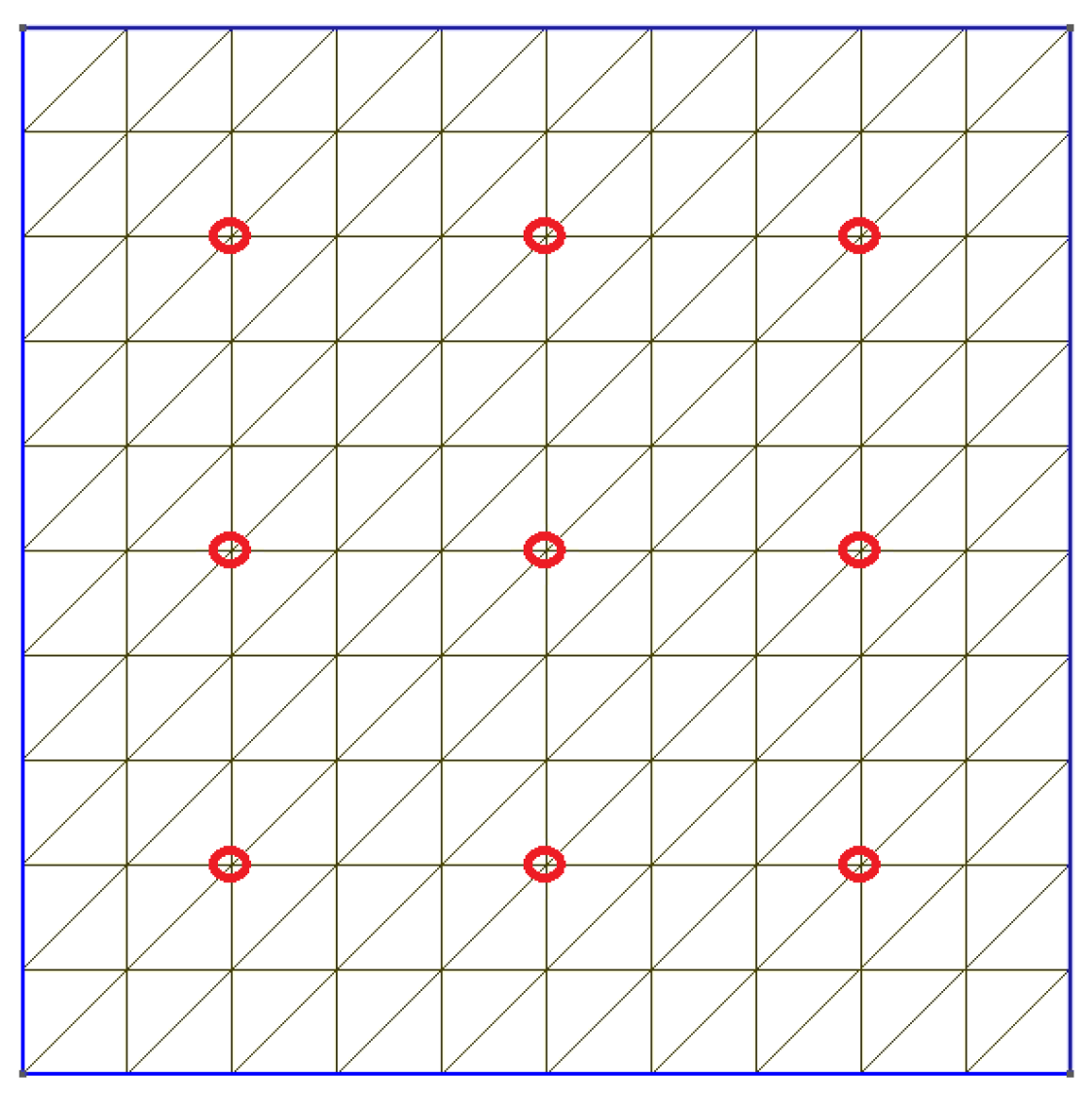
Figure 1 presents an example of selected interpolation nodes. We will use this interpolation method for our machine learning approach presented in the next section.

5. Machine Learning Approach

Training neural networks to solve the poroelasticity problem is complex and time-consuming. As a result, it makes more sense to make training the computationally expensive part of the solution—the implicit flow part. Due to the inefficiency of training all degrees of freedom, we propose training only a portion of the solution. We train the neural network to obtain the high-conductive continuum’s pressure at multiple mesh nodes at some time steps. Then, we apply the DEIM spatial interpolation and linear time interpolation. As a result, we treat the high-conductive continuum’s pressure as a known function that we may use to find the other pressure.

A basic DNN is made up of layers, each of which uses a differentiable function to translate one volume of activations to another. The layers of a neuron network are nonlinear transformations. The previous layer’s output result is transmitted to the following layer. The neurons of the previous layer are linked to the neurons of the current layer, and the connection data are a weighting parameter. As a result, the neural network training aims to perfect the weights. Deep neural networks use a nonlinear operation to minimize the amount of input data and simplify the task. We use TensorFlow’s most straightforward DNN variation in the sequential model [26]. The generation of the dataset used to train is essential in machine learning. The final need is to create an appropriate neural network architecture.

A neural network function $\mathcal{N}$ of L—layers with samples x—input data and y—output data may be represented in the following form in deep learning.

$${\mathcal{N}}^L(x,\theta )={\sigma }^L(W^L{\sigma }^{L-1}(\cdots {\sigma }^2(W^2{\sigma }^1(W^{1}x+b^1)+b^2)\cdots )+b^L),$$

where Ws are weight matrices, bs are bias vector, and $\sigma$s are the activation functions, where $\sigma ->\mathrm{RELU}=max(0,x)$.

Let us write:

• The first output layer: ${\mathcal{N}}^1\left(x^0\right)=Y^1$, i.e., $Y^1={\sigma }^1(W^{1}x+b^1)$;
• For i’s layer: $Y^i={\sigma }^i(W^i{x}^{i-1}+b^i)$, where i = 1,2,…, L.

For estimating the output y, a neural network called ${\mathcal{N}}^L$ is employed. The goal of the neural network is to solve an optimization problem to identify parameters ${\theta }^{*}$.

$${\theta }^{*}={\mathrm{argmin}}_{\theta }\frac{1}{N}\sum _{j=1}^N\left|\right|y_j-\mathcal{N}(x_j;\theta ){\left|\right|}_2^2,$$

where N is the number of the samples. Here, $\frac{1}{N}{\sum }_{j=1}^N\left|\right|y_j-\mathcal{N}(x_j;\theta ){\left|\right|}_2^2$ is the loss function—$L\left(\theta \right)$.

We generate a network ${\mathcal{N}}^L(x,\theta )$ using:

• Activation function: ReLU (Rectified Linear Unit) activation function for all layers (first input and hidden layers), no activation function at the last output layer;
• DNN structure: 2 hidden layers, each layer comprises 12 neurons;
• Kernel initializer: normal for input and output layers and he_normal for all hidden layers;
• Training optimizer: Adam.

We chose the activation function ReLU because it has shown effectiveness in deep neural network training without experiencing a vanishing gradient problem.

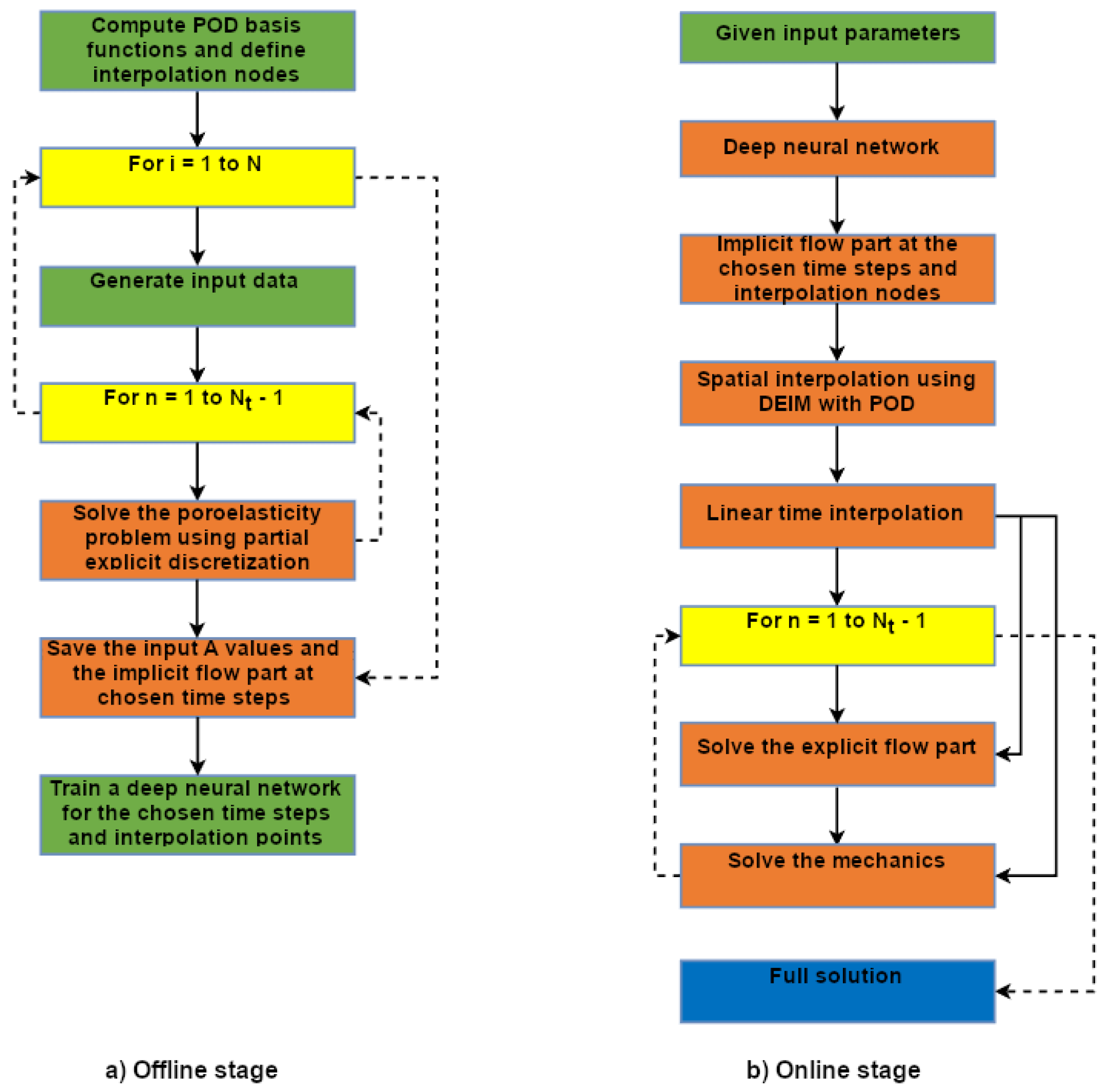
Therefore, our method consists of two stages: offline and online. In the offline stage, we compute the POD basis functions and interpolation nodes, generate (or receive) data, and train the neural network to obtain high-conductive continuum pressure in the interpolation nodes. In the online stage, we can already solve the problem for an arbitrary set of input parameters. We pass the input data to the neural network, which gives the pressure values at the interpolation nodes. We perform spatial and temporal interpolation and solve the problem by treating the pressure of the high-permeability continuum as a known function. Figure 2 depicts a block diagram of our method’s offline and online stages.

6. Numerical Results

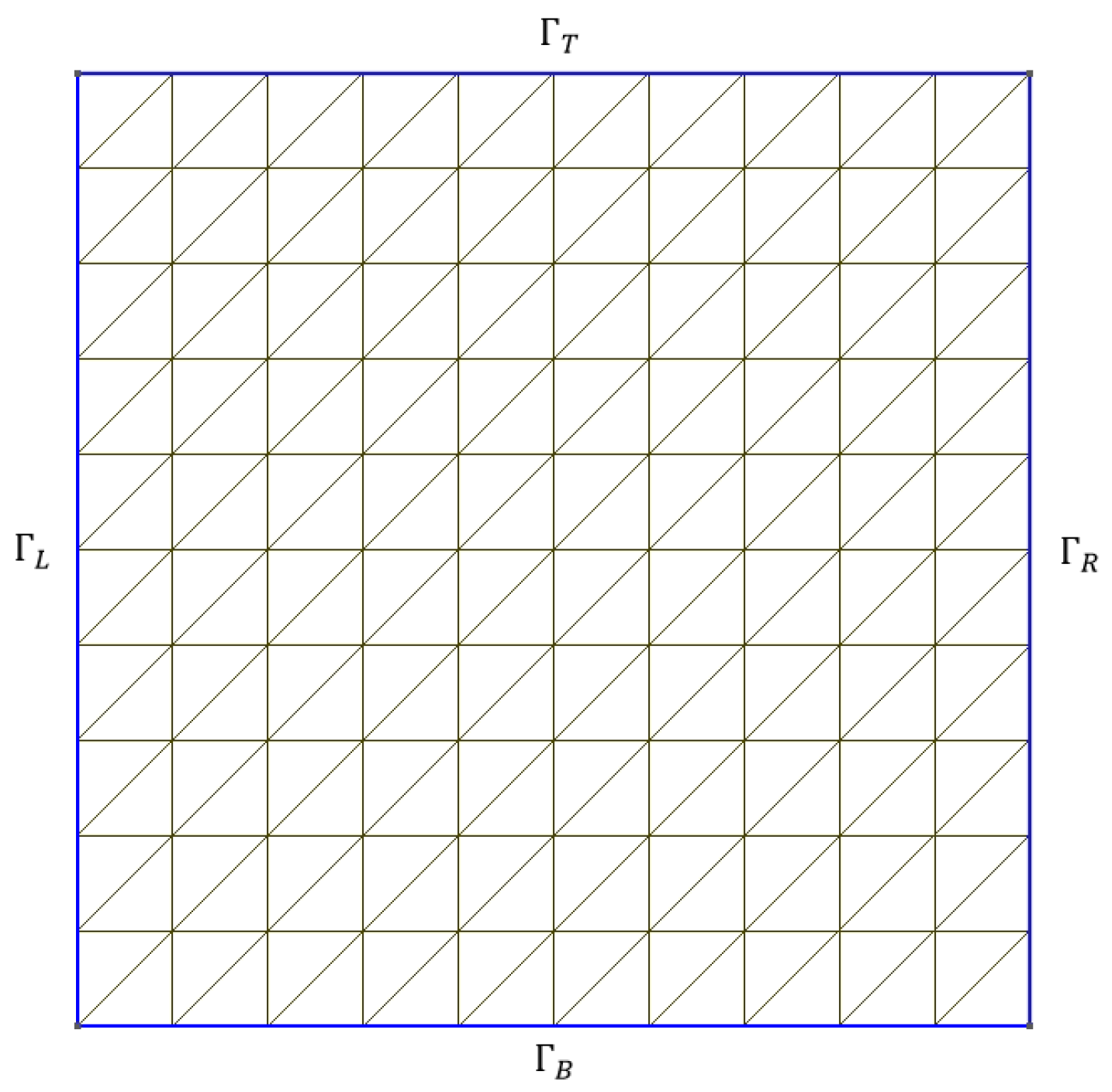
This section considers the numerical solution of the poroelasticity problems in dual continuum heterogeneous media. As a computational domain, we consider $\Omega =[0,1]\times [0,1]$. We use a structured computational mesh with 121 vertices and 200 cells (see Figure 3). For model problem parameters, we set $M_1=M_2=1$, ${\alpha }_1={\alpha }_2=1.0,\nu =0.3$. The calculation is performed by $T_{max}=1$ with time step $\tau =0.01$. For the initial conditions, we set $p_0=0$ and $u_0=0$. 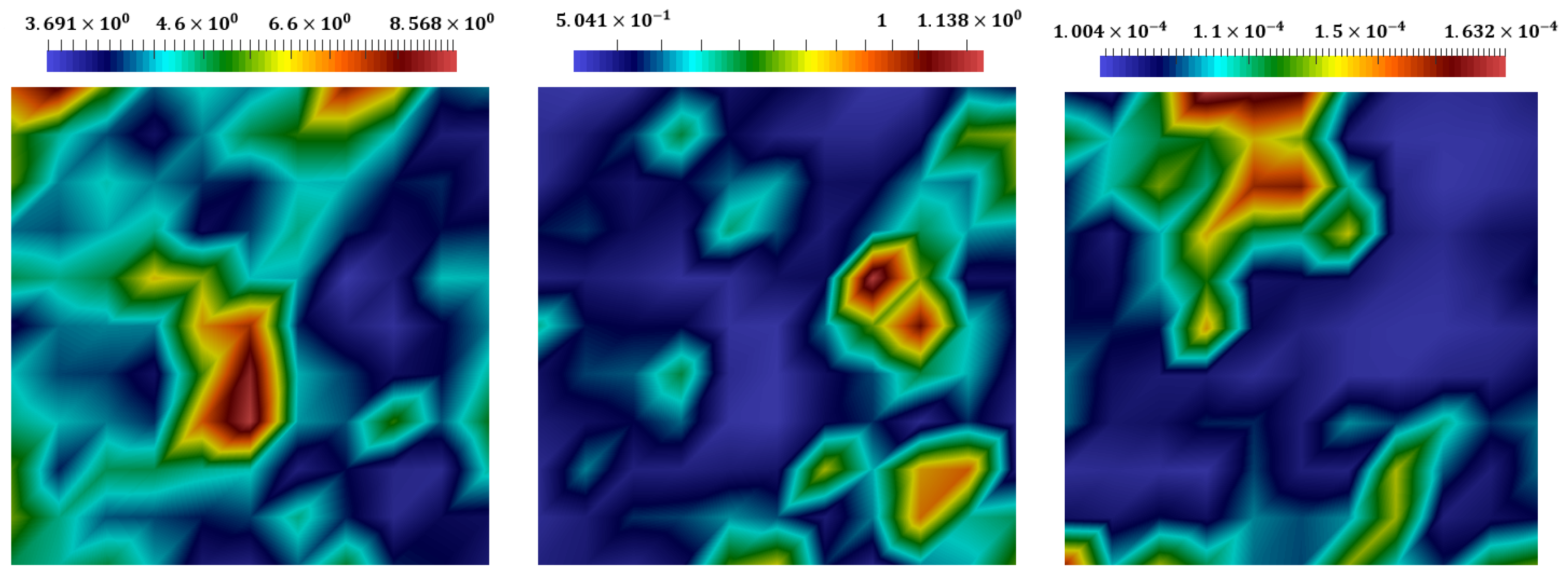The eterogeneous coefficients for elasticity modulus E and heterogeneous permeability k for the first and second continua are presented in Figure 4. We set the parametric function $g={\sum }_{i=1}^{N_a}{A}_{i}sin\left(i\pi x\right)sin\left(i\pi y\right)sin\left(it\right)$, where $N_a=5$, and the value range $A_i\in [-1,1].$

Note that this paper focuses mainly on developing a solution method, so we consider only the two-dimensional case. However, our approach can be beneficial for more complex problems, such as modeling three-phase and three-dimensional materials. Solving such problems will not require any significant changes to the algorithm.

GMSH software was used to construct the computational domains and meshes [27]. The numerical realization of the problem was based on finite element approximation using the FEniCS computing platform [28]. For partial learning implementation, we used Keras [29]—a high-level API for the TensorFlow machine learning platform [26]. Finally, visualization of the numerical results was based on the ParaView software [30].

Our neural network aimed to find the high-conductive continuum pressure at nine interpolation points. As mentioned before, we used the Discrete Empirical Interpolation Method (DEIM) to perform the spatial interpolation. The first step of the DEIM was generating snapshot functions. To generate them, we solved the problem five times with different values of $A_i$. We saved the results every second time step. Therefore, we obtained $N=250$ snapshots. Then, we solved a spectral problem and obtained nine basis functions. Using the DEIM algorithm, we selected nine optimal interpolation nodes. Next, we trained the neural network to obtain the high-conductive continuum pressure at these interpolation points.

The neural network considered random $A_i$ values as the input and the high-conductive continuum pressure at nine interpolation points as output. Thus, the input data size was five, and the output data size was nine. We solved the problem 300 times with randomly generated $A_i$ values to prepare a training dataset. For a test dataset, we solved the problem 20 times with $A_i$ that were absent from the training dataset. Then, we performed spatial and time interpolations.

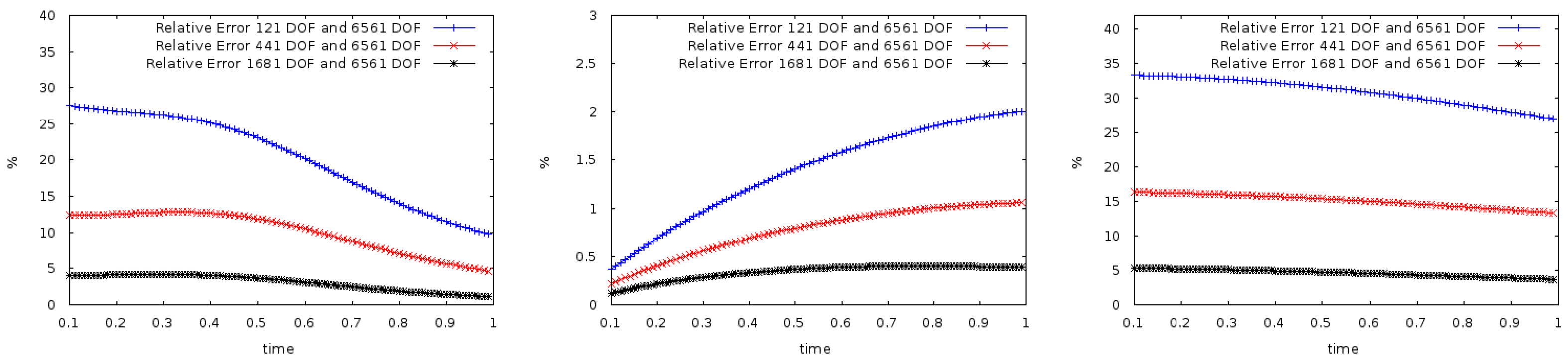
We used relative errors $L_2$ between the reference solution and the proposed approach’s solution to compare the results. We performed multiple tests to determine the errors caused by different steps of our approach.

$$e_{L^2}^{p_1}={\left(\frac{{\int }_{\Omega }{(p_1^{ref}-p_1^{appr})}^{2}dx}{{\int }_{\Omega }{\left(p_1^{ref}\right)}^{2}dx}\right)}^{1/2}·100\%,e_{L^2}^{p_2}={\left(\frac{{\int }_{\Omega }{(p_2^{ref}-p_2^{appr})}^{2}dx}{{\int }_{\Omega }{\left(p_2^{ref}\right)}^{2}dx}\right)}^{1/2}·100\%,$$

$$e_{L^2}^u={\left(\frac{{\int }_{\Omega }{(u^{ref}-u^{appr})}^{2}dx}{{\int }_{\Omega }{\left(u^{ref}\right)}^{2}dx}\right)}^{1/2}·100\%,$$

where the superscript $ref$ denotes the reference solution, and the superscript $appr$ denotes the approximate solution. We considered different methods depending on the part of the error we wanted to evaluate.

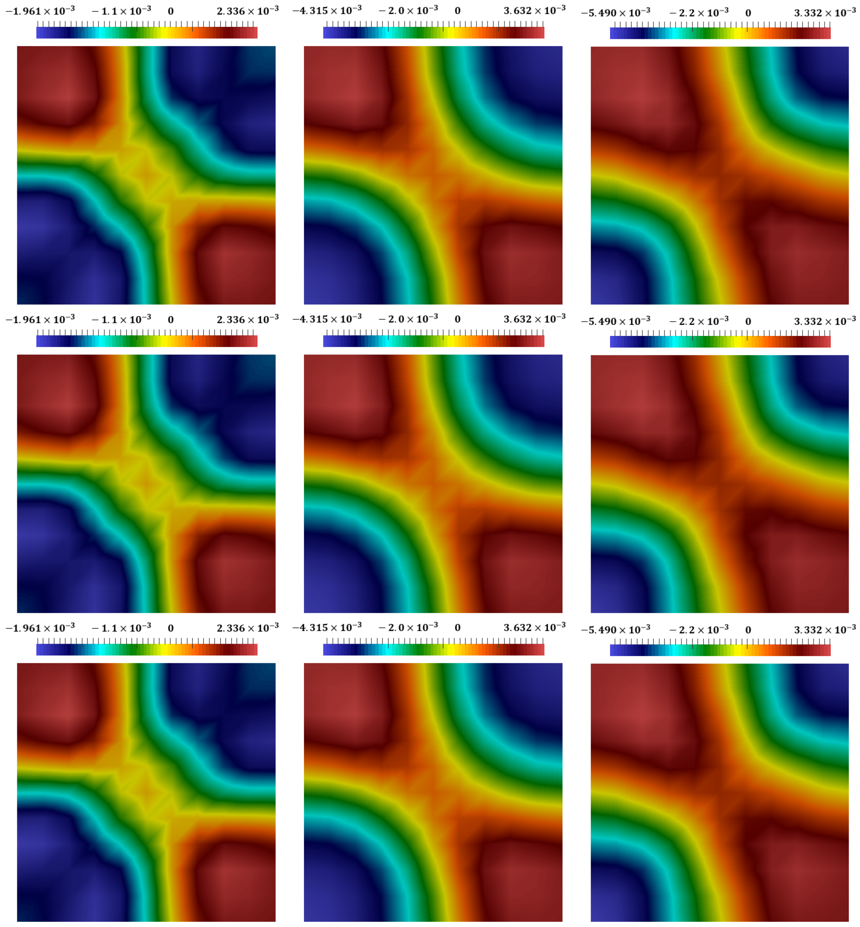
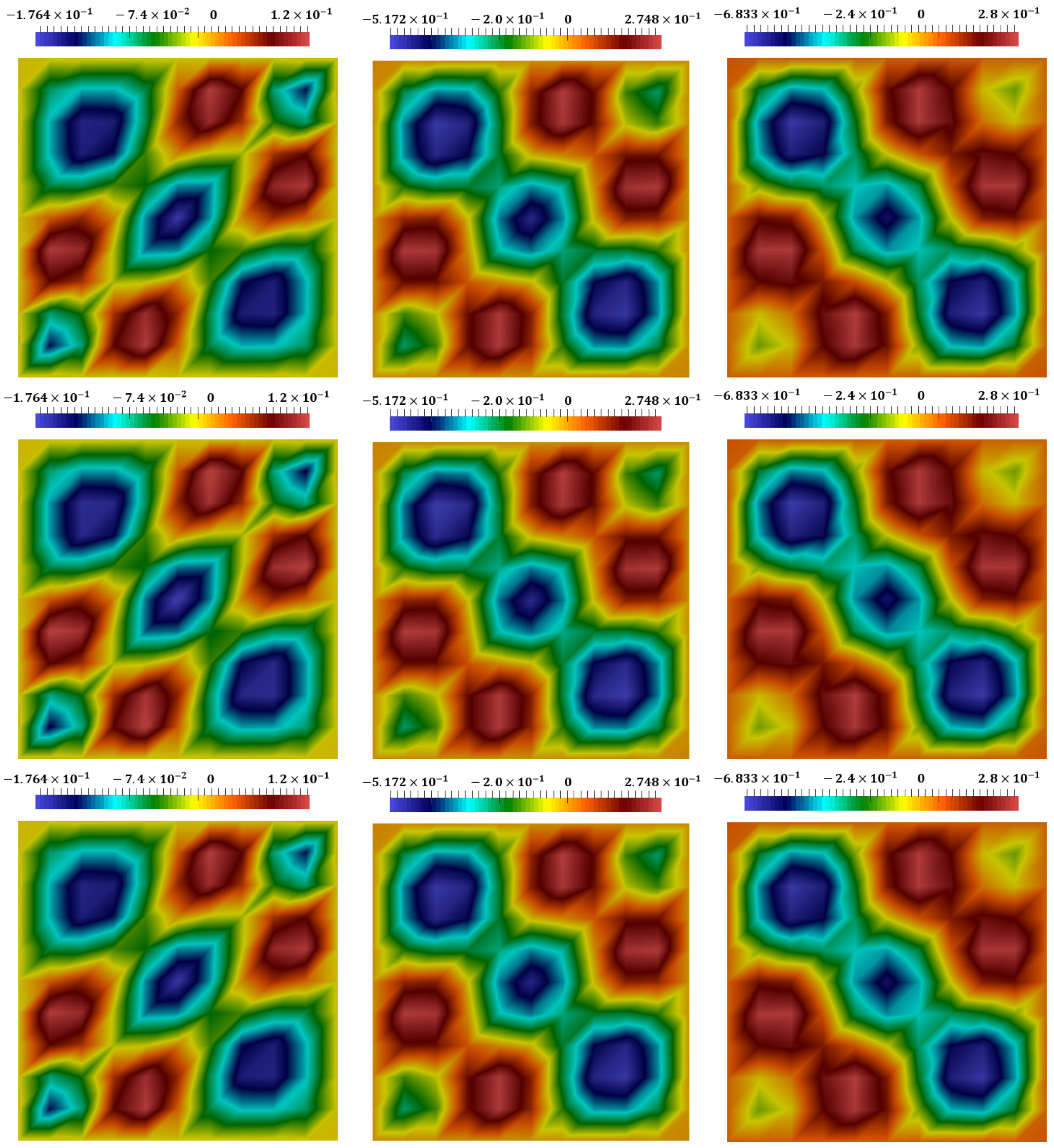
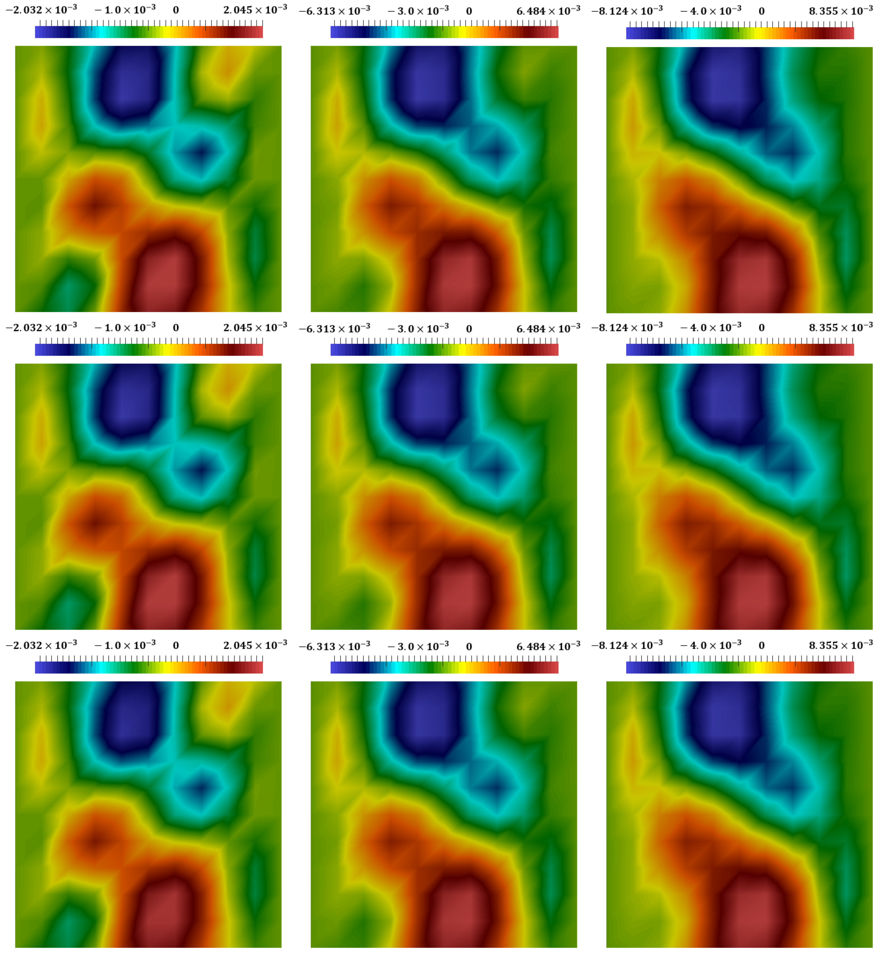
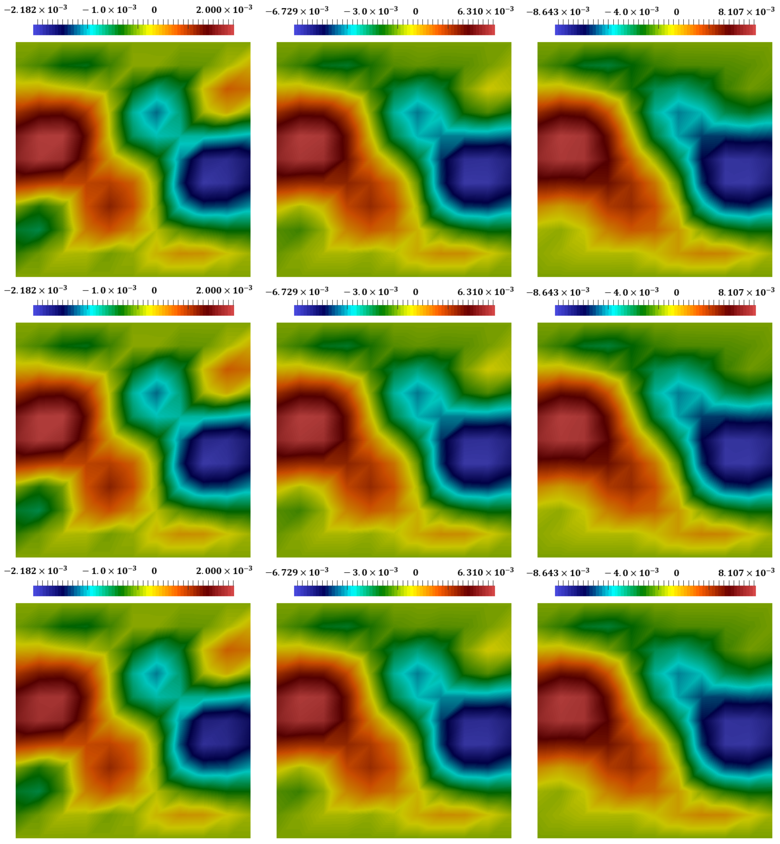
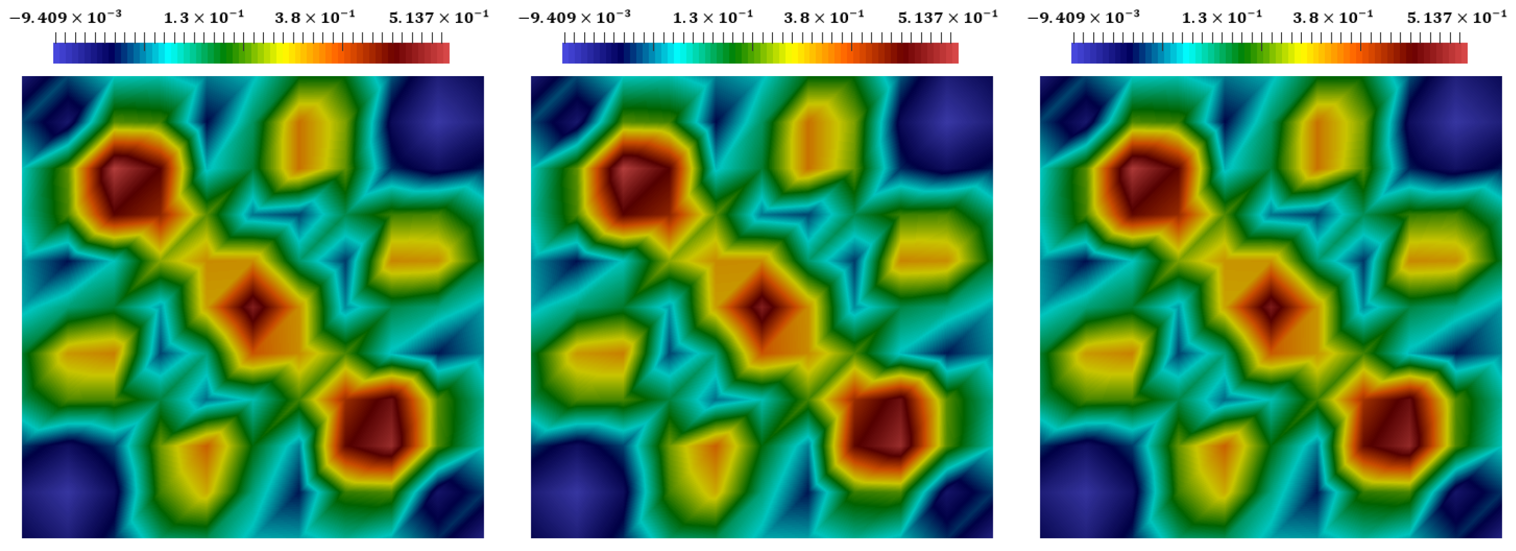
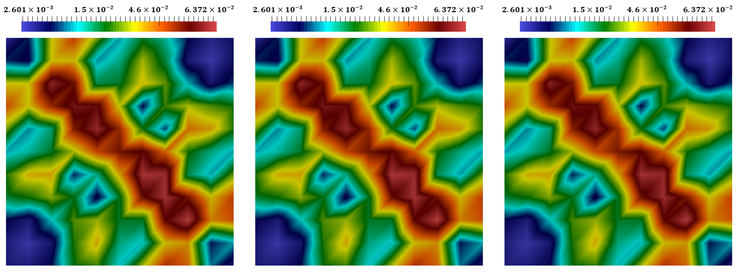
Figure 5, Figure 6, Figure 7 and Figure 8 present the distributions of pressures for the first and second continua and the displacements in $x_1$ and $x_2$ directions at different time steps ($t_m$ with $m=0.4,0.8,1$). In each figure, we depicted the solutions using the coupled explicit–implicit scheme, the split explicit–implicit scheme, and the proposed approach (from top to bottom). Because all results were very similar, we can conclude that our proposed method can provide good accuracy.

In Figure 9, we studied the dependence of accuracy on the computational mesh. As a reference mesh, we took the finest mesh (6561 vertices) and compared its results with the results of coarser meshes (121, 441, and 1681 vertices) for the first and second continuum and displacement. Figure 10 and Figure 11 describe the distributions of strain and stress at the final time.

7. Conclusions

This work considered the poroelasticity problem in dual continuum heterogeneous media. For the mathematical model, we used dual continuum flow and the effective stress that contained terms of both continua. We applied a finite element method with standard linear basis functions for the spatial approximation. Furthermore, we used the explicit–implicit scheme for the time approximation, where the explicit scheme was used for the low-conductive continuum, and the implicit scheme was applied for the high-conductive one.

We proposed a new method based on hybrid explicit–implicit (HEI) learning to solve the poroelasticity problem in dual continuum heterogeneous media. The method’s main idea was to train a Deep Neural Network to predict the implicit flow part at some node at some time steps. Then, we performed the DEIM interpolation and linear time interpolation. After that, we treated the high-conductive continuum’s pressure as a known function and solved the whole problem. We considered the two-dimensional model problem to test the proposed method. We solved the problem using various methods to evaluate errors in the different steps of our method. The results demonstrated that the proposed approach can successfully solve the poroelasticity problems in dual continuum heterogeneous media.