New Applied Problems in the Theory of Acyclic Digraphs

Abstract

The following two optimization problems on acyclic digraph analysis are solved. The first of them consists of determining the minimum (in terms of volume) set of arcs, the removal of which from an acyclic digraph breaks all paths passing through a subset of its vertices. The second problem is to determine the smallest set of arcs, the introduction of which into an acyclic digraph turns it into a strongly connected one. The first problem was solved by reduction to the problem of the maximum flow and the minimum section. The second challenge was solved by calculating the minimum number of input arcs and determining the smallest set of input arcs in terms of the minimum arc coverage of an acyclic digraph. The solution of these problems extends to an arbitrary digraph by isolating the components of cyclic equivalence in it and the arcs between them.

1. Introduction

The monographs [1,2,3], which have become classic, are devoted to theoretical and applied issues of digraph research. They are closely related to the Ford–Fulkerson theorem on the equality of the maximum flow and the minimum cut [4,5]. At first glance, many problems with digraphs look like NP-problems. However, with a special selection of optimized indicators and graph transformation, these tasks can be reduced to the search for Ford–Fulkerson algorithms. In this way, it becomes possible to avoid the appearance of NP-problems when working with digraphs. Therefore, these studies can be attributed to the intensively developing applications of digraph theory in system analysis and the theory of optimization algorithms on graphs [6,7]. The papers closest to the subject of this article can be considered [8,9].

In particular, the strong connectivity in digraphs is considered in the presence of arc failures [10]. The paper [11] studies the use of digraphs in interferometry. The paper [12] explores the issues of spectral complexity of digraphs and their application to structural decomposition. In [13], using digraph models, the issues of signal processing and learning from network data are analysed. In the work [14], the multilevel task of identifying bottlenecks in the network is considered. In the works [15,16], minimal networks are built in which the Ford–Fulkerson procedure may not be completed. The paper [17] explores various ways of applying stochastic models on digraphs in computational biology. Due to the intensive development of biotechnology, two new applied problems of digraph theory are posed in this paper, which require both the development of the theory and the construction of new optimization algorithms on digraphs. Both tasks were initiated by biotechnological problems related to protein networks. Let us describe these tasks in more detail.

The importance of analysing protein networks in plant bioengineering is due to the fact that the growth and development of plants, as well as their protective functions, are regulated by the interaction of various protein signalling modules. At the same time, fine-tuning of metabolic processes takes place, allowing the plant to adapt to changing environmental conditions. Plant interactomes have not been worked out enough yet. Therefore, it is necessary to develop mathematical modelling methods that describe the natural functions of protein modules as accurately as possible.

Previously, we tried to link various cellular processes affecting the biosynthesis of anthocyanins. In this work, we have identified the main signalling protein modules that regulate the biosynthesis of anthocyanins. As far as we know, this was the first reconstruction of a network of proteins involved in the secondary metabolism of plants [18].

It was further shown that the signalling systems of abscisic acid (ABA) and chaperones are integrated by chromatin remodelling proteins (CRC) into a single regulatory network. CRC proteins “remember” the previous stressful effects and adjust the plant to the perception of new ones, and memory is generated in the offspring. A new scientific direction—“bioengineering of memory” was substantiated [19].

Fabregas et al. [20] reported that overexpression of the vascular brassinosteroid receptor BRL 3 provides improved drought resistance without disrupting plant growth. We have constructed a network of protein–protein interactions of ABA and brassinosteroid signalling systems. It has been established that the phenomenon of drought resistance mediated by BRL3 can be explained by the generation of stress memory (a process known as “priming” or “acclimation”) [21]. Let us now turn to the mathematical formulation and algorithmic solution of the protein network modelling.

In the first problem, we are talking about finding a smallest set of arcs, the removal of which blocks all paths passing through an acyclic digraph with a set of W (corrupted) vertices. To solve this problem, it is proposed to cut the pathways entering the set of affected proteins or leaving this set, thus minimizing the number of cut paths. Such minimization deforms the structure of the protein network in the least way. It should be noted that isolation measures restricting the normal functioning of various communication networks, such as transport, economic, educational, etc., have recently invaded our lives. Therefore, the considered biotechnological problem acquires a more general meaning, which requires the construction of economical algorithms for its solution.

In biotechnology there is a problem to decrease a number of blocking arcs. To solve this problem it is possible to add to incoming and out coming arcs some arcs between corrupted vertices (selected by the biotechnologists) and to choose among them minimal number of blocking arcs. This procedure may be realized by implementing a large bandwidth to chosen arcs. All its stages are well known, but together they make it possible to solve an important and new problem in the field of biotechnology. Thus, it becomes possible to structure both the formulation and the solution of this problem, taking into account the choice of biotechnologists.

The solution of this problem is based on a special building of the integer bandwidths of the arcs of an acyclic digraph, the minimum section in which contains only of arcs entering from the inside into the subset W and/or exiting from the inside of the subset W and some arcs between vertices from W. By choosing the integer bandwidths, the arcs connecting the vertices of the subset $U_{*}$, are made unsaturated by the maximum flow. In turn, saturated with the maximum flow (the maximum flow passing through them coincides with their throughput) can only be arcs entering from the outside into a subset of W and/or exiting from the outside of the subset W. Next, the minimal section is searched using the well-known Ford–Fulkerson algorithm [4,5], which guaranteed to converge only for integer throughput. This algorithm was developed in its modifications [22,23]. Minimizing the number of arcs satisfying certain properties creates a risk of encountering an NP-problem as the problem of continuous brute force. The use of techniques that lead the tasks to the modified Ford–Fulkerson algorithm allows us to avoid the risk of NP-complex problems. Thus, in order to use the Ford–Fulkerson algorithm in solving this problem, it is necessary to build a two-pole and select the integer throughputs of its arcs so that the solution obtained in this algorithm determines the solution of the problem.

An alternative and in some sense inverse second problem is connected with the introduction into the digraph of a smallest set of new arcs that turn an acyclic digraph into a strongly connected one (in which there is a path from any vertex to any other vertex). This procedure is needed to include all the vertices of the acyclic digraph in the feedbacks that stabilize the functioning of the network represented by the digraph.

To do this, we first consider a bipartite acyclic digraph, in which all arcs are directed from the first lobe to the second. By removing the orientation of the arcs, we obtain an undirected bipartite graph. Using the well-known generalizations of the Ford–Fulkerson [24] algorithm, the maximum matching is searched for in it by a method of increasing alternating paths [25], from which the minimum arc cover is constructed. It consists of an incoherent collection of star-like sub graphs (in which arcs connect some vertices with the base of the star) ([26] p. 318). Next, the orientation of the arcs is restored and additional arcs are introduced in the resulting bipartite digraph by a special algorithm. This algorithm is based on the sequential arrangement first of the stars of the first type-with roots in the first lobe and then of the stars of the second type with roots in the second lobe. If all the stars have the same type, then their vertices may be connected by a Hamiltonian cycle [27].

However, if there are stars of different types, then the stars of the first and then the second type are located first. Then, additional arcs are introduced from the vertices of the second lobe to the vertices of the first lobe so that their number equals the maximum between the number of vertices of the first lobe and the second lobe. This number of additional arcs is minimal for obtaining strongly connected digraph. When moving from the minimum arc cover to the original bipartite digraph, the minimum number of additional arcs cannot increase. At the same time, the set of additional arcs already found transforms this bipartite digraph into a strongly connected one. The transition from an arbitrary acyclic digraph to a bipartite one is based on the allocation in an arbitrary digraph of the first lobe, including vertices from which only arcs come out, and the second lobe, including vertices that only arcs enter. An arc between the vertex of the first lobe to the vertex of the second lobe in a bipartite digraph is drawn if and only if there is a path between these vertices in the original digraph.

When solving both problems, we have to deal with digraphs that are not initially acyclic. The transformation of an arbitrary digraph into an acyclic one is based on the procedure for allocating cyclic equivalence classes (in which there is a path from any vertex to any other vertex) and arcs between them [28]. The paper presents an original algorithm for solving the problem of allocating cyclic equivalence classes [29] basing on the sequential inclusion in the digraph of a new vertex and arcs connecting it to the already specified ones.

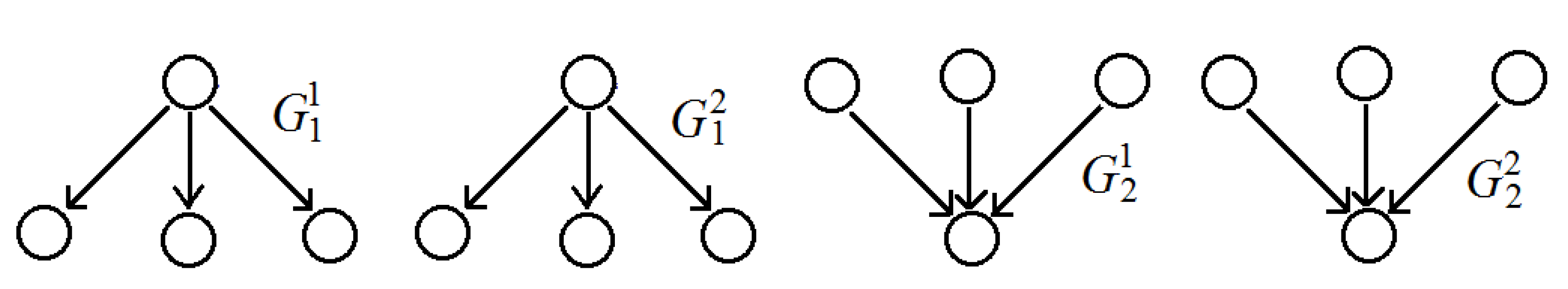
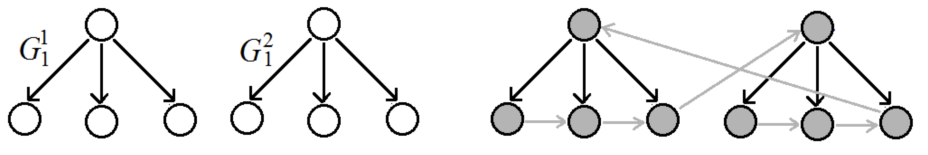
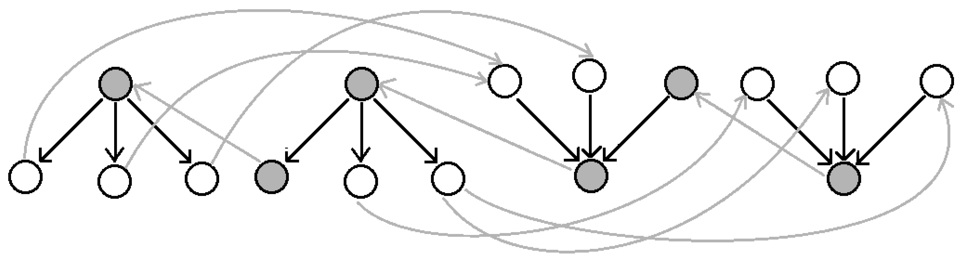
2. Optimal Blocking of Selected Vertices of the Acyclic Digraph

Consider an acyclic digraph $\mathcal{G}$, with a finite set of vertices $\mathcal{U}$ and a finite set of arcs $\mathcal{V}$. In the set $\mathcal{U}$, a subset $U\subset \mathcal{U}$ of the so-called corrupted vertices is allocated. Let’s define an acyclic digraph $G\subset \mathcal{G}$, with a set of vertices U and a set of arcs V connecting these vertices.

We attach to the digraph G the arcs of the digraph $\mathcal{G}$, walking to the set U from the set $\mathcal{U}\backslash U$ and the arcs coming out of U to $\mathcal{U}\backslash U$ and some arcs from the set $\mathcal{U}$, selected by biotechnologists. The set of these arcs is denoted by W and we call the path passing through the set U in the digraph $\mathcal{G}$, if it starts at the vertex of the set $\mathcal{U}\backslash U$ moves by an arc of W to the set U, passes through the set U and then moves by an arc of the set W to the set $\mathcal{U}\backslash U$. Our task is to determine in the set W the smallest subset of arcs whose removal from the digraph $\mathcal{G}$ breaks all paths, passing through the set of vertices U.

To do this, we transform the digraph G together with the set of its incoming and out coming arcs into the digraph $G^{\prime }$ as follows. All vertices of the set $\mathcal{U}\backslash U$, from which arcs of the set W move to U we combine into one vertex S and call it the source. All vertices of the set $\mathcal{U}\backslash U$, to which arcs of the set W move from U we combine into one vertex T and call it a drain. All arcs of the set W, going from the source S to the vertex $P\in U$, we combined into one arc $w_{*}$ and determine its throughput equal to $n\left(P\right)$, which is the number of arcs to be combined. All arcs of the set W, going from the vertex $P\in U$ to the drain T, we combine into one arc $w^{*}$ and determine its throughput equal to $N\left(P\right)$. If there is not an arc from the source S to vertex P, then $n\left(P\right)=0$, if there is not an arc from the vertex P to the drain T, then $N\left(P\right)=0$ as well.

Note that to formulate the optimization problem, it is necessary to exclude from its solution all arcs of the set V, which are not chosen by biotechnologists. To realize this procedure denote ${\displaystyle L=min\left(\sum _{P\in U}n\left(P\right),\sum _{P\in U}N\left(P\right)\right)}$ and assign the bandwidth $L+1$ to all arcs of the digraph $G^{\prime }$, which are not included in the set W. All arcs of the digraph $G^{\prime }$, which are chosen by biotechnologists, receive bandwidth 1. Therefore, the acyclic digraph $G^{\prime }$ becomes the bipolar, that is the digraph with the single vertex S, which has only out coming arcs, and the single vertex T, which has only incoming arcs.

Proposition 1.

The quantity of maximal flow in the bipolar $G^{\prime }$ is not larger than L.

Proof of Proposition 1.

Indeed, the quantity of maximal flow in the bipolar $G^{\prime }$ is not larger than a sum ${\displaystyle \sum _{P\in U}n\left(P\right)}$ of weights of arcs moving from the source S. The quantity of maximal flow in the bipolar $G^{\prime }$ is not larger than a sum ${\displaystyle \sum _{P\in U}N\left(P\right)}$ of weights of arcs moving from the drain T. Consequently, the quantity of the maximal flow in the bipolar $G^{\prime }$ is not larger than ${\displaystyle L=min\left(\sum _{P\in U}n\left(P\right),\sum _{P\in U}N\left(P\right)\right)}$. □

Proposition 2.

If in bipolar $G^{\prime }$, some arc w has bandwidth $L+1$, then it does not include into any minimal cut.

Proof of Proposition 2.

From the theorem of Ford–Falkerson [4,5], it is clear that any minimal cut in the bipolar $G^{\prime }$ consists only of arcs saturated by any maximal flow. Therefore, the arcs which have bandwidths $L+1$ cannot be included into any minimal cut. □

Remark 1.

It follows from Propositions 1 and 2 that the proposed method for setting the bandwidths in the two-pole $G^{\prime }$ allows determining the minimum cuts only from the arcs of the set W, as required in the original formulation of the problem.

As all included bandwidths are integers, using the Ford–Fulkerson algorithm [4,5] (or its modifications [22,23]) it is possible to calculate the maximum flow in the digraph $G^{\prime }$ and to obtain minimal cut $W^{\prime }$. Each of the arcs of the set $W^{\prime }$, going from S to $P\in U$ is defined as the union of $n\left(P\right)$ arcs of the digraph $\mathcal{G}$. Similarly, each of the arcs of the set $W^{\prime }$, going from $P\in U$ to T is defined as the union of $N\left(P\right)$ arcs of the digraph $\mathcal{G}$. Denote $W^{″}$ a set of arcs from the set W, included in the combined arcs of the set $W^{\prime }$. Consequently from Propositions 1 and 2 and Remark 1 we have that $W^{″}$ is the solution of the optimization problem of selecting a smallest set of arcs from the set W whose removal breaks all paths passing through the vertex set of U. Indeed, if the united arc $w\in W^{\prime }$, then to block all paths passing through the vertex set U, we must delete all arcs, united in an arc w.

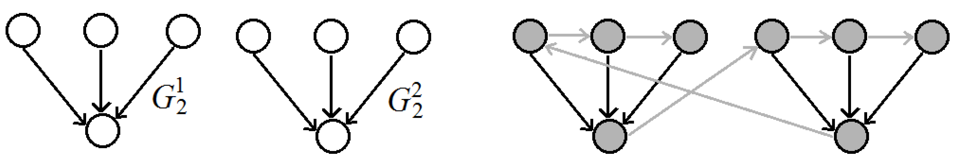
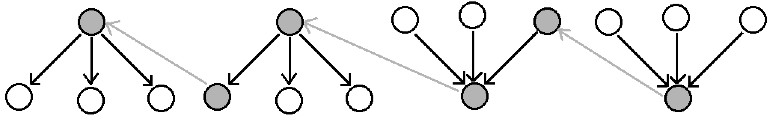
3. Optimal Algorithm for Converting an Acyclic Digraph into a Strongly Connected One

Problem statement. Suppose that a complex system, for example, a protein network, is represented by an acyclic digraph $\mathcal{G}$ without loops and isolated vertices. Let’s denote $V_1$ the set of vertices from which the arcs only come out, and $V_2$ the set of vertices into which the arcs only enter. Now let’s construct a bipartite digraph G, in which the set of vertices of the first lobe $V_1$, and the set of vertices of the second lobe $V_2$, the vertex $v_1\in V_1$ is connected to the vertex $v_2\in V_2$ by an arc, if there is a path between them in the acyclic digraph $\mathcal{G}$. As the digraph $\mathcal{G}$ is acyclic so there are not ways from vertices of the second lobe $V_2$ to vertices of the first lobe $V_1$. We denote $p\left(\mathcal{G}\right)$ the smallest set (by a number of arcs) of additional arcs (call them “good arcs”), the introduction of which in $\mathcal{G}$ transforms it into a strongly connected digraph and designate $\left|p\right(\mathcal{G}\left)\right|$ the number of good arcs in $p\left(\mathcal{G}\right)$.

Let us transform a bipartite digraph G into an undirected one by removing the orientation of the arcs and find a minimal arc cover in it (see, for example, [6,24]). To do this, using the algorithm of increasing alternating paths, we find the maximum matching that can be transformed into a minimum arc cover, whose connected components are star-like sub graphs (all arcs come from one vertex or enter one vertex, called the root). In the minimal arc cover, we restore the direction of the arcs and denote the resulting bipartite digraph $\widehat{G}$. It should also be noted that there are two types of star-like sub graphs. In the star-likesub graph of the first type, the root is contained in the first lobe $V_1$ (on the left in Figure 1) and in the star-like sub graph of the second type, the root is contained in the second lobe $V_2$ (on the right in Figure 1).

The main result of the work is an algorithm for constructing a smallest set of good arcs that turn $\widehat{G}$ into a strongly connected digraph. It is proved that the number of good arcs in a smallest set $p(\widehat{G})=max\left(\right|V_1|,|V_2\left|\right)$, where $|V_i|$ the number of vertices in the set $V_i,i=1,2$. This equation applies to a bipartite graph G with lobes $V_1,V_2$ and to acyclic digraph $\mathcal{G}$. This is due to the fact that “good arcs,” turning the bipartite digraph $\widehat{G}$ into strongly connected, also turn the bipartite digraph G and the original acyclic digraph $\mathcal{G}$ into strongly connected.

Main results. Consider a bipartite digraph $\widehat{G}$, consisting of the set of unrelated M stars $G_1^1,\dots ,G_1^M$ with the root in the first lobe and N stars $G_2^1,\dots ,G_2^N$ with the root in the second lobe. Let m the number of leaves in the stars $G_1^1,\dots ,G_1^M$ and n the number of leaves in the stars $G_2^1,\dots ,G_2^N$. Then, it performs equality $|V_1|=M+n,|V_2|=m+N$. Figure 1 shows an example of a digraph $\widehat{G}$, consisting of stars $G_1^1,G_1^2,G_2^1,G_2^2$ in the case of $m=n=6,M=N=2$. Here, the upper vertices make up the first lobe, and the lower ones make up the second lobe.

Theorem 1.

Equality $|p(\widehat{G})|=max(|V_1|,|V_2\left|\right)$ is true.

Proof of Theorem 1.

When converting the digraph $\widehat{G}$, the number of good arcs, entering the roots of stars $G_1^1,\dots ,G_1^M$, must be no less than M, and entering the leaves of stars $G_2^1,\dots ,G_2^N$—no less than n. The number of good arcs, leaving the leaves of stars $G_1^1,\dots ,G_1^M$, must be no less than m, and leaving the roots of the stars $G_2^1,\dots ,G_2^N$ are no less than N. Therefore, the number of good arcs entering the vertices of the first lobe is no less than $M+n$, and leaving the vertices of the second lobe is no less than $m+N$. Additional incoming and outgoing arcs may coincide. Therefore, the minimum number of additional arcs is $|p(\widehat{G})|\ge max(m+N,n+M)$. Now, we prove that $|p(\widehat{G})|=max(M+n,m+N)=max\left(\right|V_1|,|V_2\left|\right)$.

Let us first consider the case when the digraph $\widehat{G}$ consists only of stars $G_1^1,\dots ,G_1^M$ or only of stars $G_2^1,\dots ,G_2^N$. Let us add stars $G_1^1,\dots ,G_1^M$ by good arcs.

In the stars $G_1^1,\dots ,G_1^M$ with good arcs, we indicate the Hamiltonian cycle. It starts at the root of the star $G_1^1$, passes sequentially through all the leaves of this star, goes to the root of the star $G_1^2$, etc., from the last leaf of the star $G_1^M$ to the root of the star $G_1^1$. As a result, we transform the stars $G_1^1,\dots ,G_1^M$ into a strongly connected digraph with the number of additional arcs $m=max(m+0,0+M)$ (Figure 2). If $M=1$, then the last leaf of the star $G_1^1$ is connected by the good arc with its root.

Similarly, in the digraph $\widehat{G}$, consisting only of stars $G_2^1,\dots ,G_2^N$, let us add these stars with good arcs sequentially connected by their leaves. In addition, from the root of the star $G_2^k$, we will draw a good arc to the first leaf of the star $G_2^{k+1},k=1,\dots ,N-1$, and from the root of the star $G_2^N$ to the first leaf of the star $G_2^1$. If $N=1$, we connect the root of the star $G_2^1$ with its first leaf.

In the stars $G_2^1,\dots ,G_2^N$ with additional arcs, we indicate the Hamiltonian cycle. It starts in the first leaf of the star $G_2^1$, passes sequentially through all its leaves, and goes to its root, then goes to the first leaf of the star $G_2^2$, etc. From the root of the star $G_2^N$, the path continues to the first leaf of the star $G_2^1$. As a result, we transform the stars $G_2^1,\dots ,G_2^N$ into a strongly connected digraph with the number of additional arcs $n=max(0+N,n+0)$ (Figure 3). If $N=1$, we connect the root of the star $G_2^1$ by the good arc with its first leaf.

Let us now consider the case when $MN>0$, i.e., in the digraph $\widehat{G}$, there are stars of both the first and the second types. Denote $W_1$ the set of all vertices in the stars $G_1^1,\dots ,G_1^M$ and $W_2$ the set of all vertices in the stars $G_2^1,\dots ,G_2^N$. Let us introduce a good arc, coming out of the root of the star $G_2^N$ and entering some leaf of the star $G_2^{N-1}$, an arc coming out of the root of the star $G_2^{N-1}$ and entering some leaf of the star $G_2^{N-2}$, etc., good arc, coming out of the root of the star $G_2^1$ and entering the root of the star $G_1^M$, good arc, coming out of some leaf of the star $G_1^M$ and entering the root of the star $G_1^{M-1}$, coming out of any leaf of the star $G_1^{M-1}$ and entering the root of the star $G_1^{M-2}$, etc., good arc, coming out of any leaf of the star $G_1^2$ and entering the root of the star $G_1^1$. Let us call the introduced good arcs and their incident vertices marked (see Figure 4, highlighted in grey). It is obvious that from any labelled, and hence from any vertex of the star of the set $G_2^1,\dots ,G_2^N$, there is a path to any vertex of the star of the set $G_1^1,\dots ,G_1^M$. We will denote this statement $W_2\Rightarrow W_1$.

The number of labelled arcs connected the vertices of the star $G_1^1,\dots ,G_1^M$, is $M-1$, and the arcs connected the vertices of the star $G_2^1,\dots ,G_2^N$, is $N-1$. Then, the total number of marked arcs taking into account the arc from the star $G_2^1$ to the star $G_1^M$ is $M-1+N-1+1=M+N-1$.

The total number of unlabelled vertices in the stars $G_1^1,\dots ,G_1^M$ is $m-(M-1)$, the number of unlabelled vertices in the stars $G_2^1,\dots ,G_2^N$ is $n-(N-1)$. From each unlabelled vertex of the set $W_1$ (see Figure 5), let us draw good arc to some unlabelled vertex of the set $W_2$ so that each unlabelled vertex of the set $W_2$ includes an arc from some vertex of the set $W_1$. Thus, the number of additionally introduced good arcs is equal to $max(m-(M-1),n-(N-1\left)\right)$. Therefore, the total number of good arcs becomes equal to $max(m-(M-1),n-(N-1\left)\right)+M+N-1=max(m+N,n+M)$.

We prove that the introduction of all good arcs into the stars $G_1^1,\dots ,G_1^M,G_2^1,..$., $G_2^N$ transforms these stars into a strongly connected digraph. Let us take an arbitrary unlabelled vertices $v_1\in W_1,v_2\in W_2$ and draw the path through unlabelled vertices $v_1,v_2^{\prime },v_1^{\prime },v_2$, where $v_2^{\prime }\in W_2$—the vertex connected with a vertex $v_1$ by good arc, and $v_1^{\prime }\in W_1$—the vertex connecting with the vertex $v_2$ by good arc. Since from any labelled vertex of the set $W_1$ it is possible to draw a path to some unlabelled vertex of this set and from any unlabelled vertex of the set $W_2$ it is possible to draw good arc to some labelled vertex of this set, then it is possible to draw a path from any vertex of the set $W_1$ to any vertex of the set $W_2$, i.e., $W_1\Rightarrow W_2$. Then, from the relations $W_1\Rightarrow W_2,W_2\Rightarrow W_1$ we get $W_1\bigcup W_2\Rightarrow W_1\bigcup W_2$. Therefore, constructing from the stars $G_1^1,\dots ,G_1^M,G_2^1,\dots ,G_2^N$ digraph with the entered $max(m+N,n+M)$ good arcs, is strongly connected. The statement of Theorem 1 is fully proved. □

Theorem 2.

For a bipartite digraph G, the minimum number of good arcs, that turn it into a strongly connected digraph is determined by the equality

$$\left|p\left(G\right)\right|=max\left(\right|V_1|,|V_2\left|\right).$$

(1)

Proof of Theorem 2.

From Theorem 1, the equalities

$$|V_1|=n+M,|V_2|=m+N,|p(\widehat{G})|=max(|V_1|,|V_2\left|\right)$$

follow. From the definition of a minimal arc cover $\widehat{G}$, it follows that the set of its vertices coincides with the set of vertices in the bipartite digraph G. And the set of arcs in $\widehat{G}$ is contained in the set of arcs in G, therefore $max\left(\right|V_1|,|V_2\left|\right)=|p(\widehat{G})|\ge |p\left(G\right)|$. However, since $\left|p\left(G\right)\right|\ge max\left(\right|V_1|,|V_2\left|\right)$, the equality (1) is fulfilled. Theorem 2 is proved. □

Remark 2.

Using the algorithm for proving Theorem 1, it is possible to construct a smallest set $p\left(G\right)$ of good arcs that transform a bipartite digraph G into a strongly connected digraph $\tilde{G}$. Thus, a constructive solution is given to the problem of determining the smallest set of good arcs in a bipartite digraph G.

Theorem 3.

For an acyclic digraph $\mathcal{G}$, the minimum number of good arcs that turn it into a strongly connected one is determined by the equality

$$\left|p\left(\mathcal{G}\right)\right|=max\left(\right|V_1|,|V_2\left|\right).$$

Proof of Theorem 3.

By arcs from the smallest set $p\left(G\right)$ of good arcs, we connect the vertices of the sets $V_1,V_2$ into $\mathcal{G}$. We obtain from the acyclic digraph $\mathcal{G}$ a strongly connected digraph in which the minimum number of good arcs $\left|p\left(\mathcal{G}\right)\right|=max\left(\right|V_1|,|V_2\left|\right)$. Theorem 3 is proved. □

Remark 3.

Assume that the acyclic digraph $\mathcal{G}$ has an isolated vertex that no arcs enter into it or exit from it. Then, we may fictitiously introduce this vertex into the first and second lobes and connect these vertices with a fictitious arc. Then all further constructions are saved.

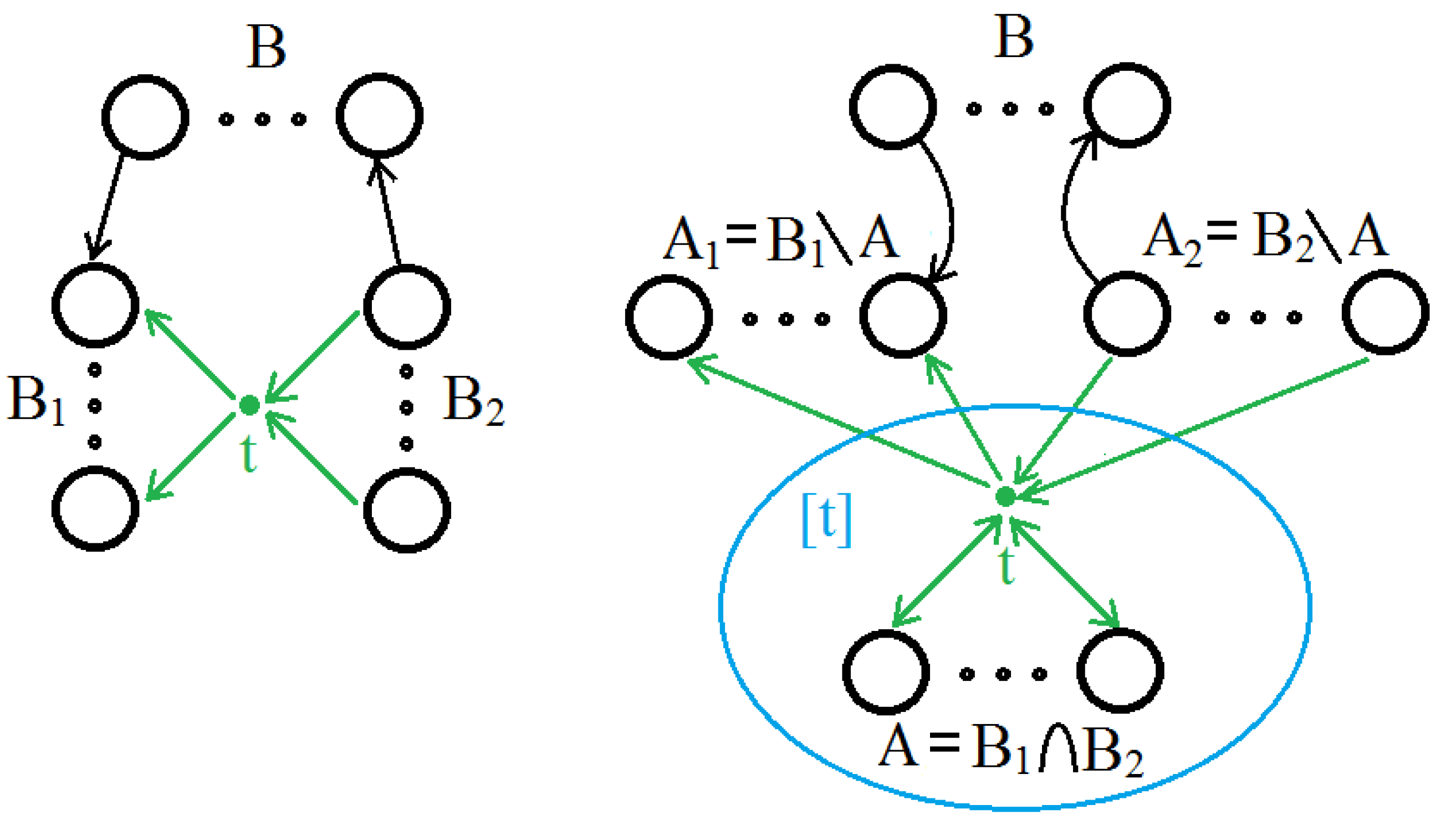
4. Recurrent Algorithm for Class Allocation Cyclic Equivalence

This section provides one of the algorithms for converting a digraph into an acyclic digraph by allocating cyclic equivalence classes in it. There are different algorithms to solve this problem, see for example [12,28], etc. In this section, we show sequential algorithm in which at each step new vertex and arcs connecting it with previously introduced are added to the digraph. This algorithm was convenient to deal with protein networks in numerical examples [29,30].

Let us say that two vertices of a digraph are cyclically equivalent if they are included in any cycle contained in it. On the set of cyclic equivalence classes (clusters), a partial order relation is defined $v⪰w$, if there is a path from the cluster v to the cluster w. We define a zero-one matrix $\left|\right|a(v,w)\left|\right|$ by the condition $a(v,w)=1⟺v⪰w$. Then, the algorithm for determining the set of clusters and the matrix a, specifying the partial order ⪰ on it, is based on the following recurrent procedure [29].

Let all vertices in the original digraph be numbered: $1,2,\dots ,n$. At step 1, a single cluster is constructed consisting of a vertex 1 and a partial order matrix a, consisting of a single element $a(1,1)=1$. Suppose that at step $t-1$, clusters and a matrix specifying a partial order ⪰ between them are given. Then, at the step t, the vertex t and the good arcs connecting this vertex to the already specified clusters are added. Then, in a digraph consisting of clusters constructed at step $t-1$ and paths between them, after adding a vertex t and good arcs connecting it to already constructed clusters, sets of clusters $B_1,B_2,B$ are determined (see Figure 6, left). The set $B_1$ contains clusters into which there is a path from the vertex t. Similarly, the set $B_2$ contains clusters from which there is a path to the vertex t. All other clusters fall into the set B, and from them there can be paths only to the clusters of the set $B_1$ and paths can exist in them only from clusters of the set $B_2$ (see Figure 6, left). Then, at step t, a new cluster $\left[t\right]$ is built, consisting of the vertex t and the clusters of the set $A=B_1\cap B_2$, and the paths between the remaining clusters are shown in Figure 6, on the right. Then, the matrix a of partial order ⪰ is defined by

Table 1. Algorithm of transition from step $t-1$ to step t for a matrix of partial order a.

Matrice Partial Order	Clusters Set ${\mathit{A}}_1$	Clusters Set $\left[\mathit{t}\right]$	Clusters Set ${\mathit{A}}_2$	Clusters Set B
clusters of set $A_1$	meanings on step $t-1$	0	0
clusters of set $\left[t\right]$	1
clusters of set $A_2$			meanings on step $t-1$
clusters of set B	meanings on step $t-1$	0		meanings on step $t-1$

. In this table, rectangular sub matrices 0 consist of only zeros, rectangular sub matrices 1 consist of only ones, and rectangular matrices denoted by values at step $t-1$ repeat the corresponding sub matrices of the matrix a at step $t-1$ (see [29]).

As a result of such clustering, the original digraph is transformed into a digraph with a set of cluster vertices. An arc is drawn between two clusters if at least one arc exists between them in the original digraph.

5. Discussions

Thus, the tasks set in the paper are solved by reducing to the problem of the maximum flow and the minimum section. This allows us to use Ford–Fulkerson algorithms [4,5] and their modifications [22,23], which avoid the need to solve NP-problems. To do this, either the arc throughput is determined in a special way, or good arcs are introduced not for the entire acyclic digraph, but for its arcs coverage, which greatly simplifies the task. We also note that the optimization tasks considered in the paper do not always have a single solution. However, the proposed algorithms allow us to obtain some of these solutions.

References

1. Harary, F.; Norman, R.Z.; Cartwright, D. Structural Models: An Introduction to the Theory of Directed Graphs; Wiley: New York, NY, USA, 1965. [Google Scholar]
2. Wasserman, S.S. Models for Binary Directed Graphs and Their Applications. Adv. Appl. Prob. 1978, 10, 803–818. [Google Scholar] [CrossRef]
3. Bang-Jensen, J.; Gutin, G. Classes of Directed Graphs; Springer: Berlin/Heidelberg, Germany, 2018. [Google Scholar]
4. Ford, L.R., Jr.; Fulkerson, D.R. Maximal Flow Through a Network. Can. J. Math. 1956, 8, 399–404. [Google Scholar] [CrossRef]
5. Ford, L.R., Jr.; Fulkerson, D.R. A Simple Algorithm for Finding Maximal Network Flows and an Application to the Hitchcock Problem. Can. J. Math. 1957, 9, 210–218. [Google Scholar] [CrossRef] [Green Version]
6. Cormen, T.H.; Leiserson, C.E.; Rivest, R.L.; Stein, C. Introduction to Algorithms, 3rd ed.; The MIT Press: New York, NY, USA, 2009. [Google Scholar]
7. Cook, W.J.; Cunningham, W.H.; Pulleyblank, W.R.; Schriver, A. Combinatorial Optimization. Wiley Ser. Discret. Math. Optim. 2011, 33, 48–49. [Google Scholar]
8. Potapov, A.P.; Goemann1, B.; Wingender1, E. The pairwise disconnectivity index as a new metric for the topological analysis of regulatory networks. BMC Bioinform. 2008, 9, 227. [Google Scholar] [CrossRef] [PubMed] [Green Version]
9. Sheridan, P.; Kamimura, T.; Shimodaira, H. A Scale-Free Structure Prior for Graphical Models with Applications in Functional Genomics. PLoS ONE 2010, 5, e13580. [Google Scholar] [CrossRef]
10. Georgiadis, L.; Giuseppe, F.I.; Parotsidis, N. Strong Connectivity in Directed Graphs under Failures, with Applications. SIAM J. Comput. 2020, 49, 865–926. [Google Scholar] [CrossRef]
11. Melo, B.; Brandao, I.; Tomei, C.; Guerreiro, T. Directed graphs and interferometry. J. Opt. Soc. Am. B 2020, 37, 2199–2208. [Google Scholar] [CrossRef]
12. Mezic, I.; Fonoberov, V.A.; Fonoberova, M.; Sahai, T. Spectral Complexity of Directed Graphs and Application to Structural Decomposition. Complexity 2019, 9610826. [Google Scholar] [CrossRef]
13. Marques, A.G.; Segarra, S.; Mateos, G. Signal Processing on Directed Graphs: The Role of Edge Directionality When Processing and Learning From Network Data. IEEE Signal Process. Mag. 2020, 37, 99–116. [Google Scholar] [CrossRef]
14. Dokka, T.; Kouvela, A.; Spieksma, F.C.R. Approximating the multi-level bottleneck assignment problem. Oper. Res. Lett. 2012, 40, 282–286. [Google Scholar] [CrossRef]
15. Zwick, U. The smallest networks on which the Ford-Fulkerson maximum flow procedure may fail to terminate. Theor. Comput. Sci. 1995, 148, 165–170. [Google Scholar] [CrossRef] [Green Version]
16. Backman, S.; Huynh, T. Transfinite Ford–Fulkerson on a finite network. Computability 2018, 7, 341–347. [Google Scholar] [CrossRef] [Green Version]
17. Allen, B.; Sample, C.; Jencks, R.; Withers, J.; Steinhagen, P.; Brizuela, L.; Kolodny, J.; Parke, D.; Lippner, G.; Dementieva, Y.A. Transient amplifiers of selection and reducers of fixation for death-Birth updating on graphs. PLoS Comput. Biol. 2020, 16, e1007529. [Google Scholar] [CrossRef]
18. Bulgakov, V.P.; Avramenko, T.V.; Tsitsiashvili, G.S. Critical analysis of protein signaling networks involved in the regulation of plant secondary metabolism: Focus on anthocyanins. Crit. Rev. Biotechnol. 2017, 37, 685–700. [Google Scholar] [CrossRef]
19. Bulgakov, V.P.; Wu, H.C.; Jinn, T.L. Coordination of ABA and Chaperone Signalling in Plant Stress Responses. Trends Plant Sci. 2019, 24, 636–651. [Google Scholar] [CrossRef]
20. Fàbregas, N.; Lozano-Elena, F.; Blasco-Escámez, D.; Tohge, T.; Martínez-Andújar, C.; Albacete, A.; Osorio, S.; Bustamante, M.; Riechmann, J.L.; Nomura, T.; et al. Overexpression of the vascular brassinosteroid receptor BRL3 confers drought resistance without penalizing plant growth. Nat. Commun. 2018, 9, 4680. [Google Scholar] [CrossRef] [Green Version]
21. Bulgakov, V.P.; Avramenko, T.V. Linking Brassinosteroid and ABA Signaling in the Context of Stress Acclimation. Int. J. Mol. Sci. 2020, 21, 5108. [Google Scholar] [CrossRef] [PubMed]
22. Edmonds, J.; Karp, R.M. Theoretical Improvements in Algorithmic Efficiency for Network Flow Problems. J. ACM 1972, 19, 248–264. [Google Scholar] [CrossRef]
23. Arlazarov, V.L.; Dinitz, E.A.; Ilyashenko, Y.S.; Karzanov, A.V.; Karpenko, S.M.; Kirillov, A.A.; Konstantinov, N.N.; Kronrod, M.A.; Kuznetsov, O.P.; Okun’, L.B.; et al. Georgy Maksimovich Adelson-Velsky (obituary). Russ. Math. Surv. 2014, 69, 743–751. [Google Scholar] [CrossRef]
24. Monjurul Alom, B.M.; Someresh, D.; Islam, M.S. Finding the Maximum Matching in a Bipartite Graph. DUET J. 2010, 1, 33–36. [Google Scholar]
25. Tutte, W.T. The method of alternating paths. Combinatorica 1982, 2, 325–332. [Google Scholar] [CrossRef]
26. Pemmaraju, S.; Skiena, S. Computational Discrete Mathematics: Combinatorics and Graph Theory with Mathematica; Cambridge University Press: Cambridge, UK, 2003. [Google Scholar]
27. Tsitsiashvili, G.; Osipova, M.A. Cluster Formation in an Acyclic Digraph Adding New Edges. Reliab. Theory Appl. 2021, 16, 37–40. [Google Scholar]
28. Tarjan, R. Depth-first Search and Linear Graph Algorithms. SIAM J. Comput. 1972, 1, 146–160. [Google Scholar] [CrossRef]
29. Tsitsiashvili, G. Sequential algorithms of graph nodes factorization. Reliab. Theory Appl. 2013, 8, 30–33. [Google Scholar]
30. Tsitsiashvili, G.; Kharchenko, Y.N.; Losev, A.S.; Osipova, M.A. Analysis of Hubs Loads in Biological Networks. Reliab. Theory Appl. 2014, 9, 7–10. [Google Scholar]
Figure 1. Unrelated stars G 1 1 , G 1 2 , G 2 1 , G 2 2 , M = N = 2 , m = n = 6 .
Mathematics 10 00045 g001
Figure 2. A strongly connected digraph constructed from the stars G 1 1 , G 1 2 (right).
Mathematics 10 00045 g002
Figure 3. A strongly connected digraph constructed from the stars G 2 1 , G 2 2 (right).
Mathematics 10 00045 g003
Figure 4. Introduction of M + N 1 additional arcs.
Mathematics 10 00045 g004
Figure 5. Introduction of max ( m ( M 1 ) , n ( N 1 ) ) good arcs.
Mathematics 10 00045 g005
Figure 6. The algorithm of transition from step t 1 to step t for clusters.
Mathematics 10 00045 g006