1. Introduction
Global processes of transformation have begun in recent years. The actuality of solving the tasks of effective management of structurally complex sociotechnical systems has increased significantly. The concept of the value of objects (assets) included in such systems “presses up” the value of assessments and the significance of decision-making becomes determining, but the definition of this “value” remains more an art than a scientifically based methodology. Intuitively, with limited resources (of all kinds), it is necessary to aim to use these resources in the most rational way. However, to develop a rational solution, it is necessary to learn how to assess the results of the targeted activities of the system, how to apply them to the tasks set and learn the costs associated with each solution. To make a comparison, you need to learn how to measure certain quantitative features that characterize the functionality of an individual object and the entire complex sociotechnical system. You also need a “tool” that allows you to assess the result. Since the task lies in choosing the best of the compared options for the growth and development of the system, first, it is necessary to learn how to measure the quality of decision-making. The quality of any solution becomes apparent only in the process of its implementation (in the process of target operation of a managed object or system). Therefore, the main objective is the assessment of the quality of the solution by the effectiveness of its application. Thus, to reasonably choose the preferred solution, it is necessary to measure the effectiveness of the target function of the managed object or system versus its compared variants [
1] in conditions of existing uncertainty and risk.
The comparison of options and decision-making directly depends on the competence of decision-makers (DM), that is, on their ability to comprehensively assess the risks associated with the functioning and development of the system. To ensure a well-founded choice of DM, we propose using decision-formers (DF), which as a rule, are analytical tools based on mathematical methods. These can be found in Kantorovich’s “simplex method” [
2] on through to modern machine-learning methods, neural networks [
3,
4,
5], methods of reference vectors [
6], genetic algorithms [
7], etc.
There are several classes of decision-making tasks:
deterministic, which are characterized by a one-valued connection between the decision-making and its outcome, aimed at building the “progress” function and determining the stable parameters at which the optimum is achieved;
stochastic, in which each decision made can lead to one of many outcomes occurring with a certain probability. Usually, it uses simulation programming methods [
8], game theory [
9] or other methods of adaptive stochastic management [
10] to choose the optimal strategy in view of averaged, statistical characteristics of random factors;
in conditions of uncertainty, when the criterion of optimality depends, in addition to the strategies of the operating party and fixed risk factors, and also on uncertain factors of a non-stochastic nature, an interval mathematics [
11] approach, or approximations in the form of fuzzy (blurred) sets [
12,
13], are used in decision-making.
The latter case involves processing the views of independent experts [
14,
15]. Despite the wide application of expert systems in practice, the fairness of using certain methods of analysis remains incomprehensible for many DM, especially when the results are contrary to “common sense” (in their understanding) [
16]. So, developers have to formulate and uphold certain principles, without which the automation of methods adopted in expert systems becomes unacceptable.
Often, expert assessment procedures are based on the method of processing matrices of pairwise comparisons of various alternatives, known as the Saaty algorithm (or hierarchy analysis method) [
17]. It is quite widely used despite criticism [
18,
19,
20] and the lack of a one-valued solution to several research issues.
Firstly, with large dimensions for the pairwise comparison matrix, the number of comparisons for each expert increases to , where is the number of alternatives considered. Problems arise with the “poor-quality” filling of the comparison matrix by experts and the “insufficient” quality scale used in the method.
Secondly, not all experts can compare all proposed alternatives in pairs, and so some pairwise comparison matrices will remain unassessed (NA). Partially, this issue was solved by Saaty with the development of the method of analysis of hierarchies and the method of analytical networks, but the latter contains several strong assumptions that impose restrictions on its application [
21,
22].
Thirdly, as a rule, there is no “reference” alternative; the remaining assessments are obtained by converting
, which is used, for example, in combinatorial methods for restoring missing data [
19].
Fourthly, when summarizing the opinions of experts and moving to a common matrix of pairwise comparisons, values with significant variation appear in the same cells, which necessitates working with the assessments set in the interval scale [
23].
Finally, in the case where the alternative to comparison is not the object itself, but instead a scalar method is determining risks, then the task of selecting objects is reduced to assessing the weights of factors affecting the integral risk. As a result, a complex problem of analyzing the risks of objects arises, which can be solved by minimizing the integral risk [
24].
2. Smart Expansive System
Complex systems theory (synergy) uses nonlinear modeling and fractal analysis for forecasting. In the last decade, such innovative areas as theoretical history and mathematical modeling of history, based on a synergistic, holistic description of society as a non-linear developing system, have been actively developing (V. Glushkov, B. Onyky, N. Zhigirev, S. Kurdyumov, D. Chernavsky, V. Belavin, S. Malkov, A. Malkov, V. Korotaev, D. Khalturina, P. Turchin, V. Budanov).
Modern complex sociotechnical systems are characterized by distribution in space, a large variety of objects included in their composition and interaction of various types of objects, a heterogeneous structure of transport and technological chains, unique conditions for influencing individual objects and the system as a combination of risks of various natures. If the stability of the functioning of such complex systems means the implementation of their development plan with permissible deviations in terms of volume and timing of tasks, then their management is reduced to minimizing unscheduled losses in emergency situations and taking measures to anticipate them, that is, for the analysis, assessment and management of associated risks.
The concept of management of such systems strives to achieve an optimal balance between the cost of the object, associated risks and performance indicators, based on which economic goals are formed and the use of the object is ensured in such a way that it creates added value. In general, optimal profit-oriented management strikes a balance in the reallocation of available resources (material, human and information) between “productive activities” and “maintaining development potential”.
The above is described most closely by models of interaction between a developing object and its environment, such as in the model of self-perfecting developing systems of V. Glushkov. He introduced a new class of dynamic models based on nonlinear integral-differential equations with a history [
25]. He also developed approaches to modeling the so-called “self-perfecting systems” and proved theorems on the existence and uniqueness of solutions, describing their systems of equations [
26].
However, it should be noted that the name “developing”, applied to the class of systems in question, is not quite correct and contains some ambiguous interpretations. The growth of the system may not be accompanied by its development (for example, improving the science of creation and design, instructions for the manufacture or use of the product) and vice versa (for example, expectations of a quick practical return on basic science). Usually, growth and development are combined, there is a smooth or uneven change in the proportions between them and some “equilibrium” state with the external environment occurs (or does not occur).
In parallel with the work of V. Glushkov, works on Scientific and Technical Progress (STP) have also begun in specific industries. Examples are the studies of B. Onyky and V. Reznichenko [
27,
28], who laid the foundations for the theory of potential systems, and the early works of N. Zhigirev [
29]. Based on biophysical and economic models, they proposed a practical new version including integral-differential equations that describe the process of producing, introducing and forgetting knowledge in production cycles due to the transition to other scientific and technological foundations. They demonstrated the cyclical nature of capacity-building and the need to develop complex systems (health, education, industrial safety systems, ecology and other infrastructure projects by generation).
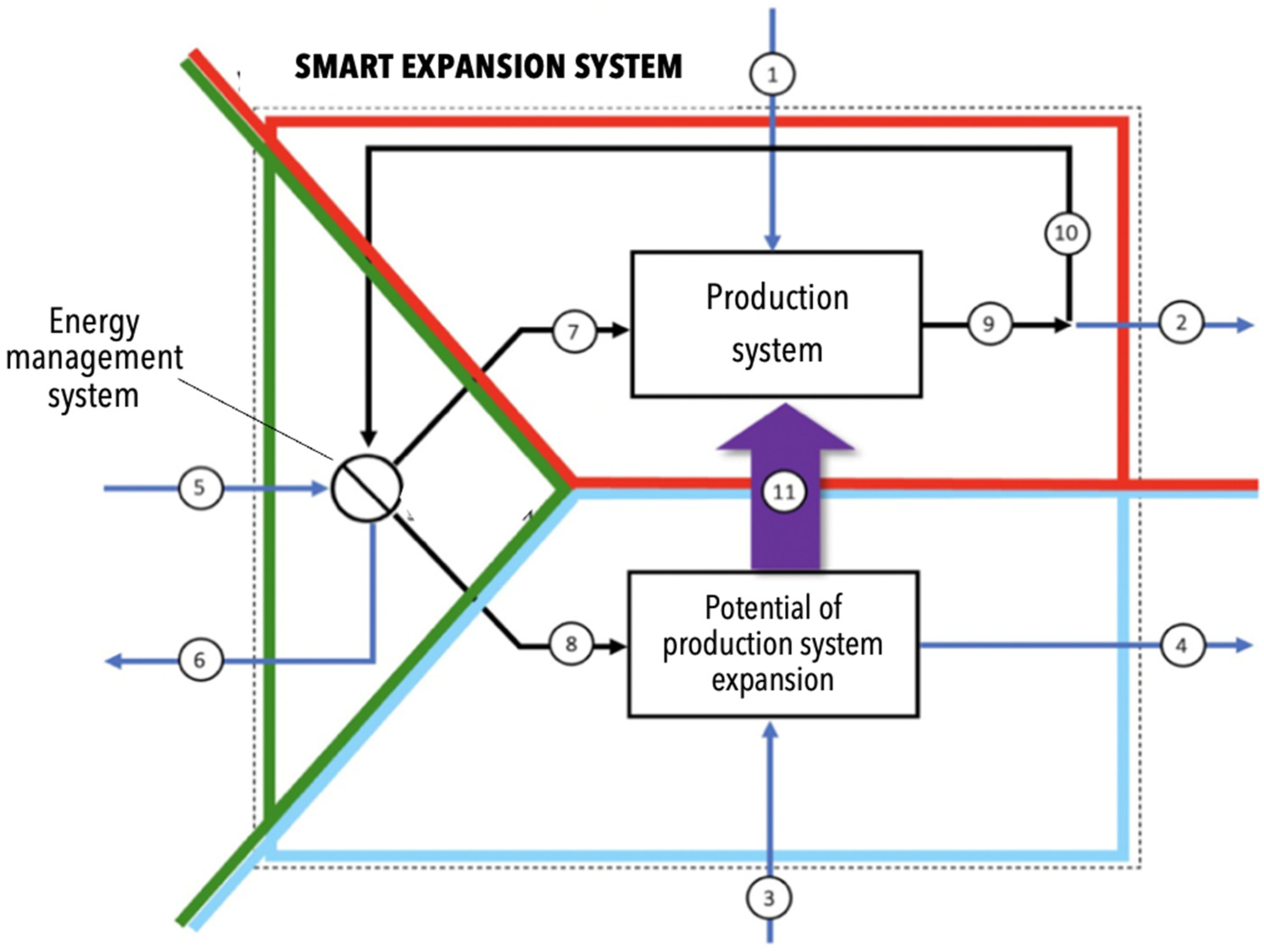
Our understanding and development of the aforementioned models compel us to introduce into consideration a class of so-called “smart expansive systems,” consisting of three subsystems (
Figure 1).
The smart expansive system (SES) is an open system that may be growing or developing, or simultaneously both growing and developing (when, for example, objects of different “generations” are included in it). Sometimes the growth of the system is accompanied by “flattening” (flatlining at the same level of development) and degradation in its development. The SES is open since it needs to effectively allocate the necessary resources from the external environment, possibly “cleaning” them before use (including the human resource), and remove biowaste.
The production subsystem is assessed by the reproduction rate multiplier at a conditional minimum development potential. Below this minimum (critical mass of potential), the growth and development of the SES are impossible in principle. The potential catalytic function describing this multiplier in the limit is an asymptotic curve with saturation (like a logistic curve), although potential inhibition is also possible since the production subsystem occupies the space of a common SES. This behavior is similar to the flow system of the “Brusselator” (an intensively working conveyor) when initial substrates flow out of it, which do not have time to react with the catalyst, despite their sufficient amount [
30].
The production subsystem serves to measure the success of expansion, determined, for example, by the volume of useful products produced by the system.
The subsystem of the expansion potential of the production is intended for catalytic management of the produced forms and resources (sometimes measured by money with a dual structure—the cost of renewing matter and the cost of maintaining information in the broad sense of the word).
The energy management subsystem is actually a two-circuit resource management system (financial and temporary) between production and contribution to infrastructure projects.
In
Figure 1, the externally directed energy flow (5) is distributed by the control subsystem to the production subsystem (7) and goes to the expansion potential subsystem for the production of knowledge and improvement of technologies, which are “recipes” for the preparation of products (the so-called flow to the development of “infrastructure”). From the external environment, the expansion potential subsystem also receives additional information on new knowledge, inventions and technologies (3) and has a catalytic effect on the production subsystem (11). The production subsystem, in turn, receives from the external environment a flow of “purified” semi-finished products (1) for further expansion. In the process of expansion, there is inevitably a partial forgetting of information due to various causes, including the physical death of the carriers of the original thought forms (4), which causes a weakening of the expansion potential of the entire system.
There is an outflow (2) of products from the production subsystem to the external environment, including unused semi-finished products, waste from the assembly of products, etc. Purified from (2), the flow of energy from the results of labor to the production subsystem and the results of sales of products on the market supports the functioning of the regulatory subsystem. In the latter, over time, it is possible to disperse energies (6) not yet distributed among subsystems that can cause, under certain conditions, a collapse of the management system.
Leaving beyond the scope of this article a detailed description of external and internal interactions, let us dwell a little more on the features of a deterministic and stochastic approach to modeling smart expansive systems.
2.1. Deterministic Model of Smart Expansive System
For the deterministic case, the SES is described by a two-parameter model for time (1) and for the proportions of the energy distribution (3). The first equation describing the system is in a sense autonomous:
where
is the volume of the “production subsystem” measured by the number of products;
—the additive of linear part—maintains the production technology and requires linear costs (in economics, for example, these are depreciation costs);
is a linear production function of a useful subsystem with the parameter
;
is the proportion of energy distribution from newly created forms
;
;
is the coefficient of the scale of production losses, where as a rule,
is performed;
beforehand is the set amplifier of the production of forms due to reading “the correct information” (e.g., instructions for assembly), with information as a catalytic function;
is a quadratic term that considers the limited “semi-finished products” and the competition of finished “products” in the surrounding world.
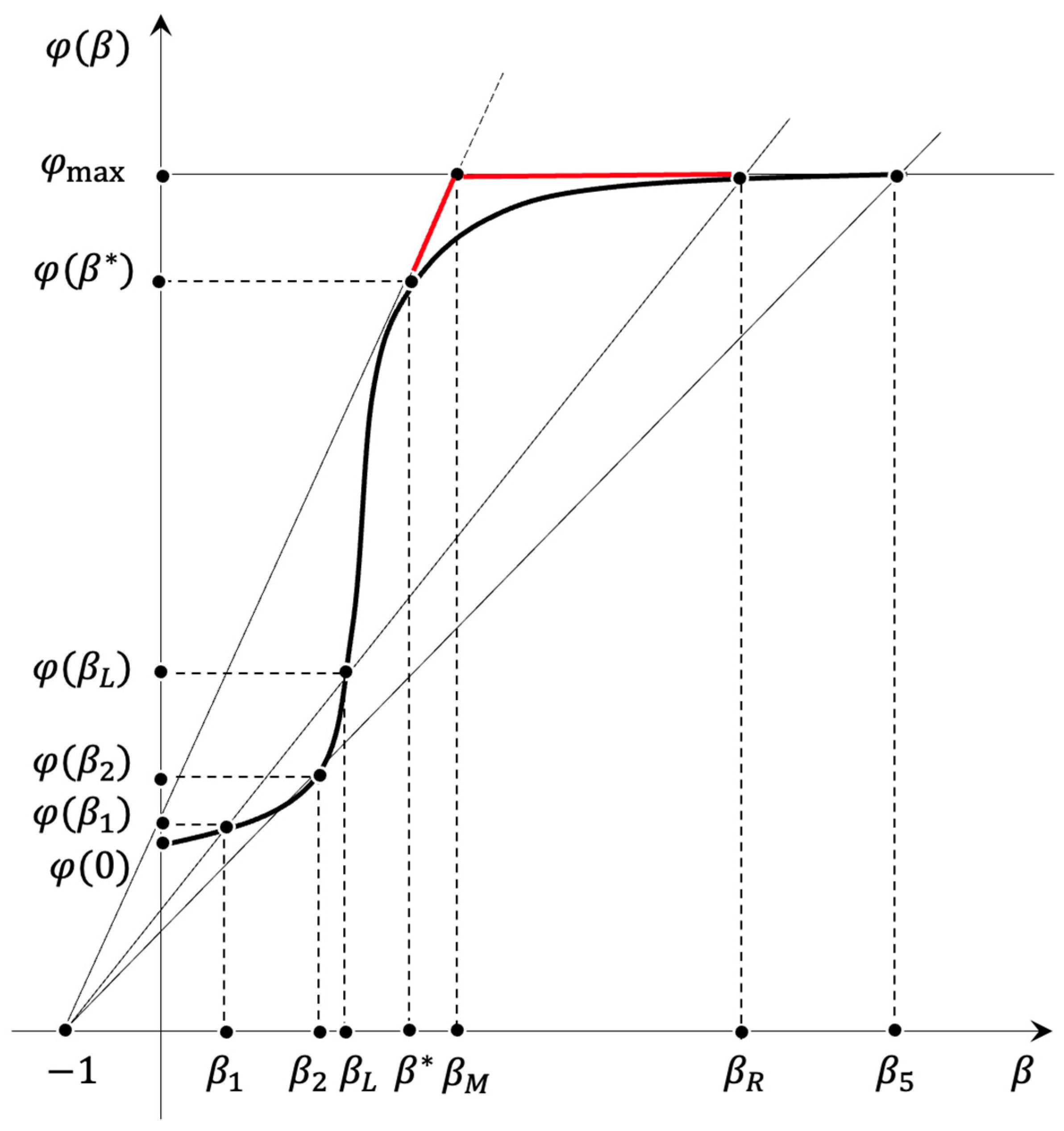
The function
takes the form of a logistic curve (
Figure 2), which is generally unnecessary if the requirements of positive constrained monotonicity are met. This function can have breaks of the first kind. The final form of the function
with the argument
is also determined by the degree of necessary detail for the calculation.
Segments on the abscissa axis , and if are the area of degradation of the smart expansive system. Accordingly, the segments , and if are the area of its growth (development). Moreover, the expansion of the system begins only from (on the segment grows, and on the rest, it only decreases). Above the limit value it makes no sense to look for a solution, although already at the point the system begins to degrade actively.
The type of logistic curve is selected so that in the segment the efficiency of the productive subsystem is extremely low (this is the field of low-skilled labor and individual potentially breakthrough ideas in science). The segment corresponds to mass production using the available knowledge and skills. The optimal is inside , while at , science is not sufficiently developed and highly-demanded, and at , science is “too much” and the results of scientific research simply do not have time to be introduced and mastered in the production subsystem.
The point
in
Figure 2 corresponds to a situation where all resources are spent exclusively on the growth of the production subsystem. The potential of such a system is low due to permanent losses that can be avoided if there is the potential to anticipate and manage emerging risks.
The section shows that if the funds assigned to study and counteract threats and risks are small, then the return on such research and activities is less than the resources assigned to them. Information collection for low-level investigation of internal and external threats does not allow for an adequate assessment that improves the quality of decision-making in most cases.
On the segment , the contribution to the development potential begins to give a positive return; however, the so-called “self-repayment” level of the costs of developing the “potential” of the system will be achieved only at the point . Therefore, it is advisable to consider this point as a point of “critical” position. The reduction of the potential to the level threatens a situation where “due to the circumstances,” the “survival strategy” will be economically suitable—that is, taking the strategy of completely eliminating the cost of solving the tasks of prediction and anticipation of threats and risks, and ensuring reproduction only by increasing low-efficiency capacities in the production subsystem .
The optimum is reached at point
. This point has a certain sense to it. If resources for the development of potential are given “excessively”
, then the funds
are incorrectly removed from the current reproduction and a situation arises where disproportionate efforts are spent on studying and counteracting many risks that the developing system may never face. The optimum does not depend on the values
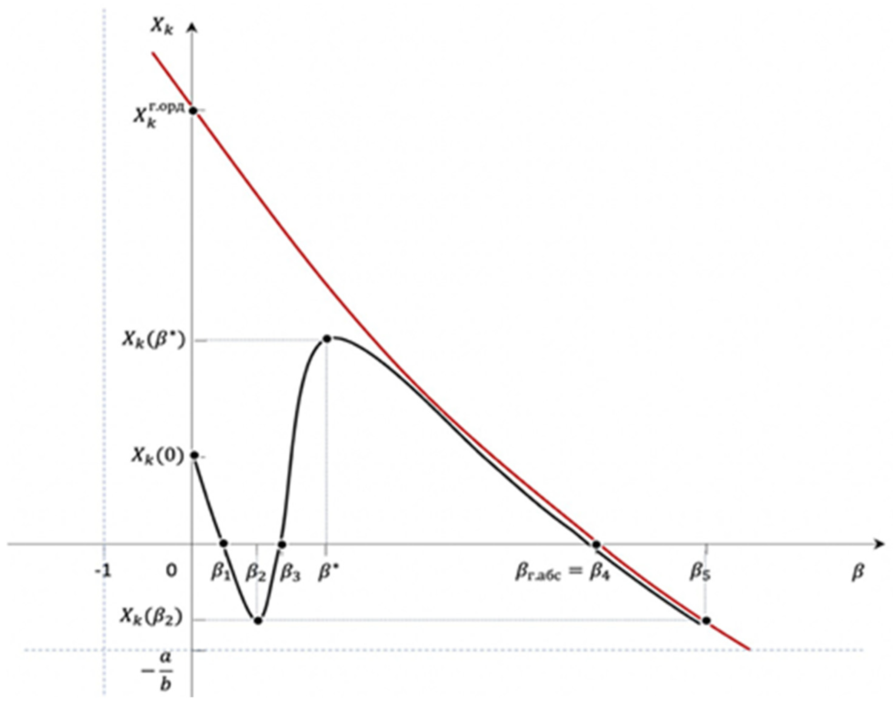
. There may be cases where
is so large that even with an optimal solution, the system does not develop, but degrades. The condition of non-degeneracy of the decision is the presence of positive ordinates in
(
Figure 3).
Generally, for the segment only the overregulation and excessive formalization of management of a system can do much harm, and for the segment there is a situation where the costs of searching for an existing solution are so great that it is preferable to receive it anew.
In
Figure 2, with
along the abscissas axis and
along the ordinate axis, we draw half-lines from the point
crossing the graph’s
. The position of the half-line is set at
with a tangent
to the abscissa axis
and crosses over the ordinate axis at point (0,
).
The position of the upper touch of the half-lines corresponds to the coordinate (
for which the following is performed
With a fixed and , an initial (next to zero deformation of the space of forms) and an asymptotically final volume , solutions can be represented in the form of a logistic curve.
If and , then .
Let us find out how the parameter influences final productivity, which means a stable equilibrium state of .
Considering the difference scheme, we define the final growth graph with a step : , where = .
The final graph
, taking into account the compression of the graph
by
and the displacement by the value
vertically downward, followed by division by the value
, is shown in
Figure 3.
The second equation describes the dynamics of the laws of functioning of the system, by which
is created
Here, is the initial state. The regulator describes the loss of knowledge, but corresponds to the complication of laws for new unknown management functions (“emergence”) that are not available in subsystems.
We define the maximum
where the parameter
.
Making a replacement
we get the final solution of the following form
where parameter
is searched for as the maximum value from the above range.
Maximum
is reached either at the edges of the segment or in one of the local minima. So, in
Figure 2, on the asymptote,
,
is performed.
This allows us to obtain a four-parametric model
of the initial quasi-linear growth.
Here, it is possible to give an explicit formula for
and it is possible to limit this to a simplified form
In conclusion, we confirm that
gets into the segment
, i.e.,
The solutions are either
or
depending on
The first bracket in (18) is the inability to create anything —in this case, it acts as a criterion for the feasibility of expansion in general.
The second bracket, subject to
is a criterion for achieving the desired performance
in the production subsystem.
The positivity of their work guarantees
Otherwise, the optimum is on the left edge
, i.e.,
However, there are unique systems, the value of which depends solely on the capacity of the producer. When the potential is high and its assessment is not underestimated relative to “fair”—i.e., —the second bracket is carried out, even at and with a lack of competition from other producers .
The presence of two optimal solutions (by the number of products) and (by the “mind”), determined through the constant in (22), means that optimal will be refusal of the gross product in favor of maximum use of the expansion potential, that is, production with the “optimal” margin of “possible use” of the manufactured products (multifunctionality).
Despite the counter nature of the described model, this gives the idea that threats and risks can be considered as “anti-potentials” of development (i.e., they are retardants of the reproduction rate of the entire system). To model a real system, it is necessary to analyze the “raw” process data and then synthesize them into a meaningful structure explaining the process under study.
2.2. Stochastic Linear Growth Models of Smart Expansive System
2.2.1. Model of System Growth Taking into Account the Effect of Random Perturbations of System Productivity on the Speed of Its Reproduction
The model takes into account that in the “quasi-linear section” of the expansion of the system, not only is the speed of expansion important but also the dispersion of the process. At the same time, the “volatility” of the process itself plays a greater role than the profitability of the “production subsystem”.
Despite an increase in the “average” amount of product from each element of the system, each element is individually characterized by a limited time of effective operation. Moreover, the indicator of “population mortality” under natural restrictions on mathematical expectation is mainly influenced by the magnitude of the variance. Therefore, for example, in economics, where processes with mathematical expectation values of several percent are studied, the variance values themselves appear in the definitions of “risks”.
Here, it is extremely important to note that to assess the values of mathematical expectation and variance, they are quantified at the starting point of time based on group assessments. It is further hypothesized that these assessments obtained for the group can be used to predict the trajectories of each element of the group separately. This is a very strong assumption since the model claims, firstly, that the obtained assessments will remain constant for the entire forecast time, and secondly, it is established that each element at any time behaves in the same way as some element at zero point in time. Such assumptions are true, generally speaking, only for ergodic processes. Yet, not all the processes described by the model in question are ergodic. In systems consisting of elements of more than one type, the need to consider such “risks” is greatly increased, and these “risks” themselves are much higher.
2.2.2. Model of Impact of Capital Fluctuation on System Growth
This model is not related to the properties of the system itself, but to the level of fluctuations in the parameters (influencing factors) of the external environment (fluctuations in the level of corruption, changes in tax legislation, etc.). The most likely values for the number of elements in such a model are always less than its average value. A certain value is introduced as the threshold of state criticality.
If the current value is lower than the critical value, the probability of ruin increases sharply. It is important to note that with the increase in time, critical values also increase.
Moreover, if the fluctuation amplitude of the distribution variance assessment is large and the mathematical expectation and initial value are sufficiently small, then the probability of degeneration of the system tends to one.
Thus, on average, external fluctuations accelerate the growth of the system, but the payment for such accelerated growth is an increased probability of its degeneration (a decrease in the mathematical expectation of its degeneration time), and since the expansion process is multifactorial, but the “history” of the behavior of such a system (as is the case, for example, in mass service systems), as a rule, is not, it is essential that rather than conducting an analysis based on statistics from past observation periods, instead, a synthesis of the risk of functioning of the “smart expansive system” is carried out.
3. Smart Expansive System’s Risk Synthesis
Regarding risk, the concept of “synthesis” is currently hardly used in contrast to the concept of “analysis”. However, it is necessary to understand that risk analysis is characteristic of systems in which risk realization events occur often enough to apply a well-developed apparatus of probability theory and mathematical statistics. This approach works in insurance, for example, in the theory of reliability, when we deal with the flow of insurance cases, accidents or breakdowns. Yet, when it comes to ensuring safety in an era where the main characteristic is constant unsteadiness and variability, it is possible to do this only through the synthesis of risks, developing automated advising systems that become complicated as they develop tips for professionals (DF) or replacing professionals with highly intelligent robotic systems. The risk from the concept of “analytics” in this case is becoming “synthetic”.
As the analysis of integrated assessments of the state of complex objects and systems used in system studies shows, generalized risk criteria (indices) are widely used. There are additive (weighted average arithmetic) and multiplicative (weighted average geometric) forms of these:
arithmetic (smoothing “emissions” of private risk indicators) ;
geometric (enhancing negative “emissions” of private risk rating) ;
geometric anti-risk .
Weight coefficients
of partial estimates
satisfy the condition
Real numbers (private risks) take values from the interval between zero and one.
For smart expansive systems, the most acceptable form of risk representation is geometric anti-risk [
31], which satisfies the main a priori requirements underlying the risk approach to the construction of a nonlinear integral assessment of
, namely:
- 1.
smoothness—the continuous dependence of the integral assessment and its derivatives on private assessments:
- 2.
limitation—limits of the interval of change of private
and integral
assessments:
- 3.
equivalence—the same importance of private assessments and ;
- 4.
hierarchical single-level—aggregate only the private assessments of that belong to the same level of the hierarchical structure;
- 5.
neutrality—the integral assessment coincides with the private assessment when the other one takes the minimum value:
- 6.
uniformity .
The geometric anti-risk derives from the concept of “difficulties in achieving the goal” proposed by I. Russman [
31], and is the “assessment from above” for the weighted average arithmetic and weighted average geometric risk.
Risk as a measure of the “difficulty in achieving the goal,” and assesses the difficulty of obtaining the declared result with the existing resource quality assessments () and requirements for this quality (). The concept of difficulty in achieving a goal with a given quality and given requirements for the quality of a resource and the result follows from the considerations that it is more difficult to obtain a result of a certain quality when there is a low quality of the resource or a high requirement for its quality.
For general reasons, the difficulty of obtaining result should have the following basic properties:
when should be maximum, i.e., equal to one (indeed, the difficulty of obtaining the result is maximum at the lowest permissible quality value);
if and should be minimal, that is, equal to zero (for the maximum possible value of quality, regardless of the requirements (for ), the complexity should be minimal);
if and should be minimal, that is, equal to zero (obviously, if there are no requirements for the quality of the resource components and is more than zero, then the difficulty of obtaining a result for this component should be minimal).
For these three conditions for , a function of type is allowed.
We also assume that for and 1 for .
The functioning of the reliable system is characterized by the preservation of its main characteristics within the established limits. The actions of such a system are aimed at minimizing deviations of its current state from some given ideal goal. In relation to the system, the goal can be considered as the desired state of its outcome, that is, not only the value of its objective function.
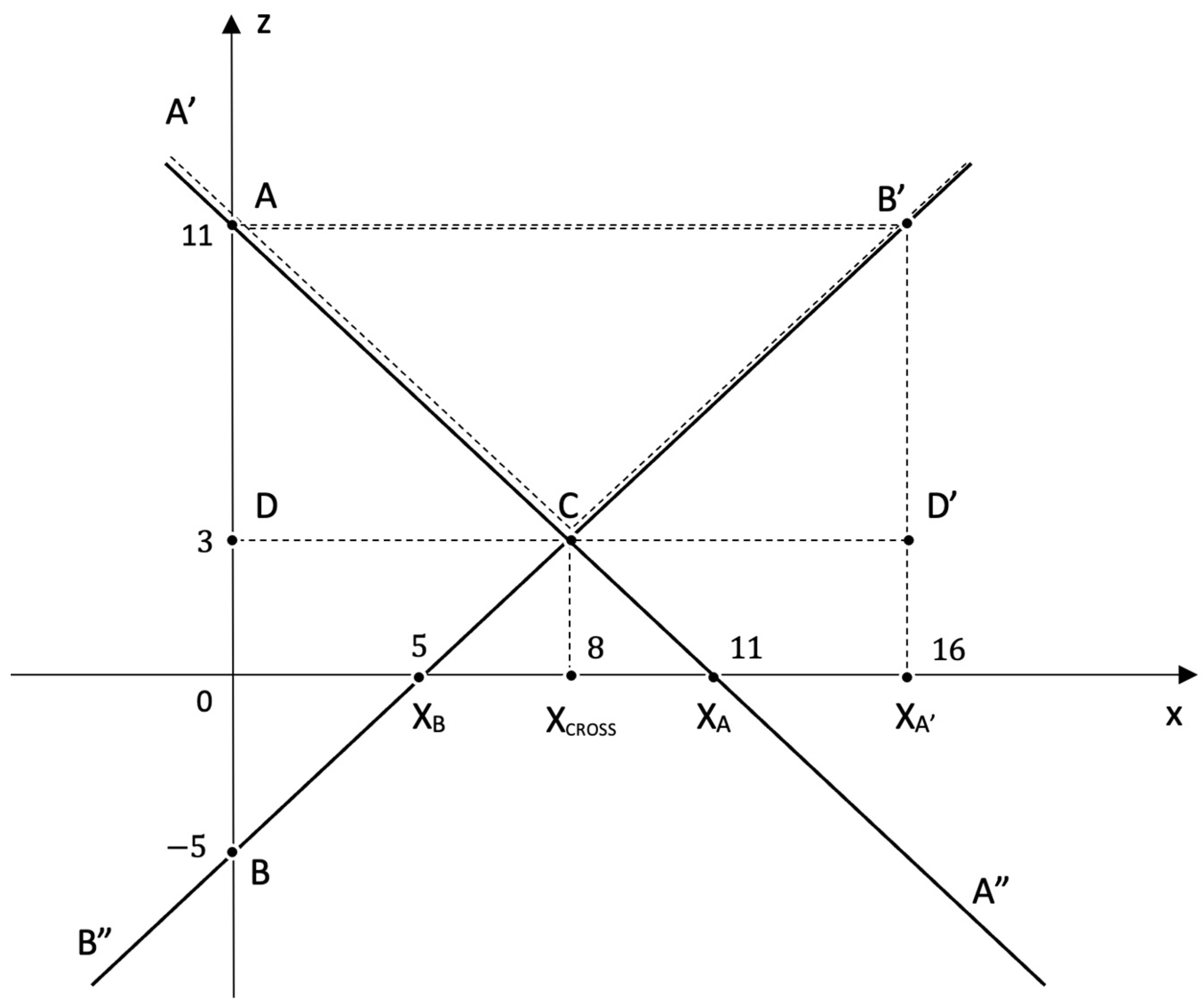
Let us briefly explain the essence of geometric anti-risk. We will consider the system in the process of achieving the goal, moving from its current state to some future result, the quantitative expression of which is
. Let us suppose that the goal is achievable in time
We also assume that there is a minimum speed of movement
to the goal in time and a maximum speed
. It is most convenient to measure the quantitative expression of the result and the time required to achieve it in dimensionless values; to do this, we assume
and
equate to 1 or 100%. In
Figure 4, the minimum and maximum speed trajectories of the system correspond to the
and
lines.
Polyline
is the boundary of the exclusion zone, and for any point
with coordinates (
), to describe the position of the system on an arbitrary trajectory to the goal within the parallelogram
, the distance
is taken as the risk of not reaching the goal:
where
.
We emphasize that the geometric anti-risk satisfies, in addition, the so-called theorem “on the fragility of the good” in the theory of disasters, according to which, “…for a system belonging to a special part of the stability boundary, with a small change in parameters, it is more likely to get into the area of instability than the area of stability”. This is a manifestation of the general principle that everything good (for example, stability) is more fragile than everything bad [
32]. Risk analysis uses a similar risk-limiting principle. Any system can be considered “good” if it meets a certain set of requirements, but must be considered “bad” if at least one of them is not fulfilled. At the same time, everything “good”—for example, the ecological security of territories—is more fragile, meaning it is easy to lose it and difficult to restore.
The continuous function
satisfying the above conditions has the following general form (27):
If in a special case
, then:
which gives an understated assessment of integral risk based on the calculation that the flow of abnormal situations for objects of the system is a mixture of ordinary events taken from homogeneous but different values of
samples.
Since for real systems, risks are usually dependent, we have
where
are the risk connectivity coefficients of the
i-th and
j-th abnormal situations for the objects of the system and
and
are positive elasticity coefficients replacing the corresponding risks. These allow for taking into account the facts of “substitution” of risks, mainly since effective measures to reduce all risks cannot simultaneously be carried out due to the limited time and resources of DM.
The current values of private risks included in the integral indicator (27) are values that vary over time at different speeds (for example, depending on the seasonal factor, the priorities of the solved technological problems in some systems of the fuel and energy complex change significantly).
Private risks are built, as a rule, through the convolution of the corresponding resource indicators—factors of influence that have a natural or value expression. These factors are measured on certain synthetic scales (for example, in the previously mentioned multiplicative Saaty, the pairwise comparison scale), the mutual influences of which should also be studied since they are generally nonlinear and piecewise-continuous.
To obtain assessments of factors of influence, weighted scales must be built. To this end, the authors have developed the so-called “vector compression method” [
33], which is discussed herein.
4. Vector Compression Method: Stationary Method of Incomplete Pairwise Comparison of Risk Factors
When moving from the preference scale to the linear logarithmic scale, the weights of objects
are converted into
, and the matrix of pairwise comparisons of the factors of influence of private risks
is converted into an incomplete antisymmetric matrix
[
21].
The indicator matrix monitors the status of the link network. It takes two values: when the link occurs, and when it is absent , not available). This article deals only with the case of stationary matrices .
An analog of the matrix consistency condition in such a statement is the elements of the antisymmetric error matrix
:
For correlation, matrices for all .
4.1. General Properties of Transformations of Antisymmetric Matrices
Let us introduce the basic designations:
—maximum value of elements of matrix , for which indicator function (maximum on line );
—minimum value of elements of matrix , for which indicator function (minimum on line );
—maximum value of matrix elements , for which indicator function (maximum by column ).
The essence of the transformation of the matrix with the parameter consists of an element-by-element reduction by of all elements of the -th line and an increase by of all elements of the -th column of the antisymmetric matrix .
Transformations ,…, differing only by the parameter with the constant we will call the same type.
The vector compression process is illustrated in
Figure 5, in which the abscissa axis is the parameter
and the ordinate axes are two deposited graphs of crossing straight lines
and
with the resulting function
of the following type:
Moving to the point of intersection of the lines with the coordinate , we reduce the modulus of the difference between and .
Since the first addend does not depend on , the result depends on the sign under the module. At the point of intersection of , the module is zero.
Transformation properties:
- 1.
Zero neutrality: regardless of the type, zero displacement leaves the matrix unchanged
- 2.
Absorption: two transformations of the same type are added together
- 3.
Rearrangement: two adjacent transformations, regardless of their types, can be rearranged
- 4.
Cyclicity: regardless of
the following is executed
Used to line up the final displacement parameters
- 5.
Convolution of sequences by permutation and absorption:
is provided by permutation of transformations (by property 3) of the first type to the left with absorption (by property 2). The same procedures are then implemented for the second and subsequent types.
From properties 1–5, it follows that at any time , the state of the matrix is determined by the initial matrix and accumulated sums for the same type of transformation, while the order of application of transformations of various types is not important.
4.2. Transordinate Vector Compression Method
The choice of displacing
influences the matrix
with transformation
.
The values and are aligned.
Definition 1. The first norm is the maximum of the matrix if Gi,j = 1.
Two lemmas of convergence are true.
Lemma 1. (by lines). If is the only maximum, at which , then . (by line ).
Lemma 2. (by columns). Let the single maximum be reached on element . Then, the decrease is achieved due to the conversion (by the column ).
Definition 2. The second norm is defined as the sum.
By virtue of Lemmas 1 and 2, the process of lowering the first norms converges. If the first and second norms are zero, the matrix becomes zero, and the matrix becomes consistent and is fully determined by the value of the accumulated sums taken with the inverse sign.
For uncoordinated matrices , the convergence process described in Lemmas 1 and 2 results in final states other than the zero matrix . The second norm becomes zero, and the first norm becomes equal to the value , which in the future we will call the consistency criterion of the matrix .
Now, let us consider the set of lines for which is . Each line has at least one maximum and at least one minimum . The remaining elements of matrix for which is executed may be temporarily discarded.
We create oriented graph from . We will assume that the maxima are the entry points to the top and the minima are the exit points from . As a result, will have one or more cycles, and the cycles can be inserted into each other. The obtained graph is not necessarily connected, nor does it necessarily contain all the tops of the graph .
Each cycle is similar to the known task in the theory of antagonistic games—the game “rock-paper-scissors”, where the criterion of consistency plays the role of a “bet” in one game. With a small bet, the game is quite harmless. The price of the game is zero, and there is a Nash balance—it is absolutely random, not subject to any algorithm and there is proportional use of all three strategies. With a large bet (not comparable to the smaller capital of one of the players), a “tragic” outcome is possible—no one will give credit to the loser to “recover his losses”. How to reduce the game’s bet? With large consistency criteria , an unsolvable situation arises.
The first way out—as in the method of analyzing hierarchies, is to abandon the results of uncoordinated expertise.
The second way out is to abandon some grades from , and instead of accept . It is necessary to break some kind of cycling connection, without destroying the connectivity of the remaining graph . By breaking the cycle with , after recalculation there will be a smaller value .
The third way out is that communications remain the same: and new is not formed, but matrix weights ”recover”, as specified in top set . This is the best way to ensure it has counted —the maximum value “preceding” the current value of that does not participate in the construction of .
Let be executed for . In fact, you can limit yourself to a non-zero minimum level of . Yet, when , matrix must be subtracted from matrix , on which the mask from elements of a positive multiplier is imposed on elements from . Thereby, the new matrix of will have the criterion of coherence .
After that, it may be necessary to recalculate the “non-critical” (not included in the top set ) “accumulated sums” of lines and form a new matrix . If this is for a new , will be executed. Let us continue the procedure as described above. If on any step , the step is summarizing and parameter decreases to .
4.3. Gradient Vector Compression Method
The presence of two equivalent methods (line
and column
) serves as the basis for a gradient variant of realization of the vector compression method. As can be seen from the matrix transformation definition itself, optimal compression at each time point
is not necessary for success; it is only necessary to set the correct direction. To avoid searching each iteration for the “best pair” by the displacement value (
Table 1), one may wish to reduce the displacement value several times.
First, by computational experiment, and then, theoretically, it was possible to show for matrices that an increase in the divider in the displacement value by a factor of Q = 1.5 turned out to be more effective. This allows the maxima and minima of the matrix to be recalculated once every N iterations.
As a result, the algorithm of the gradient method of vector compression is reduced to the following successive steps:
- 1.
Calculate local maxima and minima by lines.
- 2.
Recalculate .
- 3.
If , transition to item 1.
Otherwise:
- 4.
If > is a correction of = , the previous can be left.
Transition to item 1.
Otherwise:
The specified accuracy has been achieved.
In these steps, is a measure of the inaccuracy of the definition of a gradient of logarithms of weights, while is the required accuracy of the decision.
Obviously, inequities are being fulfilled
4.4. Hybrid Methods for Partial Pairwise Comparison with Fuzzy Information
The tool discussed in
Section 4.3 is applicable for operation with one decision matrix (filled with half-significant elements [
23]). To work with matrices of large dimensions, various methods of aggregating assessments are needed [
34]. This is significantly observed in two extreme cases—when the number of experts
is large, and when the number of objects of comparison
is large. In either of these scenarios, a significant chunk of the resources will be spent on checking non-zero values of the indicator matrix
. Therefore, we propose representing generalized matrices in the form of “lists” of non-zero elements by lines
, or in the form of a multilayer regular neural network (NN), which implements the calculation of local maxima
and minima
by lines.
In this case, the calculation of “lists” can be regularized by the addition of maxima
and minima
into the functions of calculation to take the place of missing communication elements, such as communication with the first elements in the list (element in the first layer of the NN). They are marked in the examples below (in
Table 2, grey on an orange background, and in
Table 3, yellow on a grey background).
It is advisable for a group task to have a regular sub-table of inter-matrix links as the first links, in contrast, for co-scaling tasks, select positive elements straight above the main diagonal. All elements will be non-negative except for the last element in each scale. The actual extreme elements in the scales on the second layer are duplicated by the corresponding elements of the first layer.
So, the algorithm consists of the first layer and following layers of the same type. On the first layer, the first element of the “list matrix” is assigned
On subsequent layers NN s = 2,… the following is carried out
It is clear that such an organization of calculations is beneficial when
is large. Examples of matrices recalculations for the full list (neural network) are given in
Table 2 and
Table 3 (right side).
4.5. Group Decision-Making Based on Vector Compression Method
Let
now represent a set of comparison objects. Each expert
sets his own logarithmic matrix of pairwise comparisons
and an indicator matrix
. The only condition is that the link graph forms the backbone graph [
33].
We create a combining network in the form of a block matrix
of dimension
(
Table 3) and a zero vector
of dimension
.
The difference between a new algorithm and the one described earlier is that corrections (item 4) are made only according to expert matrices.
So:
- 1.
Calculate local maxima and minima by lines.
- 2.
Recalculate .
- 3.
If , transition to item 1.
Otherwise:
- 4.
If > is a correction of all , the former can be left.
Transition to item 1.
Otherwise:
The specified accuracy has been achieved.
- 6.
Calculate for each expert.
- 7.
Make the top and lower assessments of sets of weights .
Introducing the upper
and lower
assessments for each expert results in all or almost all of the weights in the “agreed group assessment” eventually coinciding in the sense of co-scaling. Although no final decision was received, the order of the various experts was upheld, at least for the most significant comparison objects. Here, “non-stationary methods” of the indicator matrix (with the removal of inconsistent links) [
23] can be effectively used.
4.6. Method and Algorithm for Combining Scales of Conflicting and Incomplete Expert Judgments
Let there be
—a positively defined, monotonically non-growing scale on which certain factors of influence are assessed (
). Moving to the logarithmic scale, we get assessments
where
is the total number of compared objects and
refers to the logarithmic bases.
The vector column of preferences is calculated using formula . For certainty, let us assume that .
The column vector reflects the non-negative, by definition, upper-right diagonal of the matrix of links
of dimension
. The maximum and minimum values of the line participating in the vector compression method [
23,
24], depending on
, are built automatically via (44) and (45).
The minima and maxima take their final values only at the end of accounting for all inter-scale connections via (46) and (47).
The order of enumeration of many inter-scale links does not affect the total.
The areas of the preference column vector in which zero is observed, we call the areas of equality of objects. Thus, in the assessments, the preference column vector alternates between the areas of equality and those of strict positive inequality of ordered factors. Factors belonging to the same equality area can be repositioned relative to each other. The factors of strict positive inequality are not permutable; otherwise, the order of constructing the preference column vector will be destroyed.
Here, there is an interesting case of pairwise interaction of scales. Let us, based on some assumptions, determine the equality of factors between two groups. This may be physical equality, such as assessments of the factors of two different influence groups in which some factors are present in both groups (athletes participating in both competitions). Or it can be logical equality—for example, the factors and are considered equal if they have the same realization risk, for example, if they lead to the same market share losses.
Having two different scales can lead to contradictions. So, the statement
results in equality being recognized
Both scales are compressed.
The same situation occurs in cases (51) and (52)
but with the compression of one of the two scales.
Thus, for a paired comparison of two scales, a general rule can be formulated: contradictions between two scales do not occur if and only if the sets of pairwise equations in the two scales are themselves an ordered set.
5. Discussion of Results
Let us analyze the typical examples.
Example 1. Let us consider the interaction state of scales andin the form of the following matrix with inter-scale connections as corresponding equations (Table 4):
.
It can be seen that both scales are consistent according to the general formed rule. A directed graph is similar to a joint network of two performers in which there are restrictions in the form of information links. This allows us to calculate the late completion of “work” in each node and the corresponding reserves of “work” (
Table 5).
It can also be seen that time stretches affect both scales. We get an extended scale that, in particular, is piecewise-continuous. This is quite natural since private risk-rating is often measured in pieces. When the optimal time
(
Table 6) does not suit—for example, we cannot wait long for the end of all work
—we must solve the task of partially compressing some “critical work” in both scales.
This is similar to the application of additional resources (human and material) to reduce the risks of the entire project (e.g., time delays). In non-critical locations, compression will be carried out by reducing the time reserve for performing non-critical work, until the reserve for such work runs out and the work becomes critical. The yellow color indicates when the work ceases to have a reserve and becomes critical as decreases.
If a second optimal solution will be achieved, in which the maximum time reserve is equal to the maximum compression.
The solution of is interesting because it is achieved without collapsing the work on the general scale.
By collapse, we mean the situation where the private scale nodes offered for this work cease to be distinguishable. In this example, the first and only collapse occurs when with work Time , but there are often cases where works (scale nodes, objects) are located close to one another already on a private scale and collapse can thus occur ahead of the balance time.
Finally, if , all scales collapse, which indicates that the objects of comparison are not distinguishable on the generalized scale. If we have a lot of resources, then they can be spent on eliminating all the disadvantages and the initial state of objects in both scales becomes insignificant.
Thus, both the remoteness of the target and the available resource affect the overall risk.
Example 2. Let us now consider the solution of summarizing private assessments of the order of preference of groups of different types of objects, as ranked within their groups into a single “group” preference. We solved a similar task in determining the systemic significance of different types of objects of a gas transmission system (compressor stations, gas distribution systems, underground gas storage facilities, etc.) [
34].
Based on physical and organizational principles, we add two dummy objects to these objects for each object type: TOP and BOTTOM. The TOP of typeis assigned the maximum achievable values that objects of typecould reach on each measured scale, while the BOTTOM of typeis assigned the minimum achievable values that objects of typecould reach on each measurement scale under consideration. That is, the BOTTOM and TOP values are pre-calculated boundaries of the possible change in assessments of all objects on the corresponding measurement scale. Downloadable assessments for each data type are obtained with their own relative error, which makes it possible to determine the extremum maximum size of the cluster in the corresponding types of measurement scales.
The accuracy of assessing an object on a scale depends both on the size of the cluster and on the number of objects of the base type that correspond to the scale, and through the values of the assessments based on which other types of objects are recalculated. If in some scales the error is large or there are few objects, then it is obvious that the assessments of all objects on this scale will garner less “trust” than more accurate assessments for more objects. Next, the assessments of objects are “logarithmed” (in a conditional example, the decimal logarithms of the assessments are considered).
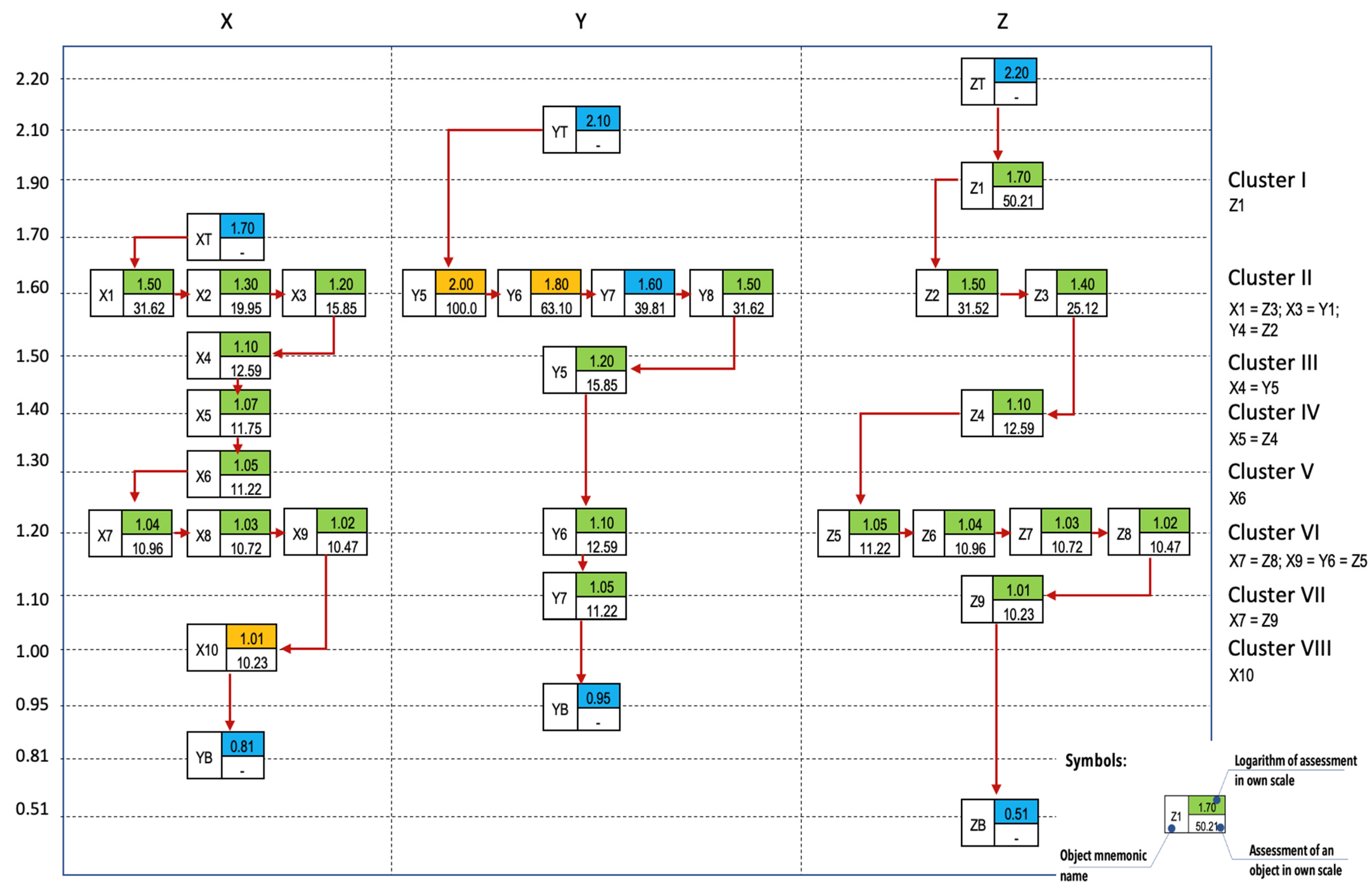
Like group expertise, in which matrix inconsistency is a rule rather than an exception and which leads to cyclic periodic closures, the presence of a cycle (X1 = Z3) & (Z3 < Z2) & (Z2 = Y4) & (Y4 < Y1) & (Y1 = X3) & (X3 < X1) leads to clusters in the solution due to inconsistency of the original matrices. Scales are inconsistent if there is almost no ordered set of their elements. All objects on all private scales are a partially ordered set. In the previous Example 5.1, clusters were formed before a full merger due to the uniformity of risks.
The meaning of the procedure for combining different types of objects into one list in the present example is the synthesis of the integral risk for each object, taking into account its own significance. We are looking for a solution that leads to minimal formation of clusters (mergers of objects) on the general scale. Optimal clustering is essentially the optimal risk of the entire design given the actual material.
The organization of the procedure for assigning an assessment to experts is an independent task. Experts are not required to know either the order of the types that are selected for examination or the values of intra-system indices. It is beneficial to know the results of object comparisons given by other experts. The initial data are a list of “approximate equations” (fuzzy equivalences) compiled by experts. It does not matter that there are no compared objects, and some objects can be present several times. A balanced solution is shown inFigure 6.
Eight clusters were formed, but only two had the same types of objects. This suggests that persistence was partially violated in them, which may indicate a “lie detection” [
35]:
6. Conclusions
This article analyzed the foundations of the future methodology for synthesizing the risk of functional smart expansive systems, taking into account the need to consider the balance between its constituent subsystems: production, development potential and regulation. We propose considering risks as “development anti-potentials” that slow down the reproduction speeds of the entire system. The concept of the geometric integral “anti-risk” is introduced, resulting from the concept of “difficulties in achieving the goal”. Thus, the conceptual definition of risk as the influence of uncertainties on the achievement of the goal of smart expansive systems is formalized.
To assess private risk factors included in the integral risk, we propose a method of vector compression. The idea to build compatible reference solutions, which form the basis for the developed method, represents an alternative to pairwise comparison in the method of analysis of hierarchies and the method of analytical networks.
Further to this, we propose an approach to processing partial matrices of pairwise comparisons, which makes it possible to minimize the disadvantages of the existing methods for working with similar matrices, especially for matrices of large dimensions. The principles of handling pairwise comparison matrices by describing their upper and lower boundaries have been investigated. The developed vector compression algorithm allows us to obtain the weights of compared objects on the basis of matrices of pairwise comparisons containing omissions, without fully restoring the matrix of pairwise comparisons, and also allows us to obtain the weights of given upper and lower boundaries through comparative assessment of pairs of objects.
This paper is not a standalone work capable of covering all issues and presenting the variety of smart expansive systems. These will undoubtedly be the topics of further research. To give an example of where future studies may take us, the smart expansive system in this paper was considered in a linear approximation and stationary case. Beyond the scope of the article, a question must also be raised about the behavior of an intelligent expansive system in a “non-stationary state”, where oscillatory processes (and maybe chaos) may occur. Moreover, the uniqueness of the approximation we chose has not been proven, and the option of using the vector compression method for upper and lower bounds in cases of restrictions imposed on the coefficient (greater than/less than zero) for fuzzy definition of the original matrices has not been considered. We plan to investigate all these and many other avenues in the future.
The proposed method could become an important element in the algorithmic provision of expert advising systems to support decision-making on the management of smart expansive systems, provided there is an appropriately organized procedure for selecting experts to be involved in the assessment of solutions.


