Comparative Analysis of Image Classification Models for Norwegian Sign Language Recognition

Abstract

Communication is integral to every human’s life, allowing individuals to express themselves and understand each other. This process can be challenging for the hearing-impaired population, who rely on sign language for communication due to the limited number of individuals proficient in sign language. Image classification models can be used to create assistive systems to address this communication barrier. This paper conducts a comprehensive literature review and experiments to find the state of the art in sign language recognition. It identifies a lack of research in Norwegian Sign Language (NSL). To address this gap, we created a dataset from scratch containing 24,300 images of 27 NSL alphabet signs and performed a comparative analysis of various machine learning models, including the Support Vector Machine (SVM), K-Nearest Neighbor (KNN), and Convolutional Neural Network (CNN) on the dataset. The evaluation of these models was based on accuracy and computational efficiency. Based on these metrics, our findings indicate that SVM and CNN were the most effective models, achieving accuracies of 99.9% with high computational efficiency. Consequently, the research conducted in this report aims to contribute to the field of NSL recognition and serve as a foundation for future studies in this area.

1. Introduction

An integral part of every human’s life is communication. It is the way they express themselves and understand each other. For most humans, communication comes naturally. They use their ears as input and mouths as output. A less fortunate minority of humans cannot use their hearing or voice to communicate. They must rely on sign language to communicate, where visual movements and hand gestures are used.

According to the World Health Organization, 5% of the world (430 million) struggle with hearing loss, which is likely to increase [1]. Seventy million out of those 430 million are completely deaf [2]. For the deaf and hard of hearing, it is often difficult to communicate with most of the population because a minority speaks sign language. This can cause issues in their daily lives that can be tough to deal with. Using machine learning models to create sign language translation models is one way to assist the deaf and hard of hearing [3].

Typically, when humans do not speak the same language, they use a translator to help them understand each other. The same goes for someone who communicates through sign language when trying to understand an individual who uses oral communication. Sign interpreters are a common way to help the deaf and hard of hearing by translating for them [4]. This is an excellent service where individuals can receive aid from professional sign language interpreters in real-time. The issue with such services is availability because there is a lack of interpreters worldwide for this service always to be available [5]. Machine learning classification models can be implemented to complement sign interprets by recognizing sign language to assist the deaf and hard of hearing.

Using machine learning models for sign language recognition is a well-researched topic. However, despite advancements in sign language recognition, there is a lack of research focused on NSL recognition. Therefore, further research is needed to determine the most effective classification model for NSL recognition to assist the deaf and hard of hearing in Norway and build a foundation for future work.

Our paper compares machine learning classification models to determine which approach is most suitable for NSL recognition to address this issue. The research will use a custom-made dataset containing 24,300 images of 27 NSL alphabet performed by two signers using different backgrounds and lightning.

However, it is essential to note some limitations of our study. The dataset includes images from only two signers, which may limit the model’s ability to generalize across a diverse range of signers. Additionally, while our research provides valuable insights into recognizing NSL signs, it does not offer comprehensive guidelines for creating and implementing complete NSL recognition systems. The results obtained in this study should be seen as a foundation for further research and development.

2. Literature Review

Vision-based sign language recognition is a well-researched topic involving developing machine learning models to recognize sign language. These models use various inputs, such as cameras or sensors, to identify and interpret sign language [6]. There are several categories within sign language recognition, including fingerspelling, isolated words, lexicons of words, and continuous signs [7].

Despite the promising potential of this technology, there is a noticeable gap in research focusing on NSL recognition. This is surprising, considering an estimated 250,000 to 300,000 hearing-impaired individuals in Norway, with 3500 to 4000 being completely deaf [8].

We aim to research specific machine learning models, examining their strengths and weaknesses. We aim to highlight why these models are suitable in our comparative analysis of NSL recognition. We also reference results from previous research papers to provide context and results from research on other sign languages.

2.1. K-Nearest Neighbor

K-Nearest Neighbor (K-NN) is a simple yet fundamental non-parametric supervised classification model requiring little data distribution knowledge [9]. It is known as a lazy learner because there are no parameters for KNN [10]. The general steps to how the K-NN model works written by [11] goes as follows: Based on the input data, KNN finds the K most similar instances to an unseen observation by calculating the distance between them. Then, the algorithm picks the k points based on the training set closest to the new observations made and calls it set A. The last step is assigning the new observations to the most probability class. This is determined by searching for the match that closely looks like the new example among the learned training observations. Because KNN offers such simplicity, it is a commonly used classification algorithm, but when the dataset and its features are large, the model can lose much of its efficiency [12].

Because KNN is a classifier that employs the scikit-learn library in Python, the optimal hyperparameters for the model can be determined using GridSearchCV or RandomizedSearchCV methods. These methods explore all possible parameter combinations and samples from parameter distributions and can leverage cross-validation schemes and score functions provided by scikit-learn [13].

In [14], they created an ISL recognition system where the input image was first categorized as either a single-handed or two-handed sign language gesture using a HOG-SVM classifier. Then, they used feature extraction using SIFT and HOG, and finally, they used KNN to classify the images. They used a dataset containing 520 images to train their model and 260 images to test their model, where 60 of those images were from 6 single-handed sign language gestures and 200 images were divided into 20 double-handed sign language gestures. They achieved an accuracy of 98.33% on their single-handed data and 89.5% on their double-handed data.

In [11], they created a KNN ASL sign language recognition model where they used logarithmic plot transformation and histogram equalization for image reprocessing, then canny edges and L*a*b color space for segmentation. They used HOG for feature extraction on a dataset containing 26 alphabet signs, with 14 samples for training and eight for testing. Their KNN model achieved 94.23% accuracy on their test set.

2.2. Convolutional Neural Network

Convolutional Neural Network (CNN), inspired by the organization of the visual cortex in the human brain, is a popular, supervised machine learning model for image classification tasks due to its ability to generalize well and handle large-scale datasets [15]. CNN models generally consist of convolutional, pooling, and fully connected layers and are trained using backpropagation to recognize visual patterns from the pixels of images [16]. The process is as follows in [6]. First, the convolutional layer extracts the input data by a convolution operation, reduces feature dimensionality through a pooling layer, then passes the most significant features to the fully connected layer to categorize the images.

When creating CNN models, the creator has many options, and the hyper-parameters one chooses will significantly impact the model’s accuracy [15]. A large dataset is crucial for training an effective deep learning model such as a CNN [17]. Dropout is also often an added technique used in CNN models to prevent overfitting. Randomly dropping out neurons during training with a specified probability makes the model more robust and generalized, reducing reliance on any single neuron [18].

In [19], they used CNN for their real-time ASL recognition model, skin color detection, and convex hull algorithm for segmentation of the hand location. Then resized that hand region to 28 × 28 pixels and converted it to grayscale as part of their feature extraction. They achieved 100% accuracy on their test data and 98.05% on their real-time system. Their model was trained on a static fingerspelling dataset created by [20], which consists of 900 images of 25 hand gestures. Reference [21] created a SLRNet-8 CNN model ASL recognition, which was trained and tested on four different datasets containing a combined size of 154,643 in 38 classes (alphabet, 0–9, delete, nothing, space). They grayscaled the images, performed normalization, and resized them to 64 × 64 pixels. Their model achieved an average accuracy of 99.92% on the mixed dataset. Reference [22] created a CNN model using a public dataset from MNIST to create a better-performing model. They performed augmentation to create a total of 34,627 28 × 28 static images of the alphabet (excluding J, Z). The paper was written to compete with state-of-the-art methodologies and achieved an accuracy of 99.67%, which beat other models such as SVM, DNN, and RNN.

2.3. Support Vector Machine

Support Vector Machine (SVM) is a supervised learning model used for pattern recognition and classification or regression analysis. It works by finding an optimal hyperplane that separates the data classes by maximizing the distance between the margin and the classes, reducing classification errors [6]. SVM is an effective machine learning algorithm for sign language prediction, particularly in high-dimensional spaces and when the number of samples exceeds the number of dimensions [23]. While SVM is excellent at classifying, it requires a lot of computational power if the dataset size is too large. Therefore, it can also have computational issues if implemented in real-time applications [24]. According to [24], having a good training set with quality labels and balanced data is essential to creating a successful SVM model. Such as the KNN classifier, SVM is a classifier that employs the scikit-learn library in Python to build the model. Therefore the optimal hyperparameters for the model can be determined using GridSearchCV or RandomizedSearchCV.

Ref. [25] used SVM to create a static PSL (Pakistan Sign Language) model. They used K-means clustering segmentation to separate the fingers and palm area (foreground) from the background. They then used multiple kernel learning to test which feature extraction method was the most effective. They tried EOH (Edge Orientation Histograms), LBP (Local Binary Patterns), and SURF, and the results showed that HOG combined with linear kernel function achieved the best accuracy of 89.52%. They used a dataset containing 6633 static images of 36 alphabet signs from 6 signers to build this model. In [26], they created an SVM model that performed pre-processing by converting the images to grayscale, normalizing the data, and applying gamma correction. For feature extraction, they used Multilevel-HOG. They performed this on an ISL complex background dataset containing 2600 images of 26 classes in grayscale and an ASL dataset containing 2929 images of 29 classes in grayscale. They achieved 92% accuracy on the ISL complex background dataset and 99.2% accuracy on the ASL dataset.

2.4. Key Findings

The finding in our literature search reveals that sign language recognition is a well-researched topic. Primarily for static sign language recognition models, there was a lot of research on KNN, CNN, and SVM models. Based on our summary in

Table 1. Summary of finding different machine learning models.

References	Segmentation	Feature Extraction	Classification	Dataset	Accuracy
(B. Gupta, Shukla, and Mittal 2016)	NaN	SIFT and HOG	HOG-SVM to categorize images as single or two-handed gestures, then KNN for classification	780 ISL images of 6 one-handed and 20 two-handed alphabets	98.33% for one-handed 89.5% for two-handed
(Mahmud et al. 2018)	Canny edges and L*a*b color space	HOG	KNN	572 ASL images on 26 alphabets	94.23%
(Taskiran, Killioglu, and Kahraman 2018)	Skin color detection and convex hull algorithm	Rezised hand region to 28 × 28 pixels and grayscaled it	CNN	900 ASL images on 25 alphabets	100% on test data 98.05% on real-time system
(Rahman et al. 2019)	NaN	NaN	SLRNet-8 CNN	154,643 ASL images on 38 gestures from four different datasets	99.92%
(Mannan et al. 2022)	NaN	NaN	CNN	34,627 ASL images on 26 alphabets	99.67%
(Shah et al. 2021)	K-means clustering to separate foreground and background	HOG	Linear SVM	6633 PSL images on 36 alphabets from 6 signers	89.52%
				2600 ISL images on 26 grayscale alphabets	92% accuracy on ISL
(Joshi, Singh, and Vig 2020)	NaN	Multilevel-HOG	SVM	with complex background
				2929 ASL images on 29 grayscale alphabets.	99.2% accuracy on ASL

, we can see that the segmentation varied across all three classification models. Still, HOG was very popular for feature extraction across all the models. CNN seems to have a lot of research that does not include segmentation or feature extraction of their datasets. Still, they usually balance that out with quality pre-processing and large datasets, one of the most important aspects of CNN models. The accuracy of all the models is very good, and there is no clear indication of which model best suits sign language recognition.

During our research, we found some gaps in the literature that we hope we can assist. Upon studying the literature, there is no research provided on Norwegian Sign Language. We aim to close this gap by creating SVM, KNN, and CNN models for Norwegian Sign Language recognition. Another gap we identified was that many of the datasets the researchers used to train their models were simple images with non-complex backgrounds. While this will achieve great accuracy for the models, an important aspect of image recognition is to build robust models that can generalize. If the models are trained on simple images, it is tough to see how these can be used in real-life applications. We, therefore, aim to create our NSL model based upon a combination of non-complex and complex images with different lighting and backgrounds to develop models that would generalize well. While this might negatively affect our model’s accuracy, we hope it is better suited for real-life situations to further assist the deaf and hard of hearing in Norway.

3. Methods

This section covers the methodology and implementation to find the most effective classification models for NSL recognition. All tests were performed on our local computer with the specs: RTX 3060ti GPU, AMD Ryzen 7 5700G CPU @ 3.8 GHz, and 16 GB of RAM. Figure 1 displays a summary and visualization of the entire data pipeline that was conducted for our methodology and implementation. We started by using our camera for image capturing. The images are then stored as a dataset. Once completed, the dataset is used for three different classification models using their distinct segmentation and feature extraction methods. Finally, the three classification models predict signs of the unseen test set to evaluate their performance.

3.1. Image Acquisition

To build our NSL (Norwegian sign language) recognition model, we had to acquire a dataset containing images or videos of NSL. During our extensive research, we could not find any public NSL dataset and therefore had to start creating our own from scratch. The first step in creating our NSL dataset was determining which sign language category we wanted to create. Because little to no research has been conducted on NSL recognition, we decided that the best approach would be to create a static fingerspelling dataset of the NSL alphabet. We chose this sign language category because languages are built from the ground up, starting with the alphabet. Therefore, we wanted to create a strong base for further work in NSL recognition by creating a baseline for NSL alphabet recognition.

The signs must be performed and statically read to develop a static fingerspelling sign language model. The Norwegian Sign Language (NSL) includes 29 signs from A to Å. However, the letters Å and H cannot be statically displayed, so they were excluded from our research. Static images can display the other 27 signs, most of them as one-handed, but J, P, Q, U, X, Z, and Ø had to be represented as two-handed as there is no static one-handed version. All information about the NSL alphabet and the drawn images in Figure 2 was gathered from the Norwegian Sign Language Dictionary, www.tegnordbok.no accessed on 11 July 2023, which was developed by Statped (State Special Needs Education Service) on behalf of the Norwegian Directorate for Education and Training [27].

Our dataset contains images captured using a Lenovo Performance FHD Webcam with a resolution of 1920 × 1080. However, because we focused on extracting the hand from the images, we implemented a technique called Range of Interest (ROI) to restrict the area of interest to 256 × 256 pixels. This allowed us to retain the high-definition quality of the webcam while minimizing the amount of noise and background the training algorithm had to deal with. In other words, by using an ROI, we ensured that the training process was optimized for accuracy and efficiency.

The Dataset

For our dataset, we created 900 images for each of the 27 NSL alphabet signs, resulting in 24,300 images. The images of one female and one male were taken to ensure that the model could generalize better. We captured 600 images inside with natural and artificial lighting on a white background. Of those, 300 images were taken by the female and 300 by the male. We also captured 300 more images with a complex background to help the model better handle real-world scenarios. These images were taken by the male participant indoors with various objects in the background.

Table 2. Distribution of the NSL dataset.

Alphabet	Male Complex Background	Male Artificial and Natural Lighting, White Background	Female Artificial and Natural Lighting, White Background	Total
A–Ø (Å and H Excluded)	300	300	300	24,300

shows the distribution of the dataset, and Figure 3 illustrates the different scenarios. We also ensured that the dataset was balanced and that all the classes had the same number of pictures, as this is an essential step in making recognition models that are good at generalizing and aim for a high accuracy [28].

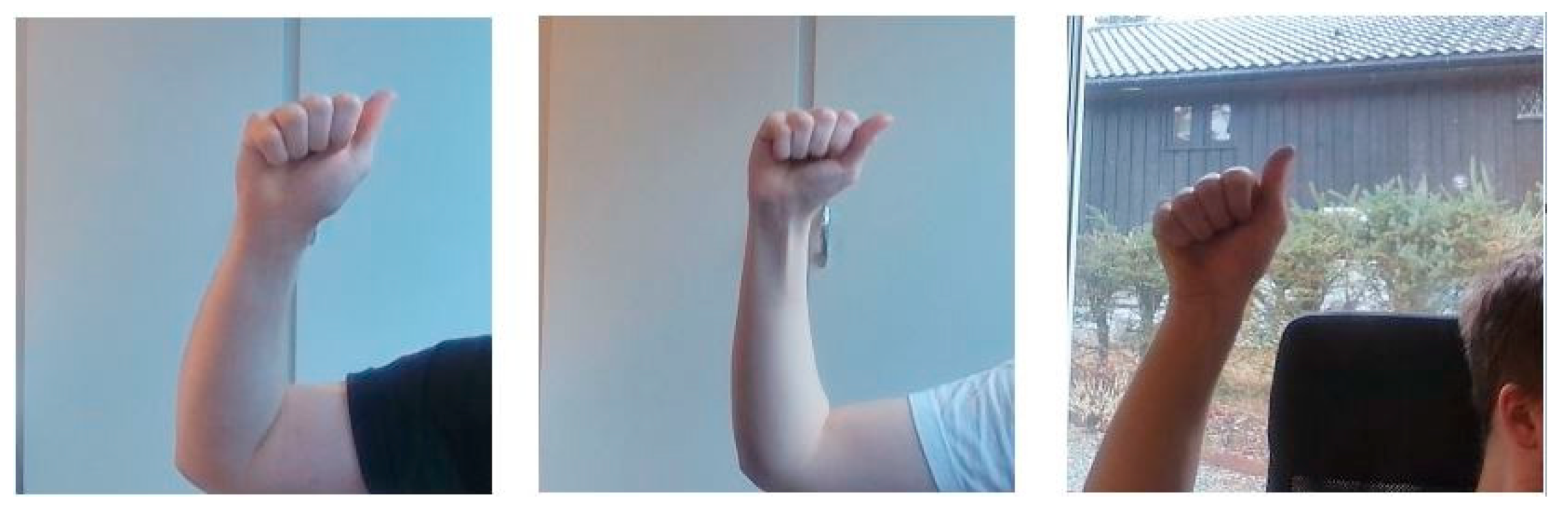
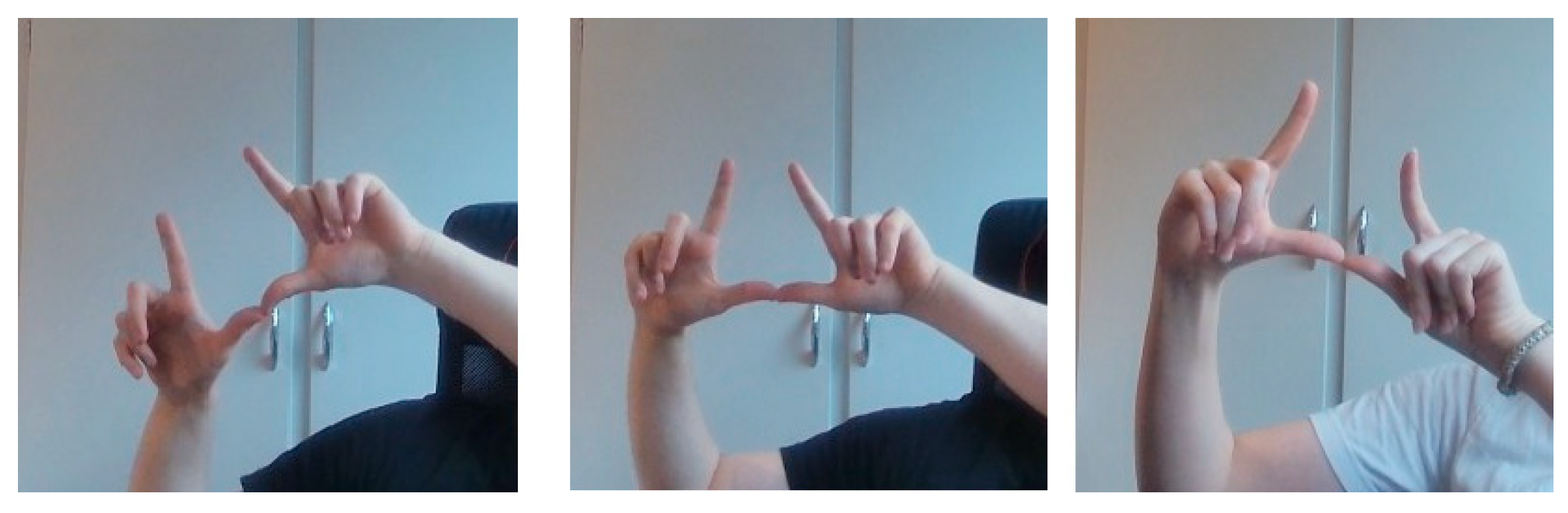
While different backgrounds and people are important steps in creating a dataset for a well-generalized model, we also ensured that the signs we performed during our image acquisition consisted of different angles and rotations of the different signs. In the same way that people pronounce words differently with their voice, signers have different hand orientations when they perform sign language gestures. By incorporating rotated images in the dataset, we can help the model learn to recognize the gestures regardless of the orientation of the signer’s hands. Examples of signs with different angles are shown in Figure 4, and different rotations are illustrated in Figure 5.

Based on the literature we have gathered on sign language recognition, a dataset consisting of 24,300 images represents a substantial baseline for most machine learning models. It should be noted that specific machine learning models may not optimally perform when trained on excessively large datasets. Hence, we decided not to create a larger dataset, recognizing that various machine learning models have different limitations and requirements. In the case of machine learning models such as CNN, which require a considerable amount of data for effective training, data augmentation techniques can be employed to expand the dataset size as needed.

Based on the size of the dataset and the measures taken during the image acquisition process, we are very confident in the quality and diversity of our dataset for NSL recognition. The dataset includes a variety of lighting conditions, backgrounds, and hand orientations. By capturing images from male and female singers and incorporating different angles and rotations, we sought to enhance the generalizability of the dataset for use across various machine learning models. Overall, our dataset can serve as a strong foundation for our own and future research in NSL recognition.

3.2. KNN Model

After creating the dataset, we decided that the first recognition model to create was KNN. We chose this model because it is a simple yet respected model for classification. Additionally, many sign language recognition research studies have utilized KNN, and we wanted to provide similar research for NSL recognition to compare our results. Due to KNN’s struggle with large datasets, we decided not to perform augmentation and use the dataset as is.

3.2.1. Preparing the Data

The KNN classifier is sensitive to noise and large complex datasets. Therefore, the data preparation process plays a crucial role in ensuring the optimal performance of the model. The process we have implemented consists of three primary steps: pre-processing, segmentation, and feature extraction. These steps are designed to transform the raw image data into a structured and standardized format, which can be efficiently utilized to train and evaluate the KNN model while mitigating the impact of noise and complexity. Figure 6 illustrates the different steps described below.

3.2.2. Pre-Processing

The pre-processing step ensures consistency among the images in the dataset. We achieved this by resizing the images from 256 × 256 pixels to a uniform dimension of 64 × 64 pixels. This guarantees that all images have the same dimensions, which is crucial for comparing and processing the images during the later stages of the process. Additionally, it reduces the computational time of the model. This step is illustrated in Step 1 in Figure 6.

3.2.3. Segmentation

The segmentation process isolates specific regions of interest within the images, reducing noise and allowing for more accurate classification. We achieved this using LAB color space segmentation, which provides a more uniform representation of color differences than the RGB color space. The resized images are first converted to the LAB color space, and the Contrast Limited Adaptive Histogram Equalization (CLAHE) technique is applied to the L channel to enhance the image’s contrast. After that, the images are segmented into skin and non-skin regions based on a predefined color range, focusing on the regions containing skin color and effectively removing irrelevant areas within the images. Illustrated are Steps 2 and 3 in Figure 6.

3.2.4. Feature Extraction

Once the images have been segmented, feature extraction provides the KNN model with the most relevant features. We applied the Canny edge detection technique to the grayscale version of the segmented images to achieve this. Subsequently, the skin color mask is applied to the edge image, further refining the features by focusing on the regions of interest. The HOG features are then computed for the masked edge image, generating a feature vector that effectively captures the essential shape and characteristics of the images. L2 normalization is employed to ensure that the HOG features have the same scale and can be effectively compared across images. Illustrated are Steps 4 and 5 in Figure 6.

3.2.5. Model Training and Hyperparameter Tuning

After performing all these steps on the images, the normalized HOG features are flattened and added to a ‘data’ list. The corresponding labels for the images are added to the ‘labels’ list. Finally, the ‘data’ and ‘labels’ lists are converted to numpy arrays. The ‘data’ array is reshaped, maintaining the number of samples (rows) and arranging the HOG features into a 2D array with the appropriate number of columns. This structured format is crucial to train and evaluate the KNN model.

Having prepared the images and extracted their HOG features, we found the best parameters for the KNN model. We began by dividing the dataset into training and testing sets, using a 30–70% split to ensure that the model’s performance could be evaluated on previously unseen data. Following this, we conducted a randomized search combined with cross-validation to find the optimal hyperparameters for the model.

To carry out this process, we constructed a parameter grid containing various combinations of the number of neighbors (K values ranging from 1 to 100), weights (uniform or distance), and distance metrics (Euclidean, Manhattan, and Minkowski). Using cross-validation, we then instantiated a RandomizedSearchCV object to search for the best hyperparameters. To enhance the search efficiency, we set the number of iterations to 50 and employed 10-fold cross-validation. The search process was further expedited by running it in parallel, utilizing all available CPU cores.

Because KNN is already a high computational time model, we decided to create two identical models, one with a 64 × 64 resized image and one with 32 × 32, to compare computational time and accuracy trade-offs.

3.2.6. Experiment 1: 64 × 64 Images

Figure 7 displays the accuracy for the different values of K and the different metrics. Upon completion of the randomized search and cross-validation process, the optimal hyperparameters for the KNN model with a 64 × 64 resolution were identified as follows: ‘metric’: ‘Manhattan’, ‘n_neighbors’: 4, and ‘weights’: ‘uniform’. By training the KNN model with these parameters, we achieved an outstanding accuracy of 99.9% on the unseen test dataset. This accuracy illustrates the effectiveness of the methods we have implemented in this model.

In

Table 3. Classification report of the 64 × 64 KNN model.

Sign	Precision	Recall	f1-Score	Support	Number of Errors
A	1.00	1.00	1.00	271	0
B	1.00	1.00	1.00	271	0
C	1.00	1.00	1.00	272	0
D	1.00	1.00	1.00	267	0
E	1.00	1.00	1.00	280	0
F	1.00	1.00	1.00	261	0
G	1.00	1.00	1.00	272	0
I	1.00	1.00	1.00	280	0
J	1.00	1.00	1.00	247	0
K	1.00	1.00	1.00	262	0
L	1.00	1.00	1.00	295	0
M	1.00	1.00	1.00	255	0
N	1.00	1.00	1.00	285	0
O	1.00	1.00	1.00	263	0
P	1.00	1.00	1.00	252	0
Q	1.00	1.00	1.00	276	0
R	1.00	1.00	1.00	256	0
S	1.00	1.00	1.00	244	0
T	1.00	1.00	1.00	281	0
U	1.00	1.00	1.00	268	0
V	1.00	1.00	1.00	281	0
W	1.00	1.00	1.00	274	0
X	1.00	1.00	1.00	279	0
Y	1.00	1.00	1.00	271	0
Z	1.00	1.00	1.00	283	1
Æ	1.00	1.00	1.00	256	0
Ø	1.00	1.00	1.00	296	0
Accuracy	1.00	1.00	1.00	7298	1

, we present the performance of the 64 × 64 KNN model. The classification report from sklearn metrics provides a comprehensive view of the precision, recall, F1-score, and support for each sign, as well as the number of errors made by the model.

Precision, which measures the model’s ability to identify positive instances correctly, is at 1.00 for all signs, indicating that the model has a high degree of accuracy when it predicts a sign. Recall, which measures the model’s ability to find all the positive instances, is also at 1.00 for all signs, showing that the model is highly effective at identifying all instances of a sign in the dataset. The F1-score, the harmonic mean of precision and recall, is also at 1.00 for all signs, indicating a balance between precision and recall in the model’s performance.

Despite the model’s high accuracy of 99.99%, it is important to note that it took the model 188 s to make predictions on the unseen data. This trade-off between accuracy and time is a consideration for the practical implementation of the model. However, the overall performance of the model demonstrates its robustness and effectiveness in NSL recognition.

To further confirm the model’s accuracy, we aimed to display correctly and wrongly predicted images. Figure 8 shows randomly selected correctly predicted images, where the actual image is displayed as the original image input, and the predicted image is presented as the image version of the HOG features. Figure 9 displays the wrongly predicted image found in the entire model, highlighting the exceptional overall accuracy achieved by the model.

3.2.7. Experiment 2: 32 × 32 Images

The second part of the KNN model result testing involved resizing the images to 32 × 32 to see if the computational time could be reduced without sacrificing too much accuracy. Because all the steps were the same as in Experiment 1, only the results are summarized here. Firstly, a RandomizedSearchCV was performed on the 32 × 32 images, which resulted in the optimal hyperparameters for the KNN model as ‘metric’: ‘Manhattan’, ‘n_neighbors’: 4, and ‘weights’: ‘distance’, with an accuracy of 97.2%. This model only used 18 s to predict the signs of the unseen test data. The result of the RandomizedSearchCV is shown in Figure 10.

Table 4. Classification report of the 32 × 32 KNN model.

Sign	Precision	Recall	f1-Score	Support	Number of Errors
A	1.00	1.00	1.00	265	0
Æ	0.99	1.00	0.99	273	3
B	0.99	1.00	0.99	270	5
C	0.98	0.98	0.98	264	10
D	0.96	0.95	0.96	276	5
E	0.98	0.97	0.98	247	18
F	0.91	0.98	0.94	278	2
G	0.96	0.97	0.97	255	12
I	0.94	0.98	0.96	293	1
J	0.98	0.99	0.99	270	8
K	0.98	0.97	0.97	265	10
L	0.97	0.91	0.94	278	16
M	0.96	0.97	0.96	287	7
N	0.98	0.95	0.96	267	10
O	0.96	0.96	0.96	259	0
Ø	1.00	1.00	1.00	258	5
P	0.99	0.98	0.99	282	4
Q	0.99	1.00	0.99	269	6
R	0.99	0.99	0.99	258	11
S	0.95	1.00	0.97	263	4
T	0.97	0.98	0.98	299	21
U	0.98	0.99	0.99	247	19
V	0.91	0.95	0.93	266	9
W	0.91	0.84	0.88	269	10
X	0.99	0.99	0.99	283	0
Y	0.99	0.95	0.97	280	1
Z	1.00	0.99	0.99	277	0
Accuracy	0.97	0.97	0.97	7298	159

provides a detailed performance report of the model for each sign. While the model performs well overall, with an accuracy of 97%, certain signs such as W, V, F, and L have shown sub-optimal performance.

Precision varies across signs, with the lowest being 0.92 for the sign ‘V’. This indicates that the model has a slightly lower accuracy when predicting this sign. Recall also varies, with the lowest being 0.88 for the sign ‘W’, indicating that the model has slightly lower completeness when identifying this sign. The F1-score is lowest for the sign ‘W’ at 0.90, indicating a slight imbalance between precision and recall for this sign.

The confusion matrix in Figure 11 provides further insights into errors, showing that ‘W’ was wrongly predicted as ‘V’ 18 times, ‘V’ was predicted as ‘W’ 9 times, ‘L’ was wrongly predicted as ‘F’ 7 times, and ‘Y’ was wrongly predicted as ‘I’ 6 times.

Despite these errors, the model’s overall performance demonstrates its effectiveness, highlighting areas for improvement.

3.3. CNN Model

CNNs are known for their ability to handle noise and perform well on image data, so we opted to create the model without employing any segmentation or feature extraction. This is also the approach most of the CNN literature we came across took, such as [21,22].

We chose TensorFlow as the framework for developing our CNN model due to its support for GPU acceleration, enabling faster training. TensorFlow is an open-source platform for large-scale machine learning, which we utilized for importing, pre-processing, splitting, training, evaluating, visualizing, and testing our dataset [29].

3.3.1. Preparing the Data

Although we decided against segmentation or feature extraction, data preparation remains essential for achieving optimal performance with CNN models. We used TensorFlow’s image_dataset_from_directory function to load and pre-process the dataset. The images were resized to 64 × 64 pixels, and the pixel values were normalized to a range of 0–1. We shuffled the data during loading to avoid any biases during training and set a batch size of 32. Once the dataset was prepared, we divided the data into training 70%, validation 15%, and testing 15% sets.

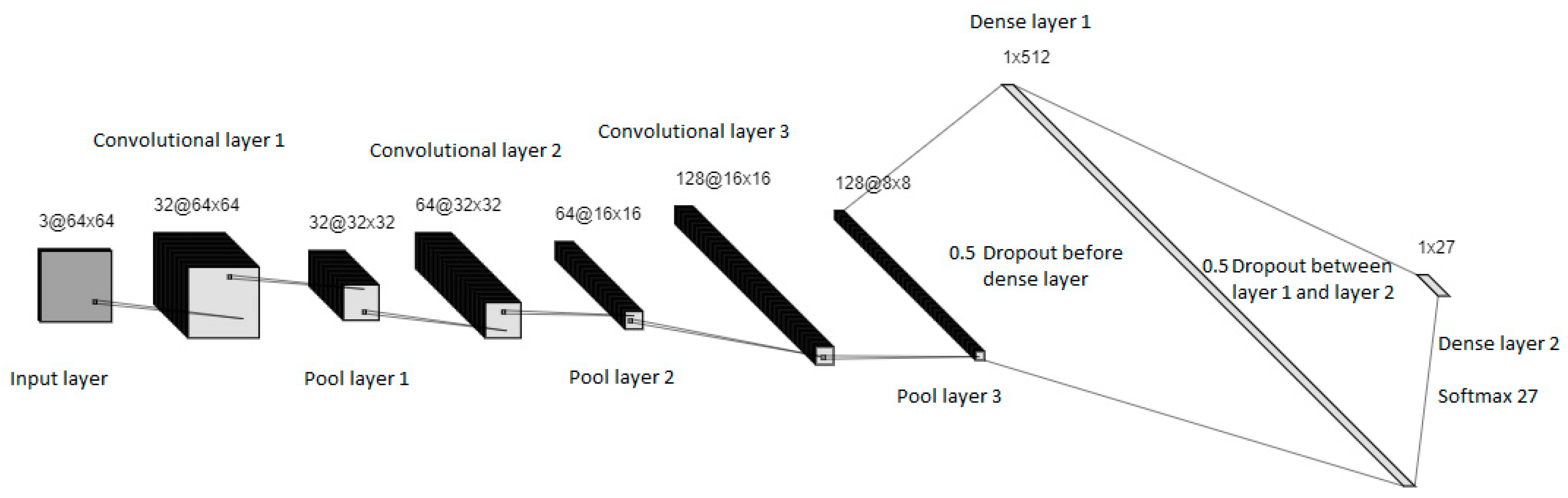
3.3.2. Building the Model

Figure 12 shows the architecture of our CNN model. The CNN model consists of three convolutional layers, each followed by a max pooling layer. The model is then flattened to a 1D array, which is used for the connected layer consisting of two dense layers. Before both dense layers, a dropout layer is added to prevent overfitting. For the convolutional layers, we use ReLU because it is a commonly used activation function.

3.3.3. Model Training and Hyperparameters Tuning

Once the model was built, we started finding the best hyperparameters. Using standard procedures in CNN, we compiled the model using the Adam optimizer, as it is a popular choice for its computational efficiency and low memory requirements [30]. We selected a learning rate of 0.0001, which balances convergence speed and accuracy. The sparse categorical cross-entropy loss function was used, as it is appropriate for multi-class classification problems where the target classes are mutually exclusive. To prevent overfitting during training, we employed an early stopping callback with a patience of 3, which halts the training process if there is no improvement in validation loss after three consecutive epochs.

We initially trained the model for up to 50 epochs so the model could train until it no longer improved and used a batch size of 32. We did this to find the optimal number of epochs for our model to create an accurate model without overfitting it to the training data. The image in Figure 13 displays the results of our initial model, displaying training loss versus validation loss and training accuracy versus validation accuracy. As we can see, the model stopped at epoch 10, meaning the validation loss did not improve starting from epoch 7. This makes sense as it seems like the model achieves close to 100% accuracy on the validation data after 5 epochs. A good indication that the model is not overfitting is that the validation error is lower than the training error, and the validation accuracy is higher than the training accuracy. This is because it indicates that the model is performing well on new unseen data. Due to these findings, we decided to go for 7 epochs for our final model.

3.3.4. Results Analysis

After we had found all the best parameters for our model, we no longer had a use for validation data and divided the data into a new 70% (train) and 30% (test) split for optimal testing. After training the model, we tested the model on the unseen test data.

Table 5. Classification report of the CNN model.

Sign	Precision	Recall	F1-Score	Support	Number of Errors
A	1.00	1.00	1.00	271	0
B	1.00	1.00	1.00	281	1
C	1.00	1.00	1.00	247	0
D	1.00	1.00	1.00	292	1
E	1.00	1.00	1.00	287	0
F	1.00	1.00	1.00	256	0
G	1.00	1.00	1.00	252	0
I	1.00	1.00	1.00	276	0
J	1.00	1.00	1.00	270	0
K	1.00	1.00	1.00	282	0
L	0.99	1.00	0.99	257	0
M	1.00	1.00	1.00	283	0
N	1.00	0.99	1.00	262	2
O	0.99	1.00	0.99	295	0
P	1.00	1.00	1.00	271	0
Q	1.00	1.00	1.00	260	0
R	1.00	1.00	1.00	263	0
S	1.00	1.00	1.00	275	0
T	1.00	1.00	1.00	290	0
U	1.00	1.00	1.00	270	0
V	1.00	0.99	0.99	275	3
W	1.00	1.00	1.00	269	1
X	1.00	1.00	1.00	256	0
Y	1.00	1.00	1.00	281	0
Z	1.00	1.00	1.00	250	0
Æ	1.00	1.00	1.00	259	0
Ø	1.00	1.00	1.00	246	0
Accuracy	1.00	1.00	1.00	7276	8

provides a comprehensive performance report of the model for each sign. The precision, recall, and F1-score metrics, all at 99.9%, illustrate the effectiveness of the model. However, a few signs such as ‘V’, ‘N’, and ‘W’ have shown minor errors.

Precision is at 1.00 for almost all signs, with a slight dip to 0.99 for ‘V’. This suggests a marginally lower accuracy when predicting this sign. Recall also maintains a high score of 1.00 for most signs, with a minor decrease to 0.99 for ‘N’ and ‘W’, indicating slightly lower completeness when identifying these signs. The F1-score is at 1.00 for almost all signs, with a slight decrease to 0.99 for ‘V’, ‘N’, and ‘W’, indicating a minor imbalance between precision and recall for these signs. The model had a training time of 22 s, and predictions on the unseen test data took 22 s.

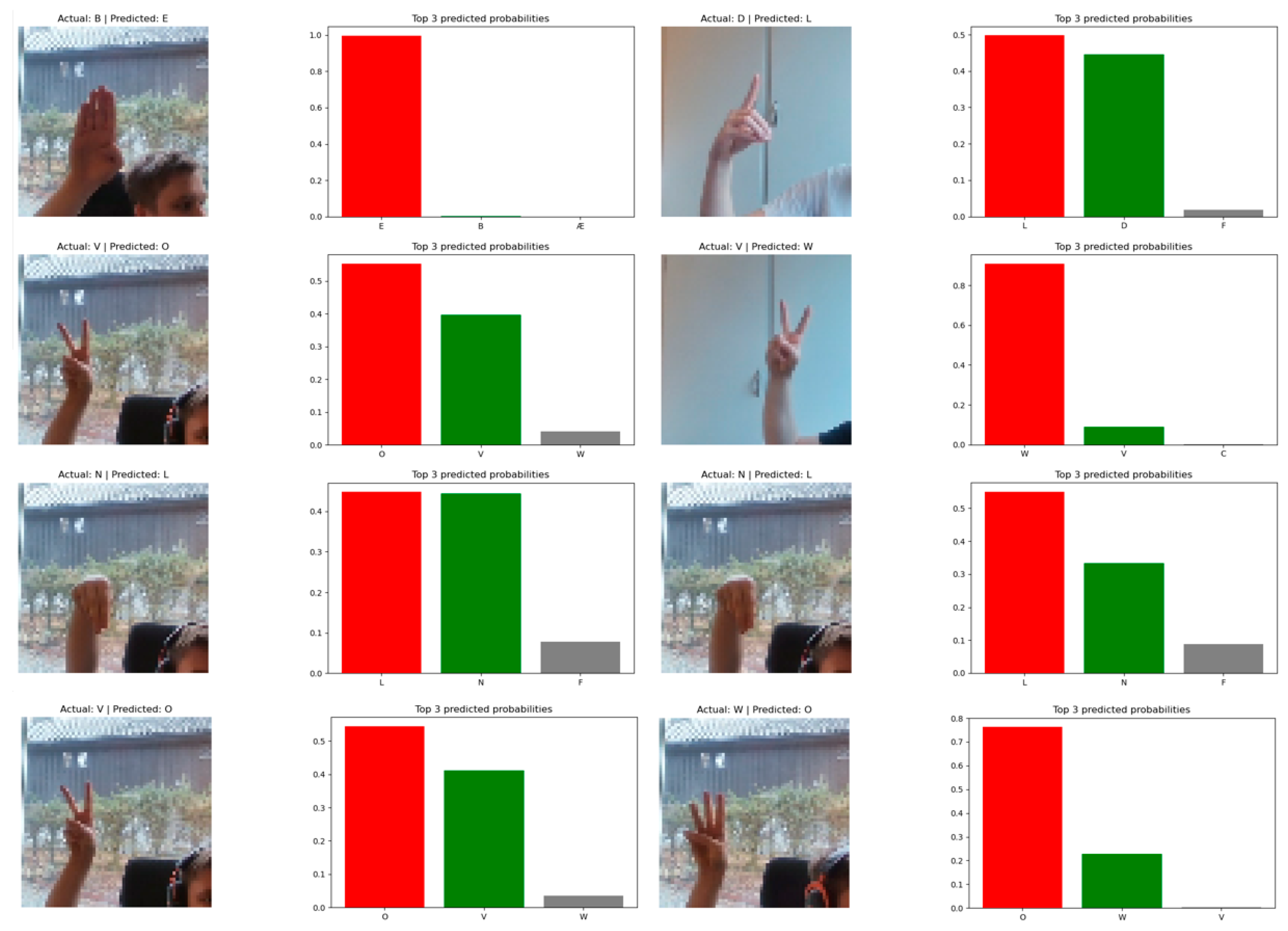
To gain further insight into the wrongly predicted signs, we decided to display the incorrectly predicted images. In Figure 14, we loop through the indices of the incorrectly predicted images and display each image along with its actual and predicted label. It also displays the top three predicted probabilities for the image as a bar chart, with the color of each bar indicating the confidence of the model for different labels, the actual label (green), wrongly predicted label (red), or another label (gray). Looking at the images, we can see that in the two occurrences where the model predicted L but it was N, the model almost achieved the correct answer. While two errors are a very small sample size, and it is hard to say anything conclusive, it could indicate that L and N share some features. The same situation is with V and O, where the model twice predicted that V was O. Again, the model is very close to labeling it correctly, which indicates that although the model predicted wrong, it was still very close to the correct label. Again, because the sample size of wrongly predicted images is so small, we found it hard to conclude anything and decided that these errors were acceptable.

3.4. SVM-Model

The final model we decided to create was an SVM model. This is because it is a powerful and versatile machine learning model that is commonly used in sign language recognition. Because SVM is great at high-dimensional spaces where the number of samples is greater than the number of dimensions, this also makes it a good fit for implementing it in our research towards NSL recognition because the images contain a lot of features.

3.4.1. Data Preparation

The data preparation steps for our SVM model are very similar to that of the KNN model. The reason for this is twofold, it is not a deep learning model such as CNN, and we, therefore, want to train the model on the most important features. Most of the literature we came across, such as [25,26], used feature extraction, segmentation, or both as part of their data preparation. Such as the other models we have created, the pre-processing of the images was to resize them to a fixed size of 64 × 64 for consistency and computational efficiency. Figure 15 illustrates the data preparation steps for our SVM model.

3.4.2. Segmentation

A lot of consideration was given when it came to the image segmentation approach for our SVM model. Our initial thought was to use the same approach we had performed in our KNN model because the LAB color spacing and skin color segmentation we performed for our KNN model were very effective. We did, however, conclude that choosing a different approach for our SVM model would serve greater research value in the field of NSL recognition and decided to choose a different approach.

Such as the segmentation performed in our KNN model, we used LAB color spacing, but instead of segmenting the image based on skin color, we decided to segment the image by separating the foreground from the background. While there are similarities in the approaches, the intent and execution are different.

3.4.3. Feature Extraction

For feature extraction, we decided to go with HOG features as this is a commonly used feature extraction for SVM models. We also found earlier that we had success with HOG for our KNN model. We, therefore, wanted to replicate it for our SVM model without edge detection. In combination with our new approach to segmentation, we concluded that this would lead to valuable research in NSL recognition research.

3.4.4. Model Training and Hyperparameter Tuning

After preparing the dataset and extracting the HOG features, the next step of our process was to proceed with training the SVM model and fine-tuning its hyperparameters. We started by dividing the dataset into training and testing sets, using a 30–70% split to ensure that the model’s performance could be evaluated on unseen data. Following this, we conducted a randomized search combined with cross-validation to find the optimal hyperparameters for the model.

To carry out this process, we first created separate parameter grids for each kernel type: linear, radial basis function (RBF), polynomial, and sigmoid. The grids contained various combinations of hyperparameters specific to each kernel, such as regularization parameters ‘C’, gamma, degree, and coef0. Next, we instantiated RandomizedSearchCV objects for each kernel type to search for the best hyperparameters, utilizing cross-validation. To enhance the search efficiency, we set the number of iterations to 25 for each of the four kernels (total of 100) and employed 5-fold cross-validation. The search process was further expedited by running it in parallel, utilizing all available CPU cores.

Once the randomized search was complete, we extracted the top three models for each kernel type based on their mean cross-validation accuracy. This gave us a total of 12 models to compare. To evaluate the performance of these models on previously unseen data, we trained each of them using the optimal hyperparameters found during the randomized search and tested their accuracy on the validation set.

To visualize and compare the performance of these models, we created a bar plot displaying the accuracy of each model compared with their training time. This allowed us to identify the best-performing and most effective models across different kernel types.

Such as with our KNN model, we decided to conduct two experiments for our SVM model, one with images resized to 64 × 64 and one SVM model resized to 32 × 32.

3.4.5. Experiment 1: 64 × 64 Images

The result of the performance from the top three models for each kernel is displayed in Figure 16. All the models managed to obtain above 99% accuracy. Because there was very little difference in accuracy for the different models, we decided to calculate which model had the best accuracy compared to training time. This was calculated by dividing the accuracy of each model and then their training time to find the optimal model. By considering both accuracy and training time, we found that the kernel that strikes the best balance between performance and computational efficiency is the linear kernel with a C value of 1. This kernel, along with the corresponding hyperparameters, was chosen as the final SVM model for our application.

Using these hyperparameters for our SVM model, we split the data into a 70/30 split and trained the model with a linear kernel with a C value of 1. The result of the model on the unseen data is an incredible accuracy of 99.9%.

Table 6. Classification report of the 64 × 64 SVM mode.

Sign	Precision	Recall	f1-Score	Support	Number of Errors
A	1.00	1.00	1.00	280	0
B	1.00	1.00	1.00	270	0
C	1.00	1.00	1.00	284	0
D	1.00	1.00	1.00	274	1
E	1.00	1.00	1.00	275	0
F	1.00	1.00	1.00	272	0
G	1.00	1.00	1.00	263	0
I	1.00	1.00	1.00	276	0
J	1.00	1.00	1.00	277	0
K	1.00	1.00	1.00	252	0
L	1.00	1.00	1.00	281	1
M	1.00	1.00	1.00	253	0
N	1.00	1.00	1.00	270	0
O	1.00	1.00	1.00	280	0
P	1.00	1.00	1.00	261	0
Q	1.00	1.00	1.00	276	0
R	1.00	1.00	1.00	271	0
S	1.00	1.00	1.00	274	0
T	1.00	1.00	1.00	254	0
U	1.00	1.00	1.00	260	0
V	1.00	0.99	1.00	270	0
W	1.00	1.00	1.00	239	1
X	1.00	1.00	1.00	288	0
Y	1.00	1.00	1.00	260	0
Z	1.00	1.00	1.00	259	0
Æ	1.00	1.00	1.00	271	0
Ø	1.00	1.00	1.00	300	0
Accuracy	1.00	1.00	1.00	7290	3

provides a comprehensive performance report of the Support Vector Machine (SVM) model for each sign. The precision, recall, and F1-score metrics, all at 1.00, offer a detailed understanding of the model’s performance. However, a few signs such as ‘D’, ‘L’, and ‘W’ have shown minor errors.

Precision is at 1.00 for all signs, with a slight dip to 0.99 for ‘V’. This suggests a marginally lower accuracy when predicting this sign. Recall also maintains a high score of 1.00 for most signs, with a minor decrease to 0.99 for ‘V’, indicating slightly lower completeness when identifying this sign. The F1-score is at 1.00 for all signs, indicating a balance between precision and recall for all signs. The training time for this model was 43 s, and the time it took to make predictions on the unseen data was 53 s, indicating a relatively efficient model.

3.4.6. Experiment 2: 32 × 32 Images

Because the data preparation steps in this experiment are the same as in the 64 × 64 one, we will simply provide the results and discuss them later. Figure 17 displays the RandomizedSearchCV for our 32 × 32 model, and the optimal parameters based on training time and accuracy for this dataset is an RBF kernel with a gamma of 0.1 and C value of 100.

Table 7. Classification report of the 32 × 32 SVM mode.

Sign	Precision	Recall	f1-Score	Support	Number of Errors
A	1.00	1.00	1.00	280	0
B	1.00	1.00	1.00	270	0
C	1.00	1.00	1.00	284	0
D	1.00	1.00	1.00	274	0
E	1.00	1.00	1.00	275	1
F	1.00	1.00	1.00	272	0
G	1.00	1.00	1.00	263	0
I	1.00	1.00	1.00	276	1
J	1.00	1.00	1.00	277	0
K	1.00	1.00	1.00	252	0
L	1.00	1.00	1.00	281	0
M	1.00	1.00	1.00	253	0
N	1.00	1.00	1.00	270	1
O	0.99	1.00	1.00	280	1
P	1.00	1.00	1.00	261	0
Q	1.00	1.00	1.00	276	1
R	1.00	1.00	1.00	271	0
S	1.00	1.00	1.00	274	0
T	1.00	1.00	1.00	254	0
U	1.00	1.00	1.00	260	0
V	1.00	0.99	0.99	270	0
W	1.00	1.00	1.00	239	1
X	1.00	1.00	1.00	288	0
Y	1.00	1.00	1.00	260	0
Z	1.00	1.00	1.00	259	0
Æ	1.00	1.00	1.00	271	0
Ø	1.00	1.00	1.00	300	0
Accuracy	1.00	1.00	1.00	7290	6

presents the performance metrics of the 32 × 32 SVM model for each sign. Despite the overall precision, recall, and F1-score metrics being at 1.00, minor errors were observed for signs ‘E’, ‘I’, ‘N’, ‘O’, ‘Q’, and ‘W’. The model’s precision slightly dipped to 0.99 for ‘O’, and recall marginally decreased to 0.99 for ‘V’. The model’s training time was 5.9 s, and the prediction time was 14.9 s, demonstrating its efficiency. With an impressive accuracy of 99.9%, the model’s effectiveness in NSL recognition is evident.

4. Results and Discussion

In this section, we will look at the results of our research, discussing the findings from our comparative analysis to find the most effective machine learning models for NSL recognition. All the models are evaluated based on accuracy, training time, and prediction time shown in

Table 8. Model comparison of all the created models.

Model	Pre-Processing	Segmentation	Feature Extraction	Accuracy	Training Time	Prediction Time
KNN	64 × 64, Normalization	LAB Color Space & CLAHE, Skin Color detection	HOG, Edge Detection	99.9%	0	188 s
KNN	32 × 32, Normalization	LAB Color Space & CLAHE, Skin Color detection	HOG, Edge Detection	97.2%	0	18 s
SVM	64 × 64, Normalization	Foreground/Background detection using LAB Color space	HOG	99.9%	43 s	53 s
SVM	32 × 32, Normalization	Foreground/Background detection using LAB Color space	HOG	99.9%	6 s	18 s
CNN	64 × 64, Normalization	None	None	99.9%	23 s	21 s

. We will also take the time to discuss the different use cases and limitations for each model to offer insight into their suitability for NSL recognition. For consistency in our comparative analysis, all the models were evaluated on the same dataset size with a training and test split of 70/30%.

4.1. KNN Model

Accuracy-wise, the KNN model performs well on our self-made dataset achieving results of 99.9% on the 64 × 64 images and 97.2% on the 32 × 32 images. The results also show the effectiveness of the pre-processing, segmentation, and feature extraction performed on the dataset. However, the results in the table illustrate some of the problems of the KNN classification model, as the model that used the 64 × 64 images took 188 s to make predictions on the unseen test set. When we resized the images to 32 × 32, the prediction time significantly decreased to only 18 s, 1/10th of the one trained on 64 × 64 images. These findings align with the general literature of sign language recognition, as KNN quickly loses its efficiency when the dataset becomes too big or has many features.

4.2. SVM Model

The SVM classification model also achieves an impressive accuracy of 99.9% for 64 × 64 and 32 × 32 image sizes, unlike the KNN model, which has different accuracies for the two sizes. Looking beyond accuracy, the model using the 64 × 64 resized images has a training time of 43 s and a prediction time of 53 s, whereas the model using the 32 × 32 resized images has a training time of 6 s and a prediction time of 18 s. That means that the 32 × 32 SVM model is significantly faster than the 64 × 64 SVM model, with an 86% faster training time, a 66% faster prediction time, and overall, 75% faster in combined computational time.

4.3. CNN Model

The CNN model we created was the only model we decided against creating a 32 × 32 version. This was because the model performs extremely well on the 64 × 64 resized images both in terms of accuracy and prediction time, matching the time of the 32 × 32 SVM model. A very successful model can scale if the dataset can be expanded further by using more subjects and background scenarios.

4.4. Discussion

Based on the results from all our models, all three models can perform NSL recognition with high accuracy. However, there are various trade-offs regarding computational efficiency for the different models. This impacts how these models could be used in real-life scenarios or for future research.

For the KNN model, it is clearly effective and quick if the dataset is not complex or big. Because it is a very easy-to-implement model, we still believe that it has its use cases in niche situations where scalability is not needed. Another potential issue with the KNN model we have created is that it uses skin color detection for segmentation. This is a potential limitation for this model in real-world scenarios as the dataset currently mainly consists of individuals with white skin color. Therefore, the model could face problems if a person of different skin color would use it or if the lighting was different.

The SVM model struck a great balance between accuracy and computational efficiency, making it a very versatile model for many NSL recognition tasks. We were surprised to see that the model maintained its accuracy even when the images were resized to 32 × 32, displaying its robustness and adaptability. While the foreground/background segmentation we performed on the dataset for the SVM model might be sensitive to lightning and background, our dataset contains images with various backgrounds, and we are therefore confident that this would also work well for real-world scenarios.

The results of the CNN model were really encouraging as it offered a high accuracy while maintaining a low prediction time. Because CNN models only become more effective as they are exposed to more data, this model could be trained further on more images to grow and expand. The fact that CNN does not require any segmentation or feature extraction makes it a very attractive model because we do not have to consider lighting, skin color, or other uncontrollable factors. Due to its robustness against noise would also serve as an optimal model for future researchers/contributors willing to create an even more comprehensive data set.

While all three of the models show great results in terms of accuracy, the SVM and CNN model stands out as the absolute strongest contenders in terms of accuracy and computational efficiency in terms of predicting new unseen data. The findings from our comparative analysis of image classification models for NSL recognition offer valuable insights that contribute to further research in the field, ultimately identifying the most effective classification model for NSL recognition.

An observation regarding the near-perfect accuracy leads to the consideration of making the dataset more challenging. Computational enrichment could be explored in future research for more rigorous testing of the model’s robustness and adaptability, such as adding noise or varying image orientations.

5. Conclusions

A significant portion of the global population struggles with hearing impairments, and image classification models can potentially assist the deaf and hard of hearing by translating sign language. During our research, we explored the state-of-the-art for sign language recognition. While our study found that sign language recognition is well-researched, we identified a significant gap in the literature concerning NSL recognition. To address this gap, we conducted a comparative analysis of various machine learning models to provide further research to determine the most effective classification model for NSL recognition. This research aims to assist in communication capabilities for the deaf and hard of hearing in Norway and hopefully take a step closer to implementing machine learning models to help the deaf and hard of hearing, reducing the communication gap between those who are deaf and hard of hearing and those who are not.

Our literature review revealed several popular machine learning models for sign language recognition. Based on the literature, we chose KNN, CNN, and SVM for our comparative analysis as they represent different paradigms in machine learning and have demonstrated promising results in various applications. Our research aimed to effectively compare these models’ data preparation techniques, accuracy, and computational efficiency when applied to NSL recognition.

We created a dataset specifically for NSL recognition. The dataset consists of 24,300 images covering 27 of the 29 NSL alphabet signs, with varying lighting conditions, backgrounds, and hand orientations performed by both male and female signers. The dataset’s comprehensiveness and diversity make it a valuable resource for future research in NSL recognition. It also provides a strong foundation for developing and testing machine learning models in this field.

The study conducted a detailed comparative analysis of three popular machine learning models: KNN, CNN, and SVM. This analysis provided insights into the strengths and weaknesses of each model for NSL recognition. It also provided valuable insight into the effectiveness of different data preparation techniques, such as pre-processing, segmentation, and feature extraction. This will assist future researchers of NSL recognition, and we see this contribution as a benchmark for future work.

Based on the comparative analysis, the research identified CNN and SVM as the best-performing models for NSL recognition regarding accuracy, efficiency, adaptability, and scalability. This finding provides a foundation for future research to implement, refine, improve, and scale these models for practical applications.

The contribution and findings of this paper serve as an incentive for future research and development of advanced, accessible, and cost-effective solutions for NSL recognition. Our work also emphasizes the need for such recognition systems in Norway to improve communication between the deaf and hard of hearing and the hearing majority, thereby reducing communication barriers and enhancing overall accessibility.