1. Introduction
Currently, agri-food producers require technological tools to increase crop production levels to satisfy the food demand of the population [
1,
2,
3]. Food security must be provided, since the world’s population has a growth rate of approximately 1.09% per year, which demands greater requirements for the agricultural industry to provide increasingly higher yields [
4]. However, agricultural production costs ignore the immediate negative impacts on other users [
5]. In this context, traditional agricultural practices are causing environmental damage, leading to the degradation of natural resources such as soils due to the excessive use of fertilizers and pesticides that the farmer scatters homogeneously to avoid delays in product development [
6,
7]. Precision agriculture (PA), a combination of technology and agronomy, offers a viable solution to the challenges faced by traditional farming practices. PA focuses on the integrated management of plots by using technology tools such as the Internet of Things (IoT), machine learning, and drones to gather data on crops’ growth and health.
PA seeks to identify the variations in the conditions of the plot to carry out differential spatial management. UAVs (unmanned aerial vehicles) have generated tremendous interest in crop monitoring due to the great potential they can offer in the agricultural sector to verify the parameters that affect the development of plants [
8,
9]. Aerial images identify growth scans and areas of crop deterioration [
10]. This technology helps soil conservation and sustainable agriculture, specifies the causes of soil damage, and identifies damage caused in the early stages of cultivation [
11].
PA enables decision-making to improve production through an adequate understanding of the means of agricultural production [
12]. Additionally, the current ability to process images with increasingly faster computers aids in analyzing some features of an object. The use of digital image processing (DPI) helps to solve the problems of image segmentation, object area, and characteristics on image-invariant scales, among others. According to [
13], information can be obtained with the support of UAVs, which can later be used with different IPR techniques to obtain different behavior patterns in a given area. Various techniques, such as thresholding, different transformations of color spaces, normalized difference vegetation indices (NDVIs), and Excess Green Vegetation (ExG), among others, have been implemented to extract characteristics that define the state of crops such as grains and vegetables [
13].
DPI has become an essential tool in precision agriculture. An example of its application is the use of the red–green–blue model (RGB) to carry out Lab color space transformations and the k-means algorithm to extract weeds from onion crops. For example, in [
14], the authors mentioned that RGB space colors offer a very high spatial and temporal resolution. In this work, they performed a biomass monitoring system by processing RGB images obtained by a camera mounted on an unmanned aerial vehicle. They reported a 95% accuracy by implementing image analysis instead of invasive sensors. This application highlights the potential for using advanced technologies in PA. DPI enables farmers to detect crop problems early, allowing for targeted interventions and reducing costs while minimizing the environmental impacts. The application of DPI in precision agriculture has the potential to revolutionize the agricultural sector and ensure sustainable agriculture practices [
15,
16]. Notably, image processing and computer vision applications in the agriculture sector have grown due to reduced equipment costs, increased computational power, and growing interest in non-destructive food-assessment methods [
17].
In recent years, there has been increasing interest in using data analysis and machine learning techniques to identify the patterns affecting crop growth and productivity. The authors of [
18] presented a Mutual Subspace Method as a classifier in different farm fields and orchards, achieving 75.1% accuracy in high-altitude image-acquisition systems. By analyzing large amounts of data, such as weather patterns, soil quality, and crop yields, farmers and researchers can gain insight into the factors that influence crop growth and use this information to improve agricultural practices. Alibabaei et al. estimated tomato yield based on climate data, irrigation amount, and water content in the soil profile as input variables for Recurrent Neural Networks. The results showed that the Bidirectional Long Short-Term Memory model achieved an R
of 0.97 [
19].
The remarkable work provides alternative solutions for crop monitoring and preventing disease factors. However, the conditions of an area with an arid climate can affect the quality and quantity of the food harvest, which makes it a challenge to propose alternatives that can improve and make agricultural processes more efficient without compromising land resources [
20].
In this context, this study focuses on the state of Zacatecas, Mexico, a significant agricultural region known for producing corn, beans, and chili peppers. This study proposes a solution to increase the production percentage and minimize losses by analyzing the patterns that most impact crop growth during its phenological stage.
Crops suffer losses during their development cycle, and it is necessary to increase production each time. Therefore, this work aims to analyze which patterns most affect crop growth during its phenological stage and identify these patterns at an early stage. In this way, a proposed solution to increase the production percentage of the crop is offered, and a determination is made of which patterns most influence crop growth throughout its phenological stage in the state of Zacatecas, Mexico. It was concluded that humidity, cloudy weather, and leaf blight greatly impacted crop development and overall agricultural production. This fungal disease can damage the foliage and ultimately lead to crop loss.
2. Materials and Methods
2.1. Development of Experimentation
Crop development for this work occurs in the municipality of Fresnillo, Zacatecas, Mexico, with Cartesian coordinates 23
06
30.6
N 102
38
26.3
W, as shown on the maps in
Figure 1. A UAV Phantom 4 Pro with an RGB camera, a GPS/GLONASS system, and a 20-megapixel camera 4K resolution flew over onion crops (Allium Cepa) to capture photographs throughout the crop cycle. It presented a flight every week from March to July 2019 for 16 weeks, obtaining an average of 758 images in a land area of approximately three hectares at 20 m in height and a series of 5m. These series verified the optimal height, starting at 2 m and continuing at 5, 10, 15, 20, and successively up to 120 m.
2.2. Data Processing
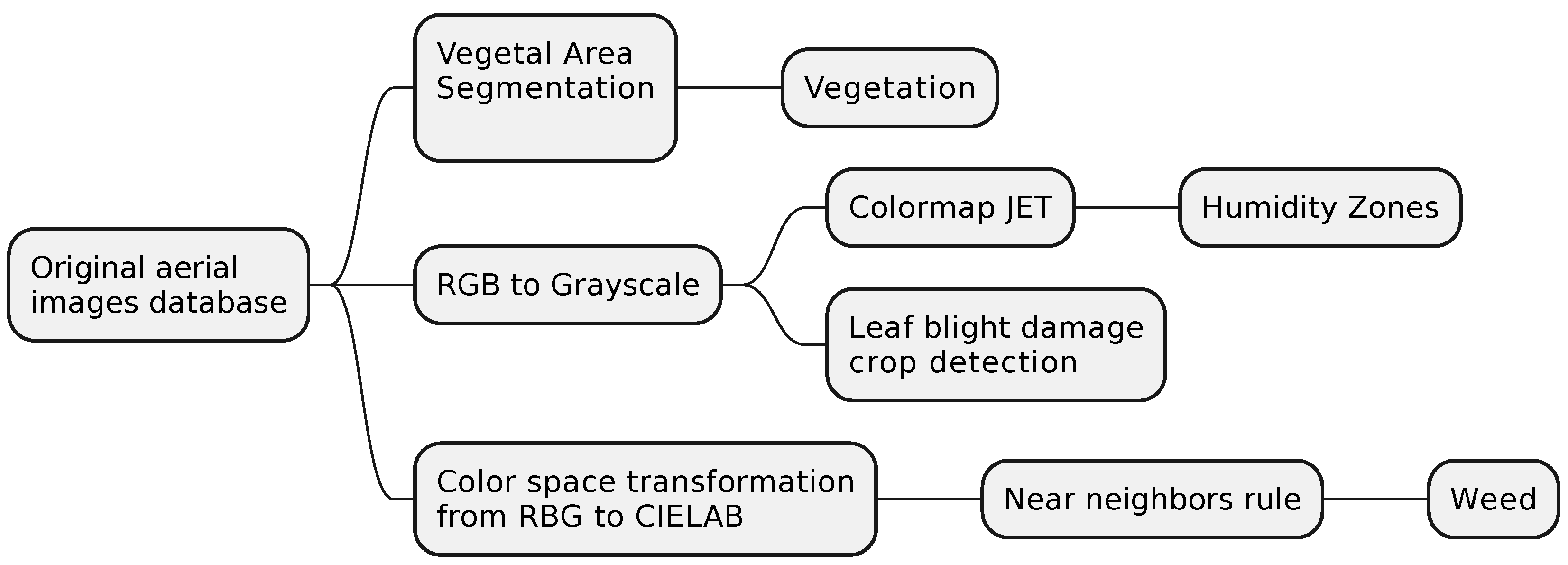
Image processing allows the detection of the vegetal area. Using grayscales allowed spotting damage due to blight, and a transformation to Jet coloration helped recognize wet areas. For weed detection, a color transformation of the RGB-CIELAB plane was made using the algorithm of near neighbors. See
Figure 2.
2.2.1. Vegetal Area Segmentation
In another work, ref. [
21] used a color segmentation technique to obtain and separate green areas in an image by calculating the excess green value ExG, as shown in Equation (
1).
Due to variations in illumination in photographs, an experimental modification without significant luminosity variation was made, described in Equation (
2), as suggested by Tang and Liu [
22], in order to trace a green sphere in a video, looking for a better way to segment the plant area.
The following images compare the segmentation performed using the ExG index and the one proposed under the name
, as determined by Equations (
1) and (
2).
where
r,
g, and
b are red, green, and blue color channels in the RGB space, respectively.
2.2.2. Blight Damage Detection
The grayscale conversion model, described in Mathworks
™ [
23] and indicated by Equation (
3), was applied to RGB images, as mentioned by [
22]. Only the luminescence values were implemented, omitting saturation and hue, obtaining a linear combination of RGB values in a grayscale.
where
R,
G, and
B are the color channels in the RGB space. Grayscale images have 8-bit values from 0 to 255, allowing threshold values for image segmentation.
2.2.3. Humidity Detection
Each pixel in the image grayscale is mapped to the colormap jet (200). Transforming the color to the jet plane generates an RGB image with uninterrupted areas of pure color from a binary image, generating a multicolored image.
2.2.4. Weed Detection
To perform weed detection in the CIELAB, color-space-based segmentation (CIE 1976
L a b) was implemented as a model used to describe all colors the human eye can perceive. It is described in Equation (
4), an international standard for color measurement specified by CIE in 1976 [
24]. This color space consists of an
L brightness layer with a black–white ratio from 0 to 100, with the chromaticity layer
a indicating where the color falls along the green–red axis, with negative values for green and positive for red. The chromaticity layer
b indicates the blue–yellow axis with negative values for blue and positive values for yellow.
The transformation of primary colors is performed and integrated into the XYZ color model, where
X,
Y, and
Z represent vectors in a three-dimensional space of the color described in Equation (
5).
where
R,
G, and
B refer to the red, green, and blue colors of the RGB color model, while
X,
Y, and
Z represent the CIE color set.
f is described by Equation (
6):
and the CIE XYZ are the tristimulus values of the reference white point. For this study, illuminant D65 was used, where
, simulating midday light with a correlated color temperature of 6504 K.
In the color space in this representation,
L represents the luminosity of an object,
a represents the variation from green to red, and
b represents the variation from blue to yellow. With this color transformation, a sample region was selected for each color. The average color of each sample region was calculated in space
ab, using Equation (
4). These samples were used as color markers to classify each pixel in the image. Once the color label was found, the near-neighbors technique was implemented, which is a machine-learning method that classifies an unknown sample according to its neighbors [
25]. Each pixel is classified based on calculating the Euclidean distance between that pixel and each color marker, as indicated by Equation (
7).
where
a and
b are the CIELAB color channels
a and
b while
and
are the values of the markers found for the pixels. The smallest distance denotes the match with a particular color label. The label corresponding to the green color was selected, and the erosion and dilation operations were applied to extract the weed areas.
3. Results
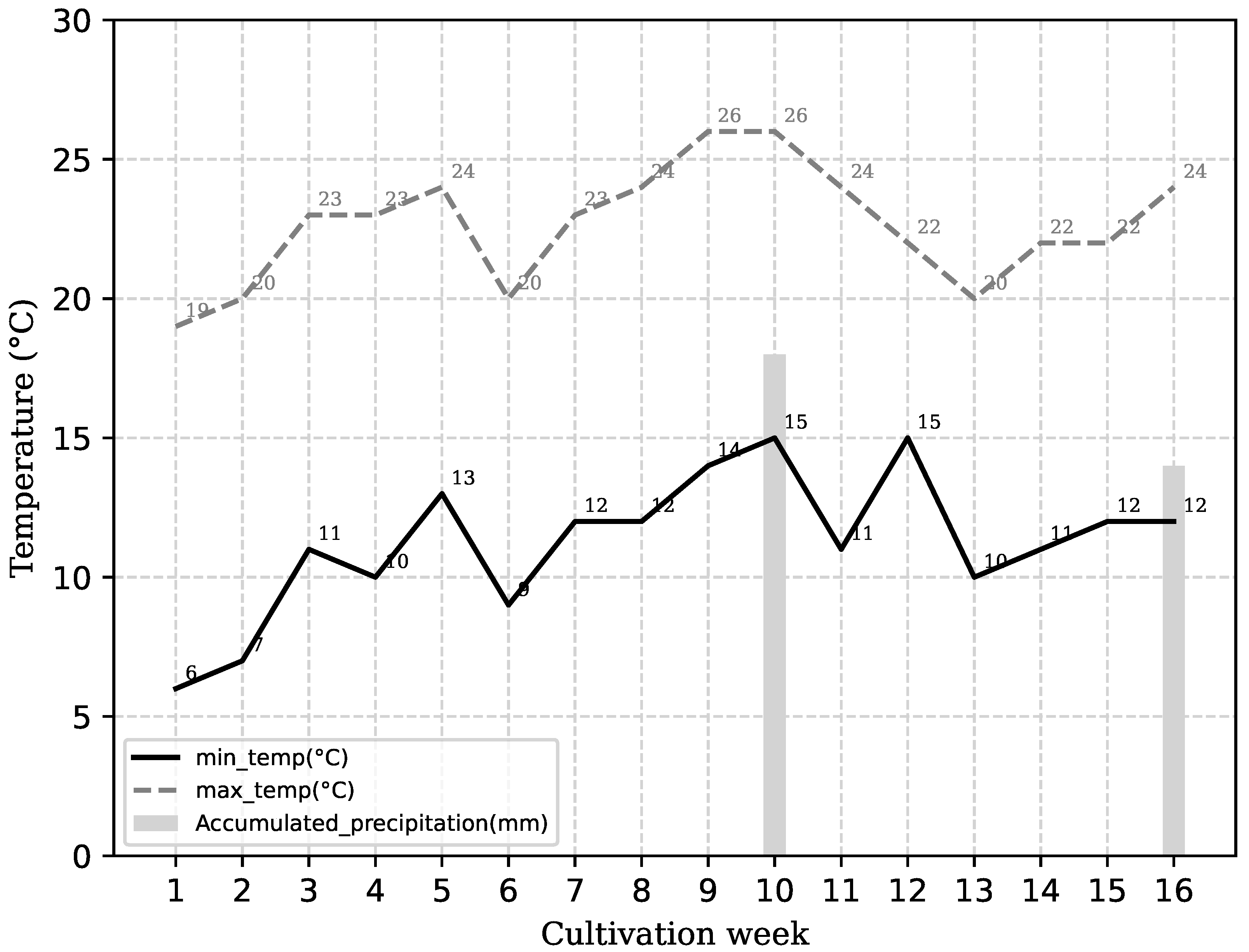
The temperature and rain conditions obtained throughout the phenological cycle are shown in
Figure 3. The minimum temperatures varied between 7
C and 15
C. The maximum temperatures fluctuated between 20
C and 26
C, remaining stable.
Accumulated precipitation was nil for most of the period, except for weeks 10 (18 mm) and 16 (14 mm). Due to low sun conditions, an ideal environment for fungus propagation was generated, causing significant damage. Both graphs were created with data extracted from AccuWeather© [
26].
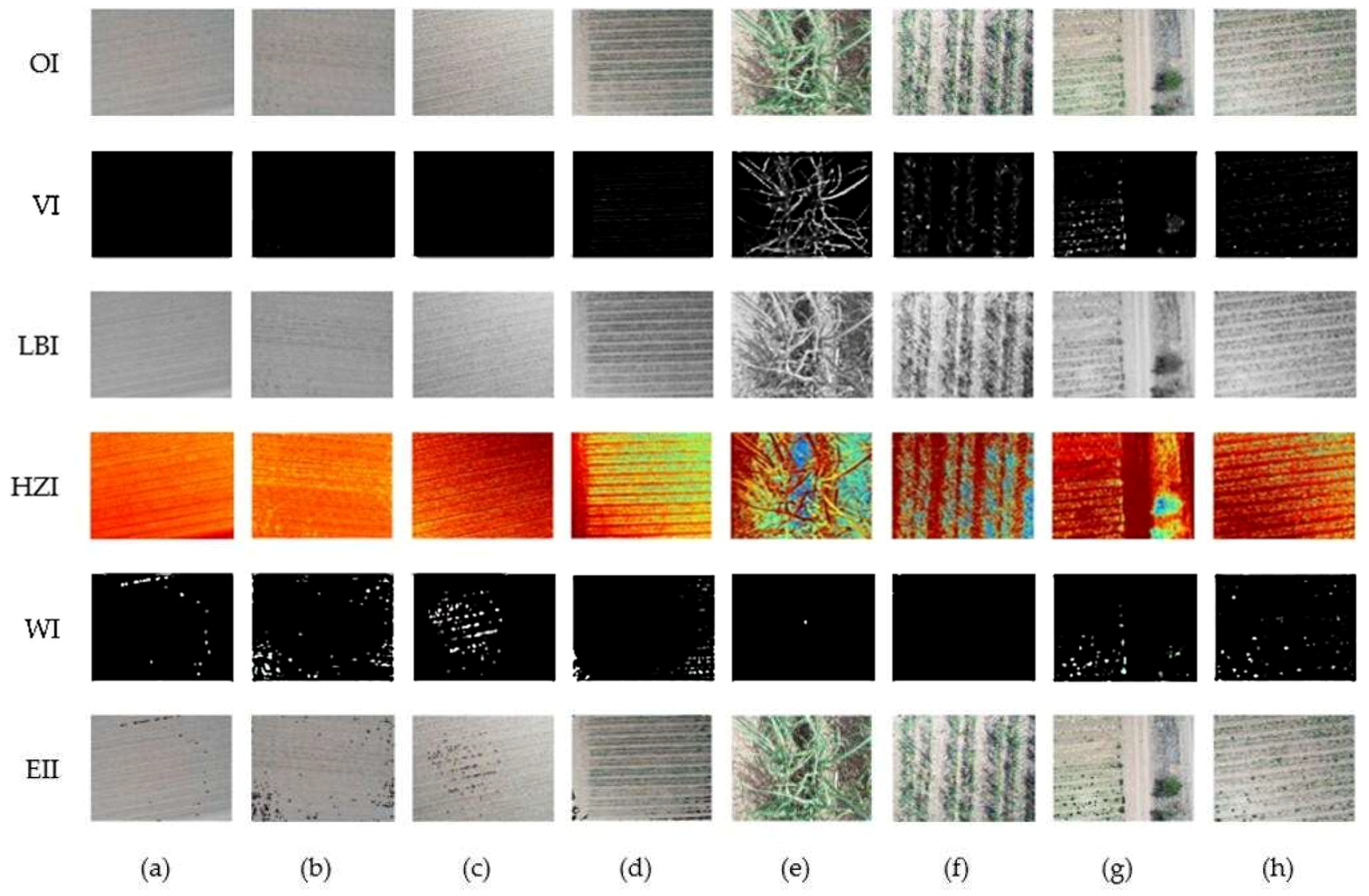
Figure 4 compares the crops’ temporal development and the different processes applied to the selected representative images obtained from the plot, where the Original Image (OI), Vegetation Image (VI), Leaf Blight Image (LBI), Humidity Zones Image (HZI), Weed Images (WI), and Error Identification Images (EII) were analyzed. These terms represent the subtraction of OI and WI when analyzing the error between both.
In this selection, the segmentation of the areas was applied in VI green using Equation (
1), representing vegetation segmentation, including cultivation and weeds.
In LBI, the RGB image is taken from the grayscale image to highlight the damage caused by white leaf blight, while the rest of the image contains grayer tones, making detection at low altitudes easy. At heights greater than 5 m, the damage caused by fungi is not visually detectable enough. HZI is the result of making a Jet-type mapping of the grayscale images, in which the dry areas are highlighted in reddish color while the humid areas are presented lighter colors, in blue passing through yellow.
The RGB to CIELAB transformation was applied to detect weeds using the nearby neighbors’ decision rule and Euclidean distance metric with erosion and dilation. Results were affected by image brightness, with correct results only obtained in certain lighting conditions [
18], such as a cloudy day between 9:30 am to 11:00 am during week 16.
In the first weeks, abrupt changes affecting onion development were undetected. At the same time, it was not possible to detect the crop at heights greater than 20 m. Therefore, there were no significant results in the first four weeks.
On the right side of the images, a sample of the analysis is presented at different heights (2, 5, and 20 m). The ideal height to detect vegetation areas, even with visible damage, was determined to be 5 m. However, the humid areas are visible at 20 m since they do not depend on the height of the plant but on water leaks or excessive irrigation.
3.1. Segmentation of Plant Area
The plant area was segmented using two different indices. First, the ExG index was used. However, this index produced a poor response in photographs with excessive or poor lighting. Therefore, the plant area was also segmented using JustGreen, an experimental index described in Equation (
2). JustGreen provided a more robust response to the amount of illumination, allowing a more accurate estimation of the plant area than the ExG index.
Figure 5 compares the ExG and JustGreen indices.
As shown in
Figure 5b, the plant area is lost in photographs with different lighting. In
Figure 5c, the result of the JustGreen concerning the ExG is more reliable than the original image in
Figure 5a The JustGreen implemented transformation, allowing the vegetation only to be seen, as shown in
Figure 4 VI. This figure presents a sample of the area obtained in Equation (
1) to estimate the vegetation and obtain its segmentation.
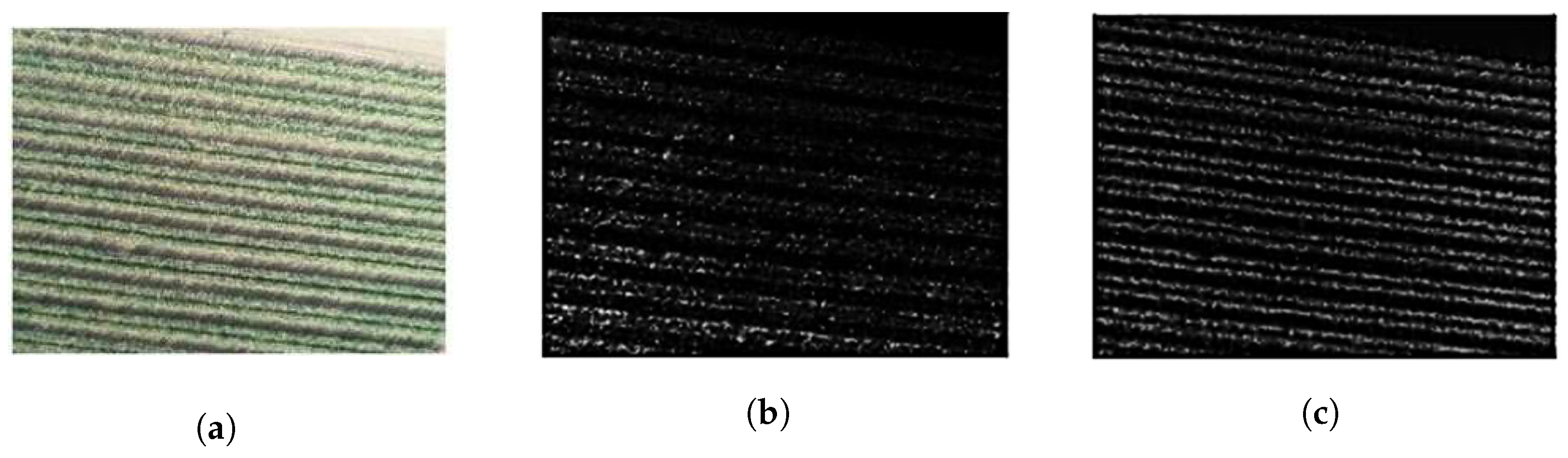
3.2. Leaf Blight Damage
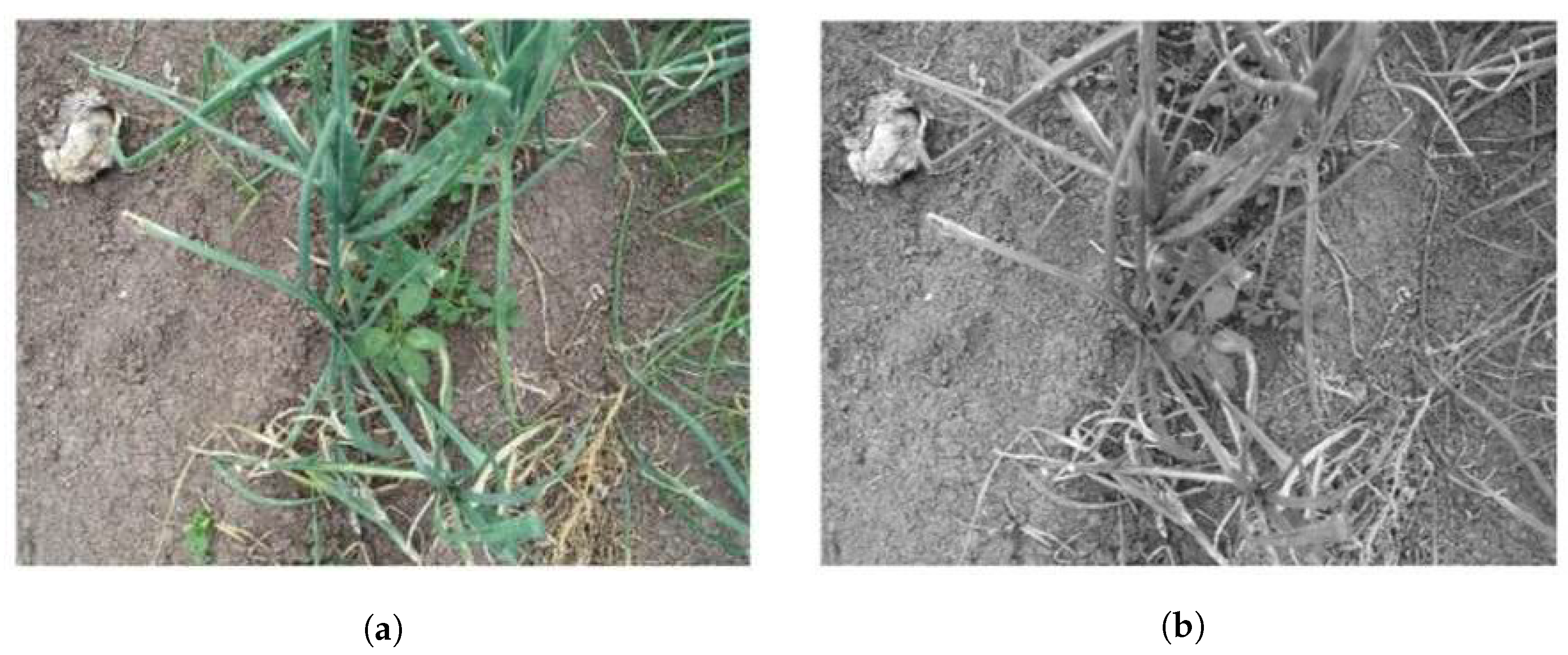
The damage caused by leaf blight can stop the growth of the plant. Hence a gray-scale transformation was applied to highlight the blight damage of the objects in the background to properly present the damage by the fungus.
As shown in
Figure 6a, an adequate inspection is more difficult when objects are near the plant.
Figure 6b further separates the white area generated by the fungus from the rest of the image in darker grays.
The damage is not clearly distinguished at a height greater than 5 m.
3.3. Humidity Detection
When using the gray-scale images towards the jet200 colormap, it was possible to distinguish dry from wet soil, which allowed for detecting areas with excessive humidity and/or waterlogging. The row HZI in
Figure 4 shows the performance of the jet plane in detecting wet areas. The humidity was visible at different heights. The dry soil appeared reddish, while the humid area was shown in light colors close to blue. This mapping is affected by the plant’s shade due to humidity.
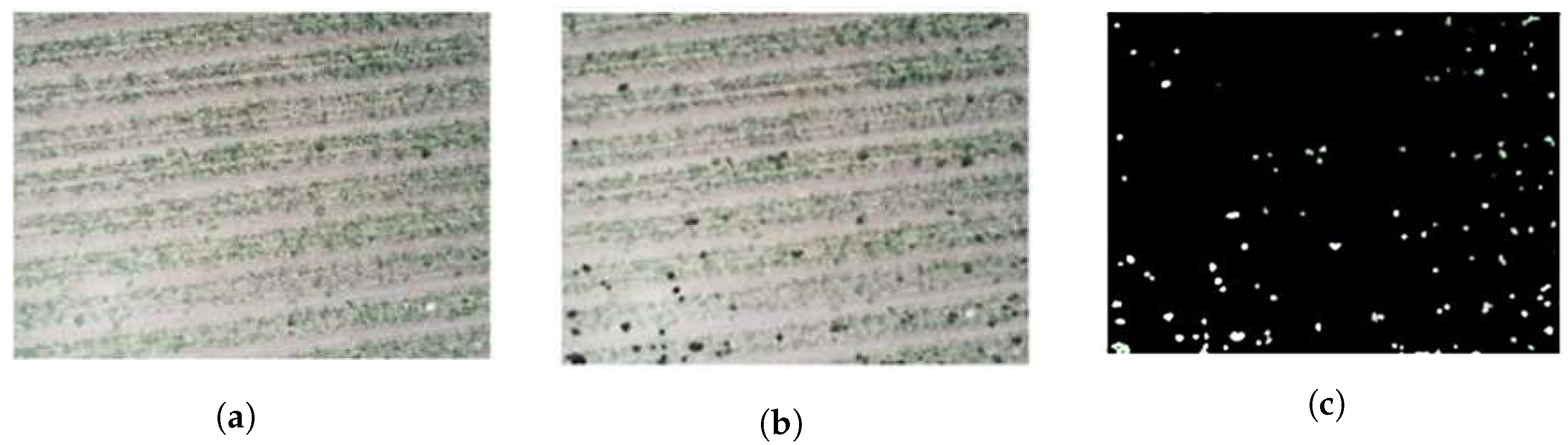
3.4. Detection of Weed
Figure 4 shows that the EII parameter indicates poor results for the decision rule of nearby neighbors, as lighting variations in each set of images affect the algorithm’s ability to detect weeds in most of the data. For the early weeks, it presented many errors, but in the last week, it obtained hits in detection
Figure 5c, with image
Figure 6b showing the error obtained in the algorithm.
Figure 5a is the original image.
Figure 7 shows the area with weeds detected within the crop using the CIELAB transformation, the rule of close neighborhoods, and dilation. The original image at 20 m high is shown in
Figure 7a, as well as the overgrown area detected in
Figure 7b. The detection error is visualized by subtracting the two images in
Figure 7c (overlapping them).
The final production of the crop was 25.00
. In comparison, the agri-food and fisheries information service (SIAP) [
27] reports a general production in Zacatecas of 40.166
in 2019 throughout the agricultural year, in which higher irrigation is presented as temporary in July. This is due to weather conditions and environmental damage.
4. Discussion
In [
28], a threshold must be applied to each plant color, whether healthy or diseased, for example, between the healthy crop and the blight damage that causes different coloration in the plant.
The segmentation using Equation (
1) allowed the plant area to be extracted without using a segmentation threshold.
Using the algebraic transformation of Equation (
1) has the advantage of segmenting the entire plant area with gray colors.
This study [
29] required median filters and Otsu thresholding to detect disease spots, with blight as the cause of discoloration in the crop.
The use of gray scales in the identification of diseased areas results in a low computational cost and, thus, shorter processing time, compared to the processing applied by them, as an alternative to the plant-to-plant detection of diseased areas. To detect humid areas, laboratory analysis of soil samples or the use of instruments that indirectly help to measure humidity or/and temperature is commonly required. However, it is only feasible to place a few sensors since it becomes costly. The proposed method is a non-destructive alternative that estimates the wet area in the entire crop. This allows farmers to focus on areas with prolonged humidity as a possible risk factor for fungal damage or diseases caused by blight. Farmers can take appropriate measures to prevent fungal damage by identifying these areas. The weed detection technique presented the need to manually define the size of the weed, making it a deficiency in non-uniform areas of weed development. However, as seen in
Figure 6, it has good detection at 20 m high, regardless of the lighting in the photograph.
The blight appeared because the temperatures remained stable, averaging 10 to 25 C. This stable temperature range facilitated its development, resulting in the deterioration of the plant’s growth. As a result of the presence of blight, the growth of the plant is deteriorated.
5. Conclusions
Identifying diseased areas using grayscale images is an effective and low-cost approach to the detection of plant disease. Moreover, the results demonstrated a simplified representation of the plant tissue, which can help to reduce the computational cost of image-processing techniques. This method also provides a non-destructive alternative for estimating wet areas in the crop, allowing farmers to focus on areas with prolonged humidity and prevent fungal damage or diseases by blight. However, the weed-detection technique presented some limitations in non-uniform areas of weed development. The blight appeared due to stable temperatures that facilitated its development, resulting in the deterioration of the plant’s growth. Overall, this study highlights the potential of digital image-processing techniques in improving crop management and identifying areas for targeted intervention, ultimately contributing to more sustainable and productive agricultural practices.
Monitoring the onion crop allowed us to identify parameters that affect its development, such as weeds, water leaks, excess humidity, vegetation deficit, and a crucial parameter known as blight.
Blight developed due to the lack of constant irrigation in adequate amounts, resulting in approximately 16 mm of precipitation received in the tenth weekend. During this period, the presence of a fungus due to the cloudy climate and low sunlight significantly affected the last weeks of crop development.
In addition, the irrigation deficit resulted in a lower yield than in the state of Zacatecas, where only 50% of medium-sized onions were produced. Approximately 20% of the production was lost due to the blight and on-site irrigation conditions.
To control the blight problem in this variety, it is recommended to irrigate the crops adequately and not to expose them to water stress. However, over-watering should also be avoided since excessive humidity in the soil and high temperatures create ideal conditions for fungi and weed development.
Author Contributions
Conceptualization, D.D.-C. and J.R.-R.; Methodology, G.D.-F. and J.M.Á.-A.; Software, D.D.-C.; Validation, D.D.-C. and G.D.-F.; Formal analysis, J.R-R.; Investigation, D.D.-C.; Resources, J.R.-R. and G.D.-F.; Data curation, D.D.-C. and J.R.-R.; Writing original draft preparation, review, and editing, C.A.O.-O., J.R.-R. and G.D.-F. All authors have read and agreed to the published version of the manuscript.
Funding
This research received no external funding.
Institutional Review Board Statement
Not applicable.
Informed Consent Statement
Not applicable.
Data Availability Statement
Not applicable.
Acknowledgments
The authors thank CONACYT for funding this work and Ruben García for the edition of the manuscript.
Conflicts of Interest
The authors declare no conflict of interest.
References
- Bakthavatchalam, K.; Karthik, B.; Thiruvengadam, V.; Muthal, S.; Jose, D.; Kotecha, K.; Varadarajan, V. IoT Framework for Measurement and Precision Agriculture: Predicting the Crop Using Machine Learning Algorithms. Technologies 2022, 10, 13. [Google Scholar] [CrossRef]
- Tatas, K.; Al-Zoubi, A.; Christofides, N.; Zannettis, C.; Chrysostomou, M.; Panteli, S.; Antoniou, A. Reliable IoT-Based Monitoring and Control of Hydroponic Systems. Technologies 2022, 10, 26. [Google Scholar] [CrossRef]
- Sanida, M.V.; Sanida, T.; Sideris, A.; Dasygenis, M. An Efficient Hybrid CNN Classification Model for Tomato Crop Disease. Technologies 2023, 11, 10. [Google Scholar] [CrossRef]
- Mirás-Avalos, J.M.; Rubio-Asensio, J.S.; Ramírez-Cuesta, J.M.; Maestre-Valero, J.F.; Intrigliolo, D.S. Irrigation-Advisor—A Decision Support System for Irrigation of Vegetable Crops. Water 2019, 11, 2245. [Google Scholar] [CrossRef]
- Padilla-Bernal, L.E.; Reyes-Rivas, E.; Pérez-Veyna, Ó. Evaluación de un cluster bajo agricultura protegida en México. Contaduría Adm. 2012, 57, 219–237. [Google Scholar] [CrossRef]
- Ferentinos, K.P. Deep learning models for plant disease detection and diagnosis. Comput. Electron. Agric. 2018, 145, 311–318. [Google Scholar] [CrossRef]
- Liu, J.; Wang, X. Tomato diseases and pests detection based on improved Yolo V3 convolutional neural network. Front. Plant Sci. 2020, 11, 898. [Google Scholar] [CrossRef]
- Callejero, C.P.; Salas, P.; Mercadal, M.; Seral, M.A.C. Experiencias en la adquisición de imágenes para agricultura a empresas de drones españolas. In Nuevas Plataformas y Sensores de Teledetección; Editorial Politécnica de Valencia: Zaragoza, Spain, 2017. [Google Scholar]
- Cunha, J.P.A.R.d.; Sirqueira, M.A.; Hurtado, S.M.C. Estimating vegetation volume of coffee crops using images from unmanned aerial vehicles. Eng. Agrícola 2019, 39, 41–47. [Google Scholar] [CrossRef]
- González, A.; Amarillo, G.; Amarillo, M.; Sarmiento, F. Drones Aplicados a la Agricultura de Precisión. Publ. Investig. 2016, 10, 23–37. [Google Scholar] [CrossRef]
- Lottes, P.; Khanna, R.; Pfeifer, J.; Siegwart, R.; Stachniss, C. UAV-based crop and weed classification for smart farming. In Proceedings of the 2017 IEEE International Conference on Robotics and Automation (ICRA), Singapore, 29 May–3 June 2017; pp. 3024–3031. [Google Scholar] [CrossRef]
- Rocha De Moraes Rego, C.A.; Penha Costa, B.; Valero Ubierna, C. Agricultura de Precisión en Brasil. In Proceedings of the VII Congreso de Estudiantes Universitarios de Ciencia, Tecnología e Ingeniería Agronómica, Madrid, Spain, 5–6 May 2015; p. 3. [Google Scholar]
- Poojith, A.; Reddy, B.V.A.; Kumar, G.V. Image processing in agriculture. In Image Processing for the Food Industry; World Scientific Publishing Co Pte Ltd’.: Singapore, 2000; pp. 207–230. [Google Scholar] [CrossRef]
- Ballesteros, R.; Ortega, J.F.; Hernandez, D.; Moreno, M.A. Onion biomass monitoring using UAV-based RGB imaging. Precis. Agric. 2018, 19, 840–857. [Google Scholar] [CrossRef]
- Ballesteros, R.; Ortega, J.F.; Hernández, D.; Moreno, M.A. Applications of georeferenced high-resolution images obtained with unmanned aerial vehicles. Part I: Description of image acquisition and processing. Precis. Agric. 2014, 15, 579–592. [Google Scholar] [CrossRef]
- Timsina, J. Can Organic Sources of Nutrients Increase Crop Yields to Meet Global Food Demand? Agronomy 2018, 8, 214. [Google Scholar] [CrossRef]
- Patrício, D.I.; Rieder, R. Computer vision and artificial intelligence in precision agriculture for grain crops: A systematic review. Comput. Electron. Agric. 2018, 153, 69–81. [Google Scholar] [CrossRef]
- Din, N.U.; Naz, B.; Zai, S.; Ahmed, W. Onion Crop Monitoring with Multispectral Imagery Using Deep Neural Network. Int. J. Adv. Comput. Sci. Appl. 2021, 12, 303–309. [Google Scholar] [CrossRef]
- Alibabaei, K.; Gaspar, P.D.; Lima, T.M. Crop yield estimation using deep learning based on climate big data and irrigation scheduling. Energies 2021, 14, 3004. [Google Scholar] [CrossRef]
- Shorabeh, S.N.; Kakroodi, A.; Firozjaei, M.K.; Minaei, F.; Homaee, M. Impact assessment modeling of climatic conditions on spatial-temporal changes in surface biophysical properties driven by urban physical expansion using satellite images. Sustain. Cities Soc. 2022, 80, 103757. [Google Scholar] [CrossRef]
- Meyer, G.E.; Neto, J.C. Verification of color vegetation indices for automated crop imaging applications. COmputers Electron. Agric. 2008, 63, 282–293. [Google Scholar] [CrossRef]
- Liu, Q.; Xiong, J.; Zhu, L.; Zhang, M.; Wang, Y. Extended RGB2Gray conversion model for efficient contrast preserving decolorization. Multimed. Tools Appl. 2017, 76, 14055–14074. [Google Scholar] [CrossRef]
- rgb2gray. Available online: https://www.mathworks.com/help/matlab/ref/rgb2gray.html (accessed on 25 September 2019).
- Connolly, C.; Fleiss, T. A study of efficiency and accuracy in the transformation from RGB to CIELAB color space. IEEE Trans. Image Process. 1997, 6, 1046–1048. [Google Scholar] [CrossRef]
- Donaldson, R. Approximate formulas for the information transmitted by a discrete communication channel (Corresp.). IEEE Trans. Inf. Theory 1967, 13, 118–119. [Google Scholar] [CrossRef]
- AccuWeather. El Tiempo en México. Available online: https://www.accuweather.com/es/mx/fresnillo/236598/may-weather/236598 (accessed on 19 October 2019).
- SIAP. Avance de Siembras y Cosechas; SIAP: Chiba, Japan, 2019. [Google Scholar]
- Netto, A.F.A.; Martins, R.N.; de Souza, G.S.A.; de Moura Araújo, G.; de Almeida, S.L.H.; Capelini, V.A. Segmentation of rgb images using different vegetation indices and thresholding methods. Nativa 2018, 6, 389–394. [Google Scholar] [CrossRef]
- AS, M.; Abdullah, H.; Syahputra, H.; Benaissa, B.; Harahap, F. An Image Processing Techniques Used for Soil Moisture Inspection and Classification. In Proceedings of the 4th International Conference on Innovation in Education, Science and Culture, ICIESC 2022, Medan, Indonesia, 11 October 2022. [Google Scholar] [CrossRef]
| Disclaimer/Publisher’s Note: The statements, opinions and data contained in all publications are solely those of the individual author(s) and contributor(s) and not of MDPI and/or the editor(s). MDPI and/or the editor(s) disclaim responsibility for any injury to people or property resulting from any ideas, methods, instructions or products referred to in the content. |
© 2023 by the authors. Licensee MDPI, Basel, Switzerland. This article is an open access article distributed under the terms and conditions of the Creative Commons Attribution (CC BY) license (https://creativecommons.org/licenses/by/4.0/).


 ,
, 


