
Adapting the H.264 Standard to the Internet of Vehicles

Computer Science Department, Bar-Ilan University, Ramat-Gan 5290002, Israel
Technologies 2023, 11(4), 103; https://doi.org/10.3390/technologies11040103
Submission received: 7 June 2023
/
Revised: 12 July 2023
/
Accepted: 25 July 2023
/
Published: 3 August 2023
(This article belongs to the Special Issue Image and Signal Processing)
Abstract
:We suggest two steps of reducing the amount of data transmitted on Internet of Vehicle networks. The first step shifts the image from a full-color resolution to only an 8-color resolution. The reduction of the color numbers is noticeable; however, the 8-color images are enough for the requirements of common vehicles’ applications. The second step suggests modifying the quantization tables employed by H.264 to different tables that will be more suitable to an image with only 8 colors. The first step usually reduces the size of the image by more than 30%, and when continuing and performing the second step, the size of the image decreases by more than 40%. That is to say, the combination of the two steps can provide a significant reduction in the amount of data required to be transferred on vehicular networks.
1. Introduction
The H.264 video compression format is very old. H.264 was developed by the Moving Picture Experts Group (MPEG), a working group founded in 1988 by the International Electrotechnical Commission (IEC) and the International Organization for Standardization (ISO) [1]. The MPEG group finalized the last drafts of the H.264 standard in early 2003, and a short time afterward, H.264 was adopted with slight modifications by ISO [2].
Early H.264 variants were MPEG-1, MPEG-2, and MPEG-4 and were able to achieve a lower average compression ratio. However, since then, H.264 has been significantly improved, and contemporary versions of H.264 are much better. These improved compression ratios have made possible real-time and video applications using H.264. Additionally, the H.264 format’s automatic error correction feature has contributed to the possibility of use by real-time and video applications [3].
Real-time decision making is very essential for the Internet of Things (IoT) and the Internet of Vehicles (IoV) [4]. Therefore, H.264 is used in many applications, including the Internet of Vehicles. H.264 is often employed to transmit not only videos but also still images between vehicles (V2V), vehicles to roadside infrastructure (V2I), and vehicles to central servers (V2X) with the aim of improving safety and efficiency by sharing information about traffic conditions and hazards with other road users and also facilitating the vehicle to observe traffic lights and signs. These features are essential requirements for autonomous vehicles; however, contemporary partially driverless vehicles also have at least some of these features [5].
H.264 can be a good option for IoV applications because it provides a high compression ratio while retaining reasonable image quality [6]. These attributes make H.264 suitable for applications where bandwidth might be restricted, such as vehicular networks and other IoT applications [7].
No distinct optimization for H.264 aimed at IoV with the purpose of better handling of such information has been proposed. In this paper, we suggest a scheme employing two steps of reducing the amount of data transmitted on Internet of Vehicle networks for enhancing H.264 aimed at IoV.
2. Background
H.264 represents images using chroma subsampling that provides lower resolution for chrominance information, whereas luminance information is represented by a better resolution [8]. Chroma subsampling exploits the smaller attention of typical human eyes to minute differences in chrominance information [9].
Usually, H.264 encodes an image employing YUV components [10]. The YUV compressed blocks are interleaved together within the compressed image; yet the amount of the Y data, the amount of the U data, and the amount of the V data are usually unequal. The amount of the Y data can be even four times more than the U data and the V data.
The Y data are for the luminance data within the block, whereas the U data and the V data are for the chrominance data within the block. As was mentioned above, there is smaller attention of typical human eyes to minute differences in chrominance information, so accordingly, there is a smaller amount of data of U and V in an H.264 compressed file [11].
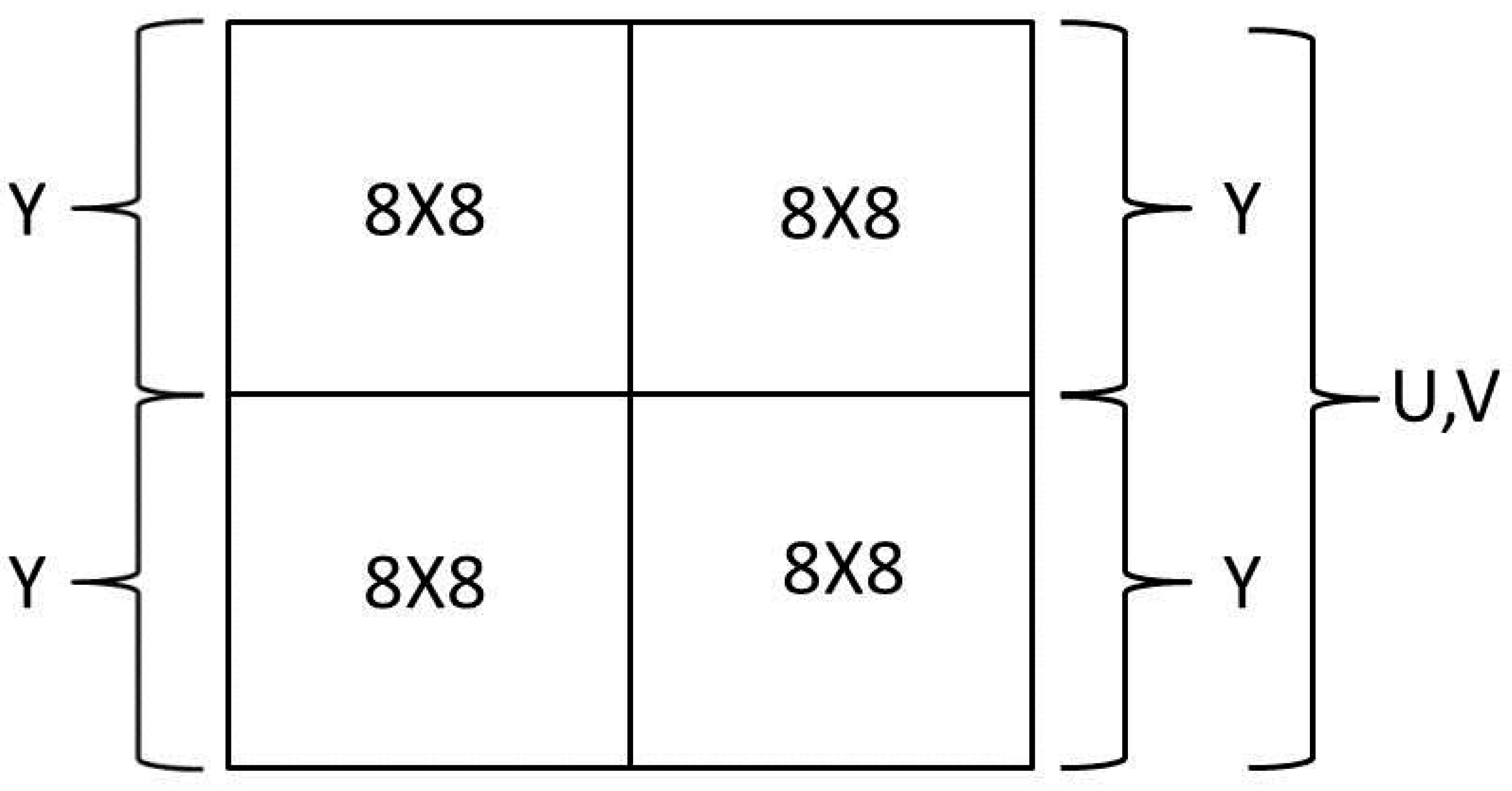
A common practice is a quartered resolution of the U data and the V data, which is called 4:1:1 chroma subsampling [12]. This 4:1:1 denotes there are four times more luminance data than the chrominance data. In other words, for each block of 16 × 16 that can be divided to four blocks of 8 × 8, as shown in Figure 1, there are four Y blocks and just one U block and one V block. Each row in an H.264 frame consists of lines of Y, U, and V blocks. The lines are positioned from top to bottom, where the blocks of each line are from left to right.
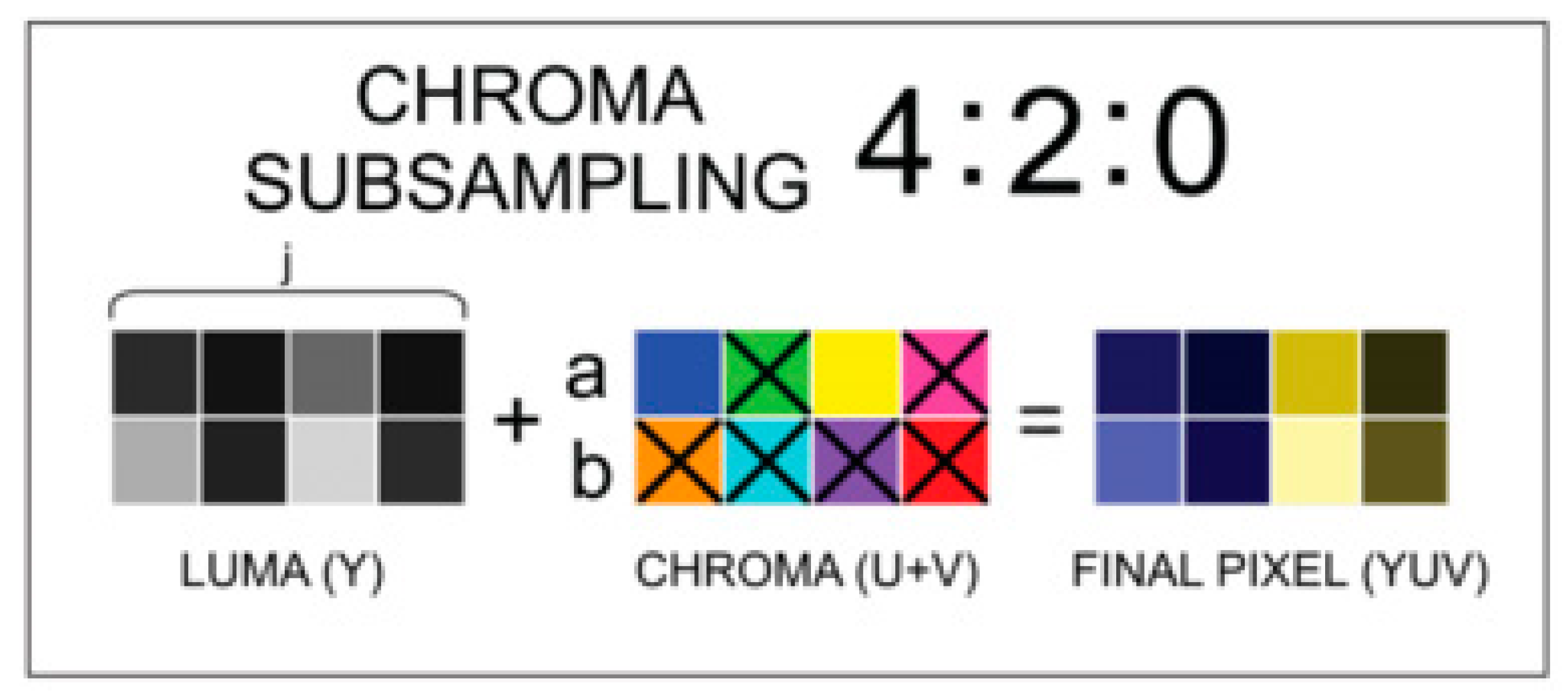
However, another chroma subsampling procedure of JPEG is very common. The 4:2:0 subsampling is very similar to 4:1:1. The 4:2:0 subsampling also keeps more information about the Y component and a smaller amount of information about the U and the V components. In 4:2:0 subsampling, the horizontal and the vertical sampling are different. The pixels of the U and the V components are sampled just on odd lines and not on even lines; however, in each sampled line, two pixels of each U and V component are sampled.
Figure 2 shows an example of the 4:2:0 subsampling. The six pixels marked with the letter X lose their original color and are replaced by the color of the upper-left pixel in the quad.
The compression ratios of 4:1:1 and 4:2:0 are roughly the same, and both of them are popular when using H.264 [14,15].
H.264 has three types of frames: I-frames, P-frames, and B-frames [16]:
- I-frames (intracoded frames)—standalone frames containing all the data required to show the frame. Actually, this frame is very similar to a JPEG still image [17].
- P-frames (predictive frames)—predicted from another decoded frame.
- B-frames (bidirectional predicted frames)—predicted from both a previously decoded frame and a yet-to-come decoded frame.
H.264 applies three steps to each block in each frame:
- Transform each block to a frequency space employing the forward discrete cosine transform (FDCT) [18].
- Employ quantization; i.e., each value is divided by a predefined quantization coefficient and next rounded to an integer value [19].
- Compress the file employing a version of canonical Huffman codes [20].
In order to decompress a frame, we have perform do the same operations as in compression, but in reverse order. That is, first decoding the Huffman codes, then multiplying by the constants by which we divided the coefficients in the quantization step, and finally performing the inverse discrete cosine transform (IDCT).
3. Motivation
Video is used for communication between vehicles for several reasons. First, there is information that cannot be conveyed in a still image, such as the direction of movement or speed, and must be added as additional information to the still image. In a video, on the other hand, the direction of movement and speed can be deduced from the video itself.
In addition, video is a more reliable format. Each frame in the video is also a kind of backup for its adjacent frames. If only one frame is damaged, the adjacent frames can compensate for the loss of one frame. Indeed, a large loss of frames will create a problem, but a small percentage of frame loss can be unnoticed.
When it comes to choosing the desired encoder, the H.264 format has several advantages. H.264 is a broadly supported codec [21]. H.264 is supported by numerous up-to-date video players and also by many modern-day devices. This feature means that V2V communication using H.264 can be employed by many brands of vehicles [22].
In addition, H.264 is a royalty-free codec [23]. That is, there is no need to pay licensing fees for using H.264. Therefore, also from an economic point of view, it is better to choose H.264, because, naturally, the public of vehicle users prefer to pay as little as possible.
Vehicular networks are still in their early stages, but their significant potential to upgrade transportation efficiency and safety is agreed upon. As this technology develops further, videos for vehicular networks are expected to become a standard element in these networks [24]. The suggested algorithm in this paper aimed at promoting the use of video in vehicular networks.
4. Reduced Image Quality
H.264 was designed for the human eye and the quality level that people are able to see [25]. The level of quality that a vehicle needs to provide information for safety and the efficiency of its use is much lower. Actually, H.264 dedicates 24 bits for each pixel in the image, which allows for a very large range of colors and a high-quality image. A vehicle is able to perform well even with a much lower level of image quality. Reducing the number of bits from 24 to 3 lowers the image quality significantly; however, for what a vehicle needs, it is a sufficient quality.
Therefore, an algorithm is proposed that, on the one hand, will reduce the number of colors to only 8 frequent colors and, on the other hand, will not choose colors that are almost the same, but colors with high variance and that will finely represent the information in the original image for IoV. This algorithm for selecting the 8 most frequent colors is
| Algorithm 1 Selecting the 8 most frequent colors |
| Sort the colors by their count values. Take the top 8 colors. Calculate the variance of each pair of colors using Equation (1): Begin Find from the pair (x1,x2) the color with the smaller occurrences and remove it from the top 8 colors Add from the sorted list the next top color. Calculate the variances of the new color with the old colors End |
In Algorithm 1, are the RGB (red, green, blue) values of the first color, and are the RGB values of the second color. δ is the Feigenbaum constant [26].
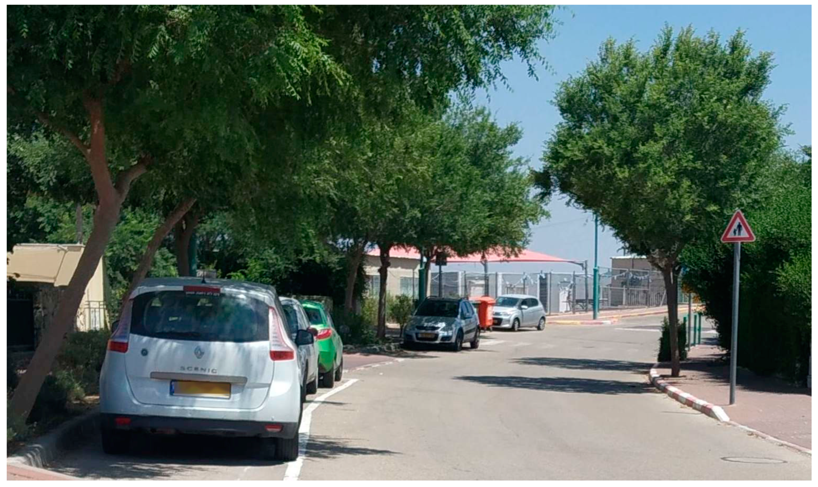
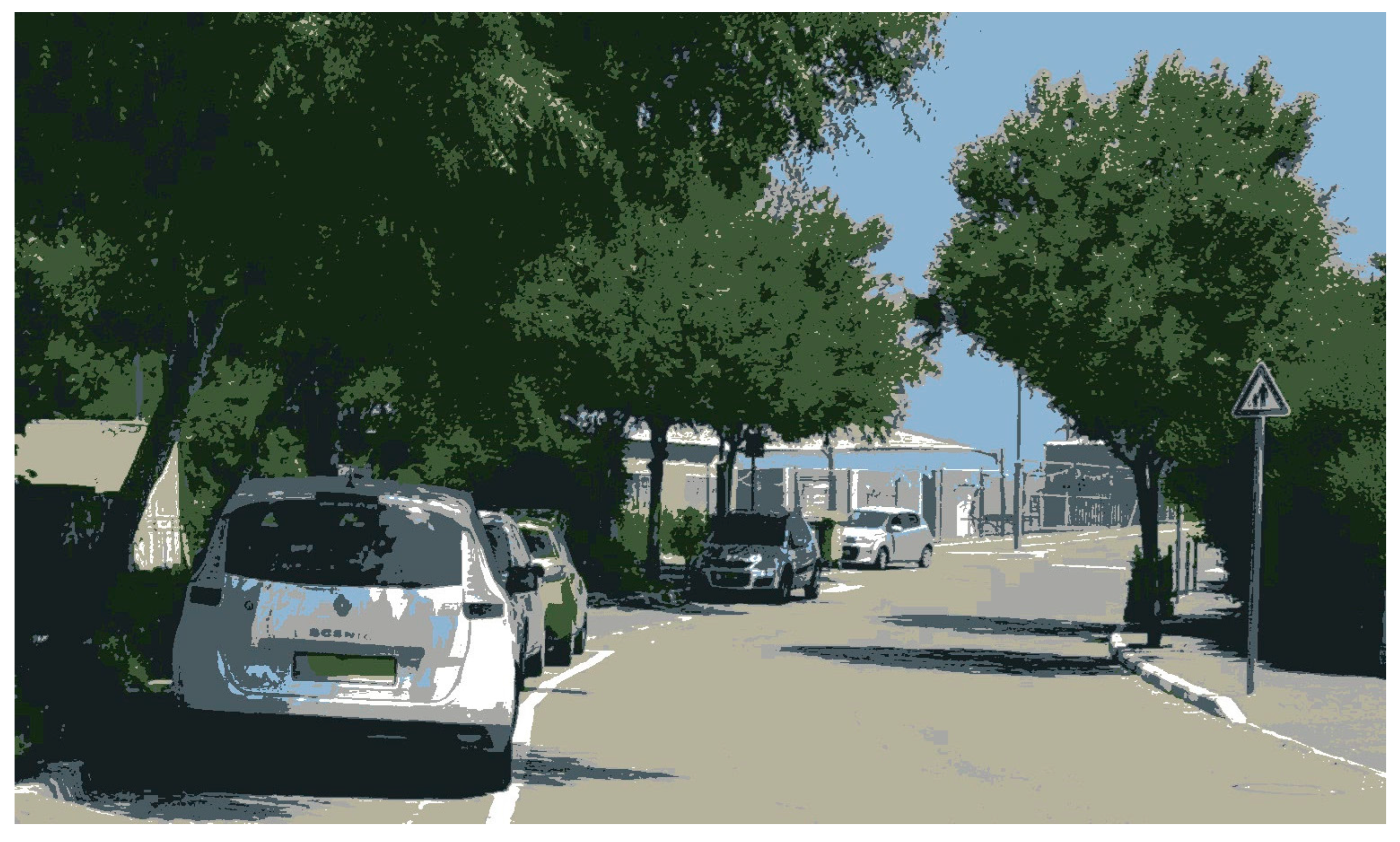
An example that shows the result of this algorithm is shown in Figure 3, Figure 4 and Figure 5. Figure 3 contains the original image. Figure 4 contains the edited picture according to Algorithm 1. Therefore, this figure contains only 8 colors. Figure 5 shows the selected colors and their probabilities in the edited picture.
For a vehicle, the essential data are observing other vehicles, the boundaries of the road, and recognizing the traffic signs. All of the essential tasks can be achieved with the 8-color image; nonetheless, the sending of the 8-color image on the vehicular network will be much faster because this image can be compressed better.
5. H.264 Quantization Tables
The reduced number of colors can be very helpful for a better compression ratio; however, H.264 assumes that the differences between the values within each frame are small, and the quantization tables of H.264 were formed according to this assumption. Hence, if we want to employ H.264, we must create different quantization tables that can fit frames with sharper changes.
In [27], the authors suggest quantization-optimized H.264 encoding for traffic video tracking applications. However, their suggestion does not support sharp changes, and it seems to be unsuitable for the approach in our paper.
The standard quantization tables of 90%, which are frequently used in vehicular networks, are shown in Table 1 and Table 2.
These default quantization tables were developed assuming that the possibility of sharp changes in the image will not often come out. This assumption is correct for regular images; however, the images of our application have a different kind of information containing more sharp changes. Therefore, although putting smaller numbers in the upper-left part of the quantization tables can be suitable for our application, the large values in the lower-right part of the quantization table can be harmful. The lower-right part of the quantization tables consists of data in relation to the sharper changes, and dividing this part’s values by such large numbers will cause a significant amount of data to be lost. Therefore, in blocks of images that contain sharp changes, the difference between the values of the upper-left part and the values of the lower-right part in the quantization tables must be reduced.
The standard quantization tables of 90% have significant disparity between the highest value in the table and the smallest value in the table. In the luminance quantization table, the values’ range is from 2 to 20, which represents a 10-fold difference. The chrominance quantization table has a smaller disparity, but still, the disparity is significant.
Other standard quantization tables of less than 90% can have even a larger disparity and can be even more than 10-fold. In our application, there are sharp changes in the images, and such disparity should be lowered.
Accordingly, attuning the quantization tables for our application that has sharp changes is essential because such an alteration of the quantization tables can enhance the compression ratio.
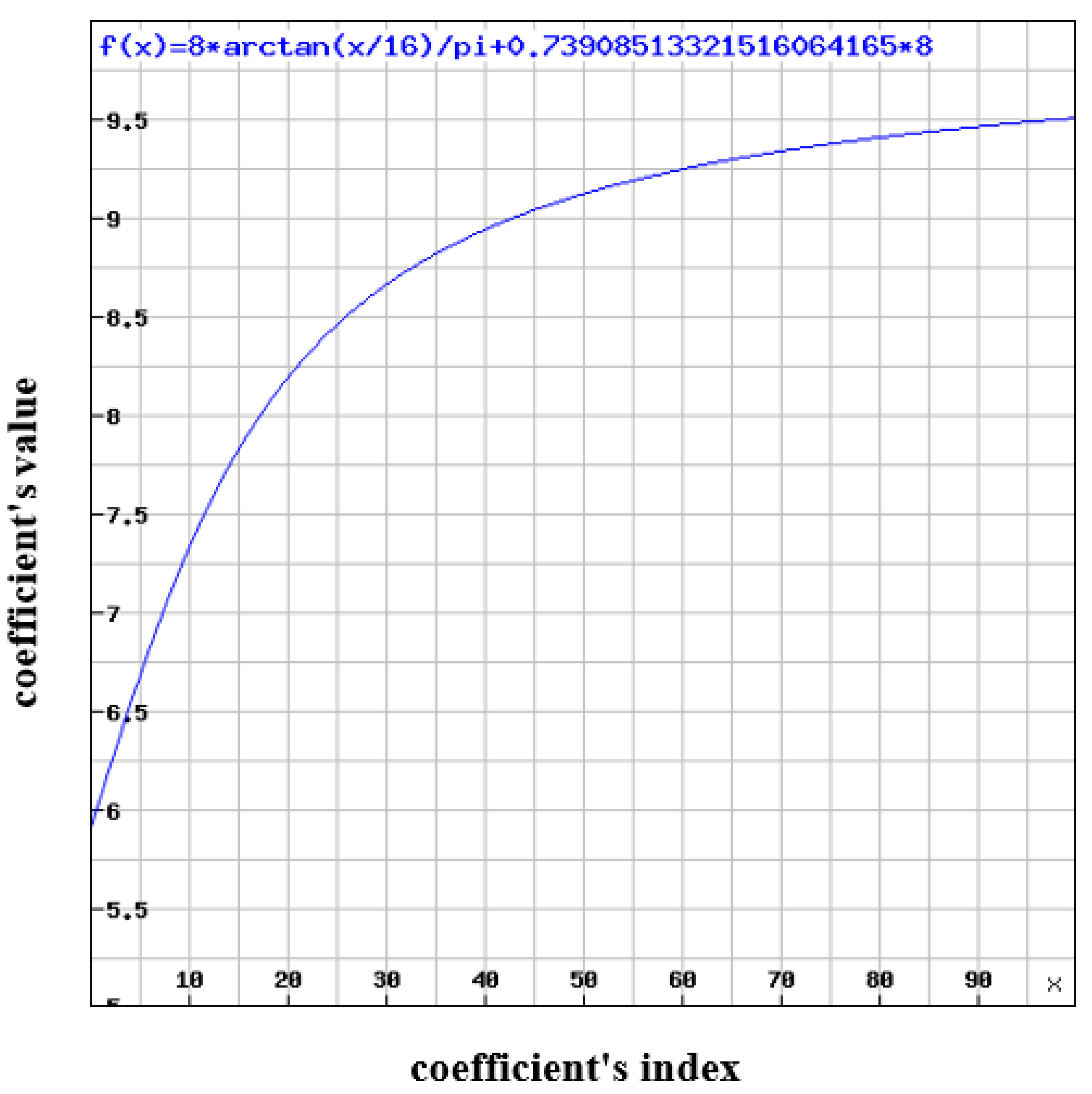
Typically, there is still disparity between the lower-right part and the upper-left part of H.264 blocks in our application; however, the disparity is slighter. Therefore, this formula is recommended for the luminance component:
where . X is the coefficient’s index in the X-axis, and Y is the coefficient’s index in the Y-axis; f(x) is the coefficient’s value in the quantization table.
DOTTIE is the Dottie number [28]. The Dottie number is the unique real fixed point of the cosine function. In other words, if the cosine function is repeatedly applied to a random number, it will generate a sequence that will converge to the Dottie number.
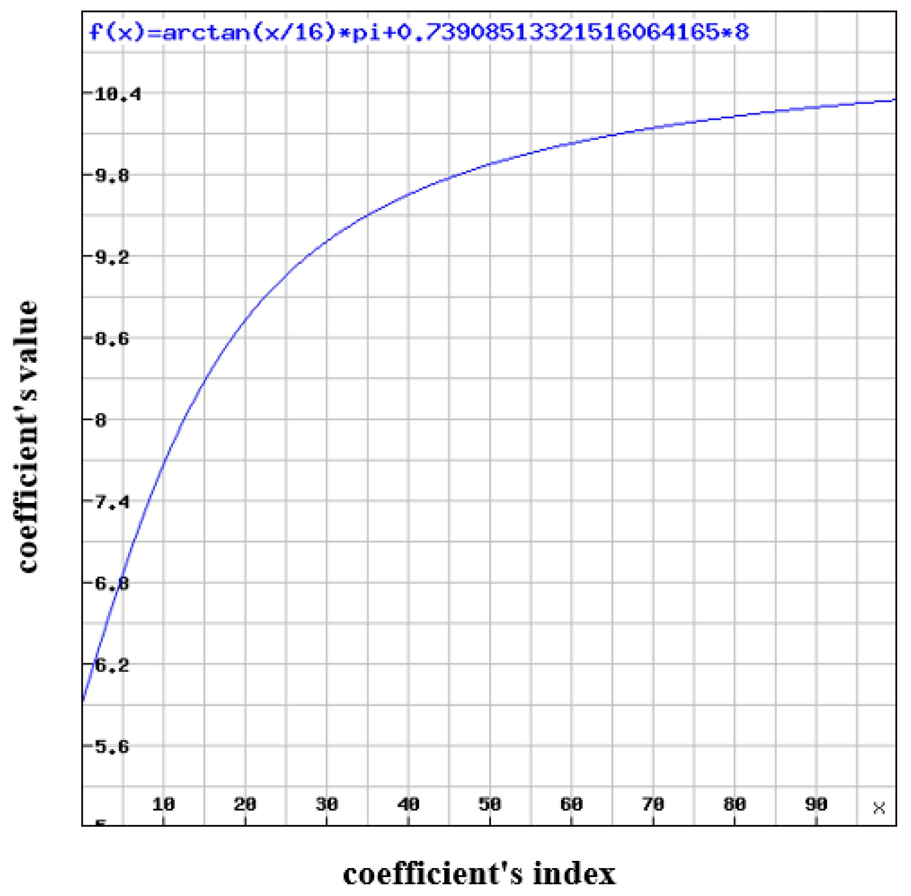
Similarly, this formula is recommended for the chrominance component:
where . X is the coefficient’s index in the X-axis, and Y is the coefficient’s index in the Y-axis; f(x) is the coefficient’s value in the quantization table.
DOTTIE is the Dottie number.
The graphs of the recommended formulas are shown in Figure 6 and Figure 7. These graphs were generated using [29].
The quantization tables that were calculated according to these formulas are shown in Table 3 and Table 4.
H.264 does not support real numbers for the quantization tables. The developers of H.264 decided about this because real numbers give a resolution that is good enough. There is no need for the real numbers’ better precision that would result in less good compression to obtain a quality that the human eye cannot distinguish. In our application, we are even willing to further decrease the quality of the image, so clearly, we do not need the exactness of the real numbers. Therefore, we rounded the real numbers to natural numbers, and thus, the table we created contains only natural numbers.
The curve of the graphs starts low and then increases because the functions are based on the tangent function, which starts low and then increases for the reason that the ratio of the opposite leg to the adjacent leg increases as the angle increases.
It can be easily seen that the disparity of the values in the suggested quantization tables is much smaller. From a disparity of 10-fold, we moved toward a disparity of less than 2-fold. This disparity might not be suitable for a regular frame of H.264; however, for this specific application, it is much more suitable.
6. Results
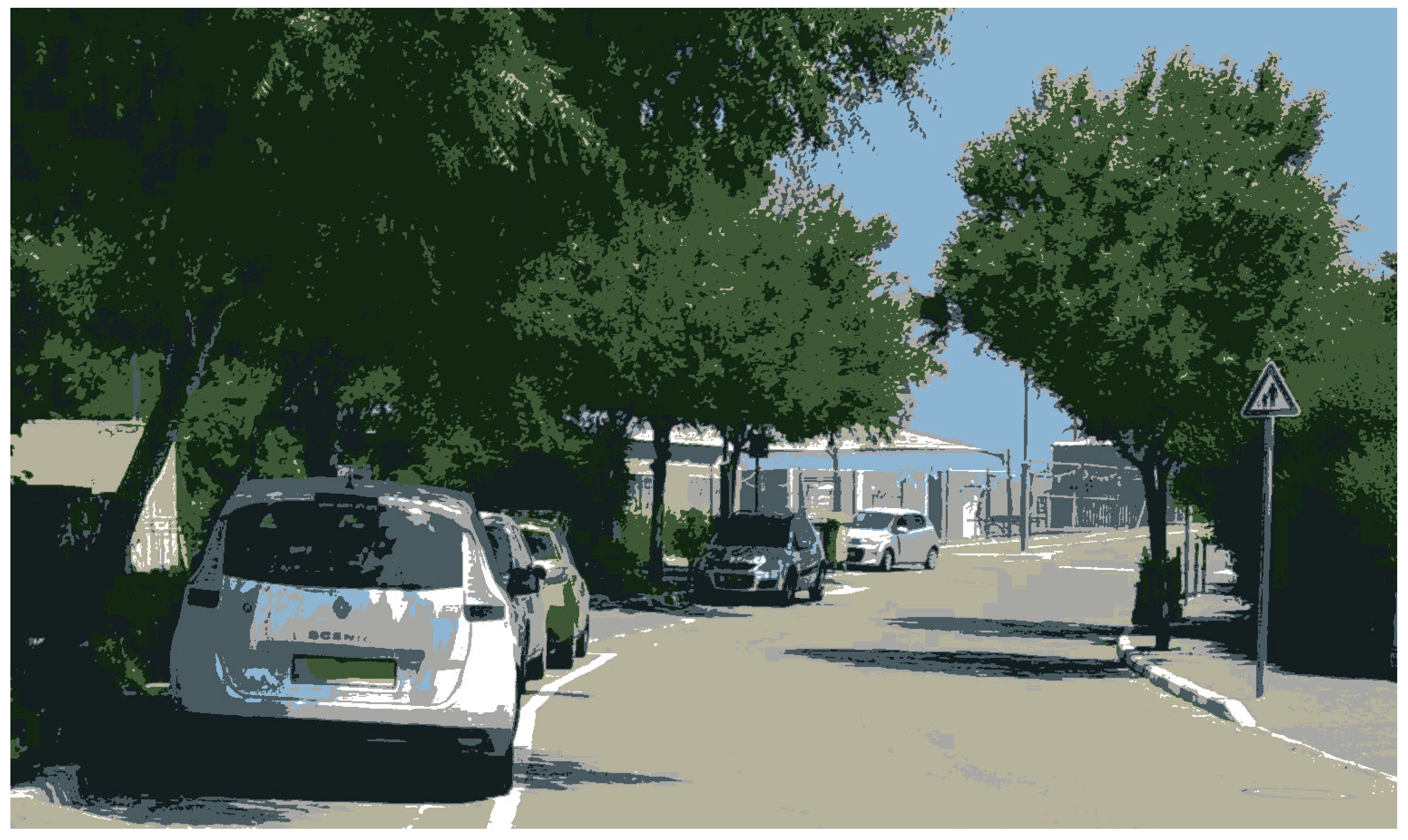
We used Figure 3 and Figure 4 for assessing the effectiveness of the suggested technique. When shifting from a full-color image to an 8-color image, many components of the information were removed. Therefore, the image size was reduced from 382,874 bytes to 260,600 bytes, which is a reduction of 31.936%.
When we changed the quantization table to the suggested quantization tables that are suitable to an image with sharp changes, the size of the image was reduced to 204,798 bytes, which is a total decrease of 46.510%.
The new constructed image is shown in Figure 8. It is fine enough for a vehicle, and as mentioned, it is almost half in its size; therefore, this image can be transmitted much faster.
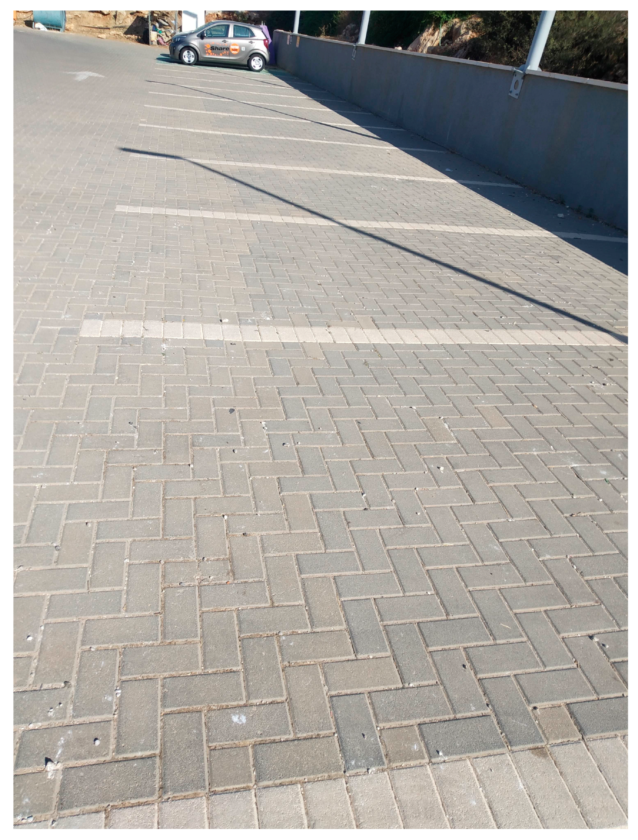
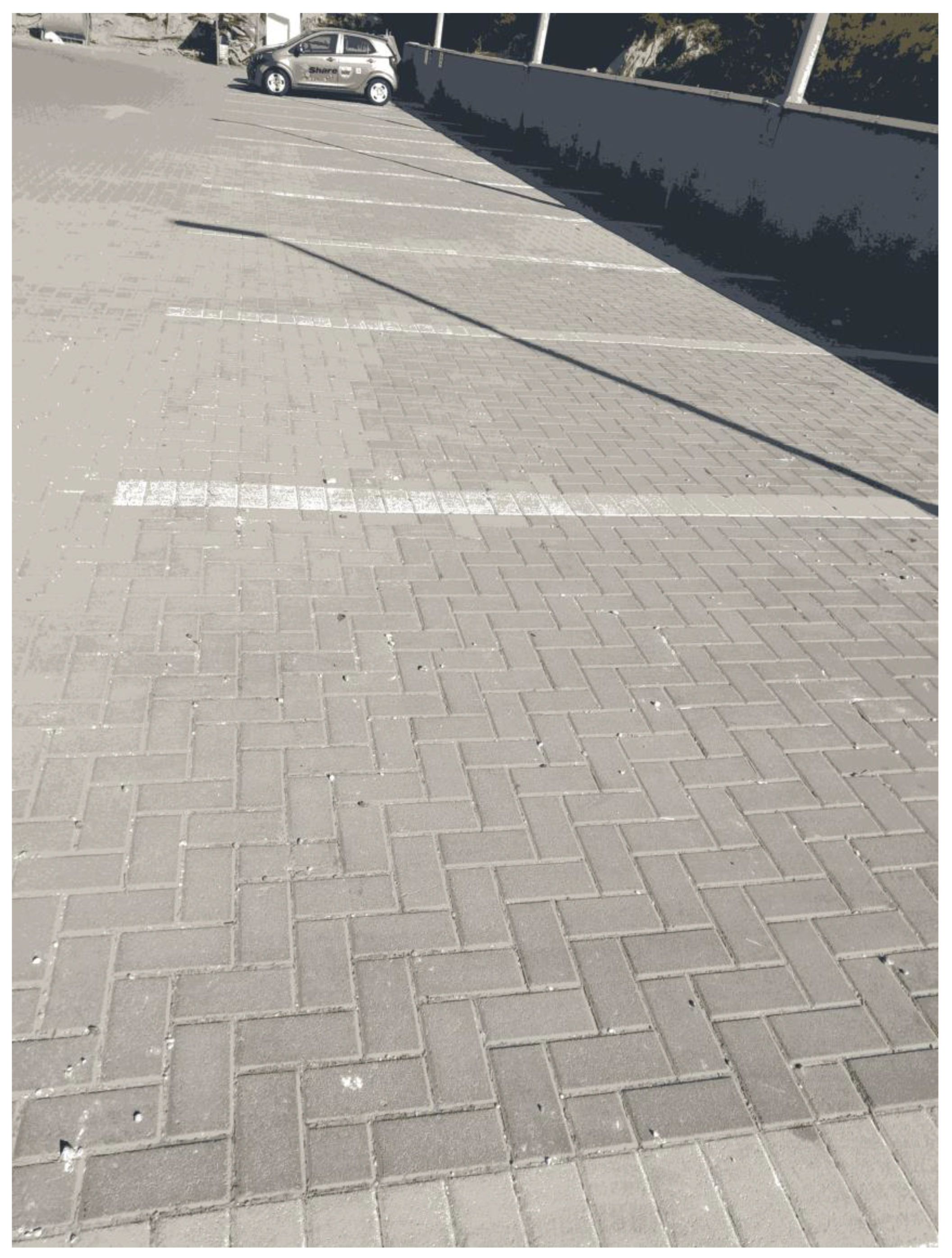
We tried the suggested technique also on a larger image of 3,055,616 bytes. The image is of a parking lot and is shown in Figure 9.
In this image, the moving to 8 colors made only minor changes to the image, mostly in the upper part of the image, which has some different colors. The size of the original picture was reduced by 35.154% to just 1,981,449 bytes when modifying to an 8-color image, because the original image had some minor changes that were removed in the 8-color image. The cases of no change are the best cases for the compression algorithm of H.264, which will generate the smaller files in such cases. Therefore, there is a large gain in Figure 10.
The shifting to the new suggested quantization tables also contributes an additional reduction in file size. The new file size is 1,755,971 bytes, which is a total decrease of 42.533%.
In this image, the contribution of the new suggested quantization tables was much smaller, because the file already had many zeros, which indicate “no change”. It does not matter if we divide the zero in the quantization step by a small or a large number. Dividing zero by any number will yield zero, so the efficiency of the original quantization tables and the new suggested quantization tables will be the same in the cases of a zero value.
The new image, which has only unnoticed change, is shown in Figure 11.
The results of the two images’ compression are summarized in Table 5.
7. Conclusions
Reducing data transmission in vehicle networks is imperative when many vehicles turn to smart driving [30]. We have proposed two steps to reduce the amount of data transmitted on vehicle networks.
Step 1: Reduce Color Resolution
The first step is to reduce the color resolution of images from full color to 8 colors. This may seem like a significant reduction, but it is still sufficient for most vehicle applications. For example, traffic lights and road signs can be easily distinguished in 8 colors.
Step 2: Modify Quantization Tables
The second step is to modify the quantization tables used by the H.264 video codec. Quantization tables are used to reduce the amount of data required to represent an image. By modifying the quantization tables, we can further reduce the amount of data required to transmit 8-color images.
The combination of these two steps can reduce the amount of data transmitted by almost 50%. This can significantly improve the efficiency of vehicle networks.
Funding
This research received no external funding.
Institutional Review Board Statement
Not applicable.
Informed Consent Statement
Not applicable.
Data Availability Statement
Not applicable.
Conflicts of Interest
The authors declare no conflict of interest.
References
- Punchihewa, A.; Bailey, D. A Review of Emerging Video Codecs: Challenges and Opportunities. In Proceedings of the 2020 35th IEEE International Conference on Image and Vision Computing New Zealand (IVCNZ), Wellington, New Zealand, 25–27 November 2020; pp. 1–6. [Google Scholar]
- Lu, Y.; Li, S. A review on developing status of stereo video technology. In Proceedings of the 2012 IEEE International Conference on Computer Science and Information Processing (CSIP), Xi’an, China, 24–26 August 2012; pp. 715–718. [Google Scholar]
- Bahri, N.; Werda, I.; Grandpierre, T.; Ayed MA, B.; Masmoudi, N.; Akil, M. Optimizations for real-time implementation of H.264/AVC video encoder on DSP processor. Int. Rev. Comput. Softw. (IRECOS) 2013, 8, 2025–2035. [Google Scholar]
- Kang, K.D. A Review of Efficient Real-Time Decision Making in the Internet of Things. Technologies 2022, 10, 12. [Google Scholar] [CrossRef]
- Wiseman, Y. Autonomous vehicles. In Research Anthology on Cross-Disciplinary Designs and Applications of Automation; IGI Global: Hershey, PA, USA, 2022; pp. 878–889. [Google Scholar]
- Liu, X.; Li, Y.; Dai, C.; Li, P.; Yang, L.T. An efficient H. 264/AVC to HEVC transcoder for real-time video communication in Internet of Vehicles. IEEE Internet Things J. 2018, 5, 3186–3197. [Google Scholar] [CrossRef]
- Budati, A.K.; Islam, S.; Hasan, M.K.; Safie, N.; Bahar, N.; Ghazal, T.M. Optimized Visual Internet of Things for Video Streaming Enhancement in 5G Sensor Network Devices. Sensors 2023, 23, 5072. [Google Scholar] [CrossRef] [PubMed]
- Zhou, J.; Zhou, D.; Zhang, H.; Hong, Y.; Liu, P.; Goto, S. A 136 cycles/MB, luma-chroma parallelized H. 264/AVC deblocking filter for QFHD applications. In Proceedings of the 2009 IEEE International Conference on Multimedia and Expo, New York, NY, USA, 28 June–July 2009; pp. 1134–1137. [Google Scholar]
- Sharrab, Y.O.; Sarhan, N.J. Detailed comparative analysis of vp8 and h. 264. In Proceedings of the 2012 IEEE International Symposium on Multimedia, Irvine, CA, USA, 10–12 December 2012; pp. 133–140. [Google Scholar]
- Ho, Y.H.; Lin, C.H.; Chen, P.Y.; Chen, M.J.; Chang, C.P.; Peng, W.H.; Hang, H.M. Learned video compression for yuv 4:2:0 content using flow-based conditional inter-frame coding. In Proceedings of the 2022 IEEE International Symposium on Circuits and Systems (ISCAS), Austin TX, USA, 28 May–1 June 2022; pp. 829–833. [Google Scholar]
- Gunjal, B.L.; Mali, S.N. Comparative performance analysis of DWT-SVD based color image watermarking technique in YUV, RGB and YIQ color spaces. Int. J. Comput. Theory Eng. 2011, 3, 714. [Google Scholar] [CrossRef] [Green Version]
- Sinha, A.K.; Mishra, D. Deep Video Compression using Compressed P-Frame Resampling. In Proceedings of the 2021 National Conference on Communications (NCC), Virtual Conference, 7–30 July 2021; pp. 1–6. [Google Scholar]
- KVMGalore. 2023. Available online: http://kb.kvmgalore.com/lookup/ (accessed on 9 May 2023).
- Hsia, S.C.; Chou, Y.C. VLSI implementation of high-throughput parallel H. 264/AVC baseline intra-predictor. IET Circuits Devices Syst. 2014, 8, 10–18. [Google Scholar] [CrossRef]
- Dumic, E.; Mustra, M.; Grgic, S.; Gvozden, G. Image quality of 4:2:2 and 4:2:0 chroma subsampling formats. In Proceedings of the 2009 IEEE international symposium ELMAR, Zadar, Croatia, 28–30 September 2009; pp. 19–24. [Google Scholar]
- Shahid, Z.; Chaumont, M.; Puech, W. Fast protection of H. 264/AVC by selective encryption of CAVLC and CABAC for I and P frames. IEEE Trans. Circuits Syst. Video Technol. 2011, 21, 565–576. [Google Scholar]
- Park, J.H.; Lee, S.H.; Lim, K.S.; Kim, J.H.; Kim, S. A flexible transform processor architecture for multi-CODECs (JPEG, MPEG-2, 4 and H. 264). In Proceedings of the 2006 IEEE International Symposium on Circuits and Systems (ISCAS), Kos, Greece, 21–24 May 2006. [Google Scholar]
- Okade, M.; Mukherjee, J. Discrete Cosine Transform: A Revolutionary Transform That Transformed Human Lives [CAS 101]. IEEE Circuits Syst. Mag. 2022, 22, 58–61. [Google Scholar]
- Malvar, H.S.; Hallapuro, A.; Karczewicz, M.; Kerofsky, L. Low-complexity transform and quantization in H. 264/AVC. IEEE Trans. Circuits Syst. Video Technol. 2003, 13, 598–603. [Google Scholar]
- Klein, S.T.; Wiseman, Y. Parallel Huffman decoding with applications to JPEG files. Comput. J. 2003, 46, 487–497. [Google Scholar] [CrossRef] [Green Version]
- Vetro, A.; Wiegand, T.; Sullivan, G.J. Overview of the stereo and multiview video coding extensions of the H. 264/MPEG-4 AVC standard. Proc. IEEE 2011, 99, 626–642. [Google Scholar] [CrossRef] [Green Version]
- Abou-Zeid, H.; Pervez, F.; Adinoyi, A.; Aljlayl, M.; Yanikomeroglu, H. Cellular V2X transmission for connected and autonomous vehicles standardization, applications, and enabling technologies. IEEE Consum. Electron. Mag. 2019, 8, 91–98. [Google Scholar]
- Ravi, A.; Rao, K.R. Performance analysis comparison of the Dirac video codec with H 264/MPEG-4 Part 10 AVC. Int. J. Wavelets Multiresolut. Inf. Process. 2011, 9, 635–654. [Google Scholar] [CrossRef] [Green Version]
- Jiang, X.; Yu, F.R.; Song, T.; Leung, V.C. Resource allocation of video streaming over vehicular networks: A survey, some research issues and challenges. IEEE Trans. Intell. Transp. Syst. 2021, 23, 5955–5975. [Google Scholar] [CrossRef]
- Amor, M.B.; Kammoun, F.; Masmodi, N. A pretreatment using saliency map Harris to improve MSU blocking metric performance for encoding H. 264/AVC: Saliency map for video quality assessment. In Proceedings of the 2016 IEEE International Image Processing, Applications and Systems (IPAS), Hammamet, Tunisia, 5–7 November 2016; pp. 1–4. [Google Scholar]
- Briggs, K. A precise calculation of the Feigenbaum constants. Math. Comput. 1991, 57, 435–439. [Google Scholar]
- Soyak, E.; Tsaftaris, S.A.; Katsaggelos, A.K. Quantization optimized H. 264 encoding for traffic video tracking applications. In Proceedings of the 2010 IEEE International Conference on Image Processing, Hong Kong, 26–29 September 2010; pp. 1241–1244. [Google Scholar]
- Wiseman, Y. JPEG Quantization Tables for GPS Maps. Autom. Control. Comput. Sci. 2021, 55, 568–576. [Google Scholar] [CrossRef]
- Rechneronline. Draw Function Graphs. 2023. Available online: https://rechneronline.de/function-graphs/ (accessed on 9 May 2023).
- Yaqoob, I.; Khan, L.U.; Kazmi, S.A.; Imran, M.; Guizani, N.; Hong, C.S. Autonomous driving cars in smart cities: Recent advances, requirements, and challenges. IEEE Netw. 2019, 34, 174–181. [Google Scholar] [CrossRef]
Figure 1.
H.264 block of 16 × 16.

Figure 2.
4:2:0 subsampling layout [13].
Figure 2.
4:2:0 subsampling layout [13].

Figure 3.
An original full-color image of a street.

Figure 4.
The same image of a street but with only 8 colors.

Figure 5.
The distribution of the selected 8 colors.

Figure 6.
Luminance quantization table’s graph.

Figure 7.
Chrominance quantization table’s graph.

Figure 8.
The image of a street with 8 colors and the suggested quantization tables.

Figure 9.
Image of a parking lot with full color.

Figure 10.
Image of a parking lot with 8 colors.

Figure 11.
Image of a parking lot with 8 colors and the suggested quantization tables.


Table 1.
H.264 luminance quantization table of 90%.
| 3 | 2 | 2 | 3 | 5 | 8 | 10 | 12 |
| 2 | 2 | 3 | 4 | 5 | 12 | 12 | 11 |
| 3 | 3 | 3 | 5 | 8 | 11 | 14 | 11 |
| 3 | 3 | 4 | 6 | 10 | 17 | 16 | 12 |
| 4 | 4 | 7 | 11 | 14 | 22 | 21 | 15 |
| 5 | 7 | 11 | 13 | 16 | 21 | 23 | 18 |
| 10 | 13 | 16 | 17 | 21 | 24 | 24 | 20 |
| 14 | 18 | 19 | 20 | 22 | 20 | 21 | 20 |
Table 2.
H.264 chrominance quantization table of 90%.
| 3 | 4 | 5 | 9 | 20 | 20 | 20 | 20 |
| 4 | 4 | 5 | 13 | 20 | 20 | 20 | 20 |
| 5 | 5 | 11 | 20 | 20 | 20 | 20 | 20 |
| 9 | 13 | 20 | 20 | 20 | 20 | 20 | 20 |
| 20 | 20 | 20 | 20 | 20 | 20 | 20 | 20 |
| 20 | 20 | 20 | 20 | 20 | 20 | 20 | 20 |
| 20 | 20 | 20 | 20 | 20 | 20 | 20 | 20 |
| 20 | 20 | 20 | 20 | 20 | 20 | 20 | 20 |
Table 3.
Luminance quantization table according to the suggested formula.
| 6 | 6 | 6 | 6 | 8 | 8 | 9 | 9 |
| 6 | 6 | 6 | 6 | 8 | 8 | 9 | 9 |
| 6 | 6 | 6 | 6 | 8 | 8 | 9 | 9 |
| 6 | 6 | 6 | 8 | 8 | 9 | 9 | 9 |
| 8 | 8 | 8 | 8 | 9 | 9 | 9 | 9 |
| 8 | 8 | 8 | 9 | 9 | 9 | 9 | 9 |
| 9 | 9 | 9 | 9 | 9 | 9 | 9 | 9 |
| 9 | 9 | 9 | 9 | 9 | 9 | 9 | 9 |
Table 4.
Chrominance quantization table according to the suggested formula.
| 6 | 6 | 6 | 6 | 8 | 8 | 9 | 10 |
| 6 | 6 | 6 | 6 | 8 | 8 | 9 | 10 |
| 6 | 6 | 6 | 6 | 8 | 8 | 9 | 10 |
| 6 | 6 | 6 | 8 | 8 | 9 | 9 | 10 |
| 8 | 8 | 8 | 8 | 9 | 9 | 10 | 10 |
| 8 | 8 | 8 | 9 | 9 | 10 | 10 | 10 |
| 9 | 9 | 9 | 9 | 10 | 10 | 10 | 10 |
| 10 | 10 | 10 | 10 | 10 | 10 | 10 | 10 |
Table 5.
Compression’s results of the images.
| Image | Reduction after the First Step | Reduction after the Second Step |
|---|---|---|
| Road | 31.936% | 46.510% |
| Parking lot | 35.154% | 42.533% |
Disclaimer/Publisher’s Note: The statements, opinions and data contained in all publications are solely those of the individual author(s) and contributor(s) and not of MDPI and/or the editor(s). MDPI and/or the editor(s) disclaim responsibility for any injury to people or property resulting from any ideas, methods, instructions or products referred to in the content. |
© 2023 by the author. Licensee MDPI, Basel, Switzerland. This article is an open access article distributed under the terms and conditions of the Creative Commons Attribution (CC BY) license (https://creativecommons.org/licenses/by/4.0/).
Share and Cite
MDPI and ACS Style
Wiseman, Y. Adapting the H.264 Standard to the Internet of Vehicles. Technologies 2023, 11, 103. https://doi.org/10.3390/technologies11040103
AMA Style
Wiseman Y. Adapting the H.264 Standard to the Internet of Vehicles. Technologies. 2023; 11(4):103. https://doi.org/10.3390/technologies11040103
Chicago/Turabian StyleWiseman, Yair. 2023. "Adapting the H.264 Standard to the Internet of Vehicles" Technologies 11, no. 4: 103. https://doi.org/10.3390/technologies11040103
Note that from the first issue of 2016, this journal uses article numbers instead of page numbers. See further details here.