Article

Mobilenetv2_CA Lightweight Object Detection Network in Autonomous Driving

1
School of Mechanical Engineering, Anhui Polytechnic University, Wuhu 241000, China
2
Polytechnic Institute, Zhejiang University, Hangzhou 310027, China
*
Author to whom correspondence should be addressed.
Technologies 2023, 11(2), 47; https://doi.org/10.3390/technologies11020047
Submission received: 5 February 2023 / Revised: 1 March 2023 / Accepted: 21 March 2023 / Published: 23 March 2023
(This article belongs to the Special Issue Image and Signal Processing)

Abstract

:
A lightweight network target detection algorithm was proposed, based on MobileNetv2_CA, focusing on the problem of high complexity, a large number of parameters, and the missed detection of small targets in the target detection network based on candidate regions and regression methods in autonomous driving scenarios. First, Mosaic image enhancement technology is used in the data pre-processing stage to enhance the feature extraction of small target scenes and complex scenes; second, the Coordinate Attention (CA) mechanism is embedded into the Mobilenetv2 backbone feature extraction network, combined with the PANet and Yolo detection heads for multi-scale feature fusion; finally, a Lightweight Object Detection Network is built. The experimental test results show that the designed network obtained the highest average detection accuracy of 81.43% on the Voc2007 + 2012 dataset, and obtained the highest average detection accuracy of 85.07% and a detection speed of 31.84 FPS on the KITTI dataset. The total amount of network parameters is only 39.5 M. This is beneficial to the engineering application of MobileNetv2 network in automatic driving.

1. Introduction

With the development of autonomous driving technology in recent years, object detection has become a research focus in the field of autonomous driving, and it is crucial to achieve the fast and accurate detection of common objects in real traffic scenes. Traditional object detection algorithms usually rely on specific application scenarios and manually designed features with poor generalization abilities [1,2]. With the wide application of Convolutional Neural Networks (CNN) in the field of computer vision in recent years, object detection based on CNN [3,4,5] has achieved an excellent performance. Ge Z et al. [6] balanced the detection accuracy and speed using the decoupled head decoupling head, anchor free method and SimOTA sample selection method. Xu S et al. [7] used the efficient task alignment head, advanced label assignment strategy and fine-grained objective loss function, which implements an efficient object detector. However, traditional CNN usually requires a large quantity of parameters to achieve satisfactory precision. Liu Z et al. [8] created a convolution-free model for image classification by stacking multiple Transformer blocks to process sequences of non-overlapping image patches. Compared with the CNN-based model, the Transformer-based model has a larger receptive field but requires a system with a large amount of training data and model parameters to achieve superior performance. The redundant attention (Attention) in the Transformer will also lead to a huge computational cost. This is extremely unhelpful to deploying the model on an autonomous driving platform. In real embedded autonomous driving platforms, the design trend in the neural network is to explore lightweight and efficient network architectures with an acceptable performance for mobile devices to improve network detection efficiency.
For the lightweight design of neural networks, it is common practice to compress the existing convolutional neural networks or design a new lightweight network architecture. Han S et al. [9] proposed the use of network pruning to prune unimportant weights in neural networks, which reduces a large quantity of parameters in the fully connected layer by weight pruning, but may not sufficiently reduce the computational cost of the convolutional layer due to the irregular sparsity in the pruned network. Li H et al. [10] pruned filters to obtain effective CNNs using l 1 parametric regularization; these filters are considered to have little impact on the output precision, which reduces the calculation cost by removing the overall filters in the network and its connected feature maps. This approach does not lead to sparse connectivity patterns compared to the pruning weights shown in the literature [9]. Rastegari M et al. [11] quantified the weights and activations as 1-bit data, while the filter and convolution layers, improved to binary, use binary operations to approximate convolution, achieving a certain degree of compression and acceleration ratio. However, the overall parametric reduction in the network is not significant. Hinton G et al. [12] introduced the knowledge distillation method. This transfers the knowledge from the larger model to the smaller model, which leads to a poor generalization ability within the whole network. Han K et al. [13] used a new Ghost module, which first controls the total number of ordinary convolutions and then generates more feature maps using linear operations to reduce the total number of parameters without changing the size of the feature maps. These methods of compressing the existing convolutional neural networks usually mean that the convolutional neural networks tend to be shallow. The detection efficiency of shallow neural networks is generally far lower than that of deep neural networks, and will be limited by the pre-trained deep neural networks used as the baseline. Therefore, to reduce the complexity of the network while achieving both good detection precision and speed, a future development trend is to redesign a lightweight network architecture with high efficiency.
The main idea of designing a lightweight neural network architecture is to design a more efficient network structure by optimizing the computational method of convolution to effectively reduce the computational effort during convolutional computation. Iandola F N et al. [14] proposed the SqueezeNet network, which is constructed by the basic module of Fire module, in which the Squeeze layer uses 1 × 1 convolutional kernels to reduce the number of parameters, and the Expand layer uses 1 × 1 and 3 × 3 convolutional kernels to obtain the corresponding feature maps and then stitch them together to obtain the output of the Fire module. However, this has a weak efficiency for complex problems due to the low number of parameters. Zhang X et al. [15] improved the conventional residual structure by replacing the first 1 × 1 convolution layer that is connected to the input feature map with grouped convolution and using the Channel shuffle operation to interact information on the output results of each group of grouped convolutions, achieving a network performance with reduced computation. However, this produces a boundary effect; that is, an output channel comes from a small part of the input channel. Howard A.G [16] proposed replacing the general convolution layer with the depth separable convolution, which greatly reduces the network parameters; however, feature degradation occurs during the training process. Sandler M et al. [17] proposed resolving problem of feature degradation in MobileNetv1 using the inverted residual structure “dimension raising-convolution-dimension reduction”, and the depth separable convolution is used to reduce the calculation amount in the intermediate convolution operation and improve the efficiency of the convolution calculation. However, this convolution may not extract enough information about a small number of deep-level features.
Figure 1 clearly demonstrates the superiority of our model in terms of the number of network parameters and the average detection degree. Our algorithm achieved the highest detection accuracy with the lowest amount of network parameters, and has a good application prospect.
In this paper, based on previous research, we further explore the design of lightweight and high-precision object detection networks. Our contributions are as follows: (1) embed coordinate attention (CA) into the lightweight backbone feature extraction network MobileNetv2, which improves the backbone feature extraction network’s ability to initially extract features; (2) accurately integrate the improved combination of the backbone feature extraction network and the multi-scale feature fusion network (PANet), which further enriches the network’s ability to extract location information and semantic information; (3) fast and accurate target detection is realized on the autonomous driving dataset KITTI, which is beneficial to the algorithm during automatic driving applications.

2. Algorithm Design

To achieve a lightweight object detection network with high precision and speed for object detection, a lightweight network model based on MobileNetv2_CA was proposed. The overall structure of the network model is shown in Figure 2. First, the improved lightweight Mobilenetv2 [17] network was used as the backbone feature extraction network for preliminary feature extraction, and the coordinated attention mechanism (CA) [18] was embedded to adaptively extract the channel relationships and location information to enrich feature extraction. Then, features at different scales were used as inputs for maximum pooling at different scales in the SPP [19] module to isolate significant contextual features, and the features were fed into the PANet [20] network for further enhanced feature extraction and multi-scale fusion. Finally, the three enhanced feature layers that were processed by, and input into, several convolutions were processed by 3 × 3 convolutional feature integration and 1 × 1 convolutional adjustment of the number of channels using the Yolo [5] detection head to obtain the prediction results. After decoding, score ranking and a non-maximum suppression screening of the prediction results, the detection results were obtained. The entire network combines the advantages of lightweight convolutional neural networks, a coordinate attention (CA) mechanism and the PANet multi-scale feature fusion network to construct an efficient and lightweight object detection network.

2.1. Pretreatment Stage

To reduce the network’s demand for device memory during feature extraction, and to enhance the feature extraction of small object scenes and multiple complex scenes, a novel Mosaic image enhancement method inspired by Yolov4 [21] was used in the data pre-processing stage. We experimentally determined the optimal scaling factor, original image warping ratio and channel warping for KITTI images. Scale represents the scaling ratio of the original image, which was set between 0.25 and 2 in this article. The jitter represents the distortion ratio of the width and height of the original image. In this article, we set jitter = 0.3, which means the distortion was between 0.7/1.3 (0.538) and 1.3/0.7 (1.857). Hue = 0.1, sat = 0.5 and val = 0.5, which represent the distortion of the three channels in the hsv color gamut, namely, hue (H), saturation (S) and lightness (V), respectively. These hyperparameters are related to image size, object class and density. The distribution of small object scenes and complex scenes in datasets was generally uneven, which meant that the learning of small objects and complex scenes in the training process was always less than adequate. By using the Mosaic image enhancement method, the possibility of obtaining multiple complex scenes and small object scenes after traversing four images greatly increases, which helps the network to accurately detect small objects and multiple complex scene targets by learning object features during the training process. The test results are shown in Figure 2.
Figure 3a shows the effect of data enhancement for small object scenes, and the small object in the distance was successfully captured. Figure 3b shows the effect of data enhancement for obscured objects and objects in low-light-state scenes, and the object in an obscured and low-light state was successfully captured. Figure 3c is the detection effect diagram of our model with Mosaic data enhancement turned off, and Figure 3d is the detection effect diagram of our model with Mosaic data enhancement turned on, which confirms that, if there is no data enhancement of the images, the detector will suffer from missed detections.

2.2. Improvement in Mobilenetv2 Backbone Network

To achieve the goal of a lightweight network, the backbone feature extraction network uses and improves MobileNetv2 [17]. The MobileNetV2 network model has a total of 17 Bottleneck layers (each Bottleneck contains two point-by-point convolutional layers and one depth convolutional layer), one standard convolutional layer (conv) and two point-by-point convolutional layers (pw conv), with a total of 54 trainable parameter layers. This is a series of Bottleneck layers stacked with different operation step stride(s). For repeated Bottleneck layers, generally only the first layer of s is 2, and the rest of the layers are 1.
When the Stride is 2, MobileNetv2 Bottleneck optimizes the network with a Linear Bottleneck Block. The fewer the number of channels in the feature map, the less the computation of the convolutional layer. However, it is difficult to extract enough feature information using only feature maps with a low number of channels. MobileNetV2 establishes a trade-off between these two, taking the 1 × 1 pointwise convolution to raise the dimension and using the Relu6 activation function instead of the Relu activation function. This is followed by 3 × 3 depth convolution and the use of the Relu6 activation function; then, 1 × 1 pointwise convolution is used to down-dimension and, after down-dimensioning, the linear activation function is used, the structure of which is shown in Figure 4. This convolution operation is beneficial to reduce the number of parameters.
When the Stride is 1, MobileNetv2 Bottleneck optimizes the network using the Inverted Residuals Block to enhance the feature extraction ability of MobileNetv2, a lightweight backbone feature extraction network, and causes the network to adaptively adjust the inter-channel relationship and location information to improve feature extraction. In this paper, the coordinate attention (CA) [18] mechanism proved to be an efficient attention mechanism. To demonstrate its advantages, different attention mechanisms are embedded in the same backbone network and trained and tested on the same dataset. The Pascal VOC [22] test set was used, and the object detection results are shown in Figure 5. When the same lightweight object detector—Yolov4Tiny—was used, the network adding our coordinated attention mechanism CA achieved the highest mAP of 77.54%, which is higher than the results achieved by SE [23], at 77.32% mAP, and CBAM [24], at 77.27% mAP. However, the parameter amount in the CA network was only 5.983 M, which is lower than the 6.004 M achieved by CBAM. Compared with SE, CA only increases the parameter amount by 0.02 M, but increases mAP by 0.22%. Compared with the other two attention mechanisms, SE and CBAM, the CA attention mechanism achieves the best detection at the cost of a small increase in the amount of parameters and is highly competitive. Inspired by this, we inserted this mechanism into the backbone network Mobilenetv2.
We embedded the mechanism in an Inverted Residuals Block, which is located between 3 × 3 deep convolution and 1 × 1 reduced-dimensional point convolution, forming the Inverted Residuals_CA Block. This was embedded into the Inverted Residuals Block using the following steps:
(1) In the channel attention, input X is given. Each channel was encoded along the horizontal and vertical coordinates using two spatial range pool kernels, (H,1) and (1, W), respectively. The output of the C-th channel at height H can be determined using Formula (1):
z c h ( h ) = 1 W 0 i < W x c ( h , i )
Similarly, the output of the C-th channel with width W can be determined using Formula (2):
z c w ( w ) = 1 H 0 j < H x c ( j , w )
The above two transformations aggregate features along two spatial directions, which helps the network to more accurately locate the objects of.
(2) After enabling the global receive field and encoding the exact location information using the aggregated feature mappings generated by Formulas (1) and (2), these were concatenated and input to the 1 × 1 convolutional transformation function f to generate Formula (3):
f = δ ( F 1 ( [ z h , z w ] ) )
wherein [] denotes the cascade operation along the spatial dimension, δ is the nonlinear activation function, f R C / r   × ( H + W ) is the intermediate feature mapping that horizontally and vertically encodes spatial information and r is the reduction rate of the control block size. f was divided into two independent tensors, f h R C / r   ×   H and f w R C / r   ×   W , along the spatial dimension. The other two 1 × 1 convolution transformations, F h and F w , were used to transform f h and f w into tensors with the same number of channels, which can be used to obtain Formulas (4) and (5), respectively:
g h = σ ( F h ( f h ) )
g w = σ ( F w ( f w ) )
wherein σ is sigmoid function. Outputs g h and g w were expanded. The output of the coordinate attention block Y can be formulated as Equation (6):
y c ( i , j ) = x c ( i , j ) × g c h ( i ) × g c w ( j )
Each element in the two attention mappings reflects the presence or absence of the object of interest in the corresponding row and column.
The structure of the Inverted Residuals_CA Block after embedding the Coordinate Attention (CA) mechanism is shown in Figure 6. This can first aggregate features along two spatial directions, and then encode the generated feature maps as a pair of direction-aware and position-sensitive attention maps. These attention maps can be complementarily applied to the input feature map to enhance the representation of the objects of interest and fully extract the feature information of the image.
After embedding the CA mechanism, the improved MobileNetv2 was renamed the MobileNetv2_CA network. A structural table is shown in Table 1. Input indicates the size of each module input in the network; operator denotes the modules experienced by each feature layer; t indicates the expansion factor, which is always applied to the input size; c indicates the number of channels output after passing through each feature layer; n indicates the number of bottlenecks; and s indicates the first-layer stride of each operation.
The network adaptive adjustment channel relationship and location information was extracted by MobileNetv2_CA backbone features, and the effective feature layer with the c = 32 output channels was extracted using the Inverted Residuals_CA Block at the seventh layer of the network when s = 1. The effective feature layer with c = 96 output channels was extracted using the Inverted Residuals_CA Block at the fourteenth layer of the network when s = 1. The effective feature layer with c = 320 output channels was extracted using the Inverted Residuals_CA Block at the eighteenth layer of the network when s = 1. The interaction between different channels’ information at different scale feature layers, and the aggregation of different directional features, was achieved. Three feature layers for different scales with different feature directivities could be preliminarily extracted and used as the basic features of the next multi-scale feature fusion.

2.3. Multi-Scale Feature Fusion and Post-Processing

The three different scales of feature layers extracted by the backbone feature extraction network were located in the middle layer, the lower middle layer and the bottom layer. In the feature extraction process, the feature information extracted by the shallow layer network and the deep layer network was different: the shallow layer feature learning was more focused on the location information of the object, while the deep layer feature learning was more focused on the semantic information of the object. To make full use of the feature information contained in the feature maps at different scales, the feature information at different scales, extracted from the seventh, fourteenth and eighteenth layers of the network, was input into PANet network [20] for feature fusion to obtain rich feature information. As shown in Figure 7, in this paper, the PANet network first spliced the features extracted from the 13 × 13 scale of the eighteenth layer of the MobileNetv2_CA backbone network with the Concat tensor, convolved the pooled feature layers several times for upsampling, and spliced them with the features extracted from the 26 × 26 scale of the fourteenth layer of the backbone feature network using the Concat tensor after convolution. After further convolutional processing, another upsampling processing was performed. The features extracted from the 52 × 52 scale of the seventh layer of the backbone network after convolutional processing were spliced using the Concat tensor to create a path incorporating rich location information. Then, the features extracted from the 52 × 52 scale of the seventh layer of the backbone network were downsampled and Concat tensor spliced with the features extracted from the 26 × 26 scale of the fourteenth layer of the backbone network. After convolutional processing, another downsampling process was performed to splice the features extracted from the 13 × 13 scale of the eighteenth layer of the network using the Concat tensor, thus creating a path that incorporates rich semantic information. Finally, the feature fusion network fused deep and shallow feature information to achieve feature enhancement, avoiding the information loss caused by the use of single features.
The fully fused feature information was input into Yolo Head [5] for 3 × 3 convolutional feature integration and 1 × 1 convolutional adjustment of the number of channels. Each effective feature layer divided the whole image into grids corresponding to length and width. Multiple a priori boxes set by the network were built at the center of the grid, and the network judged whether these boxes contain objects and the type of object to output prediction results. The prediction results were decoded to obtain the center and size of the prediction frame, which enabled object localization regression. The object detection results were obtained by sorting the obtained prediction results into scores, removing detection results with scores greater than a set threshold in each category and filtering them according to NMS non-maximum suppression using the confidence level.

3. Experiments

3.1. Dataset and Experimental Environment

The experiments in this paper used the VOC [22] dataset and KITTI [25] dataset for validation. The KITTI dataset contains 6000 images for training and validation, and 1481 images for testing. The KITTI dataset has three classes: car, pedestrian and cyclist. This dataset has a total of 7481 pictures, which were divided according to the ratio of the training set + validation set: test set = 9:1. 5984 pictures were taken as the training set, 748 pictures were used as the verification set and 749 pictures were used as the test set. For the VOC dataset, this paper mainly used four of these categories: car, bus, motorbike and person. This dataset contained a total of 9963 images, which were divided according to the ratio of training set + validation set: test set = 9:1. 7970 images were taken as the training set, 997 images were used as the validation set and 996 images were used as the test set. In Table 2, the upper part shows the division of the Kitti dataset, and the lower part shows the division of the VOC.
Our computation environment for inference included a 4 cores Silver 4110 CPU, 16 GB of DDR4 memory and a GTX 2080 Ti GPU, the software environment includes Python 3.8, cuda11.0 and Pytorch1.7.0.

3.2. Optimizer and Loss Function

Our network was pre-trained on the ImageNet [
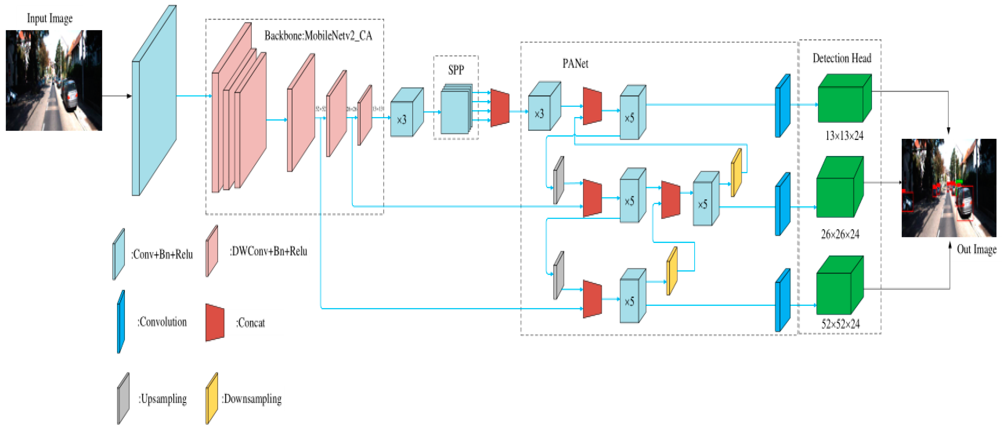
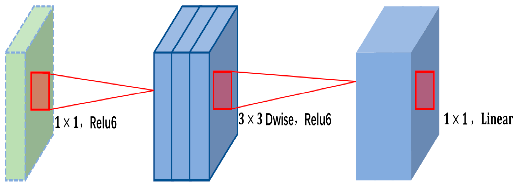
26] dataset using Mobilenetv2 after embedding coordinate attention (CA) as the backbone of the entire network. In this paper, experiments were conducted on the KITTI dataset. The concrete process is as follows: the Adam [27] optimizer was used to train the network on the training set. During the first 50 epochs, the training of the backbone network was frozen, and only the model was slightly adjusted. The feature extraction network did not change. The initial learning rate was set to 10−3 and the batch size was set to 16. After 50 epochs, the network backbone training was unfrozen. After the feature extraction network changed, all the parameters of the network would then change. The initial learning rate was 10−4 and the batch size was 8. The multiplication factor and weight attenuation of the updated learning rate were 0.94 and 0.0005, respectively. The IoU threshold was set to 0.5. The mean average precision (mAP) of each class was evaluated on the validation set.
The loss function is an important index to evaluate the training effect of the network, and the corresponding loss function in this paper consisted of three parts: the location loss function ( L o s s c I o u ), the confidence loss function ( L o s s c o n ) and the class loss function ( L o s s c l s ). The total loss function was L o s s = r 1 L o s s l o c + r 2 L o s s c o n + r 3 L o s s c l s , where r 1 represents the localization loss function coefficient, r 2 represents the confidence loss function coefficient and r 3 represents the category loss function coefficient. r 1 = 0.05 , r 2 = i n p u t [ 0 ] × i n p u t [ 1 ] 416 2 , r 3 = 1 × n u m c l a s s e s 80 . In different datasets, the values of r 1 and r 2 will change according to the specific situation. Additionally, the loss function of confidence and class adopted the cross-entropy loss function, and the loss function of location adopted CIoU [28] loss. CIoU loss function makes the object box regression more stable, and it does not face problems such as scattering during IoU training, is sensitive to scale transformation and converges faster than IoU loss function. Then, for the bounding box localization loss L o s s l o c , the IoU loss function needs to be replaced by the CIoU loss function, which can be expressed as:
{ α = ν 1 I o U + ν ν = 4 π 2 ( arctan ω g t h g t arctan ω h ) 2
where ω and ω g t and h and h g t , respectively, represent the width and height of the prediction frame and the true frame. The loss function L o s s l o c of the corresponding CIoU can be expressed as:
L o s s l o c = 1 C I o U = 1 I o U + ρ 2 ( b , b g t ) c 2 + α ν
The prediction confidence loss function L o s s c o n is measured by the cross-entropy loss function, which can be expressed as:
L o s s c o n = i = 0 s 2 j = 0 B I i , j o b j [ C ^ i j log ( C i j ) + ( 1 C ^ i j ) log ( 1 C i j ) ] λ n o o b j i = 0 s 2 j = 0 B I i , j n o o b j [ C ^ i j log ( C i j ) + ( 1 C ^ i j ) log ( 1 C i j ) ]
where s 2 is the number of divided grids and B is the number of prior frames contained in each grid. I i , j o b j and I i , j n o o b j indicate whether the j -th prior frame of the i -th grid contains an object and whether it is set to 1 or 0. λ n o o b j is the confidence error weight of the prior frame without objects; it has an extremely small value because positive samples and negative samples in prior frame are extremely unbalanced (there are very few prior frames with objects).
The class loss L o s s c l s was used to measure the class error between the prediction frame and the true frame, and was measured by the cross-entropy loss function, which can be expressed as:
L o s s c l s = 0 s 2 I i , j o b j c c l a s s e s [ P ^ i j log ( P i j ) + ( 1 P ^ i j ) log ( 1 P i j ) ]
where P and P ^ represent the class probabilities of the prediction frame and the true frame, respectively.

3.3. Evaluation Indexes

General object detection evaluation indexes were adopted: precision (P), recall rate (R), average precision (AP) and mean average precision (mAP), represented by:
P = TP TP + FP
R = TP TP + FN
mAP = i = 1 k AP i k
AP = 0 1 P ( R ) d R
where true positive (TP) represents the true case, false positive (FP) represents the false positive case, false negative (FB) represents the false negative case and k is the category.
In this paper, the recall R was divided into six points (0, 0.2, 0.4, ..., 1.0), and the precision P under each recall was obtained according to the calculation of PASCAL VOC [22]. Then, the P–R curve was obtained, and the area enclosed by the P–R curve and the coordinate axis denotes the AP value. For each class, the AP was calculated in the above manner, and the average of the AP for all classes was the mAP.

3.4. Analysis of Experimental Results

To verify the effectiveness of using the Mosaic image enhancement method and adding the coordinate attention (CA) mechanism to Mobilenetv2—the lightweight backbone feature extraction network—ablation experiments were designed for different modules. Ablation experiments were performed on two different datasets: KITTI and VOC.
Performing ablation experiments of the same module using a variety of different datasets can effectively verify whether each module can adapt to different task requirements in different scene datasets, and verify the actual contribution of each module to the network.
√ in Table 3 represents the participation of the module. This module is represented in Table 3. A denotes use of the Mobilenetv2 backbone network, B is with the addition of the coordinate attention (CA) mechanism to the backbone network, and C is with the addition of the Mosaic image enhancement to the data pre-processing stage. To verify that using the Mosaic image enhancement method and a lightweight backbone network incorporating a coordinated attention (CA) mechanism can improve the precision of network detection, a comparative experiment was designed.
Networks with the network backbone Mobilenetv1, networks with the network backbone Mobilenetv2, networks with a coordinated attention (CA) mechanism added to backbone Mobilenetv2 and networks with a coordinated attention (CA) mechanism added to backbone Mobilenetv2 using Mosaic image enhancement were trained separately and evaluated on two different datasets: KITTI and VOC. √ in 
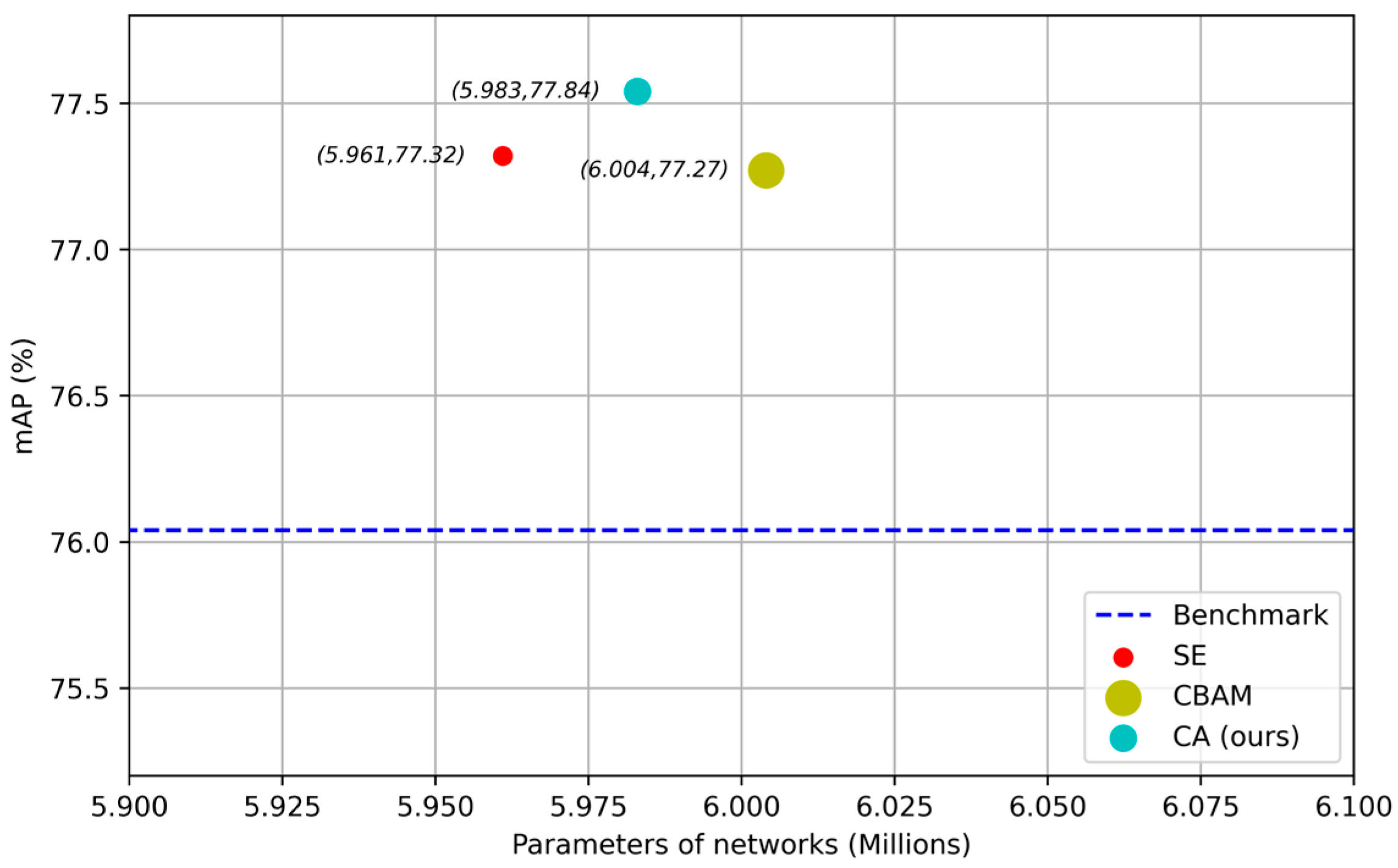
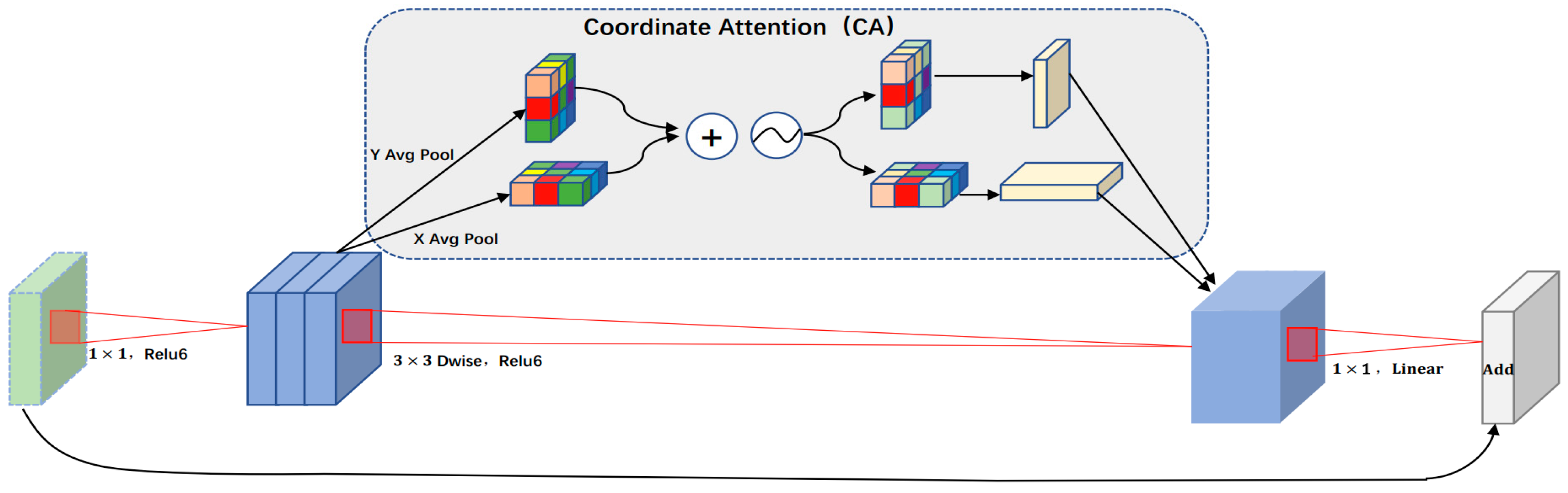
Table 3 represents the participation of this module. By using Mobilenetv2 as the backbone network, compared with the Mobilenetv1 backbone network, the accuracy improved by 2.7% on the KITTI dataset and 0.4% on the VOC dataset, but the detection speed was almost unchanged. Mobilenetv2 is shown to be an efficient and lightweight backbone network. After adding the attention mechanism CA to Mobilenetv2, the network considered both the relationship between the channels and the location information, which enhances the network’s sensitivity to direction and location information, strengthens the extraction of important features, and improves the network’s learning ability. The network accuracy was further improved—by 0.23% on the KITTI dataset and by 1% on the VOC dataset—proving the contribution of CA. After using the Mosaic image enhancement method, the network can detect objects outside the normal context, making the feature extraction of various objects more complete and continuous, allowing the attainment of more abundant image features. The detection accuracy was further improved on the KITTI dataset by 0.28%. On the VOC dataset, the detection accuracy was further improved by 0.31%, proving the contribution of Mosaic image enhancement. Compared with the original network, using Mobilenetv1 as the backbone, the detection accuracy on the KITTI dataset was increased by 3.21%, and the detection accuracy on the VOC dataset increased by 1.71%, which improved the overall generalization performance of the network.
There are many kinds of current object detection networks. To verify the effectiveness of the networks in this paper, a variety of object detection networks were selected for experimental comparison on the KITTI dataset. Faster R-CNN [3], SSD [4], and YOLOv3 [5], YOLOv4 [21], YOLOv5-l [29] and YOLOv4-tiny [
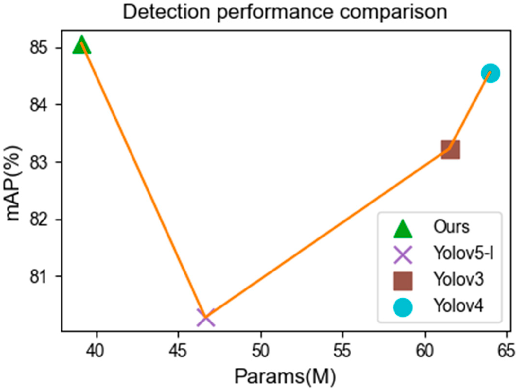
30] algorithms were selected to be trained on the KITTI dataset and compared with this detection network on the test set, focusing on average class accuracy, the number of model parameters, and detection speed.
The parameters in Table 4 refer to the number of parameters of the network, and FPS refers to the number of images processed by the network each second, which can be used to characterize the network’s detection speed performance. As can be seen in Table 4, compared with the Faster R-CNN algorithm, the detection speed of this paper was 3.1 times faster, the detection accuracy of the car improved by 15.14%, the detection accuracy of pedestrians improved by 18.71%, the detection accuracy of cyclists improved by 22.52% and the average detection accuracy (mAP) improved by 18.79%. However, the number of participants significantly decreased by 28.8%. Compared with the SSD algorithm, although the detection speed of this paper’s algorithm was reduced, the detection accuracy for cars improved by 9.57%, for pedestrians by 28.07%, for cyclists by 23.22% and the average detection accuracy (mAP) improved by 20.23% for the same number of model parameters. Compared with the YOLOv3 algorithm, the detection speed is slightly slower, the detection precision of cars is slightly higher, the detection precision of pedestrians improved by 2.73%, the detection precision of cyclists improved by 2.75%, the average detection precision (mAP) of this paper increased by 1.84% and the number of participants was only 63.8% of the YOLOv3 algorithm’s total number of participants. The network performance was better than that of the YOLOv3 algorithm. The network performance of this method was better than that of YOLOv3. Compared with YOLOv4, our algorithm improved by 0.67% in car detection accuracy, with almost the same level of accuracy as when detecting pedestrians. Additionally, an improvement of 1.05% was obtained in the detection accuracy of cyclists, and 0.51% in the average detection accuracy. Compared with YOLOv5, our algorithm improved by 6.23% in the detection accuracy of cars, 2.97% in the detection accuracy of pedestrians, 5.15% in the detection accuracy of cyclists and 4.79% in average detection accuracy. Compared with YOLOv4-tiny, our algorithm improved the average detection accuracy by 24.32%. We focused more on high detection accuracy than on increasing the detection speed. Taken together, the number of network parameters was significantly reduced in this paper, achieving the goal of excellent detection precision with a lightweight network.
In autonomous driving scenarios, cars, pedestrians and cyclists are the most common detection objects, and it is important to achieve high precision detection on the basis of real-time detection. During object detection, the real-time detection requirement is satisfied when the number of images per second that are processed by the network is more than 30 FPS. Therefore, the requirement of real-time detection can be met. Table 4 shows that that the Faster R-CNN network does not meet the requirements of real-time detection, and the SSD network, although it achieved a faster detection speed, has a detection accuracy that is too low to meet the requirements of high-precision detection. Both the YOLOv3 network and the MobileNetv2_CA network in this paper can achieve real-time and high-precision detection. Therefore, the detection precision of the two networks are further compared in Table 5, using the KITTI validation set and three different evaluation criteria. It can be seen that, under the three different criteria, the proposed network has a 2.25%, 1.38% and 0.9% higher detection precision than the YOLOv3 in the car class. The precision of pedestrian detection is 8.8%, 7.65% and 0.8% higher than that of YOLOv3, respectively. The detection precision of cyclists is 0.95%, 0.53% and 0.88% higher than that of YOLOv3, respectively. In conclusion, the detection precision of all the networks in this paper is better than that of the YOLOv3 network, and the number of parameters is only 63.58% of that of the YOLOv3 network. Although the FPS is slightly lower than that of the YOLOv3 network, because the Coordinate Attention (CA) mechanism added in this paper takes time to extract rich features, the detection precision of this network is higher if the real-time detection FPS is greater than 30 FPS. A scheme combining a better detection speed and precision was achieved under the premise of ensuring a lightweight network.
In the relevant traffic scenes of the autonomous driving KITTI dataset, vehicles (car) and pedestrians (pedestrian) are the main detection objects, and the pedestrian (pedestrian) class is a small target compared to the vehicle (car). During the data pre-processing stage, the Mosaic data enhancement method is used, and the network enhances the sensitivity of the network, allowing for it to detect small targets through pre-processing methods such as scaling the target image. When the backbone feature extraction network extracts relevant features, it coordinates the attention mechanism. In this algorithm, according to the uneven distribution of the large and small objects in the image, the information between the channels can be cooperatively processed, and more attention is paid to the adaptive extraction of the position information of objects of different sizes compared with the comparison algorithm without the attention mechanism. This increases the location information extraction of small targets. Therefore, compared with the vehicle (car) class detection accuracy, there were 2.25%, 1.38% and 0.9% gains under the different standards. In the pedestrian (pedestrian) class detection accuracy, higher gains of 8.8%, 7.65% and 0.8% were obtained under different standards. To show the difference in time taken by different layers in specific detection tasks in more detail, this paper split and refined different parts of the model for time series analysis.
Experiments on a single dataset may not be very convincing, and more datasets need to be tested and verified to draw better conclusions. Therefore, we selected several categories that are more common in autonomous driving scenarios for comparison. The results show that, on the Pascal Voc2007 + 2012 dataset, as show in Table 6, our method improved the bus category by 0.29% compared to Faster R-CNN. The results were also 0.76% higher than SSD, 1.66% higher than Yolov3, 2.22% higher than Faster R-CNN in the motorbike category, 1.62% higher than SSD and 2.07% higher than Yolov3. In the person category, compared with Faster R-CNN, accuracy improved by 0.06%—by 5.31% compared with SSD and by 0.1% compared with Yolov3. Compared with Faster R-CNN on mAP, accuracy improved by 1.15%, was 3% higher than SSD and was 2.07% higher than Yolov3. Compared with YOLOv4, our algorithm showed little difference in terms of detection accuracy and detection speed, but the number of parameters in our model was almost half that of YOLOv4. Compared with YOLOv5, our algorithm improved the average detection accuracy by 6.26%. Compared with YOLOv4-tiny, our algorithm improved the average detection accuracy by 4.89%.
As shown in Table 7, we also explored the effect of using different original image scaling ratios and width-to-height distortion ratios on the detection accuracy, and finally determined our parameter range to achieve the highest detection accuracy.

3.5. Network Detection Effect

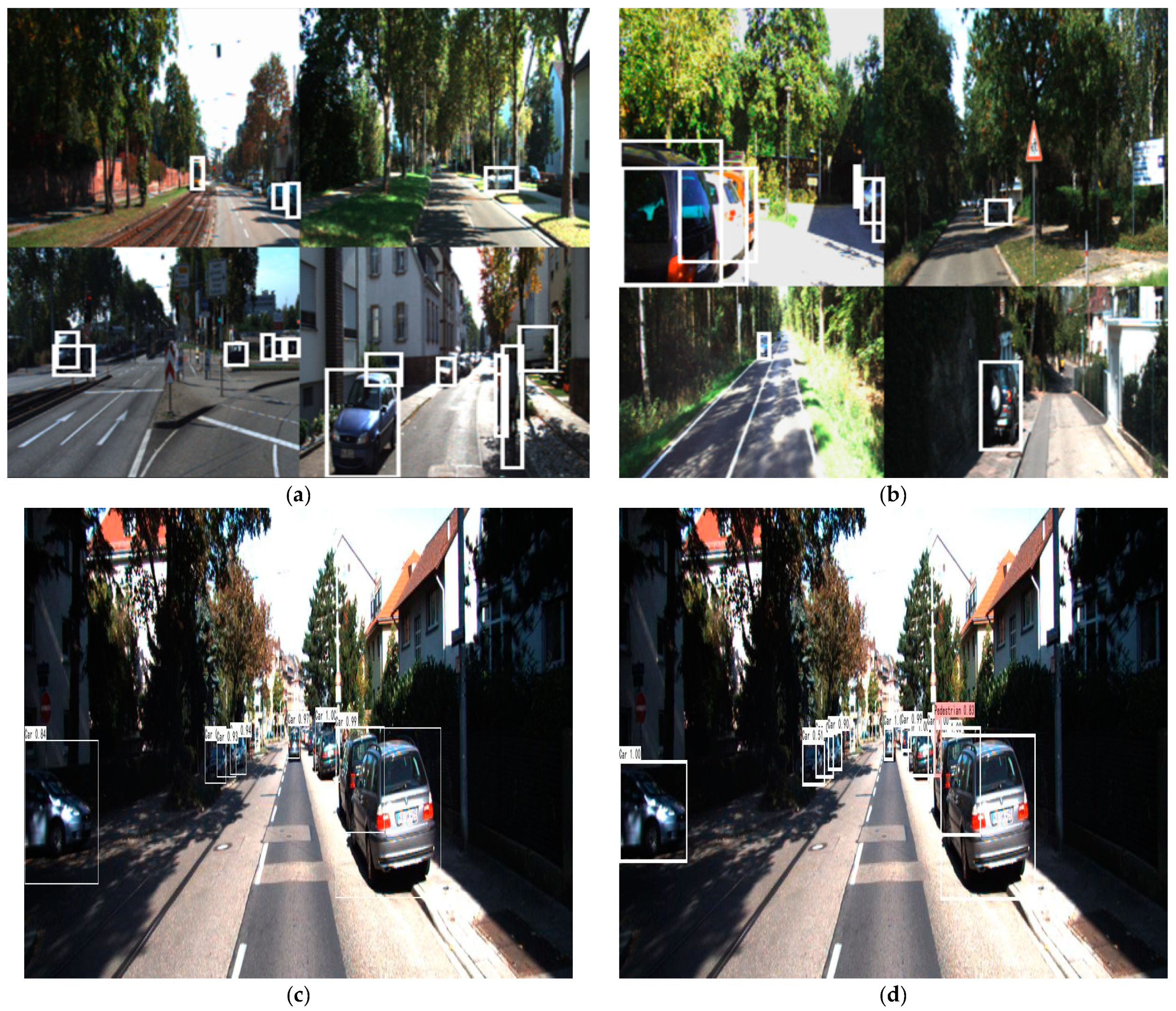
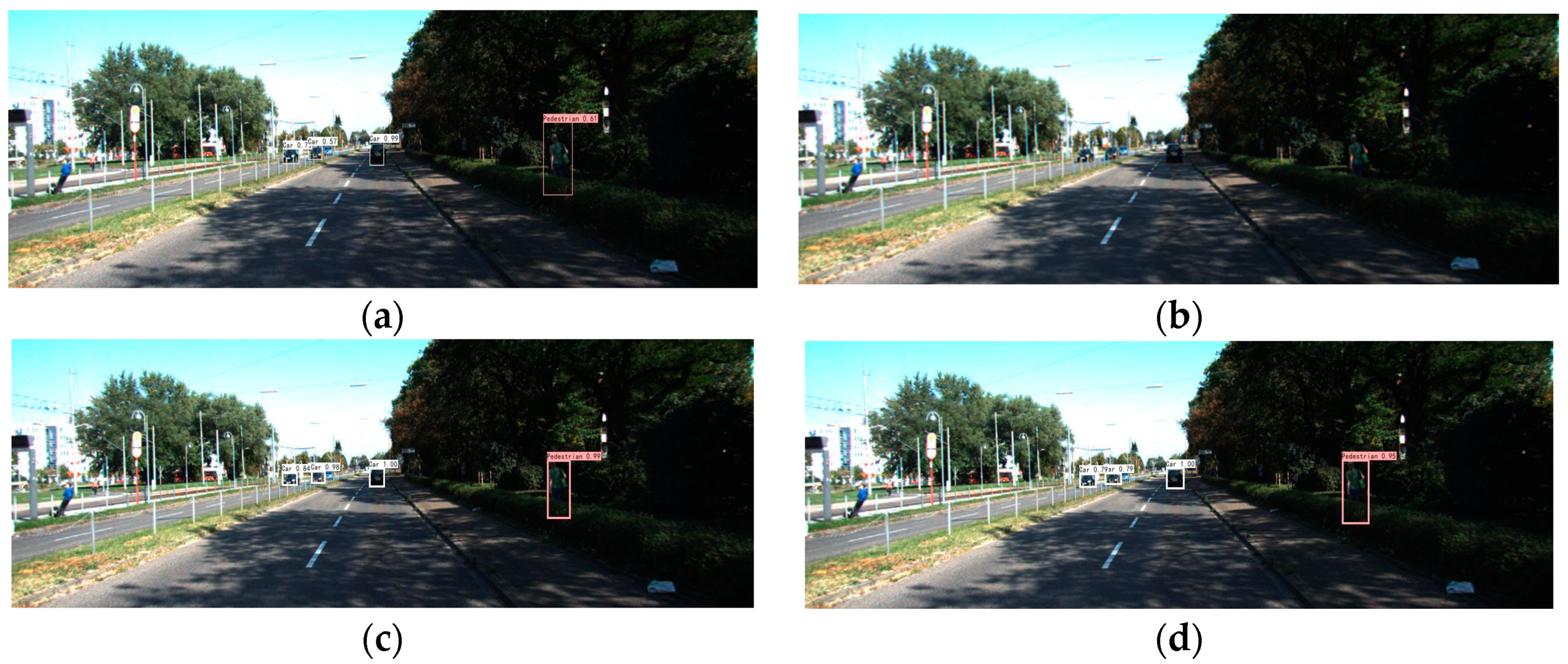
To intuitively reflect the detection performance of this model, some pictures with a complex image environment that are difficult to distinguish were selected from the KITTI test set for detection. Figure 8 shows the small object scene. Figure 8a shows the Faster R-CNN detection effect. Although it can achieve more accurate object detection, its detection speed is too slow to meet the real-time detection requirements. Figure 8b shows the SSD detection effect, which shows a more serious leakage phenomenon and does not detect any object. Figure 8c shows the detection effect of YOLOv3 with some missed detections. Figure 8d shows the detection effect of the network in this paper, which can more comprehensively and accurately detect the emerged objects. 
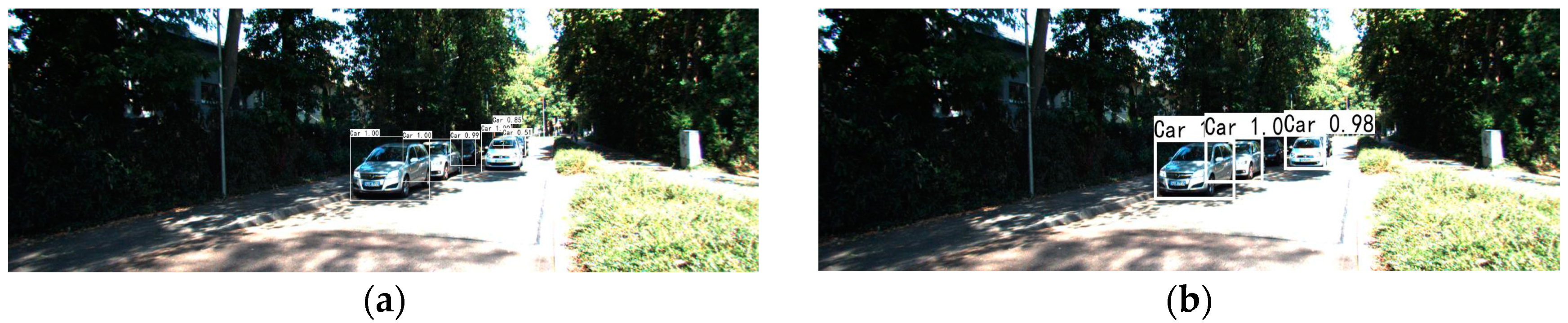
Figure 9 shows low-light scenes. Figure 9a shows the Faster R-CNN detection effect in low-light intensity scenes, while the vehicle located on the right side of the scene in the low-light environment was missed. Figure 9b shows the SSD detection effect, where both the vehicle on the right side in the low-light environment and the vehicle on the left side, which belonged to a smaller target, were missed. 
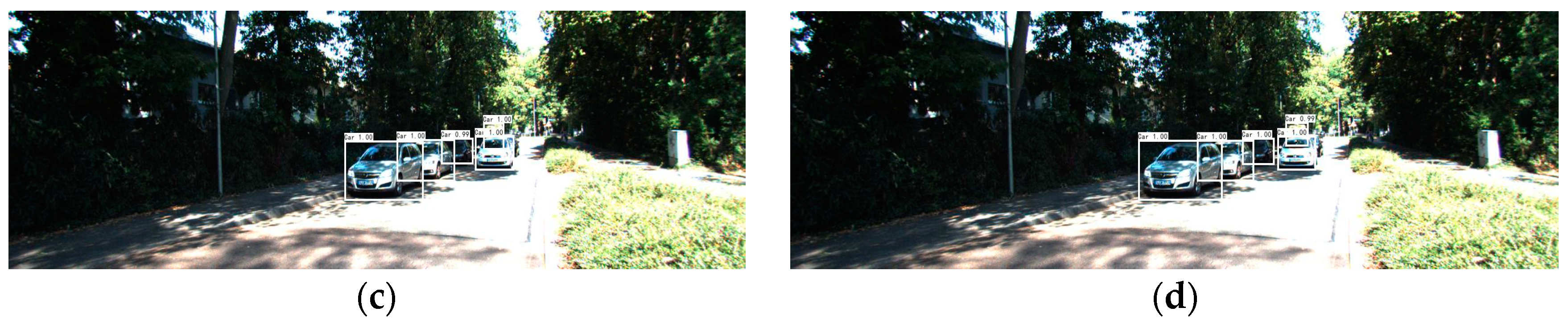
Figure 9c shows the detection effect of YOLOv3, which contains a high number of parameters despite achieving real-time detection of the target. Figure 9d shows the detection effect of the network in this paper, which can precisely detect both vehicles in the low-light environment as well as vehicles belonging to smaller objects. 
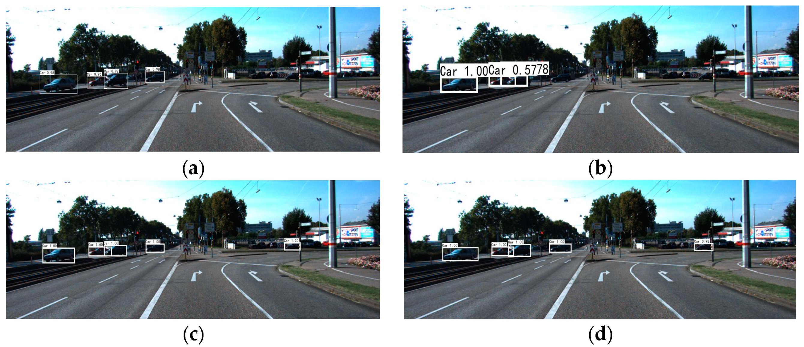
Figure 10 shows a complex scene containing small objects, occlusion, high light intensity and low light intensity, etc. Figure 10a shows the Faster R-CNN detection effect. Although it can achieve a more accurate target detection, its detection speed is too slow to meet the real-time detection requirements. Figure 10b shows the effect of SSD detection, and the detection phenomenon was missed for vehicles at a low light intensity and rear-obstructed vehicles. Figure 10c shows the detection effect of YOLOv3, which can better detect the object, and 
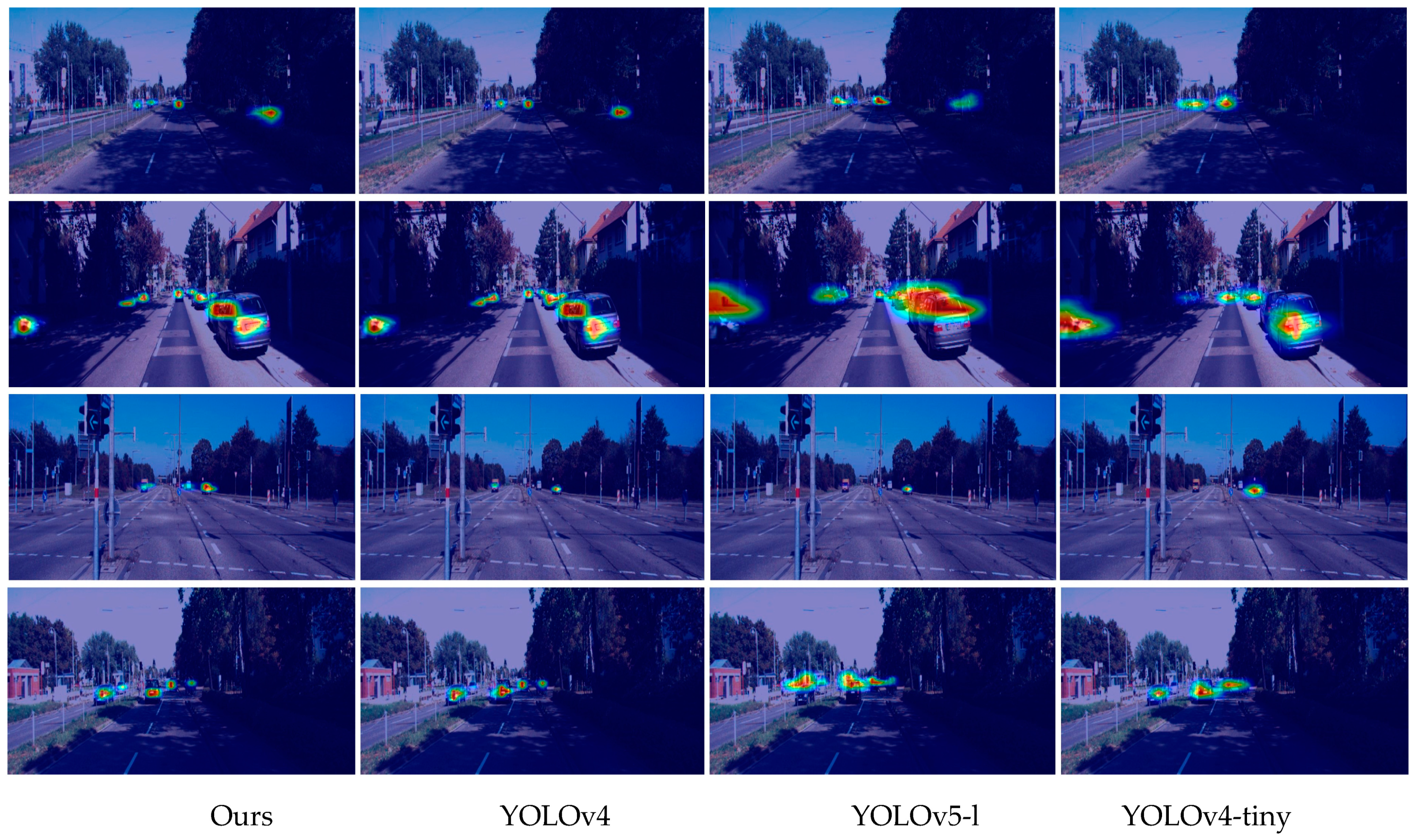
Figure 10d shows the detection effect of this network, which can correctly and simultaneously detect all the objects at a low light intensity, high light intensity and obscured objects. In summary, the network used in this paper can quickly and accurately complete detection tasks in different scenarios; therefore, the network proposed in this paper is a real-time object detection network with a light weight and high precision. To more clearly show the difference in the detection results of different models for targets in different KITTI dataset scenes, we visualized the final detection results of different models in a heat map. The first column in Figure 11 shows the detection results of our work. It is clear that our model can accurately locate and detect hard-to-differentiate persons with the right shade in the first scenario, hard-to-differentiate two-vehicle targets with the left shade in the second scenario, and the smaller vehicle in the opposite lane and the vehicle target in the same direction in the third scenario. These scenarios took place in a poor lighting environment. In the fourth scenario, the smaller vehicle in the opposite lane and the vehicle in the same direction were accurately located and detected. This demonstrates the better robustness of our model compared toYOLOv4, YOLOv5, and YOLOv4-tiny in handling autonomous driving scenarios.
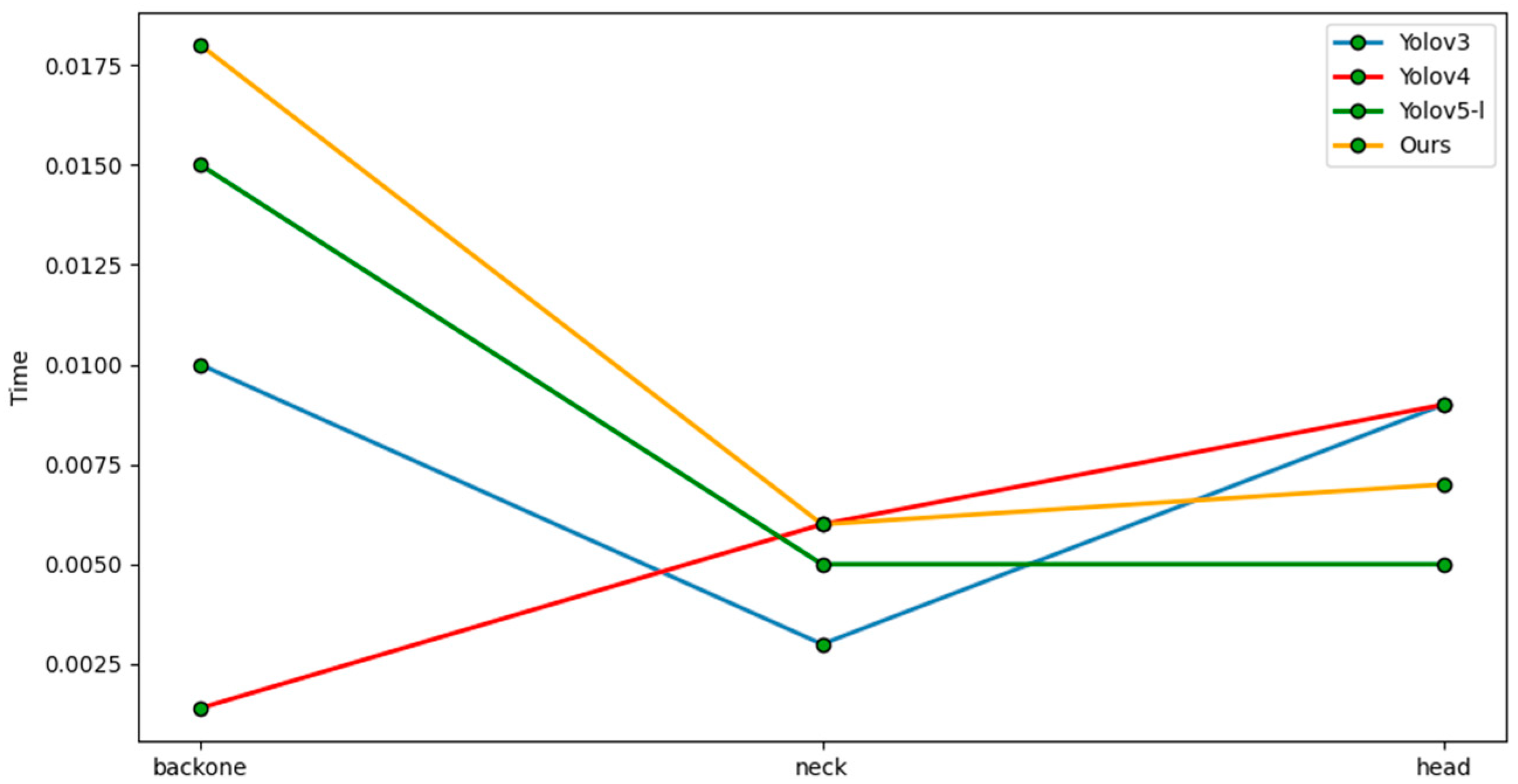
After comprehensively weighing the detection accuracy and the number of network parameters, our method could achieve real-time detection. A runtime comparison of each part of various detectors is shown in Figure 11. To show the time-consuming differences between different layers during specific detection tasks in more detail, this paper split and refined the different parts of the model to analyze the runtime. Our model mainly uses the attention mechanism to extract backbone features. This is slightly more time-consuming, but real-time detection is still possible.
At the same time, in order to clearly show the superiority of our algorithm model in capturing small objects or occluded objects, we drew the heat map shown in Figure 12 below, from which it can be seen that our algorithm model uses the attention mechanism in the process of network training and learning, strengthens some signals in the heat map and suppresses other parts, making the network extraction features more accurate.

4. Discussion

This paper studies and explores a lightweight object detection network, which reduces the complexity of the object detection network and can achieve efficient and accurate object detection in autonomous driving embedded platform devices. We propose a method of feature extraction, using an improved lightweight neural network as the backbone. First, the Mosaic image enhancement method was used, and an efficient lightweight backbone was used. These were combined with a coordinated attention mechanism to guide the initial feature extraction of the entire network, and then combined with a multi-scale feature fusion network to fuse image features with location information and semantic information to obtain richer image features. Finally, a multi-scale predictor was used for prediction to obtain the detection results. In this article, our related experiments show that our method has obvious advantages in terms of network parameters over the comparison network, which obtained only 39.1 M, and is even better in terms of robustness. Whether referring to the average precision of 85.07% on the KITTI dataset or the detection accuracy of 81.43% on the Voc2007 + 2012 dataset, our method achieved robustness. Regarding the detection accuracy in the automatic driving scene, which requires high detection accuracy, achieving a robust accuracy performance is of great significance. Our method also met the speed requirements of automatic driving target detection in terms of delay, reaching a 31.84 FPS detection speed performance. In terms of comprehensive computing resources, robustness and real-time performance, our method achieved the best performance coupling. As an efficient target detection algorithm, the lightweight neural network can also be applied to some other fields. For example, in the field of smart cities, our algorithm can be deployed in smart traffic lights. It can also be used to monitor the real-time flow of people and vehicles at an intersection, and intelligently change the duration of traffic lights according to the flow size.

5. Conclusions

The purpose of this paper was to explore a lightweight and efficient target detection algorithm that can be efficiently deployed on smart cars. Target detection is different when not using simple scenes. Our method was used in complex traffic scenes. We used an efficient coordination mechanism for lightweight backbone network feature extraction and fusion, focusing on optimizing pre-processing methods and multi-scale feature fusion networks. In this way, our work achieved a better performance than previous work in autonomous driving scenarios. It realized the fast and accurate detection of targets in various traffic scenarios and has great application potential in actual autonomous driving scenarios. In future work, our focus will be on further optimizing our detection speed. The next step is to continue to optimize the network model to improve the detection speed and accuracy, allowing for the network to adapt to more complex traffic scenes and achieve a robust detection in actual complex traffic scenes.

Author Contributions

P.S.: Conceptualization, Methodology, Investigation, Funding acquisition. L.L.: Software, Data Curation, Writing—Original Draft. H.Q.: Visualization, Validation. A.Y.: Writing—Review and Editing, Supervision. All authors have read and agreed to the published version of the manuscript.

Funding

This work was supported by the financial support of the key research and development projects of Anhui (202104a05020003), Anhui development and reform commission support of the R&D and innovation project ([2020]479).

Institutional Review Board Statement

Not applicable.

Informed Consent Statement

Not applicable.

Data Availability Statement

The data used in this study are available upon request.

Conflicts of Interest

The authors declare no conflict of interest.

References

  1. Dalal, N.; Triggs, B. Histograms of oriented gradients for human detection. In Proceedings of the IEEE Conference on Computer Vision and Pattern Recognition, San Diego, CA, USA, 20–26 June 2005; IEEE Computer Society: San Diego, CA, USA, 2005; pp. 886–893. [Google Scholar]
  2. Lowe, D.G. Distinctive image features from scale-invariant key points. Int. J. Comput. Vision. 2004, 60, 91–110. [Google Scholar] [CrossRef]
  3. Ren, S.; He, K.; Girshick, R.; Sun, J. Faster r-cnn: Towards real-time object detection with region proposal networks. Adv. Neural Inf. Process. Syst. 2015, 28, 2969239–2969250. [Google Scholar] [CrossRef] [PubMed] [Green Version]
  4. Liu, W.; Anguelov, D.; Erhan, D.; Szegedy, C.; Reed, S.; Fu, C.Y.; Berg, A.C. Ssd: Single shot multibox detector. In Proceedings of the European Conference on Computer Vision; Springer: Cham, Switzerland, 2016; pp. 21–37. [Google Scholar]
  5. Redmon, J.; Farhadi, A. Yolov3: An incremental improvement. arXiv 2018, arXiv:1804.02767. [Google Scholar]
  6. Ge, Z.; Liu, S.; Wang, F.; Li, Z.; Sun, J. Yolox: Exceeding yolo series in 2021. arXiv 2021, arXiv:2107.08430. [Google Scholar]
  7. Xu, S.; Wang, X.; Lv, W.; Chang, Q.; Cui, C.; Deng, K.; Wang, G.; Dang, Q.; Wei, S.; Du, Y.; et al. PP-YOLOE: An evolved version of YOLO. arXiv 2022, arXiv:2203.16250. [Google Scholar]
  8. Liu, Z.; Hu, H.; Lin, Y.; Yao, Z.; Xie, Z.; Wei, Y.; Ning, J.; Cao, Y.; Zhang, Z.; Dong, L.; et al. Swin transformer v2: Scaling up capacity and resolution. In Proceedings of the IEEE/CVF Conference on Computer Vision and Pattern Recognition, New Orleans, LA, USA, 18–24 June 2022; pp. 12009–12019. [Google Scholar]
  9. Han, S.; Mao, H.; Dally, W.J. Deep compression: Compressing deep neural networks with pruning, trained quantization and huffman coding. arXiv 2015, arXiv:1510.00149. [Google Scholar]
  10. Li, H.; Kadav, A.; Durdanovic, I.; Samet, H.; Graf, H.P. Pruning filters for efficient convnets. arXiv 2016, arXiv:1608.08710. [Google Scholar]
  11. Rastegari, M.; Ordonez, V.; Redmon, J.; Farhadi, A. Xnor-net: Imagenet classification using binary convolutional neural networks. In Proceedings of the European Conference on Computer Vision; Springer: Cham, Switzerland, 2016; pp. 525–542. [Google Scholar]
  12. Hinton, G.; Vinyals, O.; Dean, J. Distilling the knowledge in a neural network. arXiv 2015, arXiv:1503.02531. [Google Scholar]
  13. Han, K.; Wang, Y.; Tian, Q.; Guo, J.; Xu, C.; Xu, C. Ghostnet: More features from cheap operations. In Proceedings of the IEEE/CVF Conference on Computer Vision and Pattern Recognition, Seattle, WA, USA, 13–19 June 2020; pp. 1580–1589. [Google Scholar]
  14. Iandola, F.N.; Han, S.; Moskewicz, M.W.; Ashraf, K.; Dally, W.J.; Keutzer, K. SqueezeNet: AlexNet-level precision with 50x fewer parameters and <0.5 MB model size. arXiv 2016, arXiv:1602.07360. [Google Scholar]
  15. Zhang, X.; Zhou, X.; Lin, M.; Sun, J. Shufflenet: An extremely efficient convolutional neural network for mobile devices. In Proceedings of the IEEE Conference on Computer Vision and Pattern Recognition, Salt Lake City, UT, USA, 18–23 June 2018; pp. 6848–6856. [Google Scholar]
  16. Howard, A.G.; Zhu, M.; Chen, B.; Kalenichenko, D.; Wang, W.; Weyand, T.; Andreetto, M.; Adam, H. Mobilenets: Efficient convolutional neural networks for mobile vision applications. arXiv 2017, arXiv:1704.04861. [Google Scholar]
  17. Sandler, M.; Howard, A.; Zhu, M.; Zhmoginov, A.; Chen, L.C. Mobilenetv2: Inverted residuals and linear bottlenecks. In Proceedings of the IEEE Conference on Computer Vision and Pattern Recognition, Salt Lake City, UT, USA, 18–23 June 2018; pp. 4510–4520. [Google Scholar]
  18. Hou, Q.; Zhou, D.; Feng, J. Coordinate attention for efficient mobile network design. In Proceedings of the IEEE/CVF Conference on Computer Vision and Pattern Recognition, Nashville, TN, USA, 20–25 June 2021; pp. 13713–13722. [Google Scholar]
  19. He, K.; Zhang, X.; Ren, S.; Sun, J. Spatial pyramid pooling in deepwise convolutional networks for visual recognition. IEEE Trans. Pattern Anal. Mach. Intell. 2015, 37, 1904–1916. [Google Scholar] [CrossRef] [PubMed] [Green Version]
  20. Liu, S.; Qi, L.; Qin, H.; Shi, J.; Jia, J. Path aggregation network for instance segmentation. In Proceedings of the IEEE Conference on Computer Vision and Pattern Recognition, Salt Lake City, UT, USA, 18 June–23 June 2018; IEEE Computer Society: Salt Lake City, UT, USA, 2018; pp. 8759–8768. [Google Scholar]
  21. Bochkovskiy, A.; Wang, C.Y.; Liao HY, M. Yolov4: Optimal speed and precision of object detection. arXiv 2020, arXiv:2004.10934. [Google Scholar]
  22. Everingham, M.; Eslami, S.A.; Van Gool, L.; Williams, C.K.; Winn, J.; Zisserman, A. The pascal visual object classes challenge: A retrospective. Int. J. Comput. Vis. 2015, 111, 98–136. [Google Scholar] [CrossRef]
  23. Hu, J.; Shen, L.; Sun, G. Squeeze-and-excitation networks. In Proceedings of the IEEE Conference on Computer Vision and Pattern Recognition, Salt Lake City, UT, USA, 18–23 June 2018; pp. 7132–7141. [Google Scholar]
  24. Woo, S.; Park, J.; Lee, J.Y.; Kweon, I.S. Cbam: Convolutional block attention module. In Proceedings of the European Conference on Computer Vision (ECCV), Munich, Germany, 8–14 September 2018; pp. 3–19. [Google Scholar]
  25. Geiger, A.; Lenz, P.; Urtasun, R. Are we ready for autonomous driving? The kitti vision benchmark suite. In Proceedings of the 2012 IEEE Conference on Computer Vision and Pattern Recognition; IEEE: Manhattan, NY, USA, 2012; pp. 3354–3361. [Google Scholar]
  26. Deng, J.; Dong, W.; Socher, R.; Li, L.J.; Li, K.; Fei-Fei, L. Imagenet: A large-scale hierarchical image database. In Proceedings of the 2009 IEEE Conference on Computer Vision and Pattern Recognition, Miami, FL, USA, 20–25 June 2009; IEEE: Manhattan, NY, USA, 2009; pp. 248–255. [Google Scholar]
  27. Kingma, D.P.; Ba, J. Adam: A method for stochastic optimization. arXiv 2014, arXiv:1412.6980. [Google Scholar]
  28. Zheng, Z.; Wang, P.; Ren, D.; Liu, W.; Ye, R.; Hu, Q.; Zuo, W. Enhancing geometric factors in model learning and inference for object detection and instance segmentation. IEEE Trans. Cybern. 2021, 52, 8574–8586. [Google Scholar] [CrossRef] [PubMed]
  29. Glenn Jocher. Yolov5. 2021. 1, 2, 3, 5, 6. Available online: https://github.com/ultralytics/yolov5 (accessed on 5 February 2023).
  30. Wang, C.Y.; Bochkovskiy, A.; Liao HY, M. Scaled-yolov4: Scaling cross stage partial network. In Proceedings of the IEEE/CVF Conference on Computer Vision and Pattern Recognition, Nashville, TN, USA, 20–25 June 2021; pp. 13029–13038. [Google Scholar]
Figure 1. Advanced model performance comparison chart.
Technologies 11 00047 g001
Figure 2. The input image is passed through the backbone feature extraction network to the multi-scale pooling layer, multi-scale fusion is performed, and, finally, the detection result is output.
Technologies 11 00047 g002
Figure 3. Test effect of Mosaic image enhancement method in different scenarios. (a) Small object scenes; (b) obscured objects and objects in low-light state scenes; (c) with the Mosaic data enhancement detection effect diagram closed; (d) with the Mosaic data enhancement detection effect diagram open.
Technologies 11 00047 g003
Figure 4. Linear Bottleneck Block.
Technologies 11 00047 g004
Figure 5. Performance comparison of different attention mechanisms.
Technologies 11 00047 g005
Figure 6. The overall structure diagram after embedding the coordinated attention mechanism, called the Inverted Residuals_CA Block.
Technologies 11 00047 g006
Figure 7. Multi-scale feature fusion and prediction were used to fuse location and semantic information at different scales.
Technologies 11 00047 g007
Figure 8. Small target scenes. (a) Faster R-CNN detection effect, (b) SSD detection effect, (c) YOLOv3 detection effect, (d) MobileNetv2_CA detection effect.
Technologies 11 00047 g008
Figure 9. Low-light scenes. (a) Faster R-CNN detection effect, (b) SSD detection effect, (c) YOLOv3 detection effect, (d) MobileNetv2_CA detection effect.
Technologies 11 00047 g009
Figure 10. Complex scenes. (a) Faster R-CNN detection effect, (b) SSD detection effect, (c) YOLOv3 detection effect, (d) MobileNetv2_CA.
Technologies 11 00047 g010aTechnologies 11 00047 g010b
Figure 11. Time-consuming difference diagram of different modules.
Technologies 11 00047 g011
Figure 12. Heat map visualization results of detection results for different models in different scenarios in the KITTI dataset. The first column shows our results, the second column shows the results for YOLOv4, the third column shows the results for YOLOv5-l and the fourth column shows the results for YOLOv4-tiny.
Technologies 11 00047 g012
Table 1. Overall structure of Mobilenetv2_CA.
InputOperatortcns
416 2 × 3Conv2d-3212
208 2 × 32Bottleneck11611
208 2 × 16Bottleneck62422
104 2 × 24Bottleneck63232
52 2 × 32Bottleneck66442
26 2 × 64Bottleneck69631
26 2 × 96Bottleneck616032
13 2 × 160Bottleneck632011
13 2 × 320Conv2d1 × 1-128011
7 2 × 1280Avgpool7 × 7--1-
1 × 1 × 1280Conv2d1 × 1-k-
Table 2. Dataset partition details.
ClassNumberCarCyclistPedestrian
train&val673230,00514804277
test7493256147432
ClassNumberCarBusMotorbikePerson
train&val896711,1671329152241,146
test99612012133254528
Table 3. Ablation experiment.
ModelABCmAP (%)Promotion Rate (%)
KITTIMobilenetv1-PANet 81.86/
Mobilenetv2-PANet 84.562.70
Mobilenetv2-CA-PANet 84.792.93
Mobilenetv2-CA-M-PANet85.073.21
VOCMobilenetv1-PANet 79.72/
Mobilenetv2-PANet 80.120.4
Mobilenetv2-CA-PANet 81.121.4
Mobilenetv2-CA-M-PANet81.431.71
Table 4. Performance comparison of different detection networks on KITTI dataset.
Model A P c a r     A P p e d e s t r i a n   A P c y c l i s t   mAP (%)ParametersFPS
Faster R-CNN [3]80.2253.1565.4666.28136.7 M10.33
SSD [4]85.7943.7964.7664.8423.9 M72.36
YOLOv3 [5]95.3469.1385.2383.2361.5 M45.03
YOLOv4 [21]94.6972.0586.9384.5663.95 M34.79
YOLOv5-l [29]89.1368.8982.8380.2846.64 M39.51
YOLOv4-tiny [30]82.1139.8061.1360.758.879 M129.32
MobileNetv2_CA (ours)95.3671.8687.9885.0739.1 M31.84
Table 5. Performance comparison using KITTI validation set (where Easy, Moderate and Hard refer to the precision under easy, moderate and hard standards, respectively).
Average Precision (%)
ModelStandardCarPedestrianCyclist
YOLOv3 [5]Easy83.7268.9789.66
Moderate85.5160.5280.57
Hard77.1659.3380.20
MobileNetv2_CA (ours)Easy85.9777.7790.61
Moderate86.8968.1781.10
Hard78.0660.1381.08
Table 6. Pascal Voc2007 + 2012 dataset detection performance.
Model A P c a r A P b u s A P m o t o r b i k e A P p e r s o n mAP (%)
Faster R-CNN [3]88.7186.6984.8185.3780.28
SSD [4]88.3786.2285.4180.1278.43
YOLOv3 [5]91.5485.3284.9685.3379.36
YOLOv4 [21]90.6192.8982.7687.2881.05
YOLOv5-l [29]88.6390.5476.4387.9675.17
YOLOv4-tiny [30]90.7683.4284.0384.3476.54
MobileNetv2_CA (ours)91.1186.9887.0385.4381.43
Table 7. Effect of different original image scaling ratios and width-to-height distortion ratios on detection accuracy.
rmAP (%)
r184.29
r284.37
Ours85.07
Disclaimer/Publisher’s Note: The statements, opinions and data contained in all publications are solely those of the individual author(s) and contributor(s) and not of MDPI and/or the editor(s). MDPI and/or the editor(s) disclaim responsibility for any injury to people or property resulting from any ideas, methods, instructions or products referred to in the content.

