GDAL and PROJ Libraries Integrated with GRASS GIS for Terrain Modelling of the Georeferenced Raster Image

Abstract

Libraries with pre-written codes optimize the workflow in cartography and reduce labour intensive data processing by iteratively applying scripts to implementing mapping tasks. Most existing Geographic Information System (GIS) approaches are based on traditional software with a graphical user’s interface which significantly limits their performance. Although plugins are proposed to improve the functionality of many GIS programs, they are usually ad hoc in finding specific mapping solutions, e.g., cartographic projections and data conversion. We address this limitation by applying the principled approach of Geospatial Data Abstraction Library (GDAL), library for conversions between cartographic projections (PROJ) and Geographic Resources Analysis Support System (GRASS) GIS for geospatial data processing and morphometric analysis. This research presents topographic analysis of the dataset using scripting methods which include several tools: (1) GDAL, a translator library for raster and vector geospatial data formats used for converting Earth Global Relief Model (ETOPO1) GeoTIFF in XY Cartesian coordinates into World Geodetic System 1984 (WGS84) by the ‘gdalwarp’ utility; (2) PROJ projection transformation library used for converting ETOPO1 WGS84 grid to cartographic projections (Cassini–Soldner equirectangular, Equal Area Cylindrical, Two-Point Equidistant Azimuthal, and Oblique Mercator); and (3) GRASS GIS by sequential use of the following modules: r.info, d.mon, d.rast, r.colors, d.rast.leg, d.legend, d.northarrow, d.grid, d.text, g.region, and r.contour. The depth frequency was analysed by the module ‘d.histogram’. The proposed approach provided a systematic way for morphometric measuring of topographic data and combine the advantages of the GDAL, PROJ, and GRASS GIS tools that include the informativeness, effectiveness, and representativeness in spatial data processing. The morphometric analysis included the computed slope, aspect, profile, and tangential curvature of the study area. The data analysis revealed the distribution pattern in topographic data: 24% of data with elevations below 400 m, 13% of data with depths −5000 to −6000 m, 4% of depths have values −3000 to −4000 m, the least frequent data (−6000 to 7000 m) <1%, 2% of depths have values −2000 to 3000 m in the basin, while other values are distributed proportionally. Further, by incorporating the generic coordinate transformation software library PROJ, the raster grid was transformed into various cartographic projections to demonstrate distortions in shape and area. Scripting techniques of GRASS GIS are demonstrated for applications in topographic modelling and raster data processing. The GRASS GIS shows the effectiveness for mapping and visualization, compatibility with libraries (GDAL, PROJ), technical flexibility in combining Graphical User Interface (GUI), and command-line data processing. The research contributes to the technical cartographic development.

1. Introduction

1.1. Background

Topographic modelling is a central problem in cartography, land surface modelling, geodesy, and mapping [1]. A basis form of spatial analysis, topographic modelling consists of visualisation of the land surface and plotting contours that reveal variations in elevation and enables landform delineation [2,3]. Tasks such as geomorphic gradients, hydrological modelling, or stream profiling all require topographic analysis. While Geographic Information System (GIS) spatial analysis focuses on complex problems regarding modelling the Earth’s shape [4,5], the technical aspects of spatial data handling consists of various tasks such as data capture [6,7,8], multi-source data formatting and processing [9,10,11], computational analysis and modelling [12,13,14,15], and visualization and mapping [16,17,18].

Maps became a successful form of geospatial data processing since they help exploit the complex phenomena of diverse processes and geographic objects on the Earth’s surface [19]. For instance, features such as elevation points, contour isolines, and curvature gradients are extracted from the topographic maps and Digital Elevation Model (DEM) and matched against features of another map with thematic content (e.g., hydrological drainage network). Moreover, maps and georeferenced images enable one to learn and recognise regular patterns in visual spatio-temporal datasets for interpretation and analysis of the environmental dynamics and variability [20,21].

Therefore, a vital part of the spatial data interpretation is topographic visualization and mapping performed through a cartographic workflow. Topographic data modelling comprises two subtasks: (1) retrieval the information regarding the surface of the Earth from DEM, and (2) visualization and analysis of the key parameters of the elevation and objects depicted on the maps. Each of these subtasks can be solved using GIS. Many existing applications in GIS propose solutions to topographic modelling using their diverse functionality [22,23,24]. Due to the variety of the existing GIS (e.g., ArcGIS, QGIS, MapINFO, Environment for Visualizing Images (ENVI), Idrisi, System for Automated Geoscientific Analyses (SAGA) GIS, Erdas Imagine), the choice of tools may face questions regarding the technical functionality of the diversity of GIS. The difficulty arises when attempting to select the GIS software and find optimal solutions to mapping. Among the most essential factors of GIS are the open source availability and functionality providing a variety of tools and embedded computational algorithms [25,26,27]. Since the proprietary GIS, such as Erdas Imagine and ArcGIS, are a subject of access, open source tools present more effective solutions for mapping, geoinformation processing, and spatial data analysis.

In recent years, open source tools of computer vision and machine learning for data analysis have become increasingly successful in the analysis of spatial data and diverse cartographic tasks [28]. Free availability of the open source GIS has increased their popularity and demand with reported cases in geospatial analysis [29,30]. Much progress has been made, for instance, by applications of the programming scripts that aim to automate geoinformation processing using a given dataset. Examples include artificial intelligence and big data processing, pointed out in selected studies on geoinformatics [31,32]. The benefits of the open source GIS and scripting are widely discussed, mentioning easily data integration in a number of scenarios and geospatial research, handling 2D and 3D raster datasets [33], spatial data exchange, and processing [34,35,36].

Open source data are ubiquitous in the Earth sciences with numerous application across the field of topographical and geographical studies [37]. Common sources of open geospatial data include topographic and bathymetric grids [38,39] using General Bathymetric Chart of the Oceans (GEBCO), Shuttle Radar Topography Mission (SRTM) DEM, ETOPO1 or ETOPO5, geophysical datasets (Earth Gravitational Model of 1996 (EGM96), EGM2008), geological data, local data from the online repositories, embedded datasets, OpenStreetMap of Google Earth imagery, remote sensing data such as Landsat TM [40], or Sentinel-2A [41] satellite images. Further, many of the topographic datasets are available in rasters of vector digital formats, accessed via the online repositories, e.g., OpenStreetMaps or Google Earth. Increasingly, the geospatial data sources are developing online repositories for their data storage, such as the National Oceanic and Atmospheric Administration (NOAA), and GloVis, providing access to remote sensing datasets, and many more. Regular access to such resources enables their use in spatial analysis and raises the question of what effective methods are there for processing these data?

With ever larger geospatial datasets generating thousands of grids and thematic layers, two particular problems have become critical: (i) how to process these data with algorithms that use automation by scripts, and (ii) which GIS software to use for processing and visualising all the original data by an optimised workflow. Recently, there has been a rapid development of scripting approaches used in geographic research and Earth sciences aimed at addressing problem (i) [42]. The use of programming methods tend to become a progressively popular perspective in view of the rising amounts of spatial data and the need to process these data accurately and rapidly. For many types of spatial data, cartographic modelling approaches hereby have to address the problem of automation while handling these data. An ever-growing pool of spatial datasets encompass the multi-format data formats that vary in resolution, source, and scale which raise challenges in handling such big geospatial data [43,44]. These data can be used for the diverse purposes in Earth science such as hydrology and geomorphology [45], soils and landscape changes [46], environmental coastal studies [47], climate changes, land cover studies, geology [48], and many more. Various GIS software (e.g., ArcGIS, QGIS, and SAGA GIS) can be applied to process open source geospatial data available online with the aim of spatial analysis.

Programming applications address this problem by replicating scripts for the treatment of different images and selected scenes of the study area in the topographic map. Other approaches go one step further by automating the individual cartographic steps and explicitly model spatial data using a modular structure as in the Generic Mapping Tools (GMT). Others use extensions with the pre-written scripts in the American Standard Code for Information Interchange (ASCII) format as Unix shell scripts in the Geographic Resources Analysis Support System (GRASS) GIS. Such approaches allow for the mapping of the spatial datasets by scripts that are independent of their spatial position. Such performance is based on replicating the scripts for other extents of data using snippets of code and modified spatial parameters such as coordinates, data extent, and projections. However, the question of how to better process spatial data and which GIS program to select remains a challenging question in cartography due to the many advantages and drawbacks of various existing tools and proposed solutions.

1.2. Objectives and Motivation

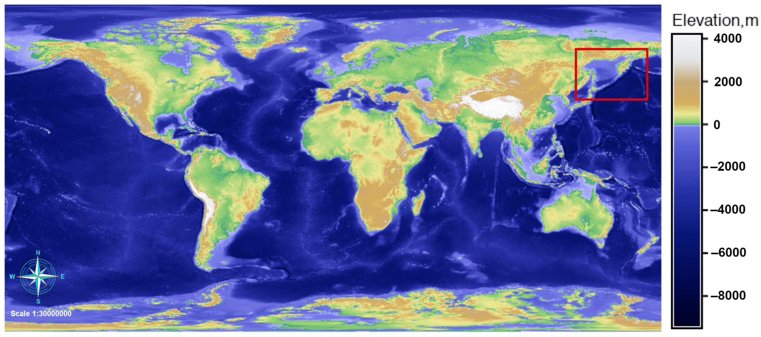
The heterogeneity in the topographic structure of the Kuril–Kamchatka region reflects the cumulative effects from the complex geological setting and tectonic processes in the north-west Pacific Ocean, which requires advanced cartographic methods for geospatial data processing. To this end, this study presents the application of the GRASS GIS, an open source powerful software for topographical modelling, visualization, statistical analysis, and mapping with a case study of morphometric data analysis. Besides open source availability, GRASS GIS includes a variety of functional tools for processing both raster and vector data, using both a graphical user interface (GUI) and scripts for mapping. Leaving the GUI approach as a more trivial approach of geospatial data processing, this paper presents the implementation of the scripting methods using the GRASS GIS. We present a case of topographical modelling and data handling integrating GRASS GIS with such libraries as the Geospatial Data Abstraction Library (GDAL) and PROJ as key tools for transforming geospatial data formats and cartographic projections. The combination of these technical tools introduces major computational challenges for cartographic data processing and selection of the best projection to avoid distortions [49].

The objective of this study is to provide effective geoprocessing using architecture of the GRASS GIS, enabling data storage in one location of the ‘mapset’. The ‘mapset’ in the GRASS GIS can be used for the same coordinate reference system and projection by interactive map design. The GRASS GIS modules were used to assess the morphometrics in the land-surface parameters over the study area based on the ETOPO1-derived basin morphometry: profile and tangential curvature, slope and aspect maps, and histograms of elevation distribution. As a result of the GRASS GIS application, the study revealed the effective coupling of scripting techniques and open source geospatial datasets in an optimised manner for modelling morphometric parameters and topographic mapping in a tectonically active region of the Pacific Ocean.

Current methods for geospatial data processing all focus on projecting the data according to the geospatial location. Thus, to enable data modelling, the QGIS and ArcGIS have a special modelling tool that allows one to create new tools with the use of sequential algorithms; while this can be a flexible solution for thematic maps, for topographical modelling this approach is unfeasible as placing different projections into separate folder locations is more optimal when dealing with several projections because it makes it possible to discriminate between the grids and process maps in distinct map sets. In contrast to traditional GIS software, the architecture of the GRASS GIS presents a collection of modules that can be stored as a sequence in a shell script and used for mapping using a console.

We instead focus on using the advantages of the GRASS GIS to demonstrate the effectiveness of scripts and data processing for mapping and visualization, as well as its compatibility with libraries GDAL, PROJ, and R [50,51,52,53]. The theoretical approaches in the morphometric studies [54] have been implemented in practical applications of GRASS GIS and developed in the GRASS GIS module r.slope.aspect [55], as demonstrated in this study. The topographical modelling and spatial analysis based on the continuous field of DEM assist in the analysis of slope stability in geologic risk assessment and its diverse applications in Earth sciences [56,57,58]. Selected features in the GRASS GIS function are comparable to the principles of other GIS. For instance, similar to QGIS, the technical flexibility of the GRASS GIS enables switching between the GUI and command-line mode of data processing. Similar to GMT, GRASS GIS uses a programming approach which enables the speeding up of repeated tasks through executable scripts.

Resembling the scripts in Unix shell, R and Python environments [59], GRASS GIS and GMT scripts are used to automate the workflow repeatedly performed for different maps using the same algorithm for various study areas. Other examples of automation of the cartographic workflow are diverse and include cases of rapid vectorisation of the isolines via machine learning [60], morphometric landscape analysis [61,62], geospatial analysis-based scripting libraries [63], topographic mapping using the GMT and QGIS [64], and fractal modelling quantifying the repetitive patterns [65].

Results from this study can be incorporated into a cartographic framework for spatial analysis of the morphometric structures in the west Pacific Ocean. The ability of GRASS GIS to smoothly handle large geospatial datasets, and improve and facilitate a cartographic workflow in various projects through automation is demonstrated in scripts. We present topographic mapping and morphometric surface modelling using several scripts of GRASS GIS. These results provide new perspectives for both cartographic workflow and topography-based spatial analysis in various fields such as applied geology. This paper also highlights the capabilities of mapping and modelling the bathymetric data by GRASS GIS for inaccessible deep marine and shelf areas. In contrast to terrain areas where fieldwork is possible, the submarine relief can only be evaluated and mapped by processing geospatial datasets using advanced cartographic methods.

2. Case Study

This study is focused on the Kuril–Kamchatka Trench and Kuril island arc that extend in the north-west Pacific Ocean, from the Kamchatka Peninsula to Hokkaido Island of the Japanese Archipelago, (Figure 1). This region is characterised by complex geological settings and high seismicity caused by the deep slab dynamics and morphology with high discontinuity of the subduction zone, as recently revealed in seismic cross-sections [66]. Thus, almost all of the islands from the Greater Kuril Chain are located along the submarine ridge of the Kuril island arc with depths of 100–300 m above them. Further, the morphological structure includes the submerged Vityaz ridge which extends from the ocean side of the Sea of Okhotsk. The Kuril–Kamchatka Trench generally has a flat seabed consisting of a chain of relatively wide and narrow segments representing short sections with depths of over −7000 m. However, it differs in the southern and northern parts with a maximum depth (−9717 m) recorded in its southwestern segment.

The basement surface of the Mesozoic structures near the northern coast of the Sea of Okhotsk forms a sub-latitudinal depression with depths reaching up to 3 km. Local minor trenches with depths of up to −2000 m extend from this depression in a sub-meridional direction, covering structural uplift in the centre of this sea. The southern part of the Sea of Okhotsk has a notable depression with depths exceeding −5000 m. The steep basement structures of the nearby shelf and the Kuril island arc descend towards the bottom of this depression.

The surface morphology of the seafloor basement in the Kuril–Kamchatka Trench correlates well with its modern relief. However, the depths of the seabed trenches are about −1000 to −2000 m deeper. According to the age of the constituent rocks, the Kuril–Kamchatka island arc was formed during the Oligocene period with some of the most ancient seamounts, mostly located on the slopes of the trenches, formed on the Mesozoic crust. Following the subduction of the tectonic plates under the island arcs, these seamounts were displaced from the basement surface and imprinted in the structures of the island arcs and coastal structures of the active continental margins. Such volcanic mountains are found, for instance, in the modern structures of the submarine slopes of the Kamchatka Peninsula.

The geophysical settings in the study area have a zone of linear positive and negative magnetic anomalies with an isometric magnetic field in the Kuril basin, which extends along the Kuril island arc and continues further within the Kamchatka Peninsula. The upper edges of the anomaly-forming bodies, associated with the volcanic rocks of the Pliocene-Quaternary age, are deposited closer to the surface. The geological complexity of the region of the Kuril–Kamchatka Trench and Kuril island arc, as briefly described above, illustrates the existing connectivity and correlation between the submarine and terrestrial morphology of the study area.

3. Materials and Methods

The research was implemented in the GRASS GIS [67], an open source software and image and graphics production system [68,69]. The major advantage of the GRASS GIS, similar to the QGIS, is that it combines the GUI with command-line interface (CLI) run from the console and enables operation with cartographic projections by GDAL. This makes it convenient to switch between the two modes of the data processing since it allows both cartographic and analytical experimentation with or without a traditional GUI menu. All the maps made in the GRASS GIS were stored using the Universal Transverse Mercator (UTM) map coordinate system, Zone 57, within the geographic extent of the study area. The full scripts used in this study for topographic mapping by the GRASS GIS are available in the GitHub repository of the authors with a provided open access using the following link: https://github.com/paulinelemenkova/Mapping_KKT_GRASS_GIS_Scripts (accessed on 18 February 2022).

The GRASS GIS uses a modular system organised by the name according to their functionality class (raster or vector) with the first letter indicating a function class, separated by dots and describing the specific task performed by this module. This feature is specific for GRASS GIS, yet differs from the GMT, a scripting cartographic toolset [70]. The console-based approach has distinct scripting toolsets from the GIS which mostly use the GUI as a main workflow environment. In contrast, the GRASS GIS enables the use of both GUI with a standard menu and a scripting approach, one of its advantages demonstrating its flexibility between the fully console-based GMT and the conventional GIS. This enables cartographic work to be performed in both ways, depending on the needs, preferences and profits from the combination of both approaches.

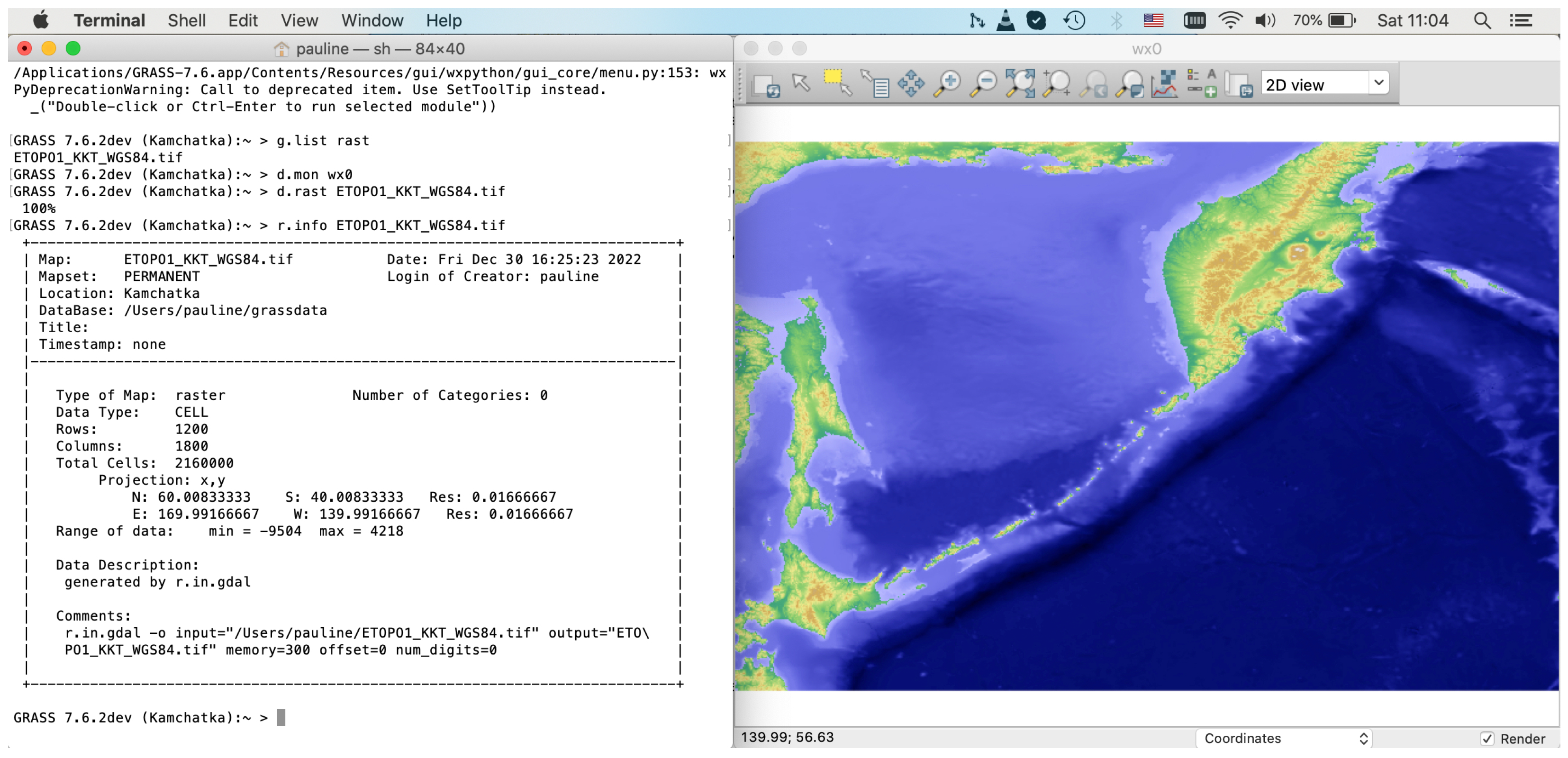
3.1. Data Capture and Organisation

The data used in this project include the open source datasets available online. The georeferenced Tag Image File Format (TIFF) file of the ETOPO1 grid by NOAA (https://www.ngdc.noaa.gov/mgg/global/ (accessed on 18 February 2022)) was used as a base map from the ETOPO1 Bedrock: Grid of Earth’s surface depicting the bedrock underneath the ice sheets, (Figure 1). The ‘gdalinfo’ module of the GDAL library was used to display raster metadata and the ‘gdalwarp’ was applied to project the initial raster file in the XY Cartesian coordinate into the WGS84. Likewise, the GDAL library ‘gdal_translate’ utility was used to subset target regions from the global grid; the GRASS GIS command-line modules r.info, d.mon, and d.rast were used for visualising the output raster. Metadata checking for raster maps was performed by the ‘g.list rast’ GRASS GIS module, (Figure 2). The information on the data grid was checked by the command ‘r.info’ module which returns the min/max coordinates of the study area, resolution, number of classes, cartographic projection, scale, geometry with the number of centroids, points, lines, boundaries and islands, and the type of data (3D or 2D).

The command ‘d.mon’ displays a raster map in a selected monitor. The monitors are used in the GRASS GIS system for visualization of various grids by the commands ‘d.mon wx0’ and ‘d.mon wx1’. The project management in GRASS GIS has a certain similarity to the ArcGIS in terms of data storage. Thus, each raster or vector map consists of several auxiliary files which include various data types, categories, header, and other specific information. The information on the projection of the current mapset was checked up by the commands: ‘g.proj-p’ (general description), ‘g.proj-w’ (here: the area of interest (AOI) extension and mathematical approximation are as follows: standard parallels, latitude of origin, central meridian, and false easting and northing). A summary of the algorithm used for plotting is presented in Listing 1:

Listing 1. GRASS GIS script for mapping ETOPO1 raster file.

1  #!/bin/sh

2  # raster file imported to the Location folder ‘Kamchatka’

3  r.in.gdal -o input = /Users/pauline/ETOPO1_KKT_WGS84.tif output = ETOPO1_KKT_WGS84.tif

4  # checked up the list of the raster files in the working directory

5  g.list rast

6  #starting graphical display (or ‘monitor’) in which the maps were displayed

7  d.mon wx0

8  # visualizing raster by d.rast utility which displays grid cell maps in the current graphics region

9  d.rast ETOPO1_Bed_g_geotiff

10  # changing color palette, from default viridis to srtm_plus

11  r.colors ETOPO1_KKT_WGS84 col = srtm_plus

12  # check of the range of the elevation values (depths/heights) of the map

13  r.info ETOPO1_KKT_WGS84

14  # display a legend on a map

15  d.rast.leg map = ETOPO1_KKT_WGS84

16  # providing numerical output of category numbers or range of values in a raster

17  r.describe ETOPO1_KKT_WGS84

18  # print a list of category numbers and associated labels

19  r.cats

20  # check up and print the current region extent (in this case: NS: 20.000000; EW: 45.000000).

21  g.region -e

22  # Removing auxiliary files

23  g.remove type = raster name = ETOPO1_KKT_WGS84.tiff -f

The trial directories were removed from the Unix utility ‘rm’ from a console by commands in two steps: (1) cd /Users/<…>/grassdata (changing to the current folder); (2) rm -r testKKT (here: removing testing folder for the Kuril–Kamchatka Trench with all files). The ‘g.region-p’ command was used to retrieve the information on the data extension and selected region (West, East, South, or North (WESN); number of rows; columns and cells; as well as additional cartographic data: ellipsoid, datum, and zone).

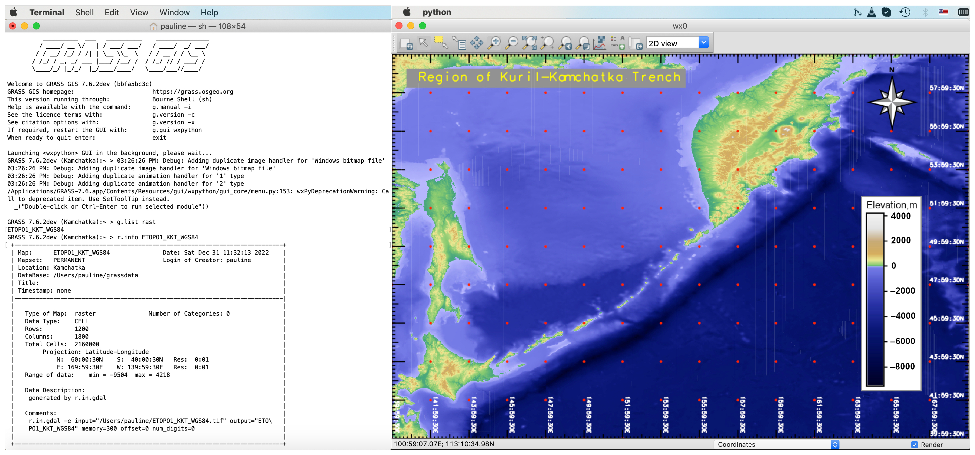
3.2. Data Processing by GDAL

The initial operations with raster files were performed by the Geospatial Data Abstraction Library (GDAL), a translator library for raster and vector geospatial data formats with available GDAL documentation [71]. The input to the reference list [71] was run from the GMT console. In general, the GDAL was used to re-project raster files to the supported cartographic projection, as well as to perform image mosaicking and transformations. In this study, we used three GDAL utilities using the commands of the following utilities:

‘$gdalwarp$’, ‘$gdal\_translate$’, and ‘$gdalinfo$’. The ‘gdalwarp’ utility was used for the re-projection and warping of the initial original file (ETOPO1_Bed_g_geotiff.tif) from the XY Cartesian coordinates to the World Geodetic System 1984 (WGS84) [72].

The PROJ library, used for transforming the projections, was installed via the Homebrew package manager using the following commands: ‘brew install proj’ and ’brew upgrade proj’ for installing and updating the package, respectively. The transformation uses the European Petroleum Survey Group (EPSG) number, which in this case is 4326 (corresponds to the WGS84). The warping was performed by the command for spatial reference system (SRS) as follows:

gdalwarp -tsrs EPSG:4326 ETOPO1Bedggeotiff.tif ETOPO1WGS84.tif

The next step entails running the utility ‘gdal_translate’ with the argument ‘-$projwin\_srs<srs\_def>$’, which specifies the projwin SRS GDAL, in which it interprets the coordinates (here, given coordinates in the EPSG system).

Using the gdal_translate, the file was subset, or clipped, to the target square area from the global extent with clockwise coordinates in degrees as follows: W = 140 N = 60 E = 170 S = 40. The re-projection was performed by the ‘gdalwarp’ utility and is illustrated in Figure 3. The subsetting of the target area was performed by the following command: gdaltranslate -projwin 140.0000 60.0000 170.0000 40.0000 ETOPO1WGS84.tif ETOPO1KKTWGS84.tif

Now that all the components of the code have been explained, we provide a summary in Listing 2.

Listing 2. GRASS GIS script for adding cartographic elements.

1  #!/bin/sh

2  g.region rast = ETOPO1_KKT_WGS84.tif -p

3  d.mon wx0

4  d.rast ETOPO1_KKT_WGS84

5  r.colors ETOPO1_KKT_WGS84 col = srtm_plus

6  d.legend raster = ETOPO1_KKT_WGS84 title = Elevation, m title_fontsize = 12

7  font = Helvetica fontsize = 8 -t -b bgcolor = white label_step = 2000 border_color = gray -f thin = 10

8  d.northarrow style = fancy_compass rotation = 0 label = N -w color = black fill_color = gray fontsize = 10

9  d.grid size = 02:00:00 -a -d color = red width = 0.1 fontsize = 8 text_color = white

10  d.text text = "Region of Kuril–Kamchatka Trench" color = yellow bgcolor = gray size = 8

The method presentation is shown by the projection transformation by GDAL utility ‘gralwarp’ using the PROJ library. It demonstrates the transformation of the TIFF file in the WGS84 geoid datum warped to a two-point equidistant azimuthal projection using the PROJ arguments:

gdalwarp -tsrs ’+proj=tpeqd +lat1=45 +lat2=55 +lon1=100 +lon2=120’ ETOPO1KKTWGS84.tif ETOPO1KKT2p.tif -overwrite

Now the file was reprojected to the WGS84 and subset (cut-off) from the initial raster grid with global extent. A gdalinfo utility was used to check the correctness of the performed operations and the output data as follows: $gdalinfoETOPO1\_KKT\_WGS84.tif.$ The standard parallels for the study area are 45${}^{\circ }$ N and 55${}^{\circ }$ N. Next, we present the code in Listing 3:

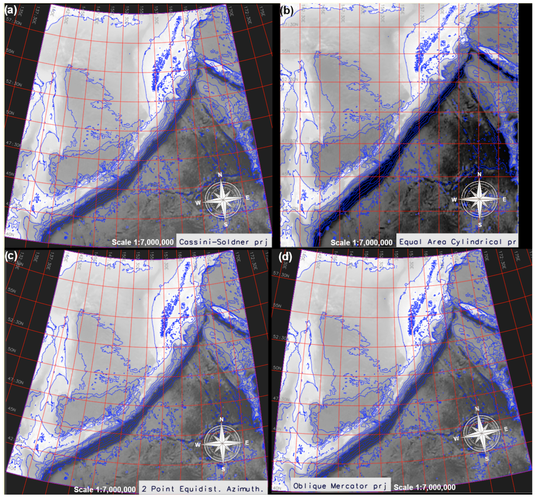
Listing 3. GRASS GIS script for plotting two-point equidistant azimuthal projection.

1  # stored in GeoTIFF in WGS84 warped to a Two-Point Equidistant Azimuthal projection:

2  gdalwarp -t_srs ’+proj = tpeqd +lat_1 = 45 +lat_2 = 55 +lon_1 = 100 +lon_2 = 120’ ETOPO1_KKT_WGS84.tif ETOPO1_KKT_2p.tif -overwrite

3  #!/bin/sh

4  g.list rast

5  r.info ETOPO1_KKT_2p

6  d.mon wx0

7  g.region raster = ETOPO1_KKT_2p -p

8  r.colors ETOPO1_KKT_2p col = grey.eq

9  d.rast ETOPO1_KKT_2p

10  d.redraw

11  r.contour ETOPO1_KKT_2p out = Bathymetry1000 step = 1000

12  d.vect Bathymetry1000 color = ‘blue’ width = 0

13  d.grid -g size = 2.5 color = ‘255:0:0’

14  d.text text = "2 Point Equidist. Azimuth." color = ‘0:0:51’ bgcolor = ‘224:224:224’ size = 3

The next step was continued in the GRASS GIS version 7.6 and included coordinate transformation, performed by ‘proj’ with several tested projections and their visualization using GRASS GIS scripts presented in Listing 4 for the Cassini–Soldner projection, Listing 5 for the oblique Mercator projection, and Listing 6 for the equal-area cylindrical projection. The ‘proj’ is a cartographic projection filter of the PROJ software which allows for converting between the geographic and projection coordinates within one datum WGS84. The maps projections were tested in PROJ via the ‘gdalwarp’ utility of GDAL before importing them into the GRASS GIS. The ‘gdalwarp’ is specifically designed to reproject maps to the target projections, coordinate systems, ellipsoid, or geodetic datum. In this case, we selected the datum as a constant WGS84 and kept it constant for this project.

The ellipsoidal Cassini–Soldner projection is well suited for the topographic mapping of areas with restricted extent along the meridian since the distortion of the areas along the central meridian is minimised (in this case, the meridian is 155${}^{\circ }$ E and latitude 50${}^{\circ }$ N). Thus, due to the more accurate computations in the ellipsoidal formulae, it provides a compromise between the conformal and equal-area projections keeping the distortions minimal in the longitudinal direction. The definition of this projection is based on the meridian and parallel of the central point of the study area. The plotting has been performed using the script provided in Listing 4.

Listing 4. GRASS GIS script for plotting map in Cassini–Soldner projection.

1  # stored in GeoTIFF in WGS84 warped to an Cassini (Cassini–Soldner) equirectangular projection:

2  gdalwarp -t_srs ’+proj = cass lat_0 = 50 lon_0 = 155’ ETOPO1_KKT_WGS84.tif ETOPO1_KKT_C.tif

3  #!/bin/sh

4  g.list rast

5  r.info ETOPO1_KKT_C

6  d.mon wx0

7  g.region raster = ETOPO1_KKT_C -p

8  r.colors ETOPO1_KKT_C col = grey.eq

9  d.rast ETOPO1_KKT_C

10  d.redraw

11  r.contour ETOPO1_KKT_C out = Bathymetry1000C step = 1000

12  d.vect Bathymetry1000C color = ‘blue’ width = 0

13  d.grid -g size = 2.5 color = ‘255:0:0’

14  d.text text = "Cassini–Soldner prj" color = ‘0:0:51’ bgcolor = ‘224:224:224’ size = 3

The geodetic transformations used to plot the map in the conformal oblique Mercator projection are expressed as a series of operations which represent the parallels and meridians as complex curves. These include the definition of the key parameters such as longitude and latitude of the projection centre, azimuth of the oblique equator with a scale along it representing the oblique aspect of the Mercator projection. The advantages of the oblique Mercator projection is that it provides a high accuracy in zones close to the longitude and latitude of the projection centre and a constant scale on the line of tangency, that is, the central longitude and preserves local shapes in regions of large lateral extent such as the Kuril–Kamchatka and Kuril islands. The map in the oblique Mercator projection was plotted using Listing 5.

Listing 5. GRASS GIS script for plotting map in oblique Mercator projection.

1  # stored in GeoTIFF in WGS84 warped to a Oblique Mercator projection:

2  gdalwarp -t_srs ’+proj = omerc +lat_1 = 45 +lat_2 = 55 lon_1 = 177 lon_2 = 210 +ellps = GRS80’ ETOPO1_KKT_WGS84.tif ETOPO1_KKT_OM.tif -overwrite

3  #!/bin/sh

4  g.list rast

5  r.info ETOPO1_KKT_OM

6  d.mon wx0

7  g.region raster = ETOPO1_KKT_OM -p

8  r.colors ETOPO1_KKT_OM col = grey.eq

9  d.rast ETOPO1_KKT_OM

10  r.contour ETOPO1_KKT_OM out = Bathymetry1000OM step = 1000

11  d.vect Bathymetry1000OM color = ‘blue’ width = 0

12  d.grid -g size = 2.5 color = ‘255:0:0’

13  d.text text = "Oblique Mercator prj" color = ‘0:0:51’ bgcolor = ‘224:224:224’ size = 3

The key parameters for defining the equal-area cylindrical projection include the latitude (the meridian) of the true scale or standard parallels (in this case, 50${}^{\circ }$ N and 155${}^{\circ }$ E). The distortions along the central meridian and parallels are minimised since they provide a centre point of the extent of the study area. The projection has been defined by the ’gdalwarp’ and then plotted using the scripting in Listing 6:

Listing 6. GRASS GIS script for plotting map in Equal-Area Cylindrical projection.

1  # stored in GeoTIFF in WGS84 warped to an Equal Area Cylindrical projection:

2  gdalwarp -t_srs ’+proj = cea lat_ts = 50 lon_0 = 155’ ETOPO1_KKT_WGS84.tif ETOPO1_KKT_EAC.tif

3  #!/bin/sh

4  g.list rast

5  r.info ETOPO1_KKT_EAC

6  d.mon wx0

7  g.region raster = ETOPO1_KKT_EAC -p

8  r.colors ETOPO1_KKT_EAC col = grey.eq

9  d.rast ETOPO1_KKT_EAC

10  d.redraw

11  r.contour ETOPO1_KKT_EAC out = Bathymetry1000 step = 1000

12  d.vect Bathymetry1000 color = ‘blue’ width = 0

13  d.grid -g size = 2.5 color = ‘255:0:0’

14  d.text text = "Equal Area Cylindrical prj" color = ‘0:0:51’ bgcolor = ‘224:224:224’ size = 3

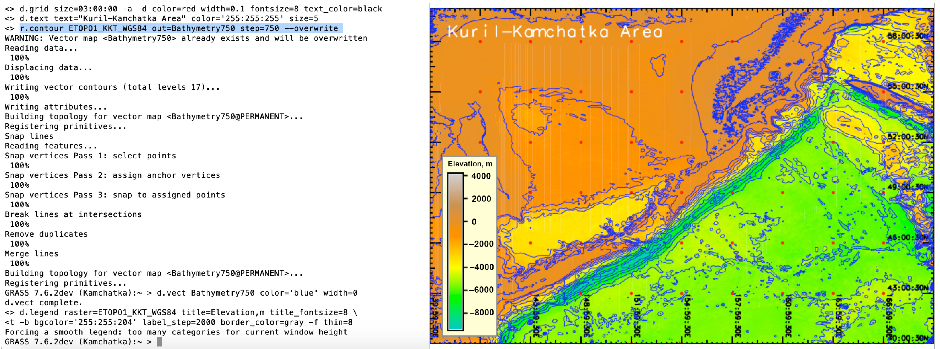
3.3. Displaying Raster Grids in GRASS GIS

Upon re-projection of the file, it was imported to the GRASS GIS by the ‘r.in.gdal’ utility. Displaying the dataset was performed using the sequence of the GRASS modules shown in Listing 1, based on the GRASS GIS modular techniques [73] and visualized in Figure 2. The visualized cartographic elements include grid ticks, legend and the title, which were placed on the map in Figure 3 using the code in Listing 2. Generating the continuous fields of the bathymetric contours (isolines) were derived from the raster ETOPO1_KKT_WGS84 file using the GRASS GIS module ‘r.contour’ by script. In this example the step parameter was set to 750 m and is visualized in Figure 4. The script of the GRASS GIS used for plotting the topographic isolines is shown in Listing 7:

Listing 7. GRASS GIS script for visualising raster grid and adding contour isolines.

1  #!/bin/sh

2  d.mon wx0

3  r.info ETOPO1_KKT_WGS84

4  g.region raster = ETOPO1_KKT_WGS84 -p

5  d.rast ETOPO1_KKT_WGS84

6  d.grid size = 03:00:00 -a -d color = red width = 0.1 fontsize = 8 text_color = white

7  d.text text = "Kuril–Kamchatka Area" color = ‘255:255:255’ size = 5

8  r.contour ETOPO1_KKT_WGS84 out = Bathymetry750 step = 750 –overwrite

9  d.vect Bathymetry750 color = ‘102:37:4’ width = 0

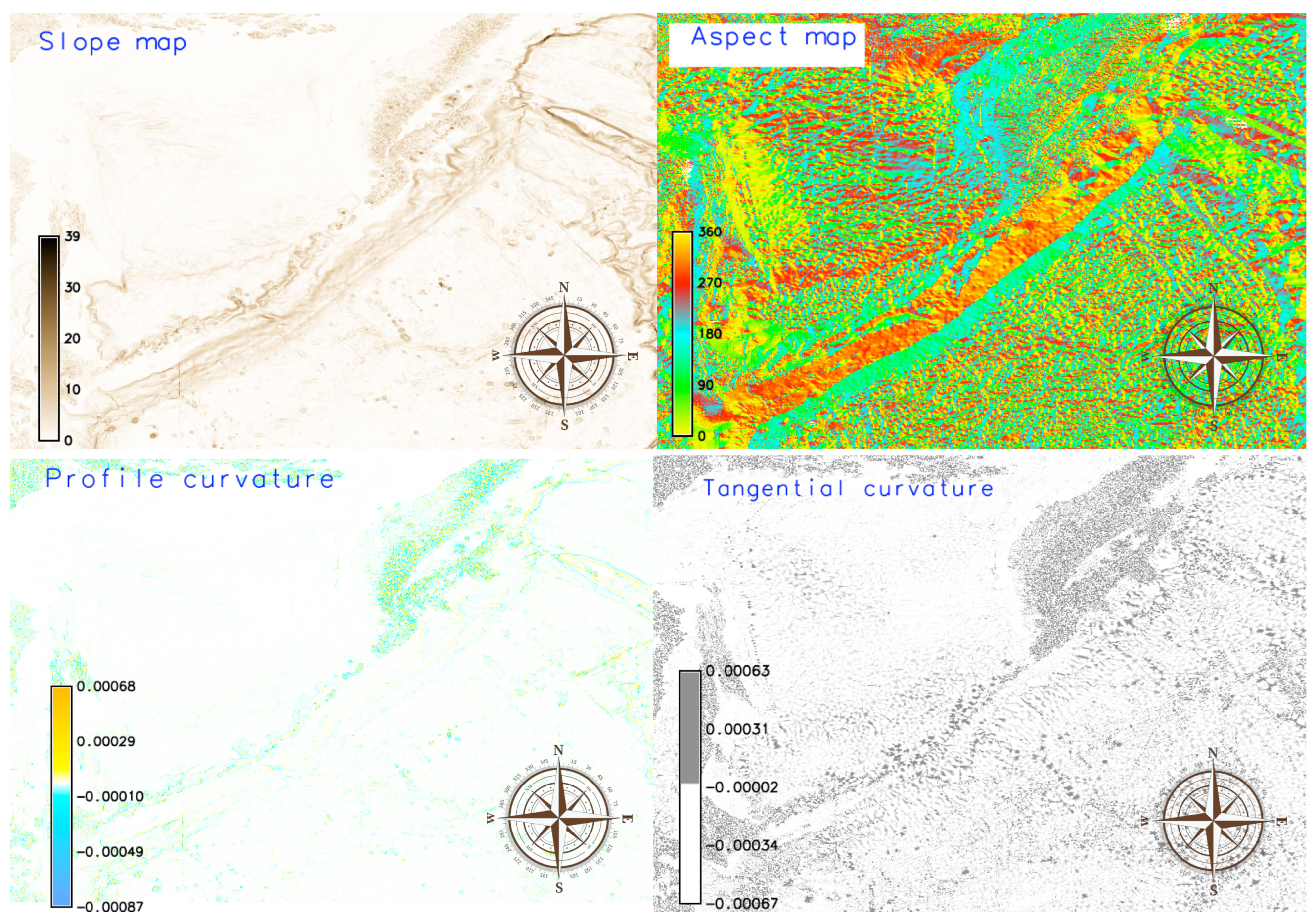
3.4. Calculating Morphometric Parameters

The correlation between the profile and tangential curvature reflects the methodological approaches of the algorithm which concerns the mathematical approximation of the morphological profile of the slopes and inflation of the terrain heights. The differences in calculus are well-illustrated in Equation (1) for the profile curvature $K_P$[74] and Equation (2) for the tangential curvature $K_T$ [74].

$$K_P=\frac{\left(\frac{{\delta }^{2}z}{\delta x^2}\right){\left(\frac{\delta z}{\delta x}\right)}^2+2\left(\frac{{\delta }^{2}z}{\delta x\delta y}\frac{\delta z}{\delta x}\frac{\delta z}{\delta y}\right)+\frac{{\delta }^{2}z}{\delta y^2}{\left(\frac{\delta z}{\delta x}\right)}^2}{p{q}^{\frac{3}{2}}}$$

(1)

$$K_T=\frac{\left(\frac{{\delta }^{2}z}{\delta x^2}\right){\left(\frac{\delta z}{\delta y}\right)}^2-2\left(\frac{{\delta }^{2}z}{\delta x\delta y}\frac{\delta z}{\delta x}\frac{\delta z}{\delta y}\right)+\frac{{\delta }^{2}z}{\delta y^2}{\left(\frac{\delta z}{\delta x}\right)}^2}{p{q}^{\frac{1}{2}}}$$

(2)

where $p={\left(\frac{\delta z}{\delta x}\right)}^2+{\left(\frac{\delta z}{\delta y}\right)}^2$ and $q=1+p$ for both cases.

The plotting of the morphometric parameters was performed using the code:

‘r.slope.aspect elevation=ETOPO1KKTWGS84 slope=slope aspect=aspect pcurvature=pcurv tcurvature=tcurv’

where the input elevation raster map is the ETOPO1_KKT_WGS84, and the output raster map is ‘slope’. The curvature shows the rate of variations of the slope, which makes it the second function of the elevation variable related to the surface heights [75]. This process technically includes both cases: whether the purpose is profile or tangential curvature. However, the difference is in the approaches of the mathematical algorithms that are embedded in the GRASS GIS. Hence, the difference between the profile and tangential curvature consists of the method of calculation. For the tangential curvature, it is computed as perpendicular to the slope gradient, while for profile curvature, it measures a curvature of the surface in the direction of the gradient [76]. The slope shows a steepness or the degree in the topographic surface covering the study area. The aspect, or exposure, is a compass direction that a slope faces (East, West, South, or North). Geographically, the aspect of a slope has a significant impact on the local microclimate which affects physical and often botanical features of a mountain slope, i.e., a slope effect on the terrestrial areas.

Such effects are owing to the strong correlation between the mountain slope and temperature, which is in turn affected by the angle of sun. Hence, both parameters are derivative from the slope of the elevation with certain variations in the mathematical approach and angle direction of the gradient degree (direct and perpendicular). The theoretical foundations of the slope and angle modelling in geospatial research can be found in existing works reporting, for instance, on the effects from the cell size [77], gradient angles [78], numerical terrain analysis [79], or quantifying land surface and slope curvatures [80,81,82,83]. The increase in values of a specific depth was analysed by plotting the histograms as bars and pie charts using the GRASS GIS ’d.histogram’ module for calculating depths distribution [84]. The visualized images are displayed using various colour map palettes (r.colors) specifically intended for the cartographic visualization of the terrain raster grids.

4. Results and Discussion

The GRASS GIS algorithms were implementedfor cartographic data visualization and map compilation in various projections. The topographic data visualization and a morphometric analysis were based on the GRASS GIS modules. The input cartographic data based on the ETOPO1 raster grid comprised the derived variables: slope, aspect, curvature, and hillshade. The data analysis included a plotted histogram and pie chart showing data distribution. Several projections were tested and visualized using the PROJ library. The data transformation was performed using GDAL integrated with the GRASS GIS.

4.1. Cartographic Projections by PROJ

The PROJ, a generic coordinate transformation software library [85], was used to transform the raster grid files in Lat/Lon geospatial coordinates from one coordinate reference system (CRS) to another. This method includes the PROJ transformation which performs a variety of operations with cartographic data, starting from the simple and well-known projections such as cylindrical Mercator projection to the very complex transformations across many reference coordinate frames. The PROJ was used for testing various projections (conic, cylindrical, and azimuthal) selected from a variety of available projections in the library: Cassini–Soldner equirectangular; equal area cylindrical; two-point equidistant azimuthal; and oblique Mercator [86].

Originally made as a technical tool for cartographic projections, PROJ gradually transformed into being a functional generic coordinate transformation engine. The supported projections were checked by the command ‘cs2cs -lp’ from the GRASS GIS console [87]. The PROJ was applied for the scale cartographic projections and coordinate transformation (Figure 5), thus presenting the geodetic transformations of varying complexity. In this study, the visualization of various cartographic projections in GRASS GIS (Figure 5) was performed by a combination and sequential use of the following modules of GRASS GIS: ‘d.rast’, ‘r.contour’, ‘d.vect’, ‘d.grid’, and ’d.text’. The script is based on the developed methodology of data processing by GRASS GIS [88]. It was used for plotting the contour maps with an example of Cassini–Soldner projection. Mapping the study area in various cartographic projections was recorded in separate plots in the GRASS GIS and is presented in Figure 5 for comparison: Cassini–Soldner equirectangular; equal area cylindrical; two-point equidistant azimuthal; and oblique Mercator.

4.2. Morphometric Parameters

The input elevation data were derived from the ETOPO1 raster grid containing the elevation values in a digital format covering the study area. The ‘r.slope.aspect’ module of GRASS GIS was used to plot raster maps using the developed methodology [55,89,90]. The resulting maps of slope, aspect (computed counterclockwise from the east), profile curvature, and tangential curvature from the ETOPO1 raster grid are shown in Figure 6. The results include the morphometric elements of slope, aspect, profile curvature, and tangential curvature (Figure 6).

The results of the morphometric modelling show that the terrain slope in the Kuril–Kamchatka region ranges from 0${}^{\circ }$ to 39${}^{\circ }$, as shown on the slope map calculated from the ETOPO1_KKT_WGS84 grid. The slope in the study area is shown in gradually increasing degrees starting from 0${}^{\circ }$ (flat horizontal) to 39${}^{\circ }$ (maximal vertical). The profile curvature shows modelled terrain surfaces in the gradient direction which reflects the variations in the slope steepness angle within the range of −87 × 10${}^{-5}$ to 68 × 10${}^{-5}$. The largest area coloured light green on the lower left map (Figure 6) has values of −10 × 10${}^{-5}$ to 0. Practically, it indicates that the velocity of mass falls downwards along the slope curve. The tangential curvature reflects the change in the aspect angle and influences the divergence, or convergence, of the water flow, respectively.

The tangential curvature shows values of −67 × 10${}^{-5}$ to 63 × 10${}^{-5}$. The terrestrial areas of the Kamchatka Peninsula and Greater Kuril Chain show higher positive values, depicted by the dark grey colours, in the lower right map (Figure 6) compared to the water areas of the Sea of Okhotsk (white and light grey colours) which shows variations in the land surface steepness over the terrain compared to water areas. Numerically, the aspect map shows the orientation in degrees varying from 0${}^{\circ }$ to 360${}^{\circ }$ (upper right map in Figure 6). It shows a clear correlation between the aspect and topographic area of the Kuril–Kamchatka Trench (130${}^{\circ }$–150${}^{\circ }$, emerald green colour on the map) and the Greater Kuril Chain which extends in parallel to the trench both in the southeastern orientation (beige colour from the selected ‘aspectcolr’ colour palette, 300${}^{\circ }$–330${}^{\circ }$, ). A clear delineation of the Sakhalin Island can be noted as the north-western orientation (yellow-green colours, 0${}^{\circ }$–30${}^{\circ }$, ) and the Kamchatka Peninsula (NW, greens, 60${}^{\circ }$–120${}^{\circ }$).

The produced maps show morphometric variables over the target area performed by the GRASS GIS techniques which include data conversion, warping, transforming projections, and adding cartographic elements (ticks, legend, and isolines) on the final layout. Each map sources a range of new visualizations of the data relevant to the morphology of the study region. Similar to the GMT techniques, the scripting methods of the GRASS GIS have a command-line approach of data processing. This is convenient for controlling the cartographic design and enables the creation of print-quality maps. Further, we demonstrated the effectiveness of the GRASS GIS methods in visualising raster grids and performing raster data analysis in a geologically complex region, such as the northwestern sector of the Pacific Ocean. The computed geomorphic indices included slope, aspect, profile, and tangential curvature maps, derived from the topographic grid using the embedded algorithms in GRASS GIS.

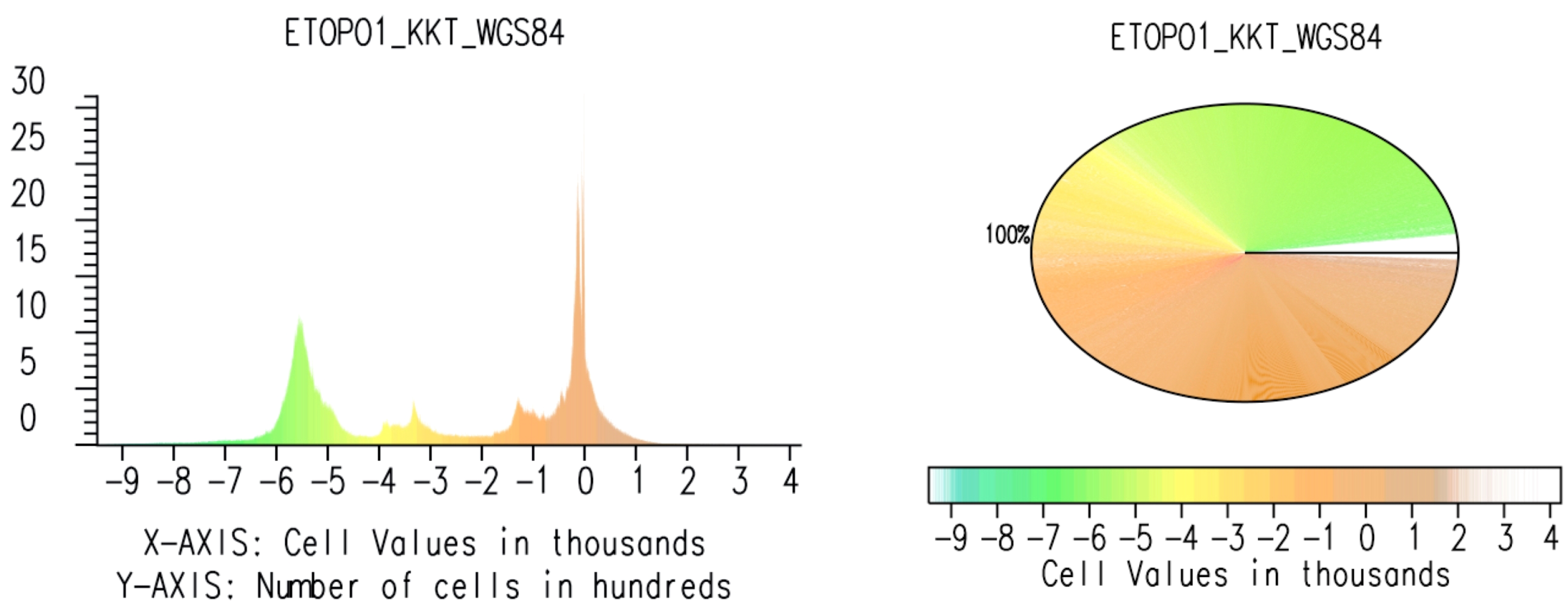
4.3. Analysis of the Elevation Frequency

The next research step included the analysis of the distribution of the elevation over the study area. Using computational techniques of GRASS GIS, we calculated the frequency of the data in various range diapason and the repeatability of corresponding depths. The most frequent depths or elevations over the study area were recorded and summarised for the analysis of spatially distributed data [91,92,93]. The increase in values of a specific depth reflects the frequency of the elevation recorded on a bathymetric and topographic grid in a subsequent region of the study area. The analysis of the spatial data distribution aimed to demonstrate a range of variations in data, including skewness, the variation of values within intervals of the topography, organisation of categorical data, selecting relevant peaks in the interpretation and description of the dataset, or other resources showing the correlation among the morphometric parameters, such as the aspect and slope with relief. The distribution of topographic data has been evaluated using statistical tools embedded in GRASS GIS and presented in a histogram and a pie chart (Figure 7).

The critical synthesis and analysis of a geomorphological setting of the study area is largely based on the experiential techniques of cartographic data visualization using GRASS GIS. A range of its modules utilised in scripts for cartographic transformations were used to visualise various projection and colour map palettes. The topographic data analysis demonstrated variations in the percentage of data distribution and morphometry in the study area, as follows. The depths in the interval below 400 to −2000 m covered 24% of the total points; the depths in the interval from −2000 to −3000 m summed to 2%; the depth from −3000 to −4000 m took up 4% of the total points; the depths in the range between −5000 and −6000 m were 13%; and the depth in the diapason from −6000 to 7000 m were less than 1%. The rest of the elevation points are covered by the data with the diverse heights and topographic values.

The extent of the data range is summarised and visualized in the histogram and pie chart (Figure 7). The bar plot and the pie chart show the frequencies of the elevation levels in a raster representing morphometric unevenness of the terrain. For each topographic range, the number of pixels in the raster image is counted and drawn on the diagram in the two views of representation. The number of pixels corresponding to the each value of depth/height contributes to the height of this particular bar on the chart (or a radius of a segment in the pie). The x-axis of the bar chart diagram represents the topographic/bathymetric values (heights and depths), while the vertical y-axis shows the number of pixels counted at a given step.

The morphometry is an essential approach of quantitative GIS-based terrain analysis. It is increasingly used in diverse geological applications for relief visualization. Based on elevation derived from DEM, the landforms can be visualised in the target area for morphological modelling and mapping at regional scale. The morphometric terrain analysis may further include extended approaches such as analysis and interpretation of the land forms or seafloor surface as a continuous field, and upscaling the morphological shapes for a closer analysis of the terrain structure. The slope gradient indicates the terrain roughness and represents a base for the land surface discreteness. A slope gradient can be used as an indication of terrain roughness, while the aspect can be applied for mapping slope distribution, depending on the compass orientation of the terrain.

The findings revealed that the topography of the Kuril–Kamchatka Trench varied significantly reflecting its regional geologic evolution and tectonic setting which largely affects the structure of the relief. Our study presented a case for displaying topographic data to analyse height differences using cartographic and statistical data processing. We have shown a specific example of bathymetric data processing for the north Pacific Ocean area performed using a scripting approach by GRASS GIS syntax with its specific language operated from the command line. The scripts of the GRASS GIS were used to rapidly plot the topographic data as a series of morphometric variables. The results can be extended to similar datasets using scripts presented for the repeatability of data processing in GRASS GIS: visualization of the slope, aspect, curvature, and statistical data distribution of elevation data.

5. Conclusions

Advancing insights into the complexities of the heterogeneous bathymetry and topography in coastal areas can be enhanced through the application of advanced cartographic tools. We applied the ETOPO1 World Global Relief Model data on the western segment of the Pacific Ocean to quantify morphometric terrain parameters and evaluate the performance of various cartographic projections by spatial data transformation in the GRASS GIS environment. ETOPO1 data provided detailed information on the variations in the topographic structure over the target region. We modelled slope, aspect, profile curvature and tangential curvature using a combination of the GRASS GIS modules presented in scripts coupled with the GDAL library for data transformation and formatting. The results of the topographic modelling were statistically processed for analysis of the depth and heights distributions over the study area to evaluate the heterogeneity of landform elements.

The integration of the GRASS GIS scripts with geospatial data allowed us to characterise the distribution of elevation values throughout the region. Using such an approach, this paper revealed the value of spatial data processing to model morphometric parameters by GRASS GIS scripts in semi-automatic topographic mapping. As a result, we found and visualised the high complexity of land surface structures and adjacent bathymetry in the region, linked to the geological and tectonic processes that shaped the current landforms. The variations in the slope and aspect maps were evaluated along with the profile and tangential curvature of the topographic dataset to model the curvature of the relief in the Kuril–Kamchatka region. Topographic mapping and morphometric modelling rely on spatial data processing and representation. However, real-world spatial data are generated from DEM involving may factors. These include the geologic drivers and tectonic processes in the past that affect modern relief of the Earth.

Such complexity of the relief is reflected in the diverse datasets with various resolution and details of the land surface. Processing these data and visualising the topography of the Earth with variability of the morphometric patterns requires the advanced tools of cartographic representation and automated approaches of data handling. As a result, recent efforts have been made to integrate the programming tools into the GRASS GIS for geospatial studies. To this end, we propose the use of the GRASS GIS modules for morphometric modelling and cartographic reprojecting the raster grids on selected area of the north-west Pacific Ocean. We demonstrate that the GRASS GIS is effective in terms of cartographic visualization and accuracy of spatial data processing. In addition, we provide a series of scripts used for plotting and data visualization as a reference in similar studies.

The application of the GRASS GIS algorithms aimed at topographic mapping and morphometric modelling that uses a script-based approach for cartographic data visualization, transformation, and analysis. The selected region of the tested area includes the northwestern segment in the Far East based on the ETOPO1 grid. The extensive experimental results on mapping of the raster images by scripts show that GRASS GIS outperforms the traditional software in terms of automating data processing which increases the speed and accuracy of cartographic plotting and, specifically, modelling the morphometric parameters. The latter include slope, aspect, and curvature in both the down-slope and across-slope directions, which is presented in this case study based on the GRASS GIS modules.

The results show the effective application of the GRASS GIS techniques for cartographic data processing. Using the console in scripting mode, we identified topographic variability in the target area through spatial analysis of the processed data and visualised raster grids in various cartographic projections. We have also shown that the geodetic transformation of the dataset in various cartographic projections performs well using the GDAL utility and PROJ library, while the choice of the cartographic projections is wholly due to the spatial location of the study area controlled by the possible distortions in sizes, angles, distances, and directions of the visualized objects. We demonstrated the method to be flexible in changing projections using the integration of GRASS GIS and GDAL.

With regard to addressing the cartographic plotting, GRASS GIS shows robustness and effectiveness of data handling both using the GUI and from the console in a series of listings. We believe that techniques of GRASS GIS for handling geospatial data can be further extended to deal with spatial datasets using scripts presented in this study. Thus, the advantage of this study is that it provides the scripts in the GitHub open repository that can be reused in similar studies for repeatability. These scripts are sequential used for algorithms from the GRASS GIS and composed with the use of several modules for topographic modelling and mapping.

References

1. Wang, J.; Wu, F. Advances in Cartography and Geographic Information Engineering; Springer: Singapore, 2022; Volume 638. [Google Scholar] [CrossRef]
2. Minár, J.; Evans, I.S.; Jenčo, M. A comprehensive system of definitions of land surface (topographic) curvatures, with implications for their application in geoscience modelling and prediction. Earth-Sci. Rev. 2020, 211, 103414. [Google Scholar] [CrossRef]
3. Maxwell, A.E.; Shobe, C.M. Land-surface parameters for spatial predictive mapping and modeling. Earth-Sci. Rev. 2022, 226, 103944. [Google Scholar] [CrossRef]
4. Zhou, W. GIS for Earth Sciences. In Encyclopedia of Geology, 2nd ed.; Alderton, D., Elias, S.A., Eds.; Academic Press: Oxford, UK, 2021; pp. 281–293. [Google Scholar] [CrossRef]
5. Ruzickova, K.; Ruzicka, J.; Bitta, J. A new GIS-compatible methodology for visibility analysis in digital surface models of earth sites. Geosci. Front. 2021, 12, 101109. [Google Scholar] [CrossRef]
6. Deseilligny, M.; Le Men, H.; Stamon, G. Map understanding for GIS data capture: Algorithms for road network graph reconstruction. In Proceedings of the 2nd International Conference on Document Analysis and Recognition (ICDAR ’93), Tsukuba, Japan, 20–22 October 1993; pp. 676–679. [Google Scholar] [CrossRef]
7. Sasso, D.; Biles, W.E. An object-oriented programming approach for a GIS data-driven simulation model of traffic on an inland waterway. In Proceedings of the 2008 Winter Simulation Conference, Miami, FL, USA, 7–10 December 2008; pp. 2590–2594. [Google Scholar] [CrossRef] [Green Version]
8. Rathod, N.; Subramanian, R.; Sundaresan, R. Data-Driven and GIS-Based Coverage Estimation in a Heterogeneous Propagation Environment. In Proceedings of the 2018 IEEE Global Communications Conference (GLOBECOM), Abu Dhabi, United Arab Emirates, 9–13 December 2018; pp. 1–6. [Google Scholar] [CrossRef]
9. Shrestha, B.; Devarakonda, R.; Palanisamy, G. An open source framework to add spatial extent and geospatial visibility to Big Data. In Proceedings of the 2014 IEEE International Conference on Big Data (Big Data), Washington, DC, USA, 27–30 October 2014; pp. 64–66. [Google Scholar] [CrossRef]
10. Scott, G.J.; Angelov, G.A.; Reinig, M.L.; Gaudiello, E.C.; England, M.R. cvTile: Multilevel parallel geospatial data processing with OpenCV and CUDA. In Proceedings of the 2015 IEEE International Geoscience and Remote Sensing Symposium (IGARSS), Milan, Italy, 26–31 July 2015; pp. 139–142. [Google Scholar] [CrossRef]
11. Scott, G.J.; Backus, K.; Anderson, D.T. A multilevel parallel and scalable single-host GPU cluster framework for large-scale geospatial data processing. In Proceedings of the 2014 IEEE Geoscience and Remote Sensing Symposium, Quebec City, QC, Canada, 13–18 July 2014; pp. 2475–2478. [Google Scholar] [CrossRef]
12. Chen, T.; Yuan, H.y.; Yang, R.; Chen, J. Integration of GIS and Computational Models for Emergency Management. In Proceedings of the 2008 International Conference on Intelligent Computation Technology and Automation (ICICTA), Changsha, China, 20–22 October 2008; Volume 2, pp. 255–258. [Google Scholar] [CrossRef]
13. Li, G.; Zhang, J.; Wang, N. Construction and Implementation of Spatial Analysis Model Based on Geographic Information System (GIS)—A Case Study of Simulation for Urban Thermal Field. In Proceedings of the 2008 International Conference on Computational Intelligence for Modelling Control & Automation, Vienna, Austria, 10–12 December 2008; pp. 1095–1098. [Google Scholar] [CrossRef]
14. Zhang, J.; Luo, W.; Yuan, L.; Mei, W. Shortest path algorithm in GIS network analysis based on Clifford algebra. In Proceedings of the 2010 2nd International Conference on Future Computer and Communication, Wuhan, China, 21–24 May 2010; Volume 1, pp. 432–436. [Google Scholar] [CrossRef]
15. Huang, Z.; Fang, Y. A novel approach for geospatial computational task processing in Grid environment. In Proceedings of the 2010 IEEE International Geoscience and Remote Sensing Symposium, Honolulu, HI, USA, 25–30 July 2010; pp. 3980–3982. [Google Scholar] [CrossRef]
16. Franges, S.; Zupan, R. New encouragement on cartographic visualisation. In Proceedings of the ISPA 2001—Proceedings of the 2nd International Symposium on Image and Signal Processing and Analysis—In conjunction with 23rd International Conference on Information Technology Interfaces (IEEE Cat.), Pula, Croatia, 19–21 June 2001; pp. 368–372. [Google Scholar] [CrossRef]
17. Zhang, B.; Ran, H.; Yu, J. Visualizaiton of water system based on the cartographic presentation. In Proceedings of the 2012 International Symposium on Geomatics for Integrated Water Resource Management, Lanzhou, China, 19–21 October 2012; pp. 1–4. [Google Scholar] [CrossRef]
18. Yamaguchi, N. Visualizing states in autoregressive hidden Markov models using generative topographic mapping. In Proceedings of the 2012 8th International Conference on Natural Computation, Chongqing, China, 29–31 May 2012; pp. 138–142. [Google Scholar] [CrossRef]
19. Pazouki, E. A smart surface irrigation design based on the topographical and geometrical shape characteristics of the land. Agric. Water Manag. 2023, 275, 108046. [Google Scholar] [CrossRef]
20. Moreira, E.P.; Valeriano, M.M. Application and evaluation of topographic correction methods to improve land cover mapping using object-based classification. Int. J. Appl. Earth Obs. Geoinf. 2014, 32, 208–217. [Google Scholar] [CrossRef]
21. Chowdhury, M.S. Modelling hydrological factors from DEM using GIS. MethodsX 2023, 10, 102062. [Google Scholar] [CrossRef] [PubMed]
22. Boulton, S.J.; Stokes, M. Which DEM is best for analyzing fluvial landscape development in mountainous terrains? Geomorphology 2018, 310, 168–187. [Google Scholar] [CrossRef]
23. Buterez, C.; Olariu, B.; Mihai, B.; Rujoiu-Mare, M.; Cruceru, I. General topography of Prahova County, Romania. J. Maps 2016, 12, 541–545. [Google Scholar] [CrossRef] [Green Version]
24. Duncan, D.T.; Regan, S.D. Mapping multi-day GPS data: A cartographic study in NYC. J. Maps 2016, 12, 668–670. [Google Scholar] [CrossRef] [Green Version]
25. Duarte, L.; Teodoro, A.C.; Sousa, J.J.; Pádua, L. QVigourMap: A GIS Open Source Application for the Creation of Canopy Vigour Maps. Agronomy 2021, 11, 952. [Google Scholar] [CrossRef]
26. Armstrong, M.P. Geography and computational science. Ann. Am. Assoc. Geogr. 2000, 90, 146–156. [Google Scholar] [CrossRef]
27. Duarte, L.; Teodoro, A.C.; Maia, D.; Barbosa, D. Radio Astronomy Demonstrator: Assessment of the Appropriate Sites through a GIS Open Source Application. ISPRS Int. J. Geo-Inf. 2016, 5, 209. [Google Scholar] [CrossRef] [Green Version]
28. Brovelli, M.A.; Mitasova, H.; Neteler, M.; Raghavan, V. Free and open source desktop and Web GIS solutions. Appl. Geomat. 2012, 4, 65–66. [Google Scholar] [CrossRef]
29. Christl, A. Free Software and Open Source Business Models. In Open Source Approaches in Spatial Data Handling; Advances in Geographic Information Science; Hall, G.B., Leahy, M.G., Eds.; Springer: Berlin, Germany, 2008; Chapter 2; pp. 21–48. [Google Scholar] [CrossRef]
30. Turton, I. Geo Tools. In Open Source Approaches in Spatial Data Handling; Springer: Berlin/Heidelberg, Germany, 2008; pp. 153–169. [Google Scholar] [CrossRef] [Green Version]
31. Barnes, N. Publish your computer code: It is good enough. Nature 2010, 467, 753. [Google Scholar] [CrossRef] [PubMed] [Green Version]
32. Issaka, Y.; Kumi-Boateng, B. Artificial intelligence techniques for predicting tidal effects based on geographic locations in Ghana. Geod. Cartogr. 2020, 46, 1–7. [Google Scholar] [CrossRef] [Green Version]
33. Lemenkova, P.; Debeir, O. Quantitative Morphometric 3D Terrain Analysis of Japan Using Scripts of GMT and R. Land 2023, 12, 261. [Google Scholar] [CrossRef]
34. Ajvazi, B.; Czimber, K. A comparative analysis of different DEM interpolation methods in GIS: Case study of Rahovec, Kosovo. Geod. Cartogr. 2019, 45, 43–48. [Google Scholar] [CrossRef] [Green Version]
35. Guan, Q.; Hu, S.; Liu, Y.; Yun, S. High-Performance GeoComputation with the Parallel Raster Processing Library. In GeoComputational Analysis and Modeling of Regional Systems; Springer International Publishing: Cham, Switzerland, 2018; pp. 55–74. [Google Scholar] [CrossRef]
36. Kralidis, A.T. Geospatial Open Source and Open Standards Convergences. In Open Source Approaches in Spatial Data Handling; Springer: Berlin/Heidelberg, Germany, 2008; pp. 1–20. [Google Scholar] [CrossRef]
37. Wagemann, J.; Siemen, S.; Seeger, B.; Bendix, J. Users of open Big Earth data—An analysis of the current state. Comput. Geosci. 2021, 157, 104916. [Google Scholar] [CrossRef]
38. Basith, A.; Prastyani, R. Evaluating ACOMP, FLAASH and QUAC on Worldview-3 for satellite derived bathymetry (SDB) in shallow water. Geod. Cartogr. 2020, 46, 151–158. [Google Scholar] [CrossRef]
39. Habib, M.; Alfugara, A.; Pradhan, B. A low-cost spatial tool for transforming feature positions of CAD-based topographic mapping. Geod. Cartogr. 2019, 45, 161–168. [Google Scholar] [CrossRef] [Green Version]
40. Yin, Z.; Li, J.; Liu, Y.; Xie, Y.; Zhang, F.; Wang, S.; Sun, X.; Zhang, B. Water clarity changes in Lake Taihu over 36 years based on Landsat TM and OLI observations. Int. J. Appl. Earth Obs. Geoinf. 2021, 102, 102457. [Google Scholar] [CrossRef]
41. Chen, L.; Ma, Y.; Lian, Y.; Zhang, H.; Yu, Y.; Lin, Y. Radiometric Normalization Using a Pseudo-Invariant Polygon Features-Based Algorithm with Contemporaneous Sentinel-2A and Landsat-8 OLI Imagery. Appl. Sci. 2023, 13, 2525. [Google Scholar] [CrossRef]
42. Rey, S.J. Code as Text: Open Source Lessons for Geospatial Research and Education. In GeoComputational Analysis and Modeling of Regional Systems; Springer International Publishing: Cham, Switzerland, 2018; pp. 7–21. [Google Scholar] [CrossRef]
43. Zhang, Y.; Li, Q.; Tu, W.; Mai, K.; Yao, Y.; Chen, Y. Functional urban land use recognition integrating multi-source geospatial data and cross-correlations. Comput. Environ. Urban Syst. 2019, 78, 101374. [Google Scholar] [CrossRef]
44. Kim, S.; Hoang, Y.; Yu, T.T.; Kanwar, Y.S. GeoYCSB: A Benchmark Framework for the Performance and Scalability Evaluation of Geospatial NoSQL Databases. Big Data Res. 2023, 31, 100368. [Google Scholar] [CrossRef]
45. Teixeira, J.; Chaminé, H.I.; Carvalho, J.M.; Pérez-Alberti, A.; Rocha, F. Hydrogeomorphological mapping as a tool in groundwater exploration. J. Maps 2013, 9, 263–273. [Google Scholar] [CrossRef]
46. Sâvulescu, I.; Mihai, B. Mapping forest landscape change in Iezer Mountains, Romanian Carpathians. A GIS approach based on cartographic heritage, forestry data and remote sensing imagery. J. Maps 2011, 7, 429–446. [Google Scholar] [CrossRef] [Green Version]
47. Hernández-Santana, J.R.; Méndez-Linares, A.P.; López-Portillo, J.A.; Preciado-López, J.C. Coastal geomorphological cartography of Veracruz State, Mexico. J. Maps 2016, 12, 316–323. [Google Scholar] [CrossRef] [Green Version]
48. Ribeiro, J.; Viveiros, D.; Ferreira, J.; Lopez-Gil, A.; Dominguez-Lopez, A.; Martins, H.F.; Perez-Herrera, R.; Lopez-Aldaba, A.; Duarte, L.; Pinto, A.; et al. ECOAL Project—Delivering Solutions for Integrated Monitoring of Coal-Related Fires Supported on Optical Fiber Sensing Technology. Appl. Sci. 2017, 7, 956. [Google Scholar] [CrossRef]
49. Kiani, M.; Chegini, N.; Safari, A.; Nazari, B. Spheroidal spline interpolation and its application in geodesy. Geod. Cartogr. 2020, 46, 123–135. [Google Scholar] [CrossRef]
50. Bivand, R. Using the R statistical data analysis language on GRASS 5.0 GIS database files. Comput. Geosci. 2000, 26, 1043–1052. [Google Scholar] [CrossRef] [Green Version]
51. Bivand, R.S. Integrating GRASS 5.0 and R: GIS and Modern Statistics for Data Analysis; Technical Report 228; University of Bergen, Department of Geography: Bergen, Norway, 1999. [Google Scholar]
52. Lemenkova, P.; Debeir, O. R Libraries for Remote Sensing Data Classification by K-Means Clustering and NDVI Computation in Congo River Basin, DRC. Appl. Sci. 2022, 12, 12554. [Google Scholar] [CrossRef]
53. Grohmann, C.H. Morphometric analysis in Geographic Information Systems: Applications of free software GRASS and R. Comput. Geosci. 2004, 30, 1055–1067. [Google Scholar] [CrossRef] [Green Version]
54. Chapman, C.A. A new quantitative method of topographic analysis. Am. J. Sci. 1952, 250, 428–452. [Google Scholar] [CrossRef]
55. Hofierka, J.; Mitasova, H.; Neteler, M. Geomorphometry in GRASS GIS. In Geomorphometry: Concepts, Software, Applications—Developments in Soil Science; Elsevier: Amsterdam, The Netherlands, 2009; Volume 33, pp. 387–410. [Google Scholar] [CrossRef]
56. Hofierka, J.; Súri, M. The solar radiation model for Open Source GIS: Implementation and applications. In Proceedings of the Open Source Free Software GIS—GRASS Users Conference, Trento, Italy, 11–13 September 2002; pp. 11–13. [Google Scholar]
57. Mitas, L.; Mitasova, H. Spatial interpolation. In Geographical Information Systems: Principles, Techniques, Management and Applications; Longley, P., Goodchild, M., Maguire, D., Rhind, D., Eds.; Wiley: New York, NY, USA, 1999; pp. 481–492. [Google Scholar]
58. Mitasova, H.; Hofierka, J.; Zlocha, M.; Iverson, L. Modeling topographic potential for erosion and deposition using GIS. Int. J. Geogr. Inf. Sci. 1996, 10, 629–641. [Google Scholar] [CrossRef] [Green Version]
59. Lemenkova, P.; Debeir, O. Satellite Image Processing by Python and R Using Landsat 9 OLI/TIRS and SRTM DEM Data on Côte d’Ivoire, West Africa. J. Imaging 2022, 8, 317. [Google Scholar] [CrossRef]
60. Lemenkova, P. Geodynamic setting of Scotia Sea and its effects on geomorphology of South Sandwich Trench, Southern Ocean. Pol. Polar Res. 2020, 42, 1–23. [Google Scholar] [CrossRef]
61. Clarke, K.C. Computation of the fractal dimension of topographic surfaces using the triangular prism surface area method. Comput. Geosci. 1986, 12, 713–722. [Google Scholar] [CrossRef]
62. Sofia, G. Combining geomorphometry, feature extraction techniques and Earth-surface processes research: The way forward. Geomorphology 2020, 355, 107055. [Google Scholar] [CrossRef]
63. Lemenkova, P.; Debeir, O. Seismotectonics of Shallow-Focus Earthquakes in Venezuela with Links to Gravity Anomalies and Geologic Heterogeneity Mapped by a GMT Scripting Language. Sustainability 2022, 14, 15966. [Google Scholar] [CrossRef]
64. Lemenkova, P.; Debeir, O. Satellite Altimetry and Gravimetry Data for Mapping Marine Geodetic and Geophysical Setting of the Seychelles and the Somali Sea, Indian Ocean. J. Appl. Eng. Sci. 2022, 12, 191–202. [Google Scholar] [CrossRef]
65. Malinverno, A. Fractals and Ocean Floor Topography: A Review and a Model. In Fractals in the Earth Sciences; Springer US: Boston, MA, USA, 1995; pp. 107–130. [Google Scholar] [CrossRef]
66. Cui, Q.; Zhou, Y.; Liu, L.; Gao, Y.; Li, G.; Zhang, S. The topography of the 660-km discontinuity beneath the Kuril-Kamchatka: Implication for morphology and dynamics of the northwestern Pacific slab. Earth Planet. Sci. Lett. 2023, 602, 117967. [Google Scholar] [CrossRef]
67. Neteler, M.; Mitasova, H. Open Source GIS—A GRASS GIS Approach, 3rd ed.; Springer: New York, NY, USA, 2008. [Google Scholar]
68. Neteler, M.; Beaudette, D.; Cavallini, P.; Lami, L.; Cepicky, J. GRASS GIS. In Open Source Approaches in Spatial Data Handling; Springer: Berlin/Heidelberg, Germany, 2008; pp. 171–199. [Google Scholar] [CrossRef]
69. Neteler, M. Geosynthesis 11: Der Praktische Leitfaden zum Geographischen Informationssystem GRASS. In GRASS-Handbuch; University of Hannover: Hannover, Germany, 2000. [Google Scholar]
70. Wessel, P.; Luis, J.F.; Uieda, L.; Scharroo, R.; Wobbe, F.; Smith, W.H.F.; Tian, D. The Generic Mapping Tools version 6. Geochem. Geophys. Geosystems 2019, 20, 5556–5564. [Google Scholar] [CrossRef] [Green Version]
71. GDAL/OGR Contributors. GDAL/OGR Geospatial Data Abstraction Software Library; Open Source Geospatial Foundation: Chicago, IL, USA, 2020. [Google Scholar]
72. Defense Mapping Agency. Department of Defense World Geodetic System 1984: Its Definition and Relationships with Local Geodetic Systems: Technical Report; Technical Report 8350; Defense Mapping Agency: Fairfax, VA, USA, 1991. [Google Scholar]
73. Brown, W.; Astley, M.; Baker, T.; Mitasova, H. GRASS as an integrated GIS and visualization environment for spatio-temporal modeling. In Proceedings of the Auto-Carto XII, ACSM/ASPRS, Charlotte, NC, USA, 27 February–2 March 1995; Volume 1, pp. 89–99. [Google Scholar]
74. Golden Software, Inc. Full User’s Guide: Surfer 12—Powerful Contouring, Gridding, and Surface Mapping; Golden Software, Inc.: Golden, CO, USA, 2014. [Google Scholar]
75. Schmidt, J.; Evans, I.S.; Brinkmann, J. Comparison of polynomial models for land surface curvature calculation. Int. J. Geogr. Inf. Sci. 2003, 17, 797–814. [Google Scholar] [CrossRef]
76. Gallant, J.C.; Moore, I.D.; Hutchinson, M.F.; Gessler, P. Estimating fractal dimension of profiles: A comparison of methods. Math. Geol. 1994, 26, 455–481. [Google Scholar] [CrossRef]
77. Hodgson, M.E. What cell size does the computed slope/aspect angle represent? Photogramm. Eng. Remote Sens. 1995, 61, 513–517. [Google Scholar]
78. Hodgson, M.E. Comparison of Angles from Surface Slope/Aspect Algorithms. Cartogr. Geogr. Inf. Syst. 1998, 25, 173–185. [Google Scholar] [CrossRef]
79. Zevenbegen, L.W.; Thorne, C.R. Quantitative analysis of land surface topography. Earth Surf. Process. Landforms 1987, 12, 47–56. [Google Scholar] [CrossRef]
80. Dikau, R. The application of a digital relief model to landform analysis in geomorphology. In Three Dimensional Applications in Geographic Information Systems; Taylor & Francis: London, UK, 1989; pp. 51–77. [Google Scholar] [CrossRef]
81. Dunn, M.; Hickey, R. The Effect of Slope Algorithms on Slope estimates within a GIS. Cartography 1998, 27, 9–15. [Google Scholar] [CrossRef]
82. Guth, P.L. Slope and aspect calculations on gridded digital elevation models: Examples from a geomorphometric toolbox for personal computers. Z. Geomorphol. 1995, 101, 31–52. [Google Scholar]
83. Heerdegan, R.G.; Beran, M.A. Quantifying source areas through land surface curvature and shape. J. Hydrol. 1982, 57, 359–373. [Google Scholar] [CrossRef]
84. Mitasova, H.; Mitas, L.; Brown, W.; Gerdes, D.; Kosinovsky, I.; Baker, T. Modeling spatially and temporally distributed phenomena: New methods and tools for GRASS GIS. Int. J. Geogr. Inf. Sci. 1995, 9, 433–446. [Google Scholar] [CrossRef]
85. Evers, K.; Knudsen, T. Transformation pipelines for PROJ.4. In Surveying the World of Tomorrow—From Digitalisation to Augmented Reality, Prceedings of the FIG Working Week 2017, Helsinki, Finland, 29 May–2 June 2017; Gim International: Latina, Italy, 2017; pp. 1–13. [Google Scholar]
86. Snyder, J.P. Map Projections—A Working Manual; l. U.S. Geological Professional Paper; U.S. Government Printing Office: Washington, DC, USA, 1987; 385p.
87. Evenden, G.I. Cartographic Projection Procedures for the UNIX Environment—A User’s Manual; Technical Report 90-284, USGS Open-File Report; USGS: Reston, VA, USA, 1990.
88. Dassau, O.; Holl, S.; Neteler, M.; Redslob, M. An Introduction to the Practical Use of the Free Geographical Information System GRASS 6.0. version 1.2; GDF Hannover: Hannover, Germany, 2005. [Google Scholar]
89. Mitasova, H. Cartographic Aspects of Computer Surface Modeling. Ph.D. Thesis, Slovak Technical University, Bratislava, Slovakia, 1985. [Google Scholar]
90. Horn, B.K.P. Hill Shading and the Reflectance Map. Proc. IEEE 1981, 69, 14–47. [Google Scholar] [CrossRef] [Green Version]
91. Antrop, M.; De Maeyer, P.; Neutens, T.; Van de Weghe, N. Geografische Informatiesystemen; Academia Press: Gent, Belgium, 2013. [Google Scholar]
92. Bailey, T.; Gatrell, A. Interactive Spatial Data Analysis; Longman Scientific: Harlow, UK; John Wiley & Sons: New York, NY, USA, 1995. [Google Scholar]
93. Burrough, P.A.; McDonnell, R.A. Principles of Geographical Information Systems; Oxford University Press: Oxford, UK, 1998. [Google Scholar]
Figure 1. Study area on the Earth Global Relief Model (ETOPO1) GeoTIFF by National Oceanic and Atmospheric Administration (NOAA). Mapping: Geographic Resources Analysis Support System Geographic Information System (GRASS GIS).
Technologies 11 00046 g001
Figure 2. Subset of the study area (Kuril–Kamchatka region), in the Cartesian XY coordinates (metadata: left) visualized on a display (GRASS GIS GUI: right). Source: authors.
Technologies 11 00046 g002
Figure 3. Raster projected from XY to WGS84 Lat/Lon coordinates with cartographic elements. Source: authors.
Technologies 11 00046 g003
Figure 4. Plotting isolines by the ‘r.contour’ module and visualising the raster in the ‘elevation’ colour table. Source: authors.
Technologies 11 00046 g004
Figure 5. Comparison of the four maps visualized in GRASS GIS in four different cartographic projections transformed by the ‘gdalwarp’ GDAL utility and PROJ parameters. The projections from left to right, top to bottom are as follows: (a) Cassini–Soldner equirectangular; (b) equal area cylindrical; (c) two-point equidistant azimuthal; (d) oblique Mercator. Source: authors.
Technologies 11 00046 g005
Figure 6. Slope, aspect, profile, and tangential curvature maps, Kuril–Kamchatka region, based on raster grid ETOPO1. Source: authors.
Technologies 11 00046 g006
Figure 7. Bar graph histogram for elevation map (left); pie graph of height distribution based on the raster grid ETOPO1 (right). Source: authors.
Technologies 11 00046 g007
Disclaimer/Publisher’s Note: The statements, opinions and data contained in all publications are solely those of the individual author(s) and contributor(s) and not of MDPI and/or the editor(s). MDPI and/or the editor(s) disclaim responsibility for any injury to people or property resulting from any ideas, methods, instructions or products referred to in the content.