A Layer-Wise Coupled Thermo-Elastic Shell Model for Three-Dimensional Stress Analysis of Functionally Graded Material Structures

Abstract

In this work, a coupled 3D thermo-elastic shell model is presented. The primary variables are the scalar sovra-temperature and the displacement vector. This model allows for the thermal stress analysis of one-layered and sandwich plates and shells embedding Functionally Graded Material (FGM) layers. The 3D equilibrium equations and the 3D Fourier heat conduction equation for spherical shells are put together into a set of four coupled equations. They automatically degenerate in those for simpler geometries thanks to proper considerations about the radii of curvature and the use of orthogonal mixed curvilinear coordinates $\alpha$, $\beta$, and z. The obtained partial differential governing the equations along the thickness direction are solved using the exponential matrix method. The closed form solution is possible assuming simply supported boundary conditions and proper harmonic forms for all the unknowns. The sovra-temperature amplitudes are directly imposed at the outer surfaces for each geometry in steady-state conditions. The effects of the thermal environment are related to the sovra-temperature profiles through the thickness. The static responses are evaluated in terms of displacements and stresses. After a proper and global preliminary validation, new cases are presented for different thickness ratios, geometries, and temperature values at the external surfaces. The considered FGM is metallic at the bottom and ceramic at the top. This FGM layer can be embedded in a sandwich configuration or in a one-layered configuration. This new fully coupled thermo-elastic model provides results that are coincident with the results proposed by the uncoupled thermo-elastic model that separately solves the 3D Fourier heat conduction equation. The differences are always less than 0.5% for each investigated displacement, temperature, and stress component. The differences between the present 3D full coupled model and the the advantages of this new model are clearly shown. Both the thickness layer and material layer effects are directly included in all the conducted coupled thermal stress analyses.

1. Introduction

The thermal stress analysis, for innovative and modern aerospace industries, is fundamental for new projects about space vehicles and aircraft where high temperature gradients and fast changes in temperature are classical operational conditions [1,2,3,4]. The study of the temperature gradient influence on strains and stresses is mandatory for the correct analysis of the performances of avant-garde structures. The main topic is related to the heat flux loads acting on the external structures of the airplanes and launch vehicles. These thermal loads and the mechanical loads can cause serious damage to the structure. For this reason, a proper mathematical formulation to analyse all these load effects must be developed. In addition, thanks to the technological improvement, the Functionally Graded Materials (FGMs), capable of continuously varying their mechanical and thermal properties along a given direction thanks to two or more constituent phases that vary over a defined volume, permit enhancing performances of the classical composite materials. The FGMs can vary their properties in each direction, but, in the aerospace sector, the thickness direction is the most common one. FGMs are even used for the thermal applications because they can better stand high temperatures at the same strength-to-weight ratio and there are not any layer interfaces [5]. In this paper, a full coupled thermo-elastic model is presented where the 3D equilibrium equations and the 3D Fourier heat conduction equation for spherical shells are employed. In this way, the sovra-temperature and the three displacement components are unknown variables of the problem. The most important characteristics of full coupled thermo-elastic models were shown in [6,7,8,9,10,11,12] where divergence and gradient equations, constitutive equations, boundary conditions, variational principles, field equations, proportionality equations between the heat flux and gradient of the thermal variable, energy balance equations, and the initial conditions were deeply discussed.

Several papers about the thermal stress analysis of FGM structures, both numerical and analytical models, are present in the open literature. In order to better remark the new characteristics of this new formulation, thermo-mechanical models for plates and shells embedding FGM layers are grouped as those related to 1D exact solutions, 1D numerical models, 2D exact solutions, 2D numerical models, 3D exact solutions, and 3D numerical models.

For what concerns the literature about the 1D exact solutions, Kapuria et al. [13] presented a third-order zigzag theory, together with the modified rule of mixtures for the effective modulus of elasticity for layered FGM beams. This model was evaluated for static and free vibration analyses. Ghiasian et al. [14] presented the buckling of FGM beams under different thermal loads. The beam was resting over a three-parameter elastic foundation with hardening/softening cubic nonlinearity, which acted in tension as well as in compression. Kiani and Eslami [15] showed the static and dynamic buckling of an FGM beam under uniform temperature rise and uniform compression. The material properties in [14,15] varied along the thickness direction. The Timoshenko beam model resting on a two-parameter non-linear elastic foundation was implemented in [16] in the case of the thermal buckling of FGM beams subjected to a temperature rise. Ma and Lee [17] presented a closed-form solution for the nonlinear static responses of FGM beams under uniform in-plane thermal loads. The three governing equations for the axial and transverse deformations of beams were reduced to a single nonlinear fourth-order integral–differential equation. The geometrically non-linear post-buckling load–deflection behaviour of FGM Timoshenko beams under in-plane thermal loadings was discussed in [18]. The thermal loads were applied by providing a non-uniform temperature rise across the beam thickness in steady-state conditions. Zhang et al. [19] proposed a thermal buckling of ceramic–metal FGM beams subjected to a transversely non-uniform temperature rise. The investigation method was the symplectic theory in the Hamiltonian system.

In the framework of 1D numerical models, Chakraborty et al. [20] presented a beam element for thermoelastic analysis based on the first-order shear deformation theory where elastic and thermal properties changed along the thickness direction. The interpolating polynomials were created thanks to the exact solution of the same beam model. In [21], a thermo-elastic vibration analysis of FGM beams with general boundary conditions was presented. A higher-order shear beam deformation theory with material properties dependent on the temperature was used. An improved Finite Element Method (FEM) was shown in [22]. Thanks to this new FE model, the transverse and axial vibrations of FGM beams under thermal fields and exposed to a moving mass were analysed. Esfahani et al. [23] proposed a thermal buckling and post-buckling analysis of FGM structures using the Timoshenko beam model resting on a non-linear elastic foundation. Both thermal and mechanical properties were functions of the temperature and position. Tang and Li [24] proposed FGM slender beam analyses. The numerical model was created via the principle of the minimum for the total potential energy in order to derive the non-linear governing equations of the structures. The buckling of FGM beams with different boundary conditions was presented in [25]. The numerical model was based on the Timoshenko beam theory and the critical buckling load of the structures was evaluated using the Ritz method. Ziane et al. [26] presented a numerical model, using the Galerkin method, to analyse the thermal buckling of simply supported and clamped–clamped FGM box beams.

In the case of 2D exact solutions, Jahaveri and Eslami [27] presented stability and equilibrium equations for rectangular plates constituted of FGM layers under thermal loads. The equations were derived from the high-order shear deformation theory. Akbaş [28] proposed free vibration and static analyses of simply supported FGM plates; the porosity effect was included. Saad and Hadji [29] showed a thermal buckling problem for porous thick rectangular plates constituted of FGM layers using a high-order shear deformation theory. Sangeetha et al. [30] presented a closed form solution for FGM plates under thermal loads using a refined model based on the first-order shear deformation theory. The effects of thermal stresses were studied for several temperature variations across the thickness direction of the plate. In [31], Zenkour and Mashat presented thermal buckling responses using a Sinusoidal shear deformation Plate Theory (SPT). The governing equations were derived using SPT and solved in a closed form. Yaghoobi and Ghannad [32] proposed a thermal analysis for FGM cylinders under non-uniform heat fluxes. The governing equations were based on the first-order temperature theory and the energy method. Zeighami and Jafari [33] proposed a solution for the thermo-mechanical analysis of functionally graded carbon nanotube-reinforced composite plates with a central hole. This solution was possible thanks to the Lekhnitskii complex potential approach and the proper conformal mapping functions.

In the area of 2D numerical models, Praveen and Reddy [34] proposed a finite element able to take into account transverse shear strains, rotary inertia, and large rotations for FGM ceramic–metal plates. Static and dynamic analyses were conducted. Thai et al. [35] presented a four-unknown shear and normal deformation theory for static, dynamic and buckling analyses of FGM plates where the 3D material matrix was used. The system of equations was derived using the Galerkin weak form and the isogeometric analysis. In [36], a non-linear finite element model was presented to study the dynamic response of FGM structures under the thermal and mechanical harmonic loads. In this case, the FGM properties depended on the temperature and they varied in the thickness direction via a power law distribution. The effects of the material variation through the thickness and the size of the FGM were studied using the finite element method in [37] using the Crank–Nicolson–Galerkin scheme. Alibeigloo [38] showed the bending analysis of the FGM sandwich circular plates under thermo-mechanical loads. The used method was the Generalized Differential Quadrature method (GDQ) and the temperature distribution in the 3D form was computed by solving the heat conduction governing the equation in closed form. Hong [39] proposed a GDQ third-order shear deformation plate theory for FGM structures under thermal vibrations. Karakoti et al. [40] showed an eight-nodes isoparametric finite element in order to obtain a nonlinear transient response of porous FGM sandwich plates and shells. The FGM structure was subjected to blast loadings and thermal loads. Jooybar et al. [41] presented a numerical model where the equations of motion (and related boundary conditions), derived thanks to the Hamilton principle, were solved with the use of the differential quadrature method. The embedded FGM was temperature dependent. In [42], a thermal buckling analysis of the FGM sandwich plates, using an improved mesh-free Radial Point Interpolation Method (RPIM), was presented. This buckling formulation for plates was derived from an improvement of RPIM employing a new radial basis function. Therefore, the shape functions were built without any supporting fixing parameters based on the higher-order shear deformation plate theory. Qi et al. [43] showed a dynamic analysis for stiffened doubly curved sandwich composite panels with an FGM core and two isotropic layers under thermal loads. This analysis was based on von Kármán non-linear strain–displacement relationships and classical plate theory. The mathematical problem was solved by adopting the finite difference model and the Newmark method. Taj et al. [44] presented the static analysis of FGM plates using the HSDT (High Shear Deformation Theory) where the transverse shear stress was represented as quadratic along the thickness direction; the material properties of the FGM varied along the same direction.

For what concerns the 3D analytical solutions, they can be used to validate all the previously discussed models because they can consider all the peculiarities for geometry and lamination. Reddy and Cheng [45] proposed a theory for the bending of rectangular plates embedding FGM layers and piezoelectric actuators. In this way, when the FGM surface was subjected to thermal loads, displacements and stresses can be controlled. In [46], an analytical solution was presented for 3D steady and transient heat conduction problems of double-layer plates (including a coating layer and an FGM layer) with a local heat source. For this solution, the Poisson method and the layerwise approach were employed. Chen et al. [47] proposed a method based on state–space formulations with laminate approximations. The employed FGM was temperature dependent. Ootao e Tanigawa [48] showed a theoretical method for transient thermoelastic problems involving orthotropic FGM rectangular plates and non-uniform heat supply. The transient 3D temperature was analysed with an exponential law in the thickness direction. The same authors also [49] proposed a theoretical analysis of a 3D thermal stress problem for FGM structures subjected to a partial heat supply in a transient state. Jabbari et al. [50] discussed an exact solution for the steady state thermo-elastic problem of 3D simply supported circular FGM plates. Thermal and mechanical loads were axisymmetrically applied at the outer surfaces. Vel and Batra [51] presented an exact solution for 3D deformations of simply supported FGM rectangular plates subjected to mechanical and thermal loads at the external surfaces. Proper temperature and displacement functions were used in order to satisfy the boundary conditions at the edges and to reduce the system of partial differential equations for the thermo-elastic problem. Liu [52] discussed a 3D axisymmetric FGM circular plate under thermal loads at outer surfaces. A proper temperature function for the thermal boundary conditions at the edges was used and the variable separation method was employed to reduce the order of the set of governing equations in steady-state heat conduction. Alibeigloo [53] showed a 3D thermo-elastic model for FGM rectangular plates with simply supported edges under thermo-mechanical loads. The analytical solutions for temperature, stress, and displacement fields were proposed by using the Fourier series and the state–space method.

In the framework of 3D numerical (FEM, meshless methods, and GDQ) models, a study about the thermal elastic residual stresses occurring in Ni–Al2O3, Ni–TiO2, and Ti–SiC FG plates, due to different temperature fields through the plate thickness, was presented in [54]. A 3D eight-nodes isoparametric-layered finite element with three degrees of freedom per node was implemented here. In [55], Hajlaoui et al. proposed a modified first-order enhanced solid-shell element formulation for the thermal buckling of functionally graded shells. The material properties varied in the thickness direction via a power law. In [56], a 3D free vibration analysis of shells constituted of laminated FGMs was shown thanks to the use of the quadrature element method. The shell geometry was analysed both in thermal and non-thermal configurations. Burlayenko et al. [57] presented a 3D analysis for free vibrations of thermally FGM sandwich plates. The material properties varied along the thickness direction and the analysis was conducted using the ABAQUS FE code. A 3D analysis of FGM cylinders containing semi-elliptical circumferential surface crack and thermo-mechanical loading was presented in [58]. The variation law for the Young modulus was exponential through the thickness. Naghdabadi and Kordkheili [59] proposed an FE formulation for the thermoelastic analysis of FGM plates and shells. The power law distribution for the composition of the constituent phase varied in the thickness direction. Qian and Batra [60] proposed a transient heat conduction analysis for thick FGM plates by using a higher-order plate theory and a meshless local Petrov–Galerkin method. Mian and Spencer [61] proposed models for both laminated and FGM structures in a Cartesian coordinate system. The comparisons between the two materials were discussed.

This new 3D coupled thermo-elastic shell model is valid for several geometries: spherical shells and cylindrical panels, cylinders, and plates. A closed-form solution is proposed using the simply supported hypotheses for the edges and the harmonic forms for the primary variables. The materials embedded in the proposed structures could be classical or functionally graded along the thickness direction. The 3D equilibrium equations coupled with the 3D heat conduction equation for shells are solved thanks to the exponential matrix method along the thickness direction. A layer-wise approach is employed. The present 3D exact coupled thermo-elastic shell model can be seen as the general case of the pure mechanical model already developed by Brischetto in [62,63] in the case of free vibration and bending analyses, respectively. The addition of the thermal-related equation in the orthogonal mixed curvilinear coordinates (see [64,65,66,67]) to 3D equilibrium relations creates a homogeneous differential equation set that can be solved via the procedure shown in [68,69]. The new results are presented in terms of displacements, stresses, and temperature profiles. They can be used as benchmarks for the development and testing of new 3D, 2D, and 1D numerical models for thermal stress analyses of FGM structures.

The paper is organized as follows. Section 2 is about the coupled thermo-elastic governing equations for spherical shells and the related solution methodology. Section 3 covers the results and is split in a first subsection for preliminary assessments and a second subsection for new benchmarks. Section 4 provides the main conclusions.

2. 3D Exact and Coupled Thermo-Elastic Governing Equations for Spherical Shells

This section shows the development of the 3D coupled exact thermo-elastic shell model for FGM structures. Plates, cylinders, cylindrical, and spherical shells (see the differences between the four geometries in Figure 1) are analysed using the same model thanks to appropriate considerations about the radii of the curvature $R_{\alpha }$ and $R_{\beta }$.

In Figure 1, the orthogonal mixed curvilinear reference system ($\alpha ,\beta ,z$) has its origin in a corner. The in-plane directions $\alpha$ and $\beta$ are parallel to the lateral curved sides and they lie on the middle surface ${\mathsf{\Omega }}_0$. The ${\mathsf{\Omega }}_0$ surface is the reference surface for the computation of all the geometrical parameters. The thickness direction z is normal to the ${\mathsf{\Omega }}_0$ surface and directed from the bottom to the top surface. This model has, as unknown variables, the three displacement components u, v, and w in the three directions of the reference system and the scalar sovra-temperature $\theta$. The 3D elastic equilibrium equations and the 3D Fourier heat conduction equation are put together in the same system that is solved as a system of second-order partial differential equations where the unknowns are displacements, temperature, and related derivatives created with respect to z.

2.1. 3D Equilibrium and Heat Conduction Equations for Spherical Shells

The starting point for the mathematical formulation of the present 3D full coupled exact thermo-elastic shell model is the writing of the 3D equilibrium equations and the 3D Fourier heat conduction relation for spherical shells:

$$\begin{array}{cc}\hfill & H_{\beta }\left(z\right)\frac{\partial {\sigma }_{\alpha \alpha }^k}{\partial \alpha }+H_{\alpha }\left(z\right)\frac{\partial {\sigma }_{\alpha \beta }^k}{\partial \beta }+H_{\alpha }\left(z\right)H_{\beta }\left(z\right)\frac{\partial {\sigma }_{\alpha z}^k}{\partial z}+\left(\frac{2H_{\beta }\left(z\right)}{R_{\alpha }}+\frac{H_{\alpha }\left(z\right)}{R_{\beta }}\right){\sigma }_{\alpha z}^k=0,\hfill \end{array}$$

(1)

$$\begin{array}{cc}\hfill & H_{\beta }\left(z\right)\frac{\partial {\sigma }_{\alpha \beta }^k}{\partial \alpha }+H_{\alpha }\left(z\right)\frac{\partial {\sigma }_{\beta \beta }^k}{\partial \beta }+H_{\alpha }\left(z\right)H_{\beta }\left(z\right)\frac{\partial {\sigma }_{\beta z}^k}{\partial z}+\left(\frac{2H_{\alpha }\left(z\right)}{R_{\beta }}+\frac{H_{\beta }\left(z\right)}{R_{\alpha }}\right){\sigma }_{\beta z}^k=0,\hfill \end{array}$$

(2)

$$\begin{array}{c}{H}_{\beta }\left(z\right)\frac{\partial {\sigma }_{\alpha z}^k}{\partial \alpha }+H_{\alpha }\left(z\right)\frac{\partial {\sigma }_{\beta z}^k}{\partial \beta }+H_{\alpha }\left(z\right)H_{\beta }\left(z\right)\frac{\partial {\sigma }_{zz}^k}{\partial z}-\frac{H_{\beta }\left(z\right)}{R_{\alpha }}{\sigma }_{\alpha \alpha }^k-\frac{H_{\alpha }\left(z\right)}{R_{\beta }}{\sigma }_{\beta \beta }^k+\hfill \\ +\left(\frac{H_{\beta }\left(z\right)}{R_{\alpha }}+\frac{H_{\alpha }\left(z\right)}{R_{\beta }}\right){\sigma }_{zz}^k=0,\hfill \end{array}$$

(3)

$$\begin{array}{cc}\hfill & {{\kappa }_1^{\ast }}^k\left(z\right)\frac{{\partial }^2\theta }{\partial {\alpha }^2}+{{\kappa }_2^{\ast }}^k\left(z\right)\frac{{\partial }^2\theta }{\partial {\beta }^2}+{{\kappa }_3^{\ast }}^k\left(z\right)\frac{{\partial }^2\theta }{\partial z^2}=0.\hfill \end{array}$$

(4)

Equations (1)–(3) are the 3D equilibrium equations, and they are linked with the 3D Fourier heat conduction equation in steady-state condition (Equation (4)) in order to couple the mechanical field with the thermal one. The 3D Fourier heat conduction relation in Equation (4) is proposed in a steady-state form. Therefore, the dependence on the time is discarded. $R_{\alpha }$ and $R_{\beta }$ are the radii of curvature in the $\alpha$ and $\beta$ directions, respectively, and they are constant values. The $H_{\alpha }\left(z\right)$ and $H_{\beta }\left(z\right)$ coefficients presented in Equations (1)–(4) are linear functions of the thickness coordinate z or $\tilde{z}$. They introduced the curvature effects of the shells and they are defined, for each direction, as:

$$\begin{array}{cc}\hfill H_{\alpha }\left(z\right)& =\left(1+\frac{z}{R_{\alpha }}\right)=\left(1+\frac{\tilde{z}-h/2}{R_{\alpha }}\right),\hfill \end{array}$$

(5)

$$\begin{array}{cc}\hfill H_{\beta }\left(z\right)& =\left(1+\frac{z}{R_{\beta }}\right)=\left(1+\frac{\tilde{z}-h/2}{R_{\beta }}\right),\hfill \end{array}$$

(6)

$$\begin{array}{cc}\hfill H_z& =1.\hfill \end{array}$$

(7)

The term h shown in Equations (5)–(7) represents the total thickness of the structure. h is always considered as constant. The variable z is in the range between $-h/2$ and $h/2$ and $\tilde{z}$ is in the range between 0 and h. In Equation (4), the conduction coefficients ${{\kappa }_1^{\ast }}^k\left(z\right)$, ${{\kappa }_2^{\ast }}^k\left(z\right)$, and ${{\kappa }_3^{\ast }}^k\left(z\right)$ are defined as:

$$\begin{array}{cc}\hfill & {{\kappa }_1^{\ast }}^k\left(z\right)=\frac{{\kappa }_1^k\left(z\right)}{H_{\alpha }^2\left(z\right)},{{\kappa }_2^{\ast }}^k\left(z\right)=\frac{{\kappa }_2^k\left(z\right)}{H_{\beta }^2\left(z\right)},{{\kappa }_3^{\ast }}^k\left(z\right)={\kappa }_3^k\left(z\right).\hfill \end{array}$$

(8)

where ${\kappa }_1^k\left(z\right)$, ${\kappa }_2^k\left(z\right)$ and ${\kappa }_3^k\left(z\right)$ are the conduction coefficients in the three directions of the mixed orthogonal reference system. If the k layer is an FGM, they depend on z. ${{\kappa }_1^{\ast }}^k\left(z\right)$, ${{\kappa }_2^{\ast }}^k\left(z\right)$, and ${{\kappa }_3^{\ast }}^k\left(z\right)$ also depend on the curvature via the use of $H_{\alpha }\left(z\right)$ and $H_{\beta }\left(z\right)$. It must be noted that, in the case of a plate, the ${{\kappa }_i^{\ast }}^k\left(z\right)$ conduction coefficients degenerate in ${\kappa }_i^k\left(z\right)$ because there are no curvatures involved ($H_{\alpha }=H_{\beta }=1$).

2.2. 3D Geometrical and Constitutive Relations

The geometrical equations used for this thermo-mechanical model consider both the strains linked to the displacements ${\mathit{u}}^k$ and the strains linked to the sovra-temperature ${\theta }^k$. The equations can be written in matrix form as:

$${\mathsf{ϵ}}^k=(\mathsf{\Delta }\left(z\right)+\mathit{G}\left(z\right)){\mathit{u}}^k-{\mathsf{\mu }}^k\left(z\right){\theta }^k$$

(9)

where ${\mathsf{ϵ}}^k$ is the $6\times 1$ strain vector, $\mathsf{\Delta }\left(z\right)$ is a $6\times 3$ matrix containing the differential terms for the shell configuration, $\mathit{G}\left(z\right)$ is a $6\times 3$ matrix that includes the pure geometrical curvature terms, ${\mathit{u}}^k$ is the $3\times 1$ displacement vector, and $\mathsf{\mu }{\left(z\right)}^k$ is the $6\times 1$ vector containing the thermal expansion coefficients evaluated in $\alpha$, $\beta$, and z directions. The explicit form of these matrices and vectors are here presented:

$$\begin{array}{c}\hfill {\mathsf{ϵ}}^k=\left[\begin{array}{c}{\mathsf{ϵ}}_{\alpha \alpha }^k\\ {\mathsf{ϵ}}_{\beta \beta }^k\\ {\mathsf{ϵ}}_{zz}^k\\ {\gamma }_{\beta z}^k\\ {\gamma }_{\alpha z}^k\\ {\gamma }_{\alpha \beta }^k\end{array}\right],\mathsf{\Delta }\left(z\right)=\left[\begin{array}{ccc}\frac{\partial }{\partial \alpha }\frac{1}{H_{\alpha }\left(z\right)}& 0& 0\\ 0& \frac{\partial }{\partial \beta }\frac{1}{H_{\beta }\left(z\right)}& 0\\ 0& 0& \frac{\partial }{\partial z}\\ 0& \frac{\partial }{\partial z}& \frac{\partial }{\partial \beta }\frac{1}{H_{\beta }\left(z\right)}\\ \frac{\partial }{\partial z}& 0& \frac{\partial }{\partial \alpha }\frac{1}{H_{\alpha }\left(z\right)}\\ \frac{\partial }{\partial \beta }\frac{1}{H_{\beta }\left(z\right)}& \frac{\partial }{\partial \alpha }\frac{1}{H_{\alpha }\left(z\right)}& 0\end{array}\right],\\ \hfill \mathit{G}\left(z\right)=\left[\begin{array}{ccc}0& 0& \frac{1}{H_{\alpha }\left(z\right)R_{\alpha }}\\ 0& 0& \frac{1}{H_{\beta }\left(z\right)R_{\beta }}\\ 0& 0& 0\\ 0& -\frac{1}{H_{\beta }\left(z\right)R_{\beta }}& 0\\ -\frac{1}{H_{\alpha }\left(z\right)R_{\alpha }}& 0& 0\\ 0& 0& 0\end{array}\right],\end{array}$$

$$\begin{array}{c}\hfill {\mathit{u}}^k=\left[\begin{array}{c}{u}^k\\ v^k\\ w^k\end{array}\right],{\mathsf{\mu }}^k\left(z\right)=\left[\begin{array}{c}{\mu }_{\alpha }^k\left(z\right)\\ {\mu }_{\beta }^k\left(z\right)\\ {\mu }_z^k\left(z\right)\\ 0\\ 0\\ 0\end{array}\right].\end{array}$$

(10)

The superscript k indicates that the matrix and the vector are valid for each physical layer. In order to obtain these coefficients, a rotation from the material reference system (1,2,3) to the structural reference system ($\alpha$, $\beta$, and z) has been employed.

Thanks to the constitutive equations, the strain components can be related to the six stress components ${\mathsf{\sigma }}^k={\left[{\sigma }_{\alpha \alpha }^k{\sigma }_{\beta \beta }^k{\sigma }_{zz}^k{\sigma }_{\beta z}^k{\sigma }_{\alpha z}^k{\sigma }_{\alpha \beta }^k\right]}^T$. The constitutive relation is the well-known Hooke law:

$${\mathsf{\sigma }}^k={\mathit{C}}^k\left(z\right){\mathsf{ϵ}}^k$$

(11)

where the vector of mechanical strains ${\mathsf{ϵ}}^k$ is the algebraic summation of geometrical strains and thermal strains. The elastic coefficient matrix ${\mathit{C}}^k\left(z\right)$ has $6\times 6$ dimension and it depends on z in the case of a k layer constituted of an FGM. The elastic coefficient matrix used in this formulation has $C_{16}^k\left(z\right)=C_{26}^k\left(z\right)=C_{36}^k\left(z\right)=C_{45}^k\left(z\right)=0$ (it implies only $0^{\circ }$/${90}^{\circ }$ orthotropic angle) to solve, in closed form, the mathematical problem with respect to the unknown displacements and temperature amplitudes by means of the Navier methodology in the $\alpha$ and $\beta$ plane directions and the exponential matrix method in the z direction.

Using the constitutive relation expressed in Equation (11) and substituting Equation (9) in it:

$$\begin{array}{cc}\hfill & {\sigma }^k={\mathit{C}}^k\left(z\right){\mathsf{ϵ}}^k={\mathit{C}}^k\left(z\right)\left[\right(\mathsf{\Delta }\left(z\right)+\mathit{G}\left(z\right)){\mathit{u}}^k-{\mathsf{\mu }}^k\left(z\right){\theta }^k]=\hfill \\ & ={\mathit{C}}^k\left(z\right)(\mathsf{\Delta }\left(z\right)+\mathit{G}\left(z\right)){\mathit{u}}^k-{\mathit{C}}^k\left(z\right){\mathsf{\mu }}^k\left(z\right){\theta }^k={\mathcal{M}}^k\left(z\right){\mathit{u}}^k-{\mathsf{\lambda }}^k\left(z\right){\theta }^k\hfill \end{array}$$

(12)

where ${\mathcal{M}}^k\left(z\right)$ has $6\times 3$ dimension and it indicates the pure mechanical coefficients; ${\mathsf{\lambda }}^k\left(z\right)$ denotes the presence of the thermo-mechanical coupling coefficients in the structural reference system. Vector ${\mathsf{\lambda }}^k\left(z\right)$ is defined as:

$${\mathsf{\lambda }}^k\left(z\right)=\left[\begin{array}{c}{\lambda }_{\alpha }^k\left(z\right)\\ {\lambda }_{\beta }^k\left(z\right)\\ {\lambda }_z^k\left(z\right)\\ 0\\ 0\\ 0\end{array}\right]=\left[\begin{array}{cccccc}{C}_{11}^k\left(z\right)& C_{12}^k\left(z\right)& C_{13}^k\left(z\right)& 0& 0& 0\\ C_{12}^k\left(z\right)& C_{22}^k\left(z\right)& C_{23}^k\left(z\right)& 0& 0& 0\\ C_{13}^k\left(z\right)& C_{23}^k\left(z\right)& C_{33}^k\left(z\right)& 0& 0& 0\\ 0& 0& 0& C_{44}^k\left(z\right)& 0& 0\\ 0& 0& 0& 0& C_{55}^k\left(z\right)& 0\\ 0& 0& 0& 0& 0& C_{66}^k\left(z\right)\end{array}\right]\left[\begin{array}{c}{\mu }_{\alpha }^k\left(z\right)\\ {\mu }_{\beta }^k\left(z\right)\\ {\mu }_z^k\left(z\right)\\ 0\\ 0\\ 0\end{array}\right].$$

(13)

According to the previously described substituting steps, the stresses are linked with u, v, w, and $\theta$, which are the unknown variables of the formulation.

2.3. Exponential Matrix Methodology and Layer Wise Approach

In order to solve the problem in an exact and closed form, there is the necessity of the harmonic form for the primary unknowns u, v, w, and $\theta$:

$$\begin{array}{cc}\hfill u^k(\alpha ,\beta ,z)& =U^k\left(z\right)cos\left(\overline{\alpha }\alpha \right)sin\left(\overline{\beta }\beta \right),\hfill \end{array}$$

(14)

$$\begin{array}{cc}\hfill v^k(\alpha ,\beta ,z)& =V^k\left(z\right)sin\left(\overline{\alpha }\alpha \right)cos\left(\overline{\beta }\beta \right),\hfill \end{array}$$

(15)

$$\begin{array}{cc}\hfill w^k(\alpha ,\beta ,z)& =W^k\left(z\right)sin\left(\overline{\alpha }\alpha \right)sin\left(\overline{\beta }\beta \right),\hfill \end{array}$$

(16)

$$\begin{array}{cc}\hfill {\theta }^k(\alpha ,\beta ,z)& ={\mathsf{\Theta }}^k\left(z\right)sin\left(\overline{\alpha }\alpha \right)sin\left(\overline{\beta }\beta \right).\hfill \end{array}$$

(17)

Thanks to these impositions, the boundary conditions for all the structures are the simply supported sides. The amplitudes of the unknowns are identified with the appropriate capital letter (e.g., the amplitude of the displacement u is written as U). The $\overline{\alpha }$ and $\overline{\beta }$ coefficients depend on the in-plane dimensions a and b and on the half-wave numbers m and n in the in-plane directions as follows:

$$\overline{\alpha }=\frac{m\pi }{a},\overline{\beta }=\frac{n\pi }{b}.$$

(18)

Substituting the unknowns written in harmonic form (Equations (14)–(17)), the geometrical relations (Equation (9)) and the constitutive relations (Equation (11)) into the equilibrium relations (Equations (1)–(4)), four second-order differential equations are written as follows:

$$\begin{array}{c}{A}_1^k\left(z\right)U^k\left(z\right)+A_2^k\left(z\right)V^k\left(z\right)+A_3^k\left(z\right)W^k\left(z\right)+J_1^k\left(z\right){\mathsf{\Theta }}^k\left(z\right)+A_4^k\left(z\right)U_{,z}^k\left(z\right)+\hfill \\ +A_5^k\left(z\right)W_{,z}^k\left(z\right)+A_6^k\left(z\right)U_{,zz}^k\left(z\right)=0,\hfill \end{array}$$

(19)

$$\begin{array}{c}{A}_7^k\left(z\right)U^k\left(z\right)+A_8^k\left(z\right)V^k\left(z\right)+A_9^k\left(z\right)W^k\left(z\right)+J_2^k\left(z\right){\mathsf{\Theta }}^k\left(z\right)+A_{10}^k\left(z\right)V_{,z}^k\left(z\right)+\hfill \\ +A_{11}^k\left(z\right)W_{,z}^k\left(z\right)+A_{12}^k\left(z\right)V_{,zz}^k\left(z\right)=0,\hfill \end{array}$$

(20)

$$\begin{array}{c}{A}_{13}^k\left(z\right)U^k\left(z\right)+A_{14}^k\left(z\right)V^k\left(z\right)+A_{15}^k\left(z\right)W^k\left(z\right)+J_3^k\left(z\right){\mathsf{\Theta }}^k\left(z\right)+A_{16}^k\left(z\right)U_{,z}^k\left(z\right)+\hfill \\ +A_{17}^k\left(z\right)V_{,z}^k\left(z\right)+A_{18}^k\left(z\right)W_{,z}^k\left(z\right)+J_4^k\left(z\right){\mathsf{\Theta }}_{,z}^k\left(z\right)+A_{19}^k\left(z\right)W_{,zz}^k\left(z\right)=0,\hfill \end{array}$$

(21)

$$\begin{array}{cc}\hfill & (J_5^k\left(z\right)+J_6^k\left(z\right)){\mathsf{\Theta }}^k\left(z\right)+J_7^k\left(z\right){\mathsf{\Theta }}_{,zz}^k\left(z\right)=0,\hfill \end{array}$$

(22)

where coefficients $A_s^k\left(z\right)$ (s rises from 1 to 19) and $J_r^k\left(z\right)$ (r varies from 1 to 7) are not constant (they depend on z). Note that Equations (19)–(22) are written in a generic k-th physical layer.

The unknowns, from this moment forward, are the amplitudes of the displacements and sovra-temperature and the related first-order derivatives (only created along the z direction because the ones created in in-plane directions are exactly evaluated and they become constant values). All four equations have coefficients that depend on z because of the curvature terms $H_{\alpha }\left(z\right)$ and $H_{\beta }\left(z\right)$ (see Equations (5)–(7)) and some FGM layers. In order to transform this set of non-constant coefficient second-order differential equations into a constant coefficients set, each k physical layer is split up into several fictitious layers. So, a number of M fictitious layers are employed along the thickness direction of the structure to discretise curvature terms and FGM properties. To define these fictitious layers, a new index has to be introduced: j is the index that counts these layers and it varies from 1 to M (total number of fictitious layers employed in the thickness direction). M can be easily calculated with the relation $M=s·k$ where s indicates the number of subdivisions of each k physical layer. In these fictitious layers, the coefficients $H_{\alpha }\left(z\right)$ and $H_{\beta }\left(z\right)$ and FGM properties can be exactly calculated in their middle points and the obtained values are constant within each fictitious layer. From this point forward, all the equations proposed are written in the j fictitious layer and they have constant coefficients. After the introduction of the fictitious layers, the system expressed in Equations (19)–(22) can be transformed into a first-order system by redoubling the number of unknowns (as stated in [68,69]). After the redoubling of the unknowns, the set of first-order differential equations can be reported in compact form as:

$$\begin{array}{c}\left[\begin{array}{cccccccc}{A}_6^j& 0& 0& 0& 0& 0& 0& 0\\ 0& A_{12}^j& 0& 0& 0& 0& 0& 0\\ 0& 0& A_{19}^j& 0& 0& 0& 0& 0\\ 0& 0& 0& J_7^j& 0& 0& 0& 0\\ 0& 0& 0& 0& A_6^j& 0& 0& 0\\ 0& 0& 0& 0& 0& A_{12}^j& 0& 0\\ 0& 0& 0& 0& 0& 0& A_{19}^j& 0\\ 0& 0& 0& 0& 0& 0& 0& J_7^j\end{array}\right]{\left[\begin{array}{c}{U}^j\\ V^j\\ W^j\\ {\mathsf{\Theta }}^j\\ U^{j^{{}^{\prime }}}\\ V^{j^{{}^{\prime }}}\\ W^{j^{{}^{\prime }}}\\ {\mathsf{\Theta }}^{j^{{}^{\prime }}}\end{array}\right]}^{{}^{\prime }}=\hfill \end{array}$$

$$\begin{array}{cc}\hfill & \left[\begin{array}{cccccccc}0& 0& 0& 0& A_6^j& 0& 0& 0\\ 0& 0& 0& 0& 0& A_{12}^j& 0& 0\\ 0& 0& 0& 0& 0& 0& A_{19}^j& 0\\ 0& 0& 0& 0& 0& 0& 0& J_7^j\\ -A_1^j& -A_2^j& -A_3^j& -J_1^j& -A_4^j& 0& -A_5^j& 0\\ -A_7^j& -A_8^j& -A_9^j& -J_2^j& 0& -A_{10}^j& -A_{11}^j& 0\\ -A_{13}^j& -A_{14}^j& -A_{15}^j& -J_3^j& -A_{16}^j& -A_{17}^j& -A_{18}^j& -J_4^j\\ 0& 0& 0& -(J_5^j+J_6^j)& 0& 0& 0& 0\end{array}\right]\left[\begin{array}{c}{U}^j\\ V^j\\ W^j\\ {\mathsf{\Theta }}^j\\ U^{j^{{}^{\prime }}}\\ V^{j^{{}^{\prime }}}\\ W^{j^{{}^{\prime }}}\\ {\mathsf{\Theta }}^{j^{{}^{\prime }}}\end{array}\right],\hfill \end{array}$$

(23)

where [$U^j$, $V^j$, $W^j$, ${\mathsf{\Theta }}^j$, $U^{j^{{}^{\prime }}}$, $V^{j^{{}^{\prime }}}$, $W^{j^{{}^{\prime }}}$, and ${\mathsf{\Theta }}^{j^{{}^{\prime }}}$]${}^T$ is the new unknown vector containing both the displacement and sovra-temperature amplitudes and the related first-order derivatives along the z direction (indicated with the apex ${}^{\prime }$). Different from the model proposed by Brischetto and Torre in [70], the sovra-temperature profile along the z direction is computed without using an external tool. It is calculated as a primary variable by means of Equation (4) combined with the equilibrium equations. Equation (23) can be written in a compact form as:

$${\mathit{D}}^j{{\mathit{X}}^j}^{{}^{\prime }}={\mathit{A}}^j{\mathit{X}}^j,$$

(24)

A further rewriting of Equation (24) is:

$${{\mathit{X}}^j}^{{}^{\prime }}={\mathit{A}}^{{\ast }^j}{\mathit{X}}^j,$$

(25)

with ${\mathit{A}}^{{\ast }^{\mathit{j}}}={\mathit{D}}^{j^{-1}}{\mathit{A}}^j$. ${\mathit{X}}^j$ is the $8\times 1$ vector containing the unknowns and ${\mathit{X}}^{j^{{}^{\prime }}}$ includes the derivatives along z of these unknowns. To solve the problem written in Equation (25), it is possible to use the method of the exponential matrix proposed in [68,69]. The solution of the problem in Equation (25) can be written as:

$${\mathit{X}}_t^j={\mathrm{e}}^{\left({\mathit{A}}^{{\ast }^j}{\tilde{z}}^j\right)}{\mathit{X}}_b^j={\mathit{A}}^{{\ast \ast }^j}{\mathit{X}}_b^j.$$

(26)

Knowing the exponential matrix term ${\mathrm{e}}^{\left({\mathit{A}}^{{\ast }^j}{\tilde{z}}^j\right)}$, it is possible to obtain the unknown vector ${\mathit{X}}_t^j$ (corresponding to the unknown vector at the top of the j-th fictitious layer) related with the unknown vector ${\mathit{X}}_b^j$ (bottom of the j-th fictitious layer). The ${\mathrm{e}}^{\left({\mathit{A}}^{{\ast }^j}{\tilde{z}}^j\right)}$ term must be calculated introducing the thickness value $h^j$ of each j layer. The exponential matrix can be expanded in a power series and it must be computed for each fictitious layer for the values $h^j$:

$${\mathit{A}}^{{\ast \ast }^j}={\mathrm{e}}^{\left({\mathit{A}}^{{\ast }^j}{h}^j\right)}=\mathit{I}+{\mathit{A}}^{{\ast }^j}{h}^j+\frac{{{\mathit{A}}^{{\ast }^j}}^2}{2!}{h^j}^2+\frac{{{\mathit{A}}^{{\ast }^j}}^3}{3!}{h^j}^3+\cdots +\frac{{{\mathit{A}}^{{\ast }^j}}^N}{N!}{h^j}^N,$$

(27)

where $\mathit{I}$ is the $8\times 8$ identity matrix. Equation (26) links the top with the bottom within each j fictitious layer. To link the top of the j fictitious layer with the bottom of the $j+1$ fictitious layer, proper interlaminar continuity conditions must be imposed. These interlaminar continuity conditions must be imposed to u, v, and w displacements, sovra-temperature $\theta$, transverse shear, and transverse normal stresses ${\sigma }_{\alpha z}$, ${\sigma }_{\beta z}$, ${\sigma }_{zz}$, and transverse normal heat flux $q_z$ at each fictitious layers’ interface. The continuity of all these terms can be written in matrix form as:

$${\mathit{x}}_b^{j+1}=\left[\begin{array}{c}{u}_b^{j+1}\\ v_b^{j+1}\\ w_b^{j+1}\\ {\theta }_b^{j+1}\end{array}\right]={\mathit{x}}_t^j=\left[\begin{array}{c}{u}_t^j\\ v_t^j\\ w_t^j\\ {\theta }_t^j\end{array}\right],$$

(28)

$${\mathsf{\sigma }}_{\mathit{n}}{b}^{j+1}=\left[\begin{array}{c}{\sigma }_{\beta z_b}^{j+1}\\ {\sigma }_{\alpha z_b}^{j+1}\\ {\sigma }_{z{z}_b}^{j+1}\end{array}\right]={\mathsf{\sigma }}_{\mathit{n}}{t}^j=\left[\begin{array}{c}{\sigma }_{\beta z_t}^j\\ {\sigma }_{\alpha z_t}^j\\ {\sigma }_{z{z}_t}^j\end{array}\right],$$

(29)

$$q_{z_b}^{j+1}=q_{z_t}^j.$$

(30)

where Equation (28) is related to the displacements and sovra-temperature, Equation (29) is related to stresses and Equation (30) to the heat flux along the z direction. The conditions expressed in Equation (28) can be easily imposed for the amplitudes $U^j$, $V^j$, $W^j$, and ${\mathsf{\Theta }}^j$. It is possible to derive an amplitude form of Equations (28)–(30) using the constitutive Equation (11) and the harmonic forms in Equations (14)–(17). These conditions can be rewritten in matrix form as:

$${\left[\begin{array}{c}U\\ V\\ W\\ \mathsf{\Theta }\\ U^{{}^{\prime }}\\ V^{{}^{\prime }}\\ W^{{}^{\prime }}\\ {\mathsf{\Theta }}^{{}^{\prime }}\end{array}\right]}_b^{j+1}={\left[\begin{array}{cccccccc}1& 0& 0& 0& 0& 0& 0& 0\\ 0& 1& 0& 0& 0& 0& 0& 0\\ 0& 0& 1& 0& 0& 0& 0& 0\\ 0& 0& 0& 1& 0& 0& 0& 0\\ T_1& 0& T_2& 0& T_3& 0& 0& 0\\ 0& T_4& T_5& 0& 0& T_6& 0& 0\\ T_7& T_8& T_9& {\tau }_1& 0& 0& T_{10}& 0\\ 0& 0& 0& 0& 0& 0& 0& {\tau }_2\end{array}\right]}^{j+1,j}{\left[\begin{array}{c}U\\ V\\ W\\ \mathsf{\Theta }\\ U^{{}^{\prime }}\\ V^{{}^{\prime }}\\ W^{{}^{\prime }}\\ {\mathsf{\Theta }}^{{}^{\prime }}\end{array}\right]}_t^j,$$

(31)

where the diagonal submatrix including 1 is Equation (28) written in matrix form. The other coefficients $T_i$ and ${\tau }_i$ are Equations (29) and (30) in matrix form. A compact form of Equation (31) is:

$${\mathit{X}}_b^{j+1}={\mathit{T}}^{j+1,j}{\mathit{X}}_t^j,$$

(32)

where ${\mathit{T}}^{j+1,j}$ is the transfer matrix. All the analyses can be conducted using this mathematical formulation considering the simply supported boundary conditions. This constraint configuration is automatically assured by Equations (14)–(17). It is possible to write:

$$\begin{array}{cc}\hfill & \theta =0,w=v=0,{\sigma }_{\alpha \alpha }=0\mathrm{for}\alpha =0,a,\hfill \end{array}$$

(33)

$$\begin{array}{cc}\hfill & \theta =0,w=u=0,{\sigma }_{\beta \beta }=0\mathrm{for}\beta =0,b.\hfill \end{array}$$

(34)

The load boundary conditions must be enforced at the outer faces of the structure; it is possible to write them as:

$$\begin{array}{cc}\hfill & {\sigma }_{zz}=0,{\sigma }_{\alpha z}=0,{\sigma }_{\beta z}=0,\mathsf{\Theta }=T-T_0\mathrm{for}z=\pm h/2.\hfill \end{array}$$

(35)

Thanks to Equation (35), the sovra-temperature is directly imposed at the outer faces of the structure. Equation (35) can be rewritten in a compact way as:

$$\left[\begin{array}{cccccccc}-\frac{C_{13}^M}{H_{{\alpha }_t}^M}\overline{\alpha }& -\frac{C_{23}^M}{H_{{\beta }_t}^M}\overline{\beta }& \frac{C_{13}^M}{H_{{\alpha }_t}^M{R}_{\alpha }}+\frac{C_{23}^M}{H_{{\beta }_t}^M{R}_{\beta }}& -{\mathsf{\lambda }}_z^M& 0& 0& C_{33}^M& 0\\ 0& -\frac{C_{44}^M}{H_{{\beta }_t}^M{R}_{\beta }}& \frac{C_{44}^M}{H_{{\beta }_t}^M}\overline{\beta }& 0& 0& C_{44}^M& 0& 0\\ -\frac{C_{55}^M}{H_{{\alpha }_t}^M{R}_{\alpha }}& 0& \frac{C_{55}^M}{H_{{\alpha }_t}^M}\overline{\alpha }& 0& C_{55}^M& 0& 0& 0\\ 0& 0& 0& 1& 0& 0& 0& 0\end{array}\right]{\left[\begin{array}{c}U\\ V\\ W\\ \mathsf{\Theta }\\ U^{{}^{\prime }}\\ V^{{}^{\prime }}\\ W^{{}^{\prime }}\\ {\mathsf{\Theta }}^{{}^{\prime }}\end{array}\right]}_t^M=\left[\begin{array}{c}0\\ 0\\ 0\\ {\mathsf{\Theta }}_t\end{array}\right],$$

(36)

$$\left[\begin{array}{cccccccc}-\frac{C_{13}^1}{H_{{\alpha }_b}^1}\overline{\alpha }& -\frac{C_{23}^1}{H_{{\beta }_b}^1}\overline{\beta }& \frac{C_{13}^1}{H_{{\alpha }_b}^1{R}_{\alpha }}+\frac{C_{23}^1}{H_{{\beta }_b}^1{R}_{\beta }}& -{\mathsf{\lambda }}_z^1& 0& 0& C_{33}^1& 0\\ 0& -\frac{C_{44}^1}{H_{{\beta }_b}^1{R}_{\beta }}& \frac{C_{44}^1}{H_{{\beta }_b}^1}\overline{\beta }& 0& 0& C_{44}^1& 0& 0\\ -\frac{C_{55}^1}{H_{{\alpha }_b}^1{R}_{\alpha }}& 0& \frac{C_{55}^1}{H_{{\alpha }_b}^1}\overline{\alpha }& 0& C_{55}^1& 0& 0& 0\\ 0& 0& 0& 1& 0& 0& 0& 0\end{array}\right]{\left[\begin{array}{c}U\\ V\\ W\\ \mathsf{\Theta }\\ U^{{}^{\prime }}\\ V^{{}^{\prime }}\\ W^{{}^{\prime }}\\ {\mathsf{\Theta }}^{{}^{\prime }}\end{array}\right]}_b^1=\left[\begin{array}{c}0\\ 0\\ 0\\ {\mathsf{\Theta }}_b\end{array}\right].$$

(37)

Equations (36) and (37) can be further compacted as:

$$\begin{array}{cc}\hfill & {\mathit{B}}_t^M{\mathit{X}}_t^M={\mathcal{P}}_{\mathit{t}},\hfill \end{array}$$

(38)

$$\begin{array}{cc}\hfill & {\mathit{B}}_b^1{\mathit{X}}_b^1={\mathcal{P}}_{\mathit{b}},\hfill \end{array}$$

(39)

where vectors ${\mathcal{P}}_{\mathit{t}}$ and ${\mathcal{P}}_{\mathit{b}}$ contain the impositions related to the mechanical load conditions and the sovra-temperature. For the present thermal stress analysis, the mechanical load conditions are enforced to zero.

In order to include Equations (38) and (39) into an algebraic system written in compact form, it is possible to write ${\mathit{X}}_t^M$ in terms of ${\mathit{X}}_b^1$ to link the top of the last fictitious layer with the bottom of the first fictitious layer. This operation can be achieved by recursively introducing Equation (32) into Equation (26) as follows:

$$\begin{array}{cc}\hfill {\mathit{X}}_t^M=& \left({{\mathit{A}}^{\ast \ast }}^M{\mathit{T}}^{M,M-1}{{\mathit{A}}^{\ast \ast }}^{M-1}{\mathit{T}}^{M-1,M-2}......{{\mathit{A}}^{\ast \ast }}^2{\mathit{T}}^{2,1}{{\mathit{A}}^{\ast \ast }}^1\right){\mathit{X}}_b^1={\mathit{H}}_m{\mathit{X}}_b^1.\hfill \end{array}$$

(40)

Equation (40) defines the $8\times 8$ matrix ${\mathit{H}}_m$ for structures embedding FGM layers. This matrix has a different size with respect to the ${\mathit{H}}_m$ matrix proposed in [63] for the pure mechanical case developed by Brischetto. The matrix size difference is due to the coupling of the 3D Fourier heat conduction equation directly with the elastic equilibrium relations of the problem. Introducing Equation (40) in Equation (38), this last one can be rewritten in terms of ${\mathit{X}}_b^1$ as:

$${\mathit{B}}_t^M{\mathit{H}}_m{\mathit{X}}_b^1={\mathcal{P}}_{\mathit{t}},$$

(41)

Equations (39) and (41) can be now compacted as:

$$\left[\begin{array}{c}{\mathit{B}}_t^M{\mathit{H}}_m\\ {\mathit{B}}_b^1\end{array}\right]{\mathit{X}}_b^1=\mathit{E}{\mathit{X}}_b^1=\left[\begin{array}{c}{\mathcal{P}}_{\mathit{t}}\\ {\mathcal{P}}_{\mathit{b}}\end{array}\right]=\mathcal{P}\Rightarrow \mathit{E}{\mathit{X}}_b^1=\mathcal{P}.$$

(42)

The main characteristic of the final system written in Equation (42) is the fact that matrix $\mathit{E}$ independently has an $8\times 8$ dimension by the number of fictitious layers employed, even if the method uses a layer-wise approach. This new formulation can be considered as the generalization of the pure mechanical model proposed in [63] by Brischetto. Vector $\mathcal{P}$ now contains all the load impositions, both mechanical and thermal ones. The system in Equation (42) is formally the same as shown in [63,70], and in [71], but the addition of the 3D Fourier heat conduction equation to the 3D equilibrium relations is now considered.

This formulation can be implemented in a Matlab code where stresses, strains, and displacements can be evaluated along the thickness direction z of several structures embedding different FGM configurations. Once the displacements at the bottom of the first fictitious layer have been calculated, Equations (26) and (32) can be progressively used to compute the displacements and sovra-temperature (and related derivatives with respect to z) through all points in the z direction of the structure.

3. Results

This section is related to the comparison of results between the presented coupled thermo-elastic model and the past uncoupled thermo-elastic model proposed by Brischetto and Torre [70,71,72,73]. The section is divided into two different parts: in the first one, two preliminary assessments are presented to validate the proposed general 3D exact coupled thermo-elastic shell model and to clearly understand the proper choice of N (order of expansion for the exponential matrix in Equation (27)) and the appropriate number of M (mathematical layers) for the calculation of FGM properties and constant curvature terms related to shell geometries. In the second part, four new benchmarks are proposed; after the opportune choice of N and M parameters, the present 3D coupled thermo-elastic model is considered validated and it allows for the discussion of effects due to the geometry of structures, thickness ratios, FGM laws, and temperature impositions for several cases. All the presented assessments and benchmarks consider an FGM layer with two constituent phases: a metallic one (Monel 70Ni-30Cu) and a ceramic one (Zirconia). These two constituent phases have the following elastic and thermal properties:

$$K_m=227.24\mathrm{GPa},G_m=65.55\mathrm{GPa},{\mu }_m=15·{10}^{-6}\frac{1}{K},k_m=25\frac{W}{mK}$$

(43)

$$K_c=125.83\mathrm{GPa},G_c=58.077\mathrm{GPa},{\mu }_c=10·{10}^{-6}\frac{1}{K},k_c=2.09\frac{W}{mK}$$

(44)

where $K_m$ and $K_c$ indicate the bulk modulus of the metallic and ceramic phase, $G_m$ and $G_c$ indicate the shear modulus of the metallic and ceramic phase, ${\mu }_m$ and ${\mu }_c$ indicate the thermal expansion coefficient of the metallic and ceramic phase, and $k_m$ and $k_c$ indicate the conductivity coefficient of the metallic and ceramic phase. For each presented case (both assessments and benchmarks), the volume fraction of the ceramic phase $V_c$ follows the indicated law:

$$V_c=(\frac{{\tilde{z}}_{FGM}}{h_{FGM}}{)}^p$$

(45)

where ${\tilde{z}}_{FGM}$ is the local thickness coordinate for the FGM layer (it goes from 0 at the bottom to $h_{FGM}$ at the top of the FGM layer), $h_{FGM}$ is the thickness of the FGM layer, and p is the related exponential coefficient. The FGM layer used for the proposed results is a full metallic at the bottom and full ceramic at the top. This consideration is the same for both sandwich and one-layered configurations. The bulk and shear moduli along the thickness direction depend on the volume fraction of the ceramic phase $V_c$. These two material properties are estimated using the Mori–Tanaka model as follows:

$$\frac{K-K_m}{K_c-K_m}=\frac{V_c}{1+(1-V_c)\frac{K_c-K_m}{K_m+\frac{4}{3}{G}_m}},\frac{G-G_m}{G_c-G_m}=\frac{V_c}{1+(1-V_c)\frac{G_c-G_m}{G_m+f_m}}$$

(46)

where $f_m=\frac{G_m(9K_m+8G_m)}{6(K_m+2G_m)}$. The heat conduction coefficient k is a function of the volume fraction of the ceramic phase $V_c$ as:

$$\frac{k-k_m}{k_c-k_m}=\frac{V_c}{1+(1-V_c)\frac{k_c-k_m}{3k_m}},$$

(47)

and the thermal expansion coefficient $\mu$ can be computed using:

$$\frac{\mu -{\mu }_m}{{\mu }_c-{\mu }_m}=\frac{\frac{1}{K}-\frac{1}{K_m}}{\frac{1}{K_c}-\frac{1}{K_m}}.$$

(48)

In Equation (48), the dependence on $V_c$ is delegated to the bulk modulus K. The material data employed in this section were proposed by Reddy and Cheng in [72].

3.1. Preliminary Assessments

The new proposed 3D coupled thermo-elastic exact solution for shells embedding FGM layers, here indicated as 3D-u-$\theta$, is validated using two preliminary assessments. A square one-layered FGM plate and a one-layered FGM cylindrical shell are investigated considering different thickness ratios. After these assessments, the 3D full coupled shell model will be defined as validated: the validation occurs for $N=3$ (order of expansion for the exponential matrix) and $M=300$ mathematical layers. For the cases presented in this section, the convergence of the 3D-u-$\theta$ model is obtained even for fewer mathematical layers than those used for the 3D uncoupled thermo-elastic model presented in [70] and called 3D(${\theta }_c$, 3D) in

Table 1. First preliminary assessment, one-layered FGM (p = 2) square plate with external sovra-temperature amplitudes ${\mathsf{\Theta }}_t=+1K$ and ${\mathsf{\Theta }}_b=0K$ for $m=n=1$. Reference solution is the 3D uncoupled thermoelastic model by Brischetto and Torre [70] with the temperature profile calculated using the 3D Fourier heat conduction Equation (3D(${\theta }_c$,3D)). The new 3D coupled thermoelastic solution is 3D-u-$\theta$.

	3D(${\mathit{\theta }}_{\mathit{c}}$,3D) [70]	3D-u-$\mathit{\theta }$
a/h = 4
$\overline{w}$ (a/2, b/2, h)	3.042	3.042
$\overline{w}$ (a/2, b/2, h/2)	2.142	2.142
$\overline{w}$ (a/2, b/2, 0)	1.900	1.900
$\overline{u}$ (0, b/2, h)	−1.680	−1.680
$\overline{u}$ (0, b/2, h/2)	−0.6819	−0.6819
$\overline{u}$ (0, b/2, 0)	0.08245	0.08245
a/h = 10
${\overline{\sigma }}_{\alpha z}$ (0, b/2, h/2)	1.584	1584
${\overline{\sigma }}_{zz}$ (a/2, b/2, h/2)	1.015	1.015
a/h = 50
${\overline{\sigma }}_{\alpha \alpha }$ (a/2, b/2, h)	−1009	−1009
${\overline{\sigma }}_{\alpha \alpha }$ (a/2, b/2, h/2)	−251.7	−250.5
${\overline{\sigma }}_{\alpha \alpha }$ (a/2, b/2, 0)	−76.15	−76.15

and

Table 2. Second preliminary assessment, one-layered FGM (p = 2) cylindrical shell with external sovra-temperature amplitudes ${\mathsf{\Theta }}_t=+1K$ and ${\mathsf{\Theta }}_b=0K$ for $m=n=1$. Reference solution is the 3D uncoupled thermoelastic model by Brischetto and Torre [70] with the temperature profile calculated using the 3D Fourier heat conduction Equation (3D(${\theta }_c$,3D)). The new 3D coupled thermoelastic solution is 3D-u-$\theta$.

	3D(${\mathit{\theta }}_{\mathit{c}}$,3D) [70]	3D-u-$\mathit{\theta }$
$R_{\beta }/h=50$
$\overline{w}$ (a/2, b/2, h)	7.1325	7.1325
$\overline{w}$ (a/2, b/2, h/2)	6.4120	6.4120
$\overline{w}$ (a/2, b/2, 0)	6.1931	6.1931
$\overline{u}$ (0, b/2, h)	−3.5461	−3.5461
$\overline{u}$ (0, b/2, h/2)	−1.4530	−1.4530
$\overline{u}$ (0, b/2, 0)	0.4832	0.4832
$R_{\beta }/h=1000$
${\overline{\sigma }}_{\beta \beta }$ (a/2, b/2, h)	−1164.9	−1164.9
${\overline{\sigma }}_{\beta \beta }$ (a/2, b/2, h/2)	159.05	159.92
${\overline{\sigma }}_{\beta \beta }$ (a/2, b/2, 0)	990.89	990.89
${\overline{\sigma }}_{\alpha z}$ (0, b/2, h/2)	−5.2234	−5.2234
${\overline{\sigma }}_{zz}$ (a/2, b/2, h/2)	0.2392	0.2392

. However, higher values for N and M are chosen in a conservative sense. The results for these preliminary assessments are provided in non-dimensional forms as:

$$\{\overline{u},\overline{v},\overline{w}\}=\frac{\{u,v,w\}}{aC},\{{\overline{\sigma }}_{\alpha \alpha },{\overline{\sigma }}_{\beta \beta },{\overline{\sigma }}_{\alpha \beta },{\overline{\sigma }}_{zz},{\overline{\sigma }}_{\alpha z},{\overline{\sigma }}_{\beta z}\}=\frac{\{{\sigma }_{\alpha \alpha },{\sigma }_{\beta \beta },{\sigma }_{\alpha \beta },{\sigma }_{zz},{\sigma }_{\alpha z},{\sigma }_{\beta z}\}}{C{K}^{\ast }}$$

(49)

where $C={10}^{-6}$ is a constant value, a is the in-plane dimension of the structure in the $\alpha$ direction, and $K^{\ast }={10}^{9}Pa$.

The first preliminary assessment shows a simply supported square plate ($a=b$) with thickness $h=1m$ and bi-sinusoidal ($m=n=1$) sovra-temperature imposed at the top and bottom surfaces (${\mathsf{\Theta }}_t=+1K$ and ${\mathsf{\Theta }}_b=-1K$). The structure is composed of a single FGM layer with the top part constituted of a ceramic phase and the bottom a metallic phase, as it is defined in Equations (43)–(48). The volume fraction of the ceramic phase $V_c$ is a function of the thickness coordinate, with the exponential coefficient $p=2$ in Equation (45). The reference results are based on the 3D uncoupled thermo-elastic solution proposed by Brischetto and Torre [70] where the temperature is calculated by separately solving the 3D Fourier heat conduction Equation (3D(${\theta }_c$, 3D)) by means of hyperbolic functions (see the mathematical formulation proposed by the authors in [70]). The present new solution uses an order of expansion $N=3$ for the calculation of the exponential matrix and $M=300$ mathematical layers for the calculation of curvature terms and FGM properties. The novelty of the 3D-u-$\theta$ model is the inclusion of the 3D Fourier heat conduction equation directly in the system including the 3D elastic equilibrium equations. This feature permits to take into account both the material layer and the thickness layer effects without the calculating the temperature profile using an external tool. Table 1 shows no-dimensional transverse and in-plane displacements and no-dimensional in-plane normal and transverse shear/normal stresses for different thickness ratios $a/h$. The present 3D coupled model provides the same results as the reference solution [70] for each thickness ratio $a/h$ because, in both models, the material and thickness layer effects are properly evaluated.

The second preliminary assessment shows a simply supported cylindrical shell with radii of curvature $R_{\alpha }=\infty$ and $R_{\beta }=10m$, bi-sinusoidal ($m=n=1$) sovra-temperature imposed at the top and bottom surfaces (${\mathsf{\Theta }}_t=+1K$ and ${\mathsf{\Theta }}_b=0K$), and in-plane dimensions $a=1m$ and $b=\frac{\pi }{3}{R}_{\beta }$. The cylindrical shell is composed of a single FGM layer whose top part is constituted of a ceramic phase and the bottom of a metallic phase, as it is defined in Equations (43)–(48). The power law for the volume fraction of the ceramic phase $V_c$ is quadratic ($p=2$) and it depends on the thickness coordinate ${\overline{z}}_{FGM}$. The results used as a reference are based on the previously discussed uncoupled 3D thermo-elastic solution proposed by Brischetto and Torre in [70]. This second assessment uses the same values of N and M seen in the first one. The new proposed 3D coupled shell model (3D-u-$\theta$) includes the 3D Fourier heat conduction equation in the same way seen in the first assessment. Table 2 shows no-dimensional transverse and in-plane displacements and no-dimensional in-plane and transverse stresses for two different thickness ratios ($R_{\beta }/h=50$ and $R_{\beta }/h=1000$). The 3D-u-$\theta$ model is always coincident with the reference solution [70] because both use the 3D Fourier heat conduction equation: coupled with the 3D elastic equilibrium Equations (3D-u-$\theta$ model) or separately solved using an external tool (3D(${\theta }_c$,3D) model). The results confirm all the previous considerations.

The benchmarks proposed in the next section consider the cases where different geometries, thickness ratios, FGM configurations, and temperature profiles are deeply evaluated. For this purpose, $M=300$ mathematical layers combined with an $N=3$ order of expansion will be employed in these new benchmarks, as suggested by the validation here conducted using the preliminary assessments.

3.2. New Benchmarks

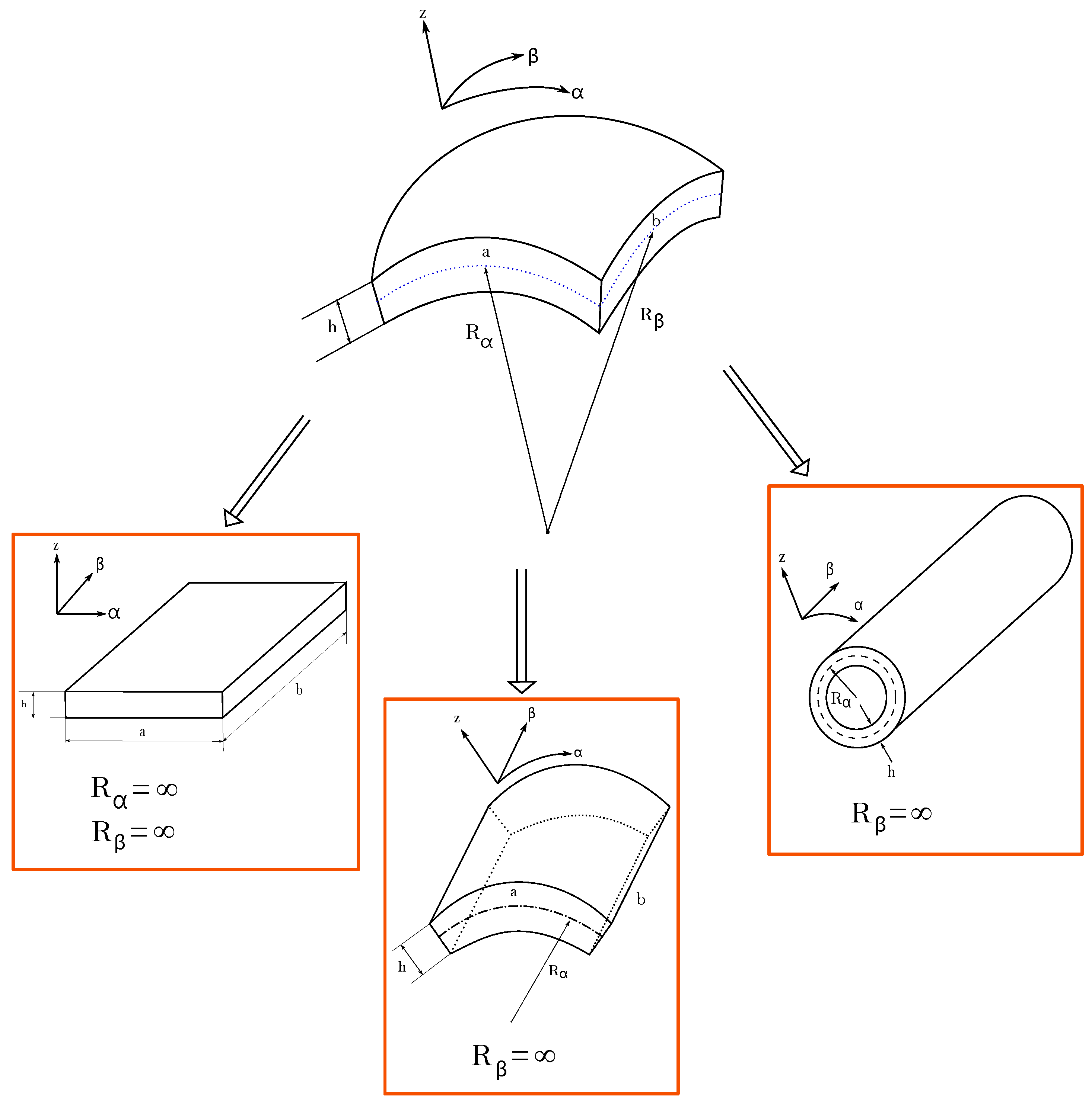
Here, four new benchmarks are proposed considering plates, cylinders, cylindrical shells, and spherical shells. The involved geometries can be seen in Figure 1. Several sovra-temperature impositions, different m and n half-wave numbers and different FGM laws are considered for each case. The variation of the FGM law occurs with the variation of the parameter p in the exponential law of Equation (45). For each possible geometry, a FGM layer is involved (both single-layer and sandwich configurations). In all the proposed 3D coupled results, the $N=3$ order of expansion for the exponential matrix and $M=300$ mathematical layers are used. The new 3D coupled exact thermo-elastic model (3D-u-$\theta$) will be used for these benchmarks and it will be compared with previously uncoupled 3D results where the 3D Fourier heat conduction equation was separately solved (3D(${\theta }_c$,3D)), the 1D Fourier heat conduction equation was separately solved (3D(${\theta }_c$,1D)), and the assumed linear temperature profiles were considered a priori (3D(${\theta }_a$)). The results presented in this subsection can be useful for those scientists involved in the development of 2D and 3D analytical and numerical models for the thermal stress analysis of plates and shells embedding FGM layers.

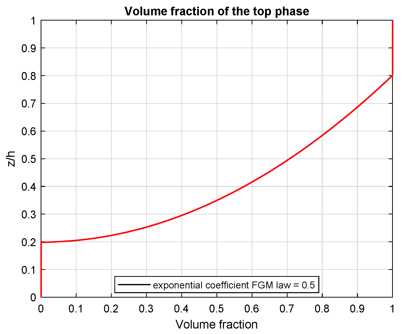
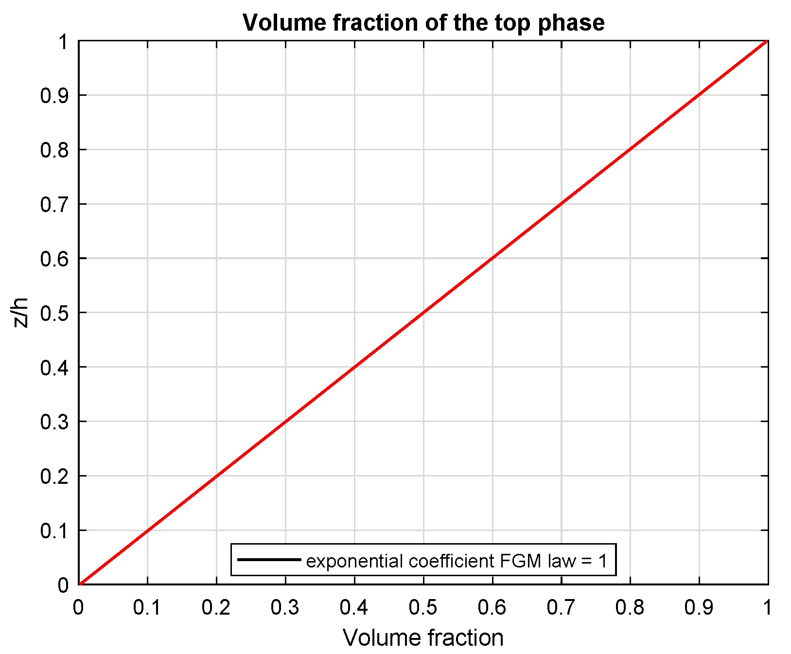
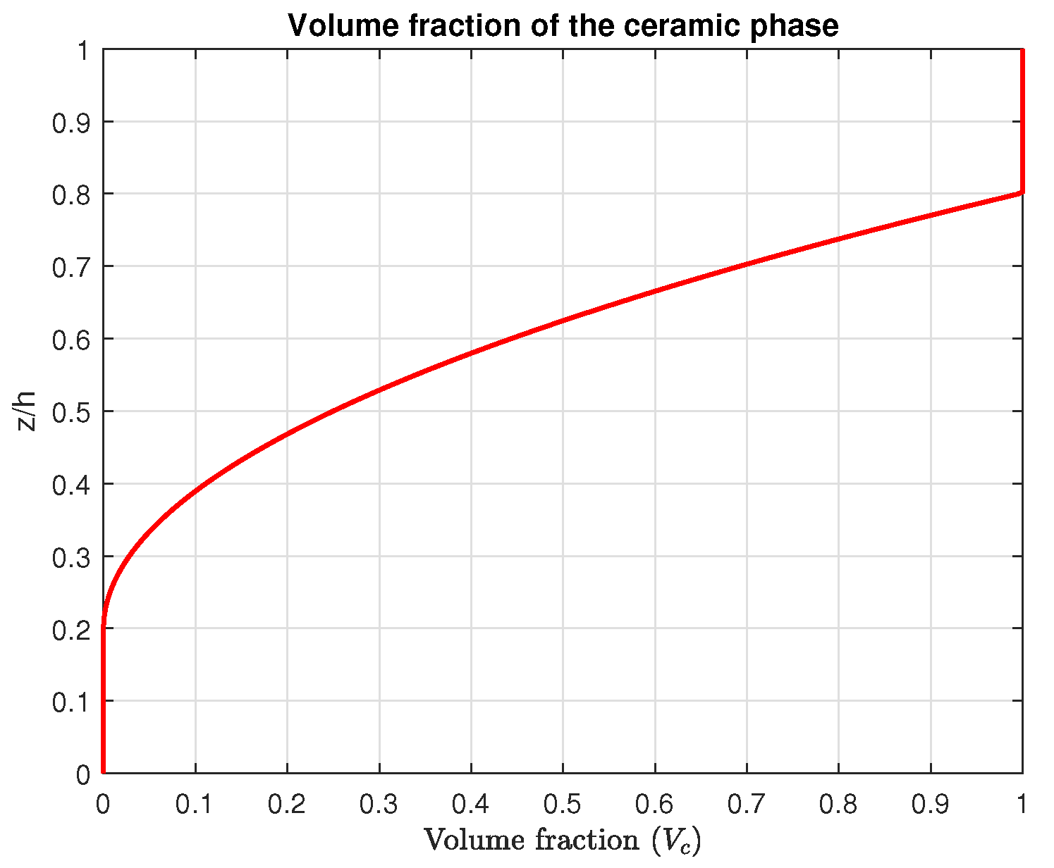
The first benchmark proposes a simply supported sandwich square plate ($a=b=10m$) with an FGM core (see Figure 1). The thickness of the entire structure is h and the analysed thickness ratios are $a/h=2,5,10,20,50,100$. The thickness of the top and bottom skins is $h_1=h_3=0.2h$ and the FGM core has $h_2=0.6h$. The sovra-temperature has an amplitude value at the top of ${\mathsf{\Theta }}_t=+0.5K$ and at the bottom ${\mathsf{\Theta }}_b=-0.5K$ with bi-sinusoidal form (half-wave numbers $m=1$ and $n=1$). The volume fraction law of the ceramic phase $V_c$ for the FGM core has exponential $p=2$; all the mechanical and thermal property variations of the FGM core through the thickness are described by means of Equations (46)–(48). The bottom skin is full metallic and the top skin is full ceramic, while the FGM core has a continuous variation (see Figure 2). 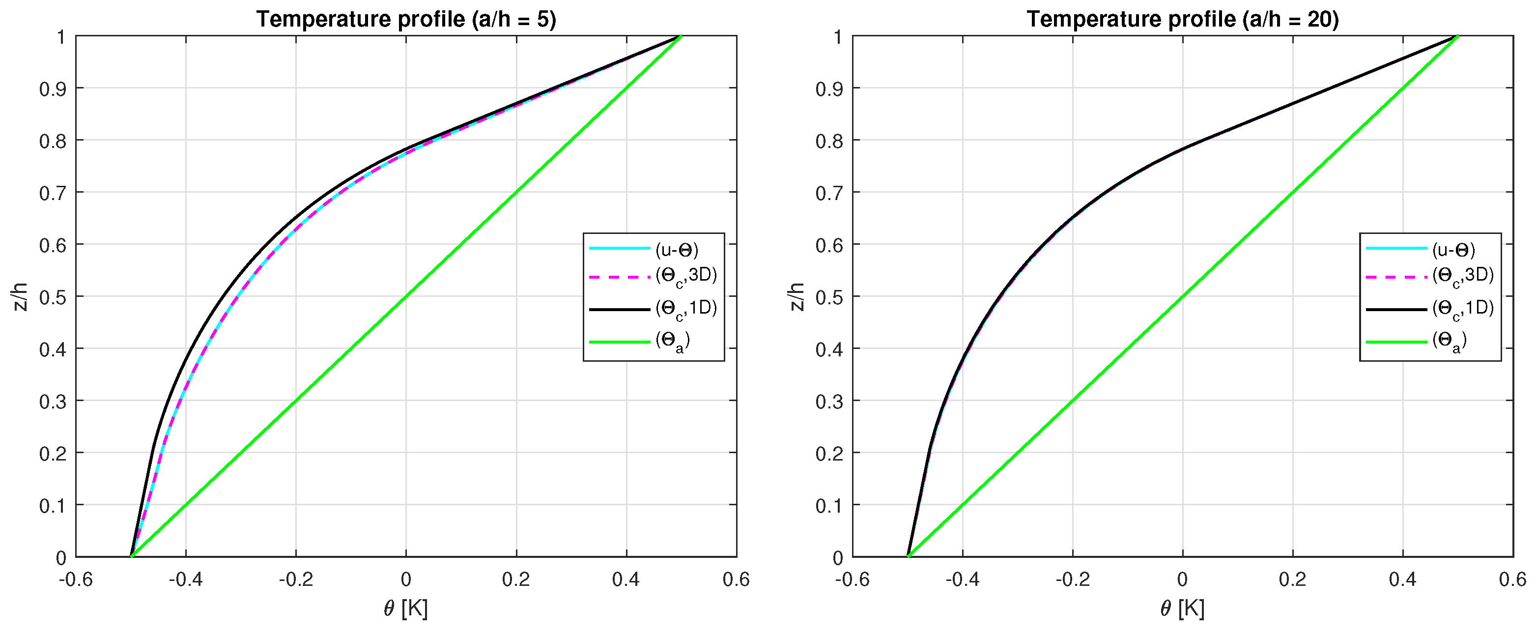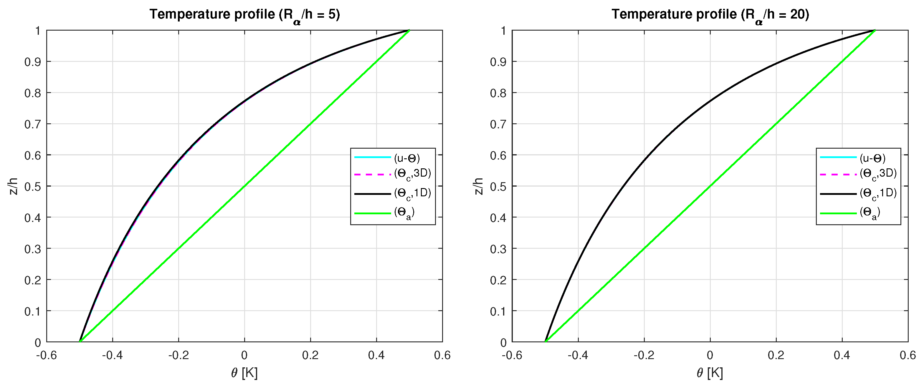Figure 3 shows the temperature profile through the thickness of a moderately thick ($a/h=5$) and a moderately thin ($a/h=20$) plate. In the case of the moderately thin configuration ($a/h=20$), the calculated temperature profiles using 3D Fourier heat conduction Equation (${\theta }_c$,3D), using 1D Fourier heat conduction Equation (${\theta }_c$,1D), and using the coupled model (u-$\theta$) are perfectly coincident. The assumed linear temperature profile (${\theta }_a$) is inappropriate for this case. For the moderately thick plate ($a/h=5$), the temperature profile calculated using the full coupled model (u-$\theta$) is coincident with the uncoupled model that computes the temperature profile via the 3D Fourier heat conduction Equation (${\theta }_c$,3D). These two models introduce both the thickness and material layer effects. The temperature profile using the 1D Fourier heat conduction Equation (${\theta }_c$,1D) does not consider the thickness layer effect. The uncoupled model that considers the temperature profile using an a priori linear assumption (${\theta }_a$) does not take into account both the effects.

Table 3. First benchmark, simply supported sandwich square plate with FGM (p = 0.5) core. Sovra-temperature imposed as ${\mathsf{\Theta }}_t=+0.5K$ and ${\mathsf{\Theta }}_b=-0.5K$ for $m=1$ and $n=1$. 3D uncoupled thermoelastic models from [70]. The new 3D coupled thermoelastic solution is 3D-u-$\theta$.

a/h	2	5	10	20	50	100
u[${10}^{-5}$ m] at ($\alpha =0$, $\beta =b/2$, $\overline{z}=0$)
3D(${\theta }_a$) [70]	1.6223	1.4866	1.4659	1.4606	1.4592	1.4589
3D(${\theta }_c$,1D) [70]	2.2351	2.0009	1.9613	1.9511	1.9482	1.9478
3D(${\theta }_c$,3D) [70]	1.9180	1.9463	1.9475	1.9477	1.9477	1.9477
3D-u-$\theta$	1.9180	1.9463	1.9475	1.9477	1.9477	1.9477
w[${10}^{-5}$ m] at ($\alpha =a/2$, $\beta =b/2$, $\overline{z}=h/2$)
3D(${\theta }_a$) [70]	1.4865	4.1617	8.4399	16.937	42.382	84.776
3D(${\theta }_c$,1D) [70]	1.4159	3.9997	8.1190	16.297	40.783	81.577
3D(${\theta }_c$,3D) [70]	1.3743	3.9724	8.1047	16.289	40.780	81.575
3D-u-$\theta$	1.3743	3.9724	8.1047	16.289	40.780	81.575
${\sigma }_{\beta \beta }$[${10}^3$ Pa] at ($\alpha =a/2$, $\beta =b/2$, $\overline{z}=h$)
3D(${\theta }_a$) [70]	−239.78	−258.49	−261.30	−262.01	−262.21	−262.24
3D(${\theta }_c$,1D) [70]	−731.19	−676.95	−665.61	−662.63	−661.78	−661.66
3D(${\theta }_c$,3D) [70]	−603.01	−652.62	−659.41	−661.07	−661.53	−661.60
3D-u-$\theta$	−603.01	−652.62	−659.41	−661.07	−661.53	−661.60
${\sigma }_{\alpha \beta }$[${10}^3$ Pa] at ($\alpha =0$, $\beta =0$, $\overline{z}=h/4$)
3D(${\theta }_a$) [70]	292.33	311.02	314.19	315.00	315.23	315.26
3D(${\theta }_c$,1D) [70]	498.38	515.05	518.41	519.29	519.54	519.58
3D(${\theta }_c$,3D) [70]	404.32	496.08	513.46	518.04	519.34	519.53
3D-u-$\theta$	404.32	496.08	513.46	518.04	519.34	519.53
${\sigma }_{\alpha z}$[${10}^3$ Pa] at ($\alpha =0$, $\beta =b/2$, $\overline{z}=h/4$)
3D(${\theta }_a$) [70]	−30.682	−17.013	−8.8995	−4.4999	−1.8056	−0.9032
3D(${\theta }_c$,1D) [70]	77.609	21.539	9.8156	4.7825	1.8988	0.9484
3D(${\theta }_c$,3D) [70]	37.694	18.520	9.4317	4.7343	1.8957	0.9480
3D-u-$\theta$	37.693	18.521	9.4317	4.7343	1.8957	0.9480
${\sigma }_{\beta z}$[${10}^3$ Pa] at ($\alpha =a/2$, $\beta =0$, $\overline{z}=3h/4$)
3D(${\theta }_a$) [70]	28.092	14.681	7.6209	3.8461	1.5424	0.7715
3D(${\theta }_c$,1D) [70]	−84.322	−25.702	−12.028	−5.9059	−2.3501	−1.1742
3D(${\theta }_c$,3D) [70]	−44.805	−22.672	−11.642	−5.8573	−2.3470	−1.1738
3D-u-$\theta$	−44.805	−22.672	−11.642	−5.8573	−2.3470	−1.1738
${\sigma }_{zz}$[${10}^3$ Pa] at ($\alpha =a/2$, $\beta =b/2$, $\overline{z}=3h/4$)
3D(${\theta }_a$) [70]	−17.007	−3.0277	−0.7695	−0.1932	−0.0310	−0.0077
3D(${\theta }_c$,1D) [70]	49.914	6.4569	1.5345	0.3784	0.0603	0.0151
3D(${\theta }_c$,3D) [70]	28.983	5.8135	1.4934	0.3758	0.0602	0.0151
3D-u-$\theta$	28.983	5.8135	1.4934	0.3758	0.0602	0.0151

shows the in-plane and transverse displacement components and the in-plane normal, in-plane shear, transverse shear, and transverse normal stress components in different positions through the thickness for different $a/h$ ratios. In the case of very thin plates ($a/h=100$), the last 3D models presented in Table 1 are coincident. For thick or moderately thick plates, the 3D(${\theta }_c$,3D) and the 3D-u-$\theta$ model provide the same results because they properly consider the thickness layer and material layer effects thanks to the implementation of the 3D Fourier heat conduction equation. The 3D(${\theta }_a$) model provides different results because it did not properly consider any material layer and thickness layer effect. 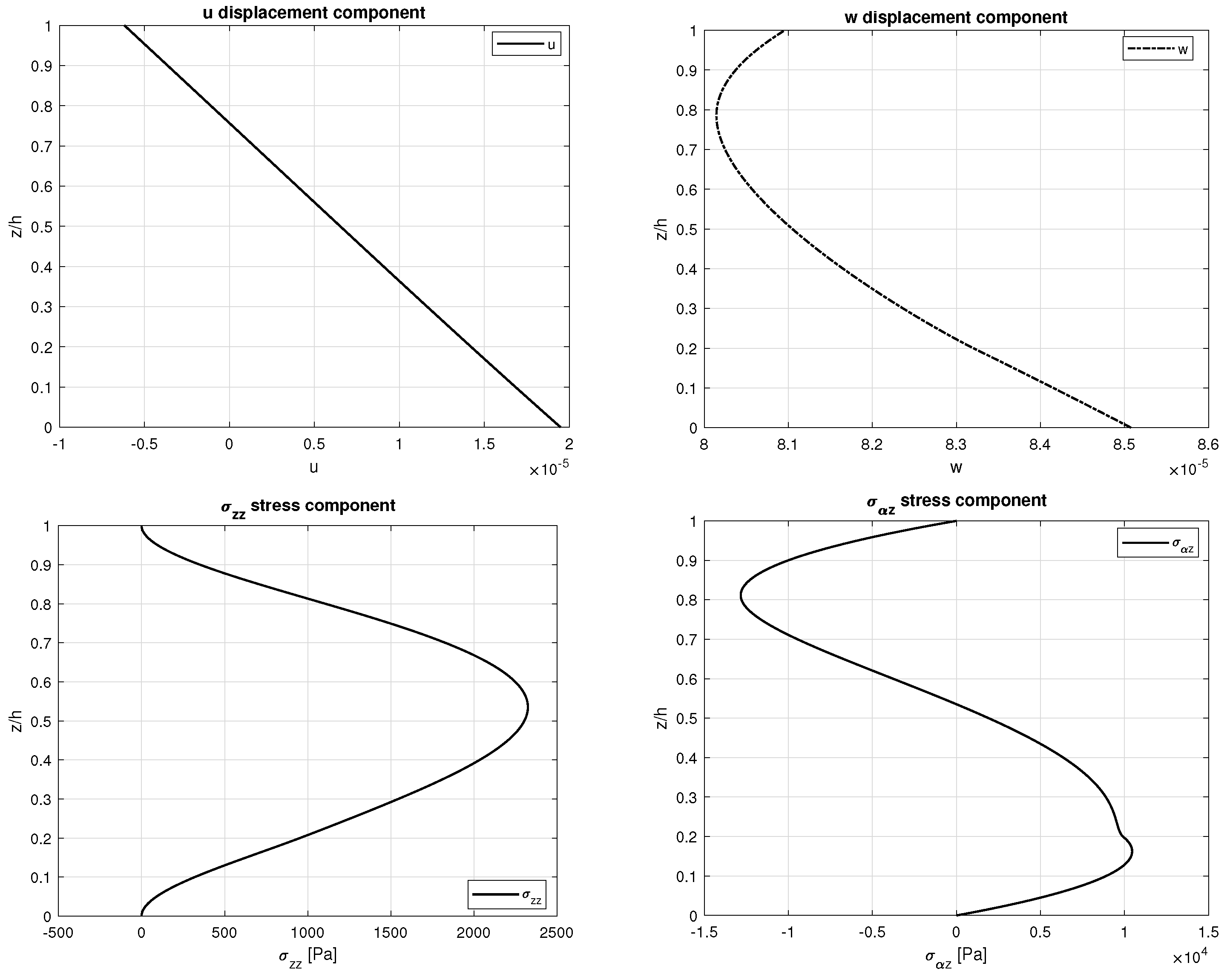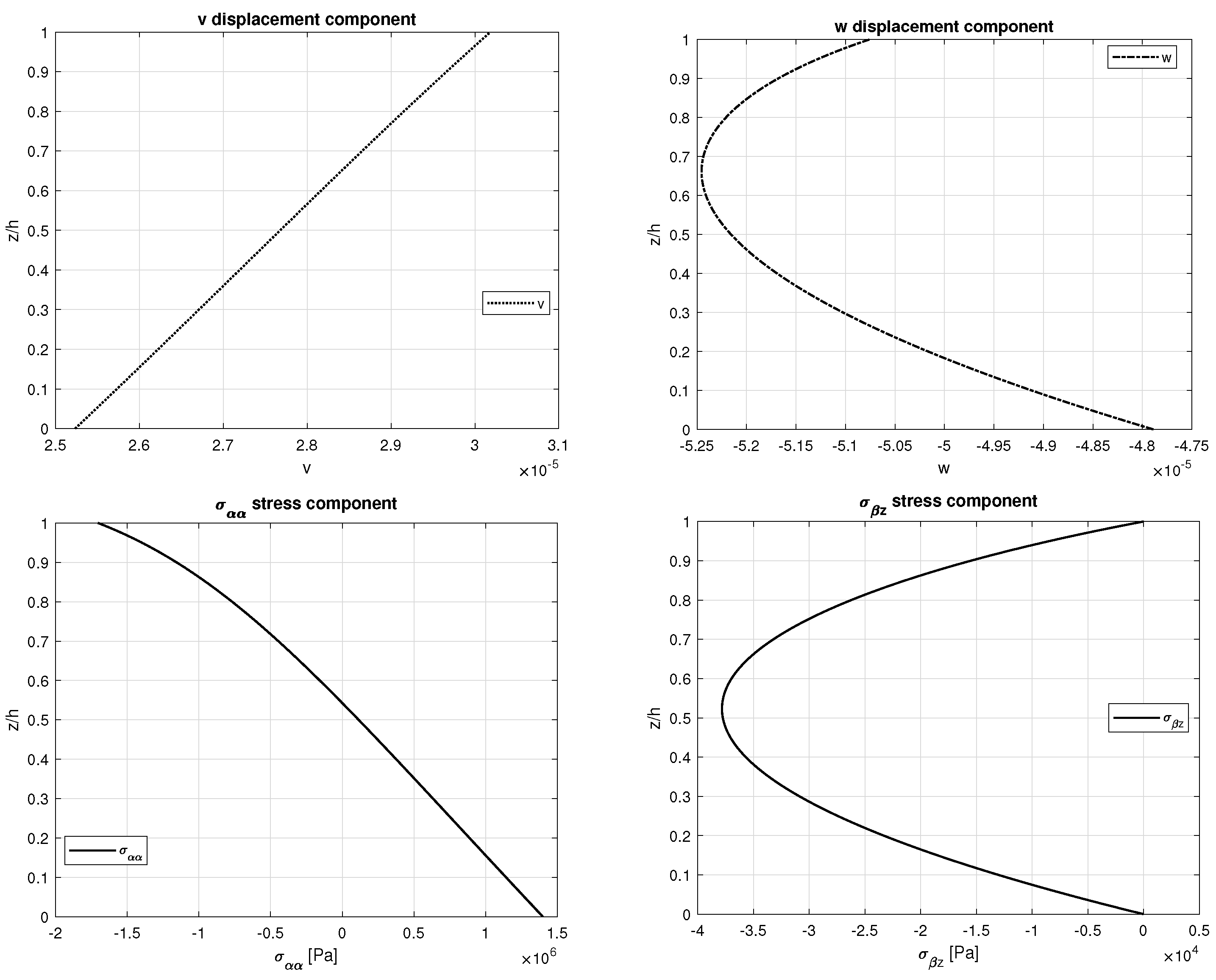Figure 4 shows the in-plane and transverse displacement components and two stress components (${\sigma }_{zz}$ and ${\sigma }_{\alpha z}$) through the thickness of a moderately thick plate ($a/h=10$). The in-plane displacement and transverse displacement are continuous through the thickness direction because the mechanical properties of the FGM layer vary with continuity along the thickness direction and the compatibility conditions are correctly introduced in the shell model. The transverse normal stress and the transverse shear stress satisfies the boundary load conditions imposed at the top and at the bottom external surfaces of the structures (${\sigma }_{zz}^t={\sigma }_{zz}^b=P_z=0$ and ${\sigma }_{\beta z}^t={\sigma }_{\beta z}^b=P_{\beta }=0$) and they are continuous because of the correct impositions of equilibrium conditions.

For the case related to the second benchmark, a simply supported one-layered FGM cylinder (see Figure 1) is analysed. The radii of curvature of the structure are $R_{\alpha }=10m$ and $R_{\beta }=\infty$. The global thickness of the structure is h. The in-plane dimensions are $a=2\pi R_{\alpha }$ and $b=30m$. The applied sovra-temperatures at the external surfaces are the same as those already proposed for the first benchmark, but half-wave numbers $m=2$ and $n=1$ are now imposed. The volume fraction of the ceramic phase $V_c$ is linear ($p=1$), the bottom of the structure is full metallic and the top is full ceramic as can be seen in Figure 5. The reference equations for all the material characteristics are proposed in Equations (46)–(48). The temperature profiles through the thickness proposed in Figure 6 do not change when the thickness ratio varies. This feature is due to the symmetry and rigidity of the cylinder. Therefore, the effect of the thickness is negligible even if the structure is really thick ($R_{\alpha }/h=5$ case).

Table 4. Second benchmark, simply supported cylinder with one FGM (p = 1) layer. Sovra-temperature imposed as ${\mathsf{\Theta }}_t=+0.5K$ and ${\mathsf{\Theta }}_b=-0.5K$ for $m=2$ and $n=1$. 3D uncoupled thermoelastic models from [70]. The new 3D coupled thermoelastic solution is 3D-u-$\theta$.

${\mathit{R}}_{\mathit{\alpha }}$/h	2	5	10	20	50	100
v[${10}^{-6}$ m] at ($\alpha =a/2$, $\beta =0$, $\overline{z}=h$)
3D(${\theta }_a$) [70]	−8.6733	2.8714	5.3717	6.2023	6.5527	6.6441
3D(${\theta }_c$,1D) [70]	24.724	30.279	30.248	29.774	29.340	29.170
3D(${\theta }_c$,3D) [70]	22.657	29.994	30.184	29.758	29.337	29.170
3D-u-$\theta$	22.657	29.994	30.184	29.758	29.337	29.170
w[${10}^{-5}$ m] at ($\alpha =a/2$, $\beta =b/2$, $\overline{z}=h/2$)
3D(${\theta }_a$) [70]	1.2362	−0.1105	−0.7159	−1.0306	−1.2201	−1.2831
3D(${\theta }_c$,1D) [70]	−2.9978	−4.6191	−5.2275	−5.5225	−5.6934	−5.7490
3D(${\theta }_c$,3D) [70]	−2.7332	−4.5726	−5.2158	−5.5196	−5.6929	−5.7489
3D-u-$\theta$	−2.7332	−4.5726	−5.2158	−5.5196	−5.6929	−5.7489
${\sigma }_{\alpha \alpha }$[${10}^3$ Pa] at ($\alpha =a/2$, $\beta =b/2$, $\overline{z}=0$)
3D(${\theta }_a$) [70]	2245.9	2104.6	2023.8	1977.7	1948.6	1938.6
3D(${\theta }_c$,1D) [70]	1802.3	1517.9	1396.1	1331.9	1292.8	1279.7
3D(${\theta }_c$,3D) [70]	1829.7	1523.9	1397.7	1332.4	1292.9	1279.7
3D-u-$\theta$	1829.7	1523.9	1397.7	1332.4	1292.9	1279.7
${\sigma }_{\alpha \beta }$[${10}^3$ Pa] at ($\alpha =0$, $\beta =0$, $\overline{z}=h/4$)
3D(${\theta }_a$) [70]	165.97	62.049	28.841	13.745	5.3213	2.6301
3D(${\theta }_c$,1D) [70]	143.90	44.761	19.011	8.5799	3.2023	1.5624
3D(${\theta }_c$,3D) [70]	143.38	44.833	19.024	8.5818	3.2025	1.5624
3D-u-$\theta$	143.38	44.833	19.024	8.5818	3.2025	1.5624
${\sigma }_{\alpha z}$[${10}^3$ Pa] at ($\alpha =0$, $\beta =b/2$, $\overline{z}=h/4$)
3D(${\theta }_a$) [70]	−177.52	−70.179	−34.135	−16.746	−6.6109	−3.2901
3D(${\theta }_c$,1D) [70]	−163.27	−57.830	−26.873	−12.859	−4.9976	−2.4739
3D(${\theta }_c$,3D) [70]	−162.57	−57.869	−26.881	−12.860	−4.9977	−2.4739
3D-u-$\theta$	−162.57	−57.869	−26.881	−12.860	−4.9977	−2.4739
${\sigma }_{\beta z}$[${10}^3$ Pa] at ($\alpha =a/2$, $\beta =0$, $\overline{z}=3h/4$)
3D(${\theta }_a$) [70]	−104.50	−52.635	−27.225	−13.710	−5.4896	−2.7442
3D(${\theta }_c$,1D) [70]	−142.28	−61.257	−30.160	−14.825	−5.8512	−2.9110
3D(${\theta }_c$,3D) [70]	−138.41	−61.063	−30.139	−14.823	−5.8511	−2.9110
3D-u-$\theta$	−138.41	−61.063	−30.139	−14.823	−5.8511	−2.9110
${\sigma }_{zz}$[${10}^3$ Pa] at ($\alpha =a/2$, $\beta =b/2$, $\overline{z}=3h/4$)
3D(${\theta }_a$) [70]	92.991	46.640	24.829	12.766	5.1869	2.6064
3D(${\theta }_c$,1D) [70]	118.96	53.212	27.251	13.742	5.5187	2.7624
3D(${\theta }_c$,3D) [70]	116.03	53.050	27.232	13.740	5.5186	2.7624
3D-u-$\theta$	116.03	53.050	27.232	13.740	5.5186	2.7624

shows the results in terms of displacements and stresses for different $R_{\alpha }/h$ ratios. For thicker cylinders, the 3D(${\theta }_c$,3D) and 3D-u-$\theta$ models are in accordance because they take into account both the material layer and the thickness layer effects. The 3D(${\theta }_c$,1D) only considers the material layer effect and 3D(${\theta }_a$) only considers a linear assumed temperature amplitude: for this reason, the results are not correct. For thin cylinders, only the 3D(${\theta }_a$) model shows important differences with respect to the other three models (3D(${\theta }_c$,1D), 3D(${\theta }_c$,3D), and 3D-u-$\theta$. Figure 7 provides the displacements and stresses for a moderately thick ($a/h=10$) cylinder with one FGM layer. In-plane and transverse displacements are continuous because the mechanical and thermal properties of the FGM layer vary continuously in the thickness direction and the compatibility conditions are correctly imposed for each mathematical interface. The same consideration is also valid for the stresses ${\sigma }_{\alpha \alpha }$ and ${\sigma }_{\beta z}$ shown in Figure 7. The transverse shear stress satisfies the free mechanical load conditions at the external surfaces (${\sigma }_{\beta z}^t={\sigma }_{\beta z}^b=P_{\beta }=0$).

The third benchmark presents a simply supported sandwich cylindrical shell with an FGM core (see Figure 1). The radii of curvature are $R_{\alpha }=10m$ and $R_{\beta }=\infty$ and the in-plane dimensions are $a=\frac{\pi }{3}{R}_{\alpha }$ and $b=30m$. The FGM core has thickness $h_2=0.6h$ and the two skins have $h_1=h_3=0.2h$; h is the global thickness of the structure. The material properties of this configuration are based on Equations (46)–(48) with a quadratic exponential coefficient ($p=2$). The bottom skin is full metallic and the top skin is full ceramic with thermal and mechanical properties expressed as in Equations (43) and (44) (as is visible in Figure 8). The investigated thickness ratios are $R_{\alpha }/h=2,5,10,20,50,100$. The sovra-temperature in harmonic form (half-wave numbers $m=1$ and $n=1$) has amplitude values at the top ${\mathsf{\Theta }}_t=-1K$ and at the bottom ${\mathsf{\Theta }}_b=0K$. The temperature profiles are provided in Figure 9 for a moderately thick ($R_{\alpha }/h=5$) and a moderately thin ($R_{\alpha }/h=20$) cylindrical shell. For thicker configurations, the thickness layer effect is a little bit more evident than the second benchmark because of the rigidity of the previous closed and symmetric cylinder. For thinner configurations, 3D(${\theta }_c$,1D), 3D(${\theta }_c$,3D), and 3D-u-$\theta$ models have no differences in terms of their temperature profiles. The 3D(${\theta }_a$) model always proposes an inadequate temperature profile because it did not consider any material layer and thickness layer effect. The same considerations are still valid for the discussion of displacements and stresses in

Table 5. Third benchmark, simply supported sandwich cylindrical shell with FGM (p = 2) core. Sovra-temperature imposed as ${\mathsf{\Theta }}_t=-1K$ and ${\mathsf{\Theta }}_b=0K$ for $m=1$ and $n=1$. 3D uncoupled thermoelastic models from [70]. The new 3D coupled thermoelastic solution is 3D-u-$\theta$.

${\mathit{R}}_{\mathit{\alpha }}$/h	2	5	10	20	50	100
u[${10}^{-5}$ m] at ($\alpha =0$, $\beta =b/2$, $\overline{z}=0$)
3D(${\theta }_a$) [70]	−0.1032	−2.5775	−6.5549	−13.028	−18.648	−18.423
3D(${\theta }_c$,1D) [70]	−1.0043	−2.5320	−4.8150	−8.0331	−9.7702	−8.8619
3D(${\theta }_c$,3D) [70]	−1.1076	−2.5335	−4.8060	−8.0263	−9.7682	−8.8613
3D-u-$\theta$	−1.1076	−2.5335	−4.8060	−8.0263	−9.7682	−8.8613
w[${10}^{-5}$ m] at ($\alpha =a/2$, $\beta =b/2$, $\overline{z}=h/2$)
3D(${\theta }_a$) [70]	−2.5005	−8.0358	−18.792	−37.833	−57.181	−58.624
3D(${\theta }_c$,1D) [70]	−2.0740	−5.8451	−12.332	−22.256	−29.339	−27.831
3D(${\theta }_c$,3D) [70]	−2.0327	−5.8020	−12.297	−22.235	−29.333	−27.829
3D-u-$\theta$	−2.0327	−5.8020	−12.297	−22.235	−29.333	−27.829
${\sigma }_{\beta \beta }$[${10}^3$ Pa] at ($\alpha =a/2$, $\beta =b/2$, $\overline{z}=h$)
3D(${\theta }_a$) [70]	1100.6	1034.2	823.07	553.81	506.00	655.96
3D(${\theta }_c$,1D) [70]	1521.1	1495.3	1395.3	1292.9	1352.4	1468.5
3D(${\theta }_c$,3D) [70]	1564.2	1504.9	1398.5	1293.9	1352.5	1468.6
3D-u-$\theta$	1564.2	1504.9	1398.5	1293.9	1352.5	1468.6
${\sigma }_{\alpha \beta }$[${10}^3$ Pa] at ($\alpha =0$, $\beta =0$, $\overline{z}=h/4$)
3D(${\theta }_a$) [70]	211.18	46.212	50.865	−66.576	−120.91	−83.255
3D(${\theta }_c$,1D) [70]	46.213	7.5615	−39.847	−90.780	−89.957	−55.402
3D(${\theta }_c$,3D) [70]	28.473	4.5755	−40.378	−90.820	−89.951	−55.400
3D-u-$\theta$	28.473	4.5755	−40.378	−90.820	−89.951	−55.400
${\sigma }_{\alpha z}$[${10}^3$ Pa] at ($\alpha =0$, $\beta =b/2$, $\overline{z}=h/4$)
3D(${\theta }_a$) [70]	23.813	−15.719	−17.016	−7.0833	5.0945	5.3470
3D(${\theta }_c$,1D) [70]	−79.295	−40.804	−21.620	−7.0251	2.5966	2.8247
3D(${\theta }_c$,3D) [70]	−89.122	−41.263	−21.634	−7.0233	2.5961	2.8246
3D-u-$\theta$	−89.122	−41.263	−21.634	−7.0233	2.5961	2.8246
${\sigma }_{\beta z}$[${10}^3$ Pa] at ($\alpha =a/2$, $\beta =0$, $\overline{z}=3h/4$)
3D(${\theta }_a$) [70]	−13.098	−15.405	−12.417	−6.3749	−0.1390	0.8218
3D(${\theta }_c$,1D) [70]	29.138	7.4634	2.3569	2.0687	2.5041	1.7405
3D(${\theta }_c$,3D) [70]	32.873	7.8962	2.4322	2.0798	2.5046	1.7406
3D-u-$\theta$	32.873	7.8962	2.4322	2.0798	2.5046	1.7406
${\sigma }_{zz}$[${10}^3$ Pa] at ($\alpha =a/2$, $\beta =b/2$, $\overline{z}=3h/4$)
3D(${\theta }_a$) [70]	42.679	16.454	10.492	5.0412	−0.1093	−0.8396
3D(${\theta }_c$,1D) [70]	−40.599	−11.996	−4.5234	−2.8784	−2.5498	−1.6952
3D(${\theta }_c$,3D) [70]	−48.215	−12.534	−4.5992	−2.8887	−2.5503	−1.6952
3D-u-$\theta$	−48.215	−12.534	−4.5992	−2.8887	−2.5503	−1.6952

where the 3D(${\theta }_c$,1D), 3D(${\theta }_c$,3D), and 3D-u-$\theta$ models are quite coincident for all the $R_{\alpha }/h$ ratios proposed. The great difference involves only the 3D(${\theta }_a$) model that is always inadequate for this configuration. Figure 10 shows displacement and stress evaluations through the thickness of the simply supported sandwich cylindrical shell with an FGM core. The analysed cylindrical shell is moderately thick and both proposed displacements and stresses are continuous because the FGM properties continuously vary along the thickness direction.

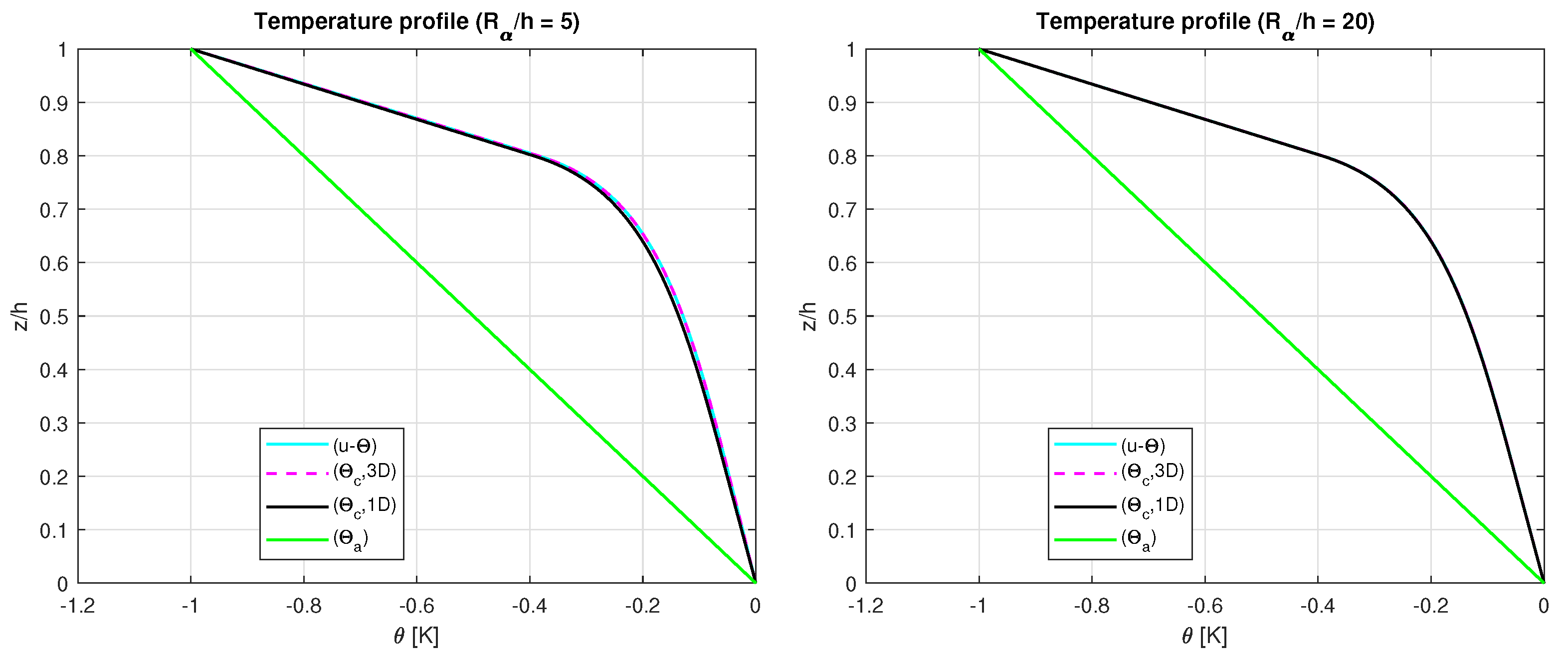
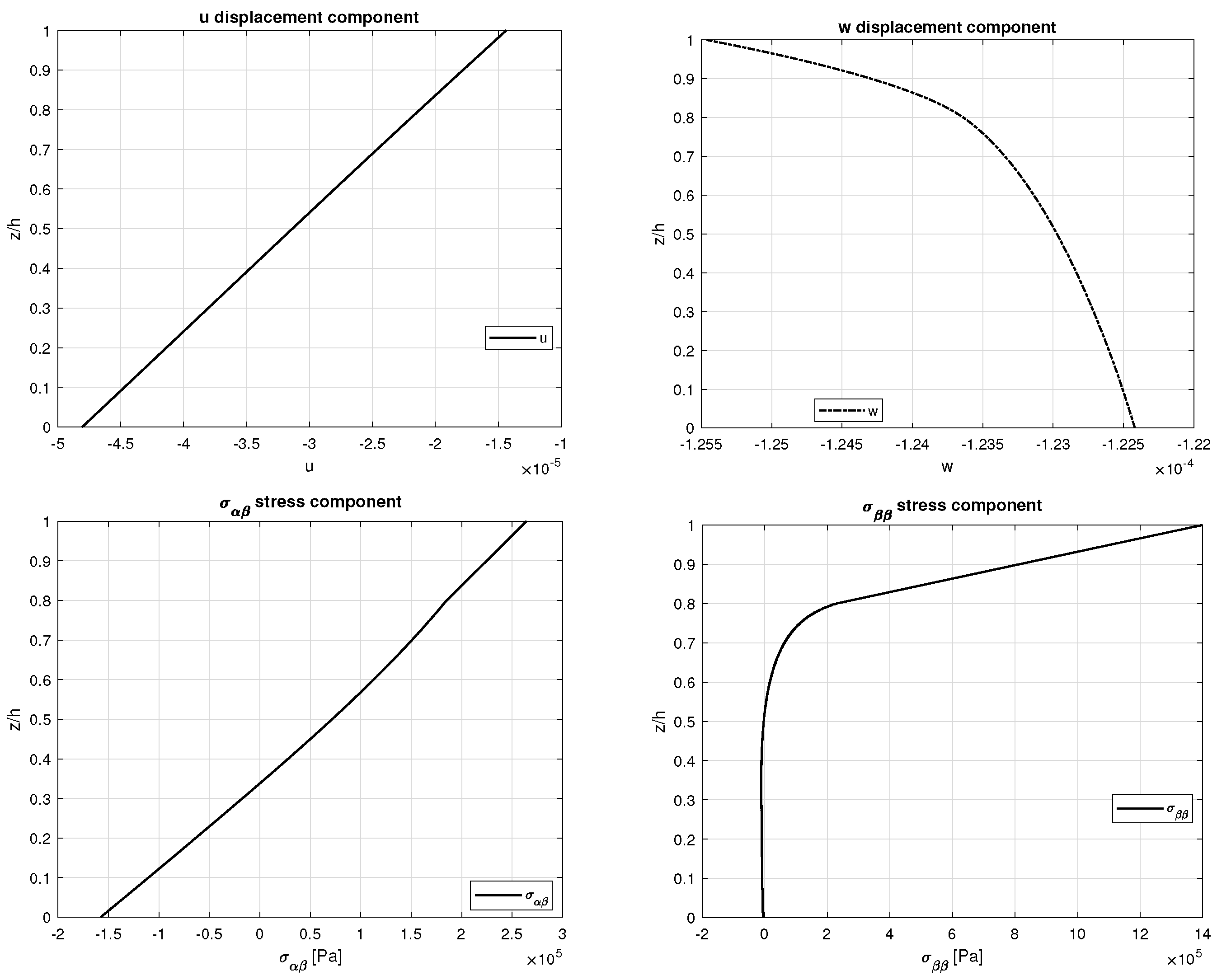
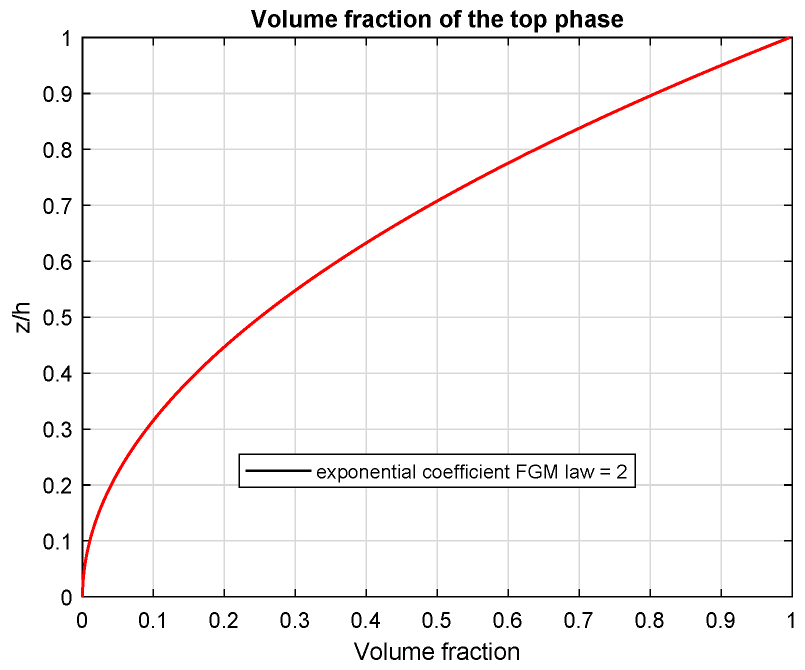
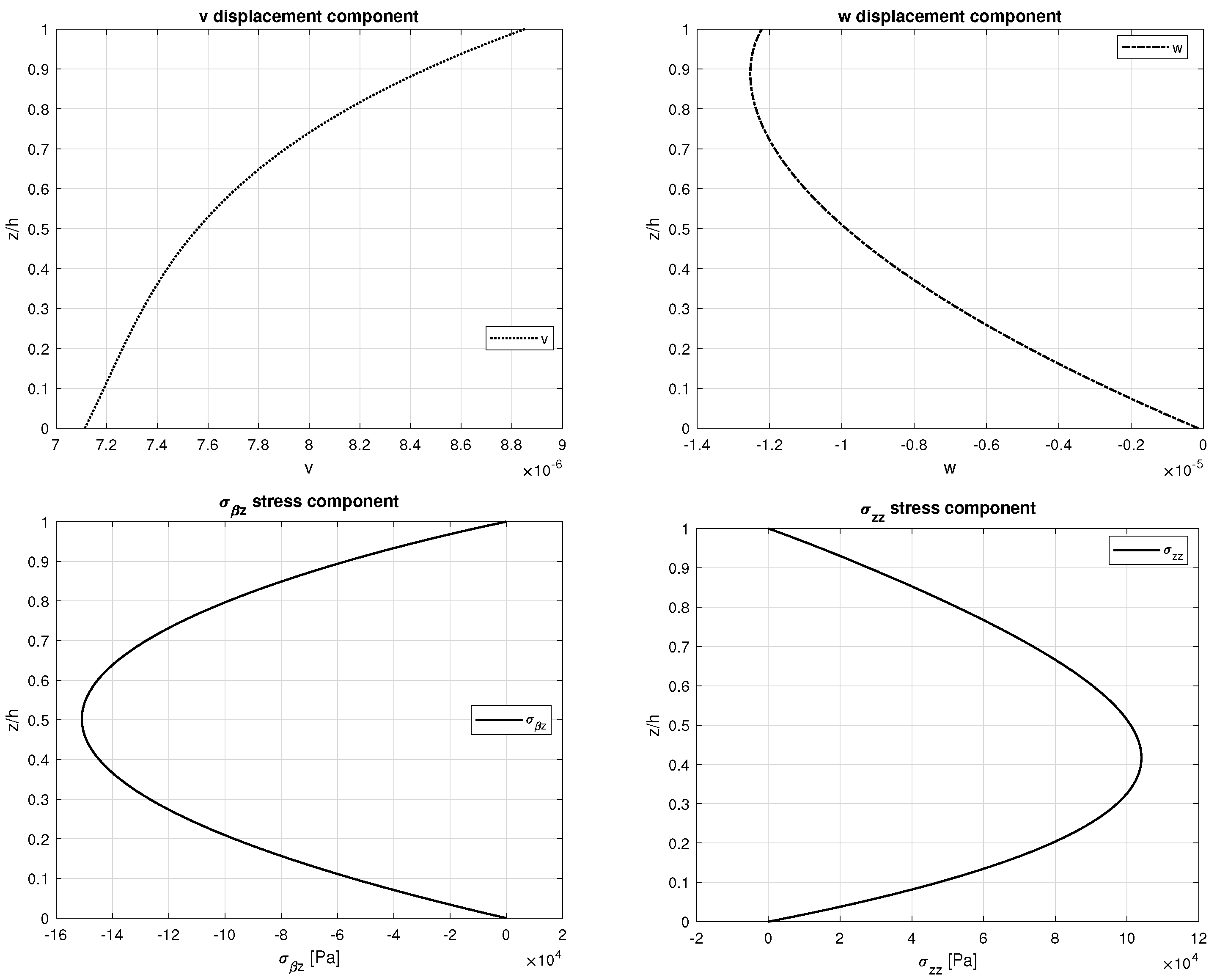
The last benchmark takes into account a simply supported spherical shell with one FGM layer (see Figure 1). The global thickness is h, the radii of curvature are $R_{\alpha }=R_{\beta }=10m$, the imposed sovra-temperatures are ${\mathsf{\Theta }}_t=0K$ and ${\mathsf{\Theta }}_b=-1K$, the in-plane dimensions are $a=\frac{\pi }{3}{R}_{\alpha }=b=\frac{\pi }{3}{R}_{\beta }$, and the half-wave numbers are $m=2$ and $n=1$. The configuration and material characteristics are the same as seen in the second benchmark (see Equations (46)–(48) for the bulk modulus, shear modulus, thermal expansion coefficient, and conductivity coefficient and see Equation (45) and Figure 11 for the volume fraction of the ceramic phase $V_c$ with $p=2$). In Figure 12, the temperature profile for the four models are shown. The 3D(${\theta }_c$,3D) and 3D-u-$\theta$ models are mandatory for the correct analysis of the thick shells. The 3D(${\theta }_c$,1D) model is a good approximation only for thin spherical shells, but it always denotes some differences with respect to the previous two models. The 3D(${\theta }_a$) model is always inappropriate for this benchmark for each $R_{\alpha }/h$ ratio considered. For the spherical shell, the thick configuration shows an important thickness layer effect. As in the previous benchmark, the 3D-u-$\theta$ model provides the same results obtained with the 3D(${\theta }_c$,3D) model because they consider both the thickness layer and the material layer effects. The displacements and stresses for several $R_{\alpha }/h$ are proposed in

Table 6. Fourth benchmark, simply supported spherical shell with one FGM (p = 2) layer. Sovra-temperature imposed as ${\mathsf{\Theta }}_t=0K$ and ${\mathsf{\Theta }}_b=-1K$ for $m=2$ and $n=1$. 3D uncoupled thermoelastic models from [70]. The new 3D coupled thermoelastic solution is 3D-u-$\theta$.

${\mathit{R}}_{\mathit{\alpha }}$/h	2	5	10	20	50	100
v[${10}^{-6}$ m] at ($\alpha =a/2$, $\beta =0$, $\overline{z}=h$)
3D(${\theta }_a$) [70]	3.8133	4.3442	6.2723	6.3118	3.4996	1.8525
3D(${\theta }_c$,1D) [70]	8.1671	8.0198	9.3872	8.2942	4.2336	2.1785
3D(${\theta }_c$,3D) [70]	1.5635	6.0279	8.8526	8.1968	4.2271	2.1778
3D-u-$\theta$	1.5635	6.0279	8.8526	8.1968	4.2271	2.1778
w[${10}^{-5}$ m] at ($\alpha =a/2$, $\beta =b/2$, $\overline{z}=h/2$)
3D(${\theta }_a$) [70]	−0.0045	0.7679	0.1533	−2.3272	−5.4440	−6.5416
3D(${\theta }_c$,1D) [70]	−0.2283	0.1565	−1.1720	−4.4728	−8.0033	−9.1116
3D(${\theta }_c$,3D) [70]	0.1726	0.4099	−0.9875	−4.3848	−7.9847	−9.1067
3D-u-$\theta$	0.1726	0.4099	−0.9875	−4.3848	−7.9847	−9.1067
${\sigma }_{\alpha \alpha }$[${10}^3$ Pa] at ($\alpha =a/2$, $\beta =b/2$, $\overline{z}=0$)
3D(${\theta }_a$) [70]	−627.94	1354.3	2306.7	2822.4	2666.3	2442.3
3D(${\theta }_c$,1D) [70]	−1140.7	1156.2	2169.3	2555.0	2157.7	1832.7
3D(${\theta }_c$,3D) [70]	797.05	1425.5	2219.4	2570.5	2161.7	1833.9
3D-u-$\theta$	797.11	1425.5	2219.4	2570.5	2161.7	1833.9
${\sigma }_{\alpha \beta }$[${10}^3$ Pa] at ($\alpha =0$, $\beta =0$, $\overline{z}=h/4$)
3D(${\theta }_a$) [70]	827.55	754.23	583.00	310.60	85.349	30.478
3D(${\theta }_c$,1D) [70]	981.89	833.16	595.79	276.15	52.204	10.609
3D(${\theta }_c$,3D) [70]	500.42	747.63	584.62	276.18	52.348	10.634
3D-u-$\theta$	500.41	747.63	584.62	276.18	52.348	10.634
${\sigma }_{\alpha z}$[${10}^3$ Pa] at ($\alpha =0$, $\beta =b/2$, $\overline{z}=h/4$)
3D(${\theta }_a$) [70]	21.383	−227.08	−223.11	−149.47	−58.821	−27.092
3D(${\theta }_c$,1D) [70]	149.49	−219.90	−228.25	−145.56	−51.490	−22.143
3D(${\theta }_c$,3D) [70]	−125.09	−225.85	−226.36	−145.42	−51.517	−22.149
3D-u-$\theta$	−125.09	−225.84	−226.36	−145.42	−51.517	−22.149
${\sigma }_{\beta z}$[${10}^3$ Pa] at ($\alpha =a/2$, $\beta =0$, $\overline{z}=3h/4$)
3D(${\theta }_a$) [70]	−184.45	−104.69	−91.933	−63.362	−25.499	−11.800
3D(${\theta }_c$,1D) [70]	−296.96	−158.20	−121.36	−75.344	−27.707	−12.309
3D(${\theta }_c$,3D) [70]	−60.985	−120.11	−114.83	−74.530	−27.670	−12.306
3D-u-$\theta$	−60.984	−120.11	−114.83	−74.530	−27.670	−12.306
${\sigma }_{zz}$[${10}^3$ Pa] at ($\alpha =a/2$, $\beta =b/2$, $\overline{z}=3h/4$)
3D(${\theta }_a$) [70]	237.90	70.115	51.648	35.425	15.234	7.3766
3D(${\theta }_c$,1D) [70]	391.90	107.16	67.497	41.558	16.381	7.6416
3D(${\theta }_c$,3D) [70]	73.490	79.064	63.665	41.100	16.360	7.6394
3D-u-$\theta$	73.490	79.064	63.665	41.100	16.360	7.6394

where it is evident how the results obtained using the 3D(${\theta }_a$) model are inadequate for each thickness ratio because the actual temperature profile is never linear along the thickness direction. In Figure 13, the displacement and stress evaluations through the thickness of a spherical shell with one FGM layer are shown. In-plane and transverse displacements, transverse shear, and transverse normal stress are continuous because the compatibility and equilibrium conditions have been correctly imposed and also because the FGM layer continuously varies its own mechanical and thermal properties along the thickness direction. Transverse normal stress ${\sigma }_{zz}$ satisfies the load boundary conditions (${\sigma }_{zz}^t={\sigma }_{zz}^b=P_z=0$) as can be seen in Figure 13.

4. Conclusions

A full coupled thermo-elastic 3D exact shell solution for thermal stress analysis of shells and plates embedding FGM layers has been proposed. The sovra-temperature amplitudes have been directly imposed at the external surfaces in steady-state conditions and the sovra-temperature profile was evaluated along the z direction. The sovra-temperature profile is a primary unknown variable similar to the displacements; this is possible because the 3D Fourier heat conduction equation and the 3D equilibrium equations for shells are put together into a set of four second-order differential equations. This temperature profile considers both the thickness layer and material layer effects for each possible geometry, without separately solving the related 3D Fourier heat conduction equation. The set of four second-order differential equations for shells is solved in a closed-form thanks to the Navier solution and the exponential matrix method. Different analyses, in terms of displacements, temperature profiles, in-plane, and out-of-plane stresses have been shown for several thickness ratios, geometries, FGM configurations, and temperature impositions. The proposed results showed a complete match between the model that separately solves the 3D Fourier heat conduction equation and the present 3D full coupled thermo-elastic model. For each investigated variable (temperatures, displacements and stresses) and for each thickness ratio, geometry, FGM configuration, and load imposition, the results proposed differences that were always less than 0.5%. This new coupled method permits taking into account both the material and the thickness layer effects using a simpler and more consistent mathematical formulation. Moreover, a reduced number of fictitious layers M is requested in comparison with the uncoupled 3D model; this feature permits having the same accurate results for a less complicated fictitious layer discretization.

References

1. Librescu, L.; Marzocca, P. Thermal Stresses ’03, Vol. 1; Virginia Polytechnic Institute and State University: Blacksburg, VA, USA, 2003. [Google Scholar]
2. Librescu, L.; Marzocca, P. Thermal Stresses ’03, Vol. 2; Virginia Polytechnic Institute and State University: Blacksburg, VA, USA, 2003. [Google Scholar]
3. Nowinski, J.L. Theory of Thermoelasticity with Applications; Sijthoff & Noordhoff: Alphen aan den Rijn, The Netherlands, 1978. [Google Scholar]
4. Noor, A.K.; Burton, W.S. Computational models for high-temperature multilayered composite plates and shells. Appl. Mech. Rev. 1992, 45, 419–446. [Google Scholar] [CrossRef]
5. Swaminathan, K.; Sangeetha, D.M. Thermal analysis of FGM plates—A critical review of various modeling techniques and solution methods. Compos. Struct. 2017, 160, 43–60. [Google Scholar] [CrossRef]
6. Altay, G.A.; Dökmeci, M.C. Fundamental variational equations of discontinuous thermopiezoelectric fields. Int. J. Eng. Sci. 1996, 34, 769–782. [Google Scholar] [CrossRef]
7. Altay, G.A.; Dökmeci, M.C. Some variational principles for linear coupled thermoelasticity. Int. J. Solids Struct. 1996, 33, 3937–3948. [Google Scholar] [CrossRef]
8. Altay, G.A.; Dökmeci, M.C. Coupled thermoelastic shell equations with second sound for high-frequency vibrations of temperature-dependent materials. Int. J. Solids Struct. 2001, 38, 2737–2768. [Google Scholar] [CrossRef]
9. Cannarozzi, A.A.; Ubertini, F. A mixed variational method for linear coupled thermoelastic analysis. Int. J. Solids Struct. 2001, 38, 717–739. [Google Scholar] [CrossRef]
10. Das, N.C.; Das, S.N.; Das, B. Eigenvalue approach to thermoelasticity. J. Therm. Stress. 1983, 6, 35–43. [Google Scholar] [CrossRef]
11. Kosìnski, W.; Frischmuth, K. Thermomechanical coupled waves in a nonlinear medium. Wave Motion 2001, 34, 131–141. [Google Scholar] [CrossRef]
12. Wauer, J. Free and forced magneto-thermo-elastic vibrations in a conducting plate layer. J. Therm. Stress. 1996, 19, 671–691. [Google Scholar] [CrossRef]
13. Kapuria, S.; Bhattacharyya, M.; Kumar, A.N. Bending and free vibration response of layered functionally graded beams: A theoretical model and its experimental validation. Compos. Struct. 2007, 82, 390–402. [Google Scholar] [CrossRef]
14. Kiani, Y.; Eslami, M.R. Thermal buckling analysis of functionally graded material beams. Int. J. Mech. Mater. Des. 2010, 6, 229–238. [Google Scholar] [CrossRef]
15. Ghiasian, S.E.; Kiani, Y.; Eslami, M.R. Dynamic buckling of suddenly heated or compressed FGM beams resting on nonlinear elastic foundation. Compos. Struct. 2013, 106, 225–234. [Google Scholar] [CrossRef]
16. Sun, Y.; Li, S.-R.; Batra, R.C. Thermal buckling and post-buckling of FGM Timoshenko beams on nonlinear elastic foundation. J. Therm. Stress. 2016, 39, 11–26. [Google Scholar] [CrossRef] [Green Version]
17. Ma, L.S.; Lee, D.W. Exact solutions for nonlinear static responses of a shear deformable FGM beam under an in-plane thermal loading. Eur. J. Mech. A/Solids 2012, 31, 13–20. [Google Scholar] [CrossRef]
18. Paul, A.; Das, D. Non-linear thermal post-buckling analysis of FGM Timoshenko beam under non-uniform temperature rise across thickness. Eng. Sci. Technol. Int. J. 2016, 19, 1608–1625. [Google Scholar] [CrossRef] [Green Version]
19. Zhang, J.; Chen, L.; Lv, Y. Elastoplastic thermal buckling of functionally graded material beams. Compos. Struct. 2019, 224, 111014. [Google Scholar] [CrossRef]
20. Chakraborty, A.; Gopalakrishnana, S.; Reddy, J.N. A new beam finite element for the analysis of functionally graded materials. Int. J. Mech. Sci. 2003, 45, 519–539. [Google Scholar] [CrossRef]
21. Chen, Y.; Jin, G.; Zhang, C.; Ye, T.; Xue, Y. Thermal vibration of FGM beams with general boundary conditions using a higher-order shear deformation theory. Compos. Part B 2018, 153, 376–386. [Google Scholar] [CrossRef]
22. Esen, I. Dynamic response of functional graded Timoshenko beams in a thermal environment subjected to an accelerating load. Eur. J. Mech. A/Solids 2019, 78, 103841. [Google Scholar] [CrossRef]
23. Esfahani, S.E.; Kiani, Y.; Eslami, M.R. Non-linear thermal stability analysis of temperature dependent FGM beams supported on non-linear hardening elastic foundations. Int. J. Mech. Sci. 2013, 69, 10–20. [Google Scholar] [CrossRef]
24. Li, Y.; Tang, Y. Application of Galerkin iterative technique to nonlinear bending response of three-directional functionally graded slender beams subjected to hygro-thermal loads. Compos. Struct. 2022, 290, 115481. [Google Scholar] [CrossRef]
25. Şimşek, M. Buckling of Timoshenko beams composed of two-dimensional functionally graded material (2D-FGM) having different boundary conditions. Compos. Struct. 2016, 149, 304–314. [Google Scholar] [CrossRef]
26. Ziane, N.; Meftah, S.A.; Ruta, G.; Tounsi, A. Thermal effects on the instabilities of porous FGM box beams. Eng. Struct. 2017, 134, 150–158. [Google Scholar] [CrossRef]
27. Javaheri, R.; Eslami, M.R. Thermal buckling of functionally graded plates based on higher order theory. J. Therm. Stress. 2002, 25, 603–625. [Google Scholar] [CrossRef]
28. Akbaş, S.D. Vibration and static analysis of functionally graded porous plates. J. Appl. Comput. Mech. 2017, 3, 199–207. [Google Scholar]
29. Saad, M.; Hadji, L. Thermal buckling analysis of porous FGM plates. Mater. Today Proc. 2022, 53, 196–201. [Google Scholar] [CrossRef]
30. Sangeetha, D.M.; Naveenkumar, D.T.; Vınaykuma, V.; Prakash, K.E. Temperature stresses in Functionally graded (FGM) material plates using deformation theory—Analytical approach. Mater. Today Proc. 2022, 49, 1936–1941. [Google Scholar] [CrossRef]
31. Zenkour, A.M.; Mashat, D.S. Thermal buckling analysis of ceramic-metal functionally graded plates. Nat. Sci. 2010, 2, 968–978. [Google Scholar] [CrossRef]
32. Yaghoobi, M.P.; Ghannad, M. An analytical solution for heat conduction of FGM cylinders with varying thickness subjected to non-uniform heat flux using a first-order temperature theory and perturbation technique. Int. Commun. Heat Mass Transf. 2020, 116, 104684. [Google Scholar] [CrossRef]
33. Zeighami, V.; Jafari, M. A closed-form solution for thermoelastic stress analysis of perforated asymmetric functionally graded nanocomposite plates. Theor. Appl. Fract. Mech. 2022, 118, 103251. [Google Scholar] [CrossRef]
34. Praveen, G.N.; Reddy, J.N. Nonlinear transient thermoelastic analysis of functionally graded ceramic-metal plates. Int. J. Solid Strcut. 1998, 35, 4457–4476. [Google Scholar] [CrossRef]
35. Thai, C.H.; Zenkour, A.M.; Wahab, M.A.; Nguyen-Xuan, H. A simple four-unknown shear and normal deformations theory for functionally graded isotropic and sandwich plates based on isogeometric analysis. Compos. Struct. 2016, 139, 77–95. [Google Scholar] [CrossRef]
36. Parandvar, H.; Farid, M. Large amplitude vibration of FGM plates in thermal environment subjected to simultaneously static pressure and harmonic force using multimodal FEM. Compos. Struct. 2016, 141, 163–171. [Google Scholar] [CrossRef]
37. Cho, J.R.; Oden, J.T. Functionally graded material: A parametric study on thermal-stress characteristics using the Crank-Nicolson-Galerkin scheme. Comput. Methods Appl. Mech. Eng. 2000, 188, 17–38. [Google Scholar] [CrossRef]
38. Alibeigloo, A. Thermo elasticity solution of sandwich circular plate with functionally graded core using generalized differential quadrature method. Compos. Struct. 2016, 136, 229–240. [Google Scholar] [CrossRef]
39. Hong, C.C. GDQ computation for thermal vibration of thick FGM plates by using fully homogeneous equation and TSDT. Thin-Walled Struct. 2019, 135, 78–88. [Google Scholar] [CrossRef]
40. Karakoti, A.; Pandey, S.; Kar, V.R. Nonlinear transient analysis of porous P-FGM and S-FGM sandwich plates and shell panels under blast loading and thermal environment. Thin-Walled Struct. 2022, 173, 108985. [Google Scholar] [CrossRef]
41. Jooybar, N.; Malekzadeh, P.; Fiouz, A.; Vaghefi, M. Thermal effect on free vibration of functionally graded truncated conical shell panels. Thin-Walled Struct. 2016, 103, 45–61. [Google Scholar] [CrossRef]
42. Tao, C.; Dai, T. Analyses of thermal buckling and secondary instability of post-buckled S-FGM plates with porosities based on a meshfree method. Appl. Math. Model. 2021, 89, 268–284. [Google Scholar] [CrossRef]
43. Qi, Y.-N.; Dai, H.-L.; Deng, S.-T. Thermoelastic analysis of stiffened sandwich doubly curved plate with FGM core under low velocity impact. Compos. Struct. 2020, 253, 112826. [Google Scholar] [CrossRef]
44. Gulshan Taj, M.N.A.; Chakrabarti, A.; Sheikh, A.H. Analysis of functionally graded plates using higher order shear deformation theory. Appl. Math. Model. 2013, 37, 8484–8494. [Google Scholar] [CrossRef]
45. Reddy, J.N.; Cheng, Z.-Q. Three-dimensional solutions of smart functionally graded plates. J. Appl. Mech. 2001, 68, 234–241. [Google Scholar] [CrossRef]
46. Jiang, H.-J.; Dai, H.-L. Analytical solutions for three-dimensional steady and transient heat conduction problems of a double-layer plate with a local heat source. Int. J. Heat Mass Transf. 2015, 89, 652–666. [Google Scholar] [CrossRef]
47. Chen, W.-Q.; Bian, Z.-G.; Ding, H.-J. Three-dimensional analysis of a thick FGM rectangular plate in thermal environment. Int. Zhejiang Univ. Sci. A 2003, 4, 1–7. [Google Scholar] [CrossRef]
48. Ootao, Y.; Tanigawa, Y. Three-dimensional solution for transient thermal stresses of an orthotropic functionally graded rectangular plate. Compos. Struct. 2007, 80, 10–20. [Google Scholar] [CrossRef]
49. Ootao, Y.; Tanigawa, Y. Three-dimensional transient thermal stresses of functionally graded rectangular plate due to partial heating. J. Therm. Stress. 2010, 22, 35–55. [Google Scholar]
50. Jabbari, M.; Shahryari, E.; Haghighat, H.; Eslami, M.R. An analytical solution for steady state three dimensional thermoelasticity of functionally graded circular plates due to axisymmetric loads. Eur. J. Mech. A/Solids 2014, 47, 124–142. [Google Scholar] [CrossRef]
51. Vel, S.S.; Batra, R.C. Exact solution for thermoelastic deformations of functionally graded thick rectangular plates. AIAA J. 2002, 40, 1421–1433. [Google Scholar] [CrossRef]
52. Liu, W.-X. Analysis of steady heat conduction for 3D axisymmetric functionally graded circular plate. J. Cent. South Univ. 2013, 20, 1616–1622. [Google Scholar] [CrossRef]
53. Alibeigloo, A. Exact solution for thermo-elastic response of functionally graded rectangular plates. Compos. Struct. 2010, 92, 113–121. [Google Scholar] [CrossRef]
54. Apalak, M.K.; Gunes, R. Thermal residual stress analysis of Ni–Al2O3, Ni–TiO2, and Ti–SiC functionally graded composite plates subjected to various thermal fields. J. Thermoplast. Compos. Mater. 2005, 18, 119–152. [Google Scholar] [CrossRef]
55. Hajlaoui, A.; Chebbi, E.; Dammak, F. Three-dimensional thermal buckling analysis of functionally graded material structures using a modified FSDT-based solid-shell element. Int. J. Press. Vessel. Pip. 2021, 194, 104547–104568. [Google Scholar] [CrossRef]
56. Liu, B.; Shi, T.; Xing, Y. Three-dimensional free vibration analyses of functionally graded laminated shells under thermal environment by a hierarchical quadrature element method. Compos. Struct. 2020, 252, 112733–112746. [Google Scholar] [CrossRef]
57. Burlayenko, V.N.; Sadowski, T.; Dimitrova, S. Three-dimensional free vibration analysis of thermally loaded FGM sandwich plates. Materials 2019, 12, 2377. [Google Scholar] [CrossRef] [Green Version]
58. Nami, M.R.; Eskandari, H. Three-dimensional investigations of stress intensity factors in a thermo-mechanically loaded cracked FGM hollow cylinder. Int. J. Press. Vessel. Pip. 2012, 89, 222–229. [Google Scholar] [CrossRef]
59. Naghdabadi, R.; Kordkheili, S.A.H. A finite element formulation for analysis of functionally graded plates and shells. Arch. Appl. Mech. 2005, 74, 375–386. [Google Scholar] [CrossRef]
60. Qian, L.F.; Batra, R.C. Three-dimensional transient heat conduction in a functionally graded thick plate with a higher-order plate theory and a meshless local Petrov-Galerkin method. Comput. Mech. 2005, 35, 214–226. [Google Scholar] [CrossRef]
61. Mian, M.A.; Spencer, J.M. Exact solutions for functionally graded and laminated elastic materials. J. Mech. Phys. Solids 1998, 46, 2283–2295. [Google Scholar] [CrossRef]
62. Brischetto, S. Exact elasticity solution for natural frequencies of functionally graded simply-supported structures. CMES-Comput. Model. Eng. Sci. 2013, 95, 391–430. [Google Scholar]
63. Brischetto, S. A general exact elastic shell solution for bending analysis of funcionally graded structures. Compos. Struct. 2017, 175, 70–85. [Google Scholar] [CrossRef]
64. Özişik, M.N. Heat Conduction; John Wiley & Sons, Inc.: New York, NY, USA, 1993. [Google Scholar]
65. Povstenko, Y. Fractional Thermoelasticity; Springer International Publishing: Cham, Switzerland, 2015. [Google Scholar]
66. Moon, P.; Spencer, D.E. Field Theory Handbook Including Coordinate Systems, Differential Equations and Their Solutions; Springer: Berlin, Germany, 1988. [Google Scholar]
67. Mikhailov, M.D.; Özişik, M.N. Unified Analysis and Solutions of Heat and Mass Diffusion; Dover Publications Inc.: New York, NY, USA, 1984. [Google Scholar]
68. Boyce, W.E.; DiPrima, R.C. Elementary Differential Equations and Boundary Value Problems; John Wiley & Sons, Ltd.: New York, NY, USA, 2001. [Google Scholar]
69. Systems of Differential Equations. Available online: http://www.math.utah.edu/gustafso/ (accessed on 30 May 2013).
70. Brischetto, S.; Torre, R. 3D shell model for the thermo-mechanical analysis of FGM structures via imposed and calculated temperature profiles. Aerosp. Sci. Technol. 2019, 85, 125–149. [Google Scholar] [CrossRef]
71. Brischetto, S. A 3D layer-wise model for the correct imposition of transverse shear/normal load conditions in FGM shells. Int. J. Mech. Sci. 2018, 136, 50–66. [Google Scholar] [CrossRef]
72. Reddy, J.N.; Cheng, Z.-Q. Three-dimensional thermomechanical deformations of functionally graded rectangular plates. Eur. J. Mech.-A/Solids 2001, 20, 841–855. [Google Scholar] [CrossRef]
73. Brischetto, S.; Torre, R. Thermo-elastic analysis of multilayered plates and shells based on 1D and 3D heat conduction problems. Compos. Struct. 2018, 206, 326–353. [Google Scholar] [CrossRef]
Figure 1. Geometries for assessments and benchmarks. Spherical shell and related particular cases as plate, cylindrical shell, and cylinder.
Technologies 11 00035 g001
Figure 2. First benchmark, volume fraction of the ceramic phase for a simply supported sandwich square plate with FGM (p = 0.5) core.
Technologies 11 00035 g002
Figure 3. First benchmark, temperature profiles for thick and moderately thick simply supported sandwich square plates with FGM (p = 0.5) core. The maximum amplitude of the temperature θ ( α , β , z ) is evaluated at the centre of the plate (a/2,b/2).
Technologies 11 00035 g003
Figure 4. First benchmark, displacements and stresses for a thick ( a / h = 10 ) simply supported sandwich square plate with FGM (p = 0.5) core obtained via the 3D-u- θ model. Maximum amplitudes: w and σ z z at (a/2,b/2); u and σ α z at (0,b/2).
Technologies 11 00035 g004
Figure 5. Second benchmark, volume fraction of the ceramic phase for a simply supported cylinder with one FGM (p = 1) layer.
Technologies 11 00035 g005
Figure 6. Second benchmark, temperature profiles for thick and moderately thick simply supported cylinders with one FGM (p = 1) layer. The maximum amplitude of the temperature θ ( α , β , z ) is evaluated at the centre of the cylinder (a/2,b/2).
Technologies 11 00035 g006
Figure 7. Second benchmark, displacements and stresses for a thick ( R α / h = 10 ) simply supported cylinder with one FGM (p = 1) layer obtained using the 3D-u- θ model. Maximum amplitudes: w and σ α α at (a/2,b/2); v and σ β z at (a/2,0).
Technologies 11 00035 g007
Figure 8. Third benchmark, volume fraction of the ceramic phase for a simply supported sandwich cylindrical shell with FGM (p = 2) core.
Technologies 11 00035 g008
Figure 9. Third benchmark, temperature profiles for thick and moderately thick simply supported sandwich cylindrical shells with FGM (p = 2) core. The maximum amplitude of the temperature θ ( α , β , z ) is evaluated at the centre of the cylindrical shell at (a/2,b/2).
Technologies 11 00035 g009
Figure 10. Third benchmark, displacements and stresses for a thick ( R α / h = 10 ) simply supported sandwich cylindrical shell with FGM (p = 2) core obtained using the 3D-u- θ model. Maximum amplitudes: w and σ β β at (a/2,b/2); u at (0,b/2); σ α β at (0,0).
Technologies 11 00035 g010
Figure 11. Fourth benchmark, volume fraction of the ceramic phase for a simply supported spherical shells with one FGM (p = 2) layer.
Technologies 11 00035 g011
Figure 12. Fourth benchmark, temperature profiles for thick and moderately thick simply supported spherical shell with one FGM (p = 2) layer.
Technologies 11 00035 g012
Figure 13. Fourth benchmark, displacements and stresses for a thick ( R α / h = 10 ) simply supported spherical shell with one FGM (p = 2) layer obtained using the 3D-u- θ model. Maximum amplitudes: w and σ z z at (a/2,b/2); v and σ β z at ( a / 2 ,0).
Technologies 11 00035 g013