
A Comprehensive Methodology for the Development of an Open Source Experimental Platform for Control Courses


Abstract
:1. Introduction

| Ref. | Description | Availability of Additional Material |
|---|---|---|
| [18] | A simulation platform for quadcopter systems is presented. The performance of the quadcopter with self-tuning fuzzy PID controllers was further compared and investigated based on the real-time simulation results. | Data of the x, y, and z axes obtained during the development of the project were compiled in xlsx format. |
| [19] | This article presents a methodology for building on a field programmable gate array. The final development of the project involves designing a graphical user interface, hardware description, communication protocols, and motion control implementation. | No additional material was found. |
| [8] | This article introduces a robot motion controller. It is proposed based on ABET by solving a real-life problem. The main objective of this project is to allow engineering students to learn basic concepts about embedded systems and motion controllers for robotics by applying them in practice. | No additional material was found. |
| [20] | This article presents a laboratory project of a self-balancing robot. Students are guided to execute the essential stages of control system design in the MATLAB/Simulink environment, up to the implementation and validation of the closed loop. | No additional material was found. |
| [7] | This article presents low-cost experiments for control systems course lab sessions, introducing them to feedback control system modeling, proportional-integral-derivative (PID) controller design, root locus, and Bode plots. Experiments are organized around Arduino-based identification and the control of a DC motor via Matlab/Simulink. | No additional material was found. |
| [21] | This work introduces an algorithm used to synthesize a digital proportional-derivative controller oriented to low-resource microcontrollers (microcontrollers without floating point units). | No additional material was found. |
- To provide a methodological basis for the analysis of controlled plants.
- To detail some of the classic and advanced control techniques that can be used to control them.
- To train students to apply the knowledge acquired to control real plants.
- To offer teachers a proposal for evaluating practices based on ABET.
2. Materials and Methods
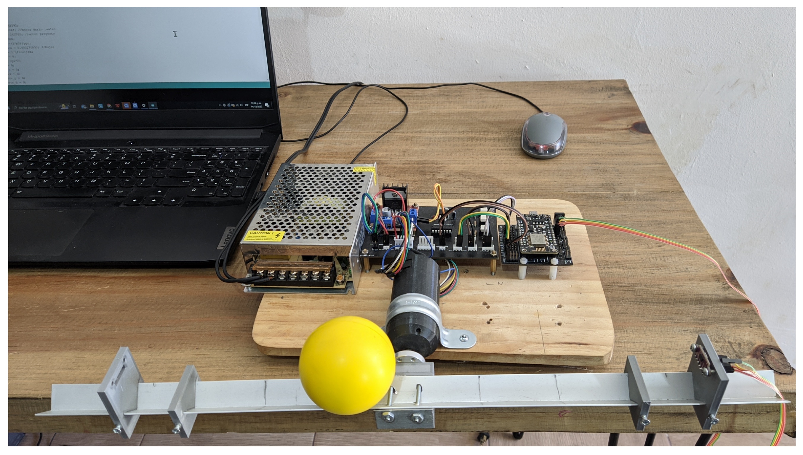
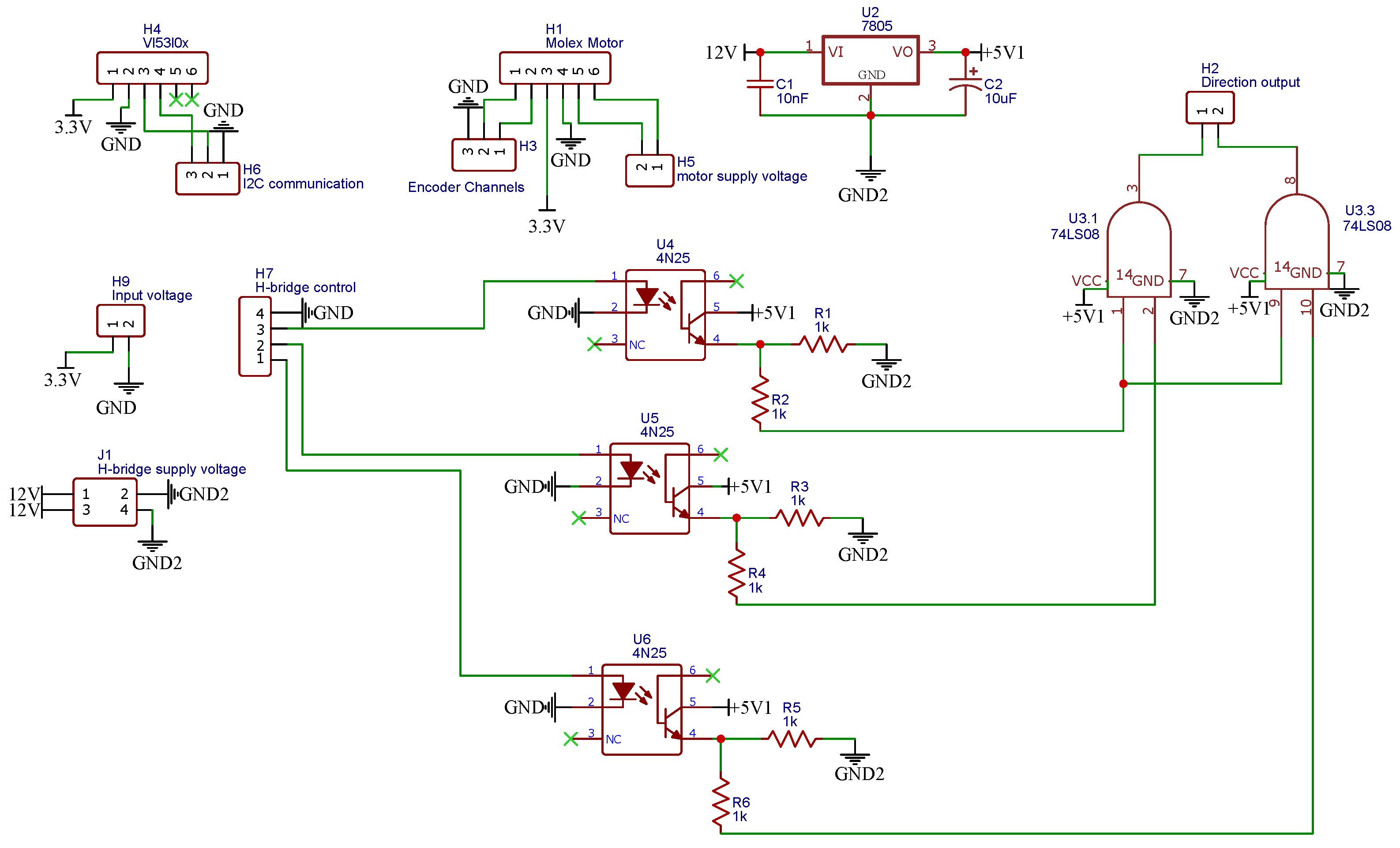
2.1. Description of Platform
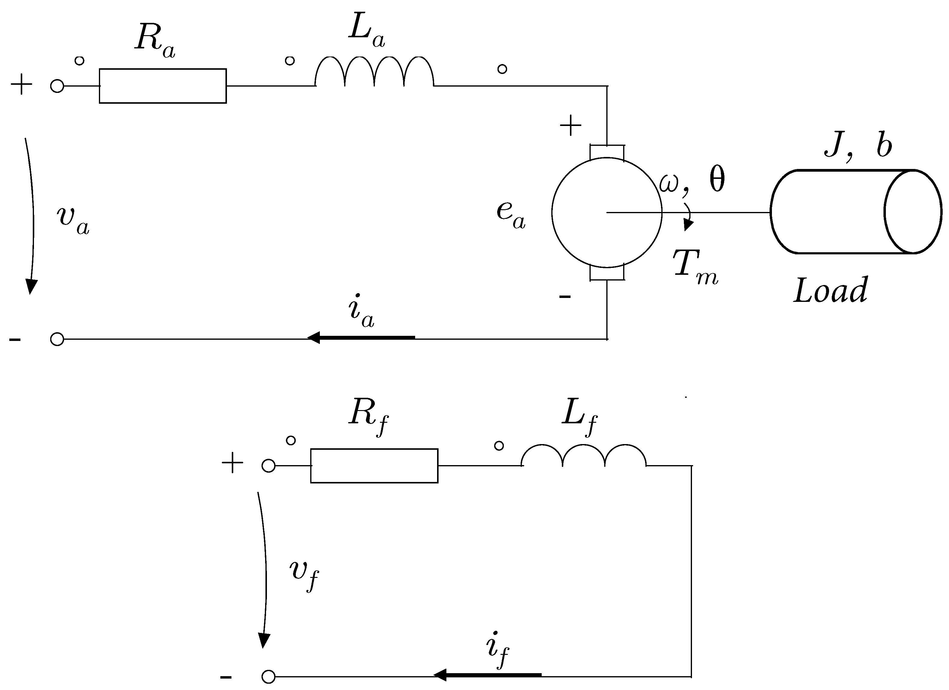
2.2. A Dynamic Model of DC Motor
- The stator provides mechanical support and contains the poles of the machine.
- The rotor, generally cylindrical in shape, is fed with direct current through the collector formed by thin tubes. The blades are usually made of copper and are in alternating contact with the fixed brushes.
Proposal for DC Motor Identification
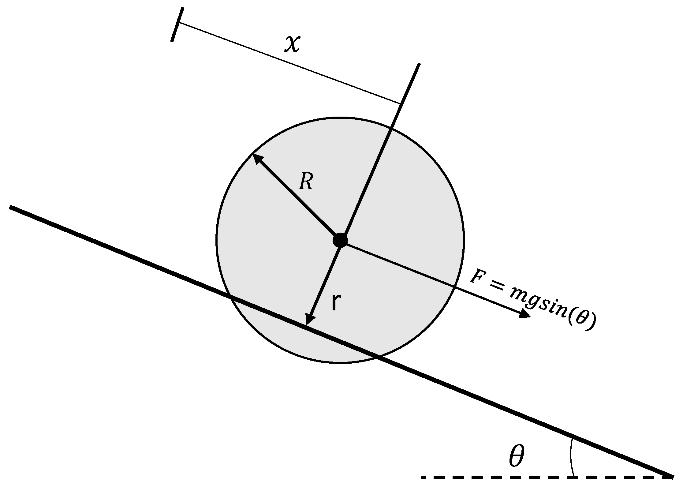
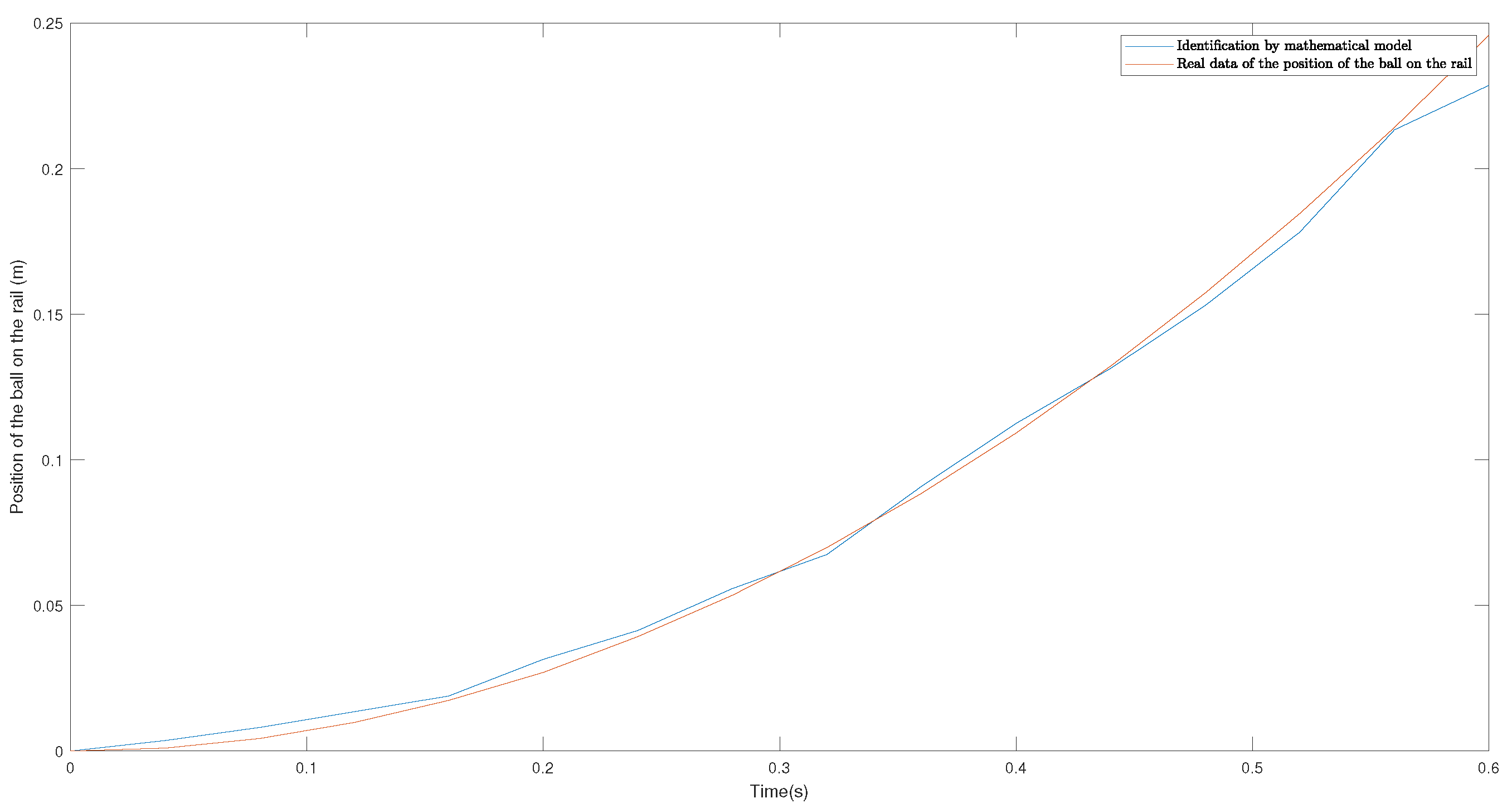
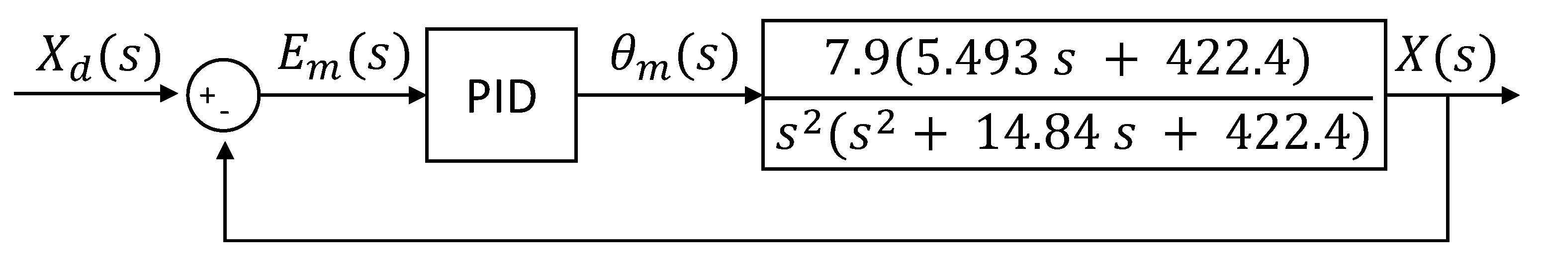
2.3. A Dynamic Model of Ball and Beam
Proposal for Ball and Beam Identification
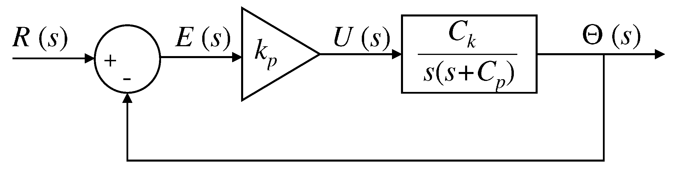
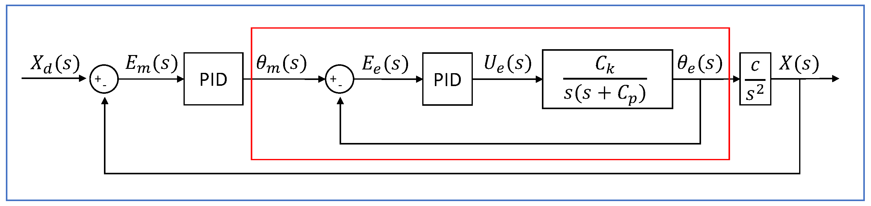
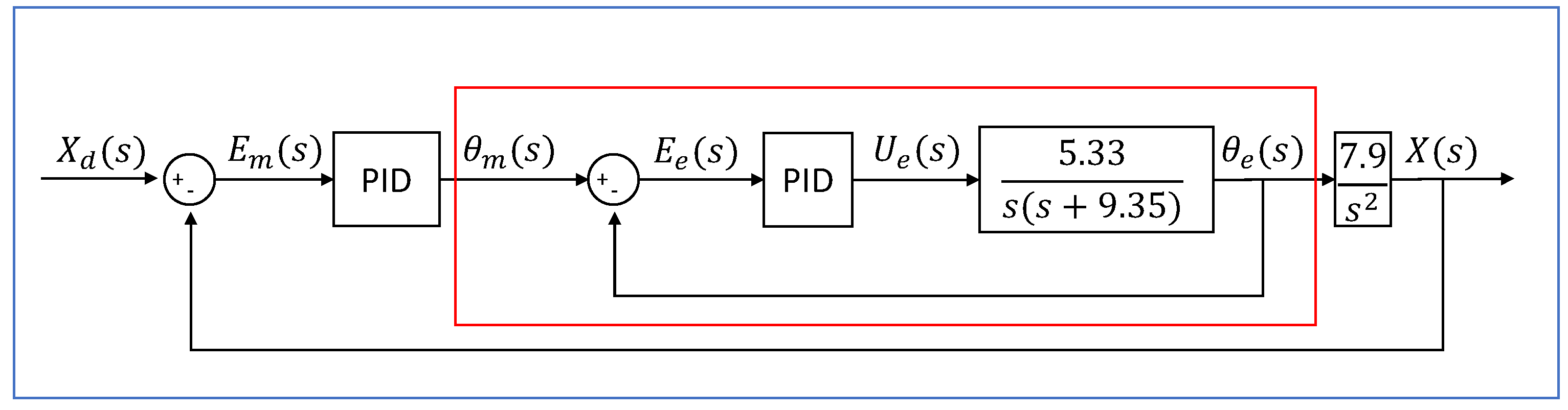
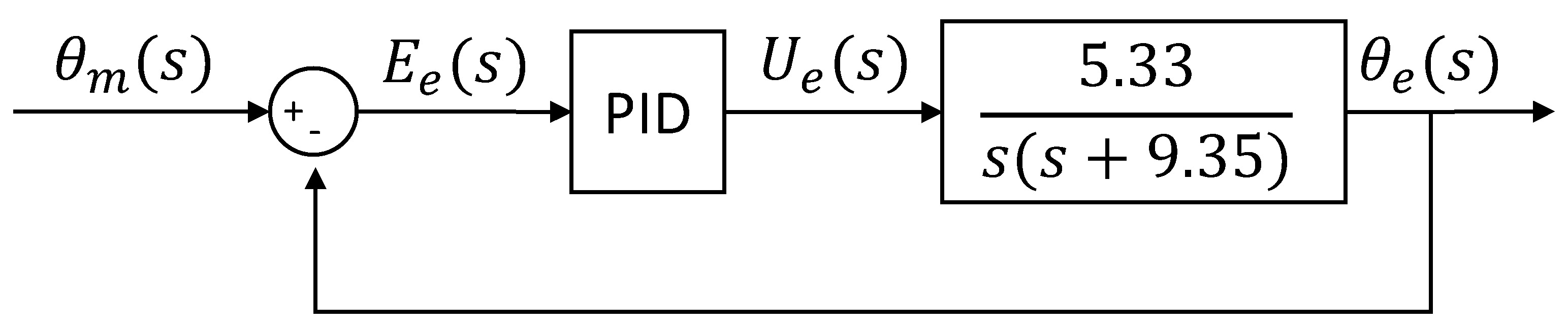
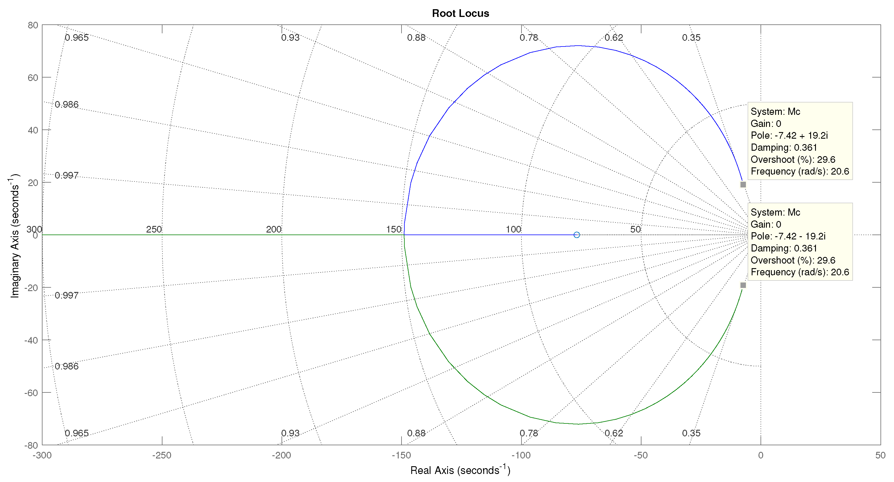
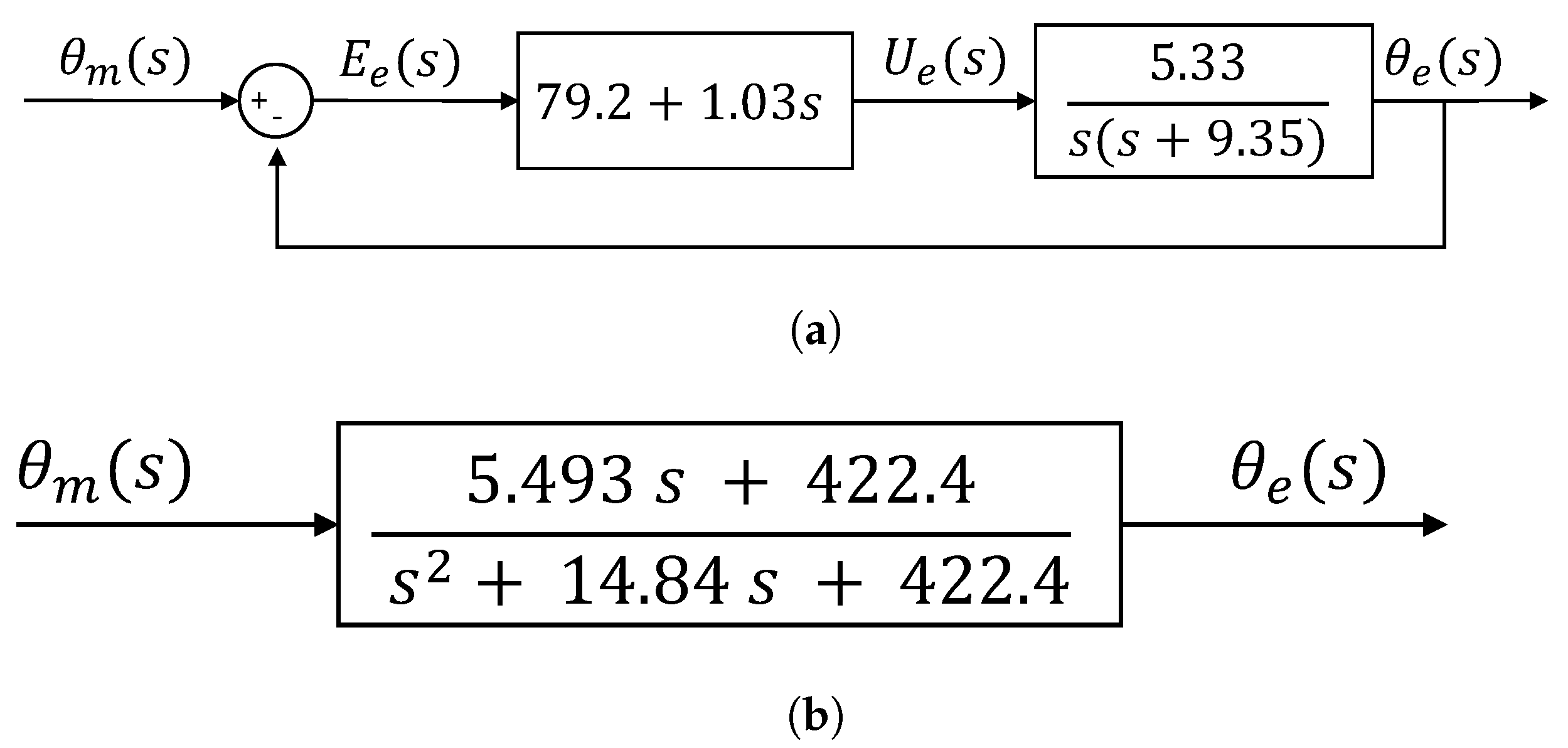
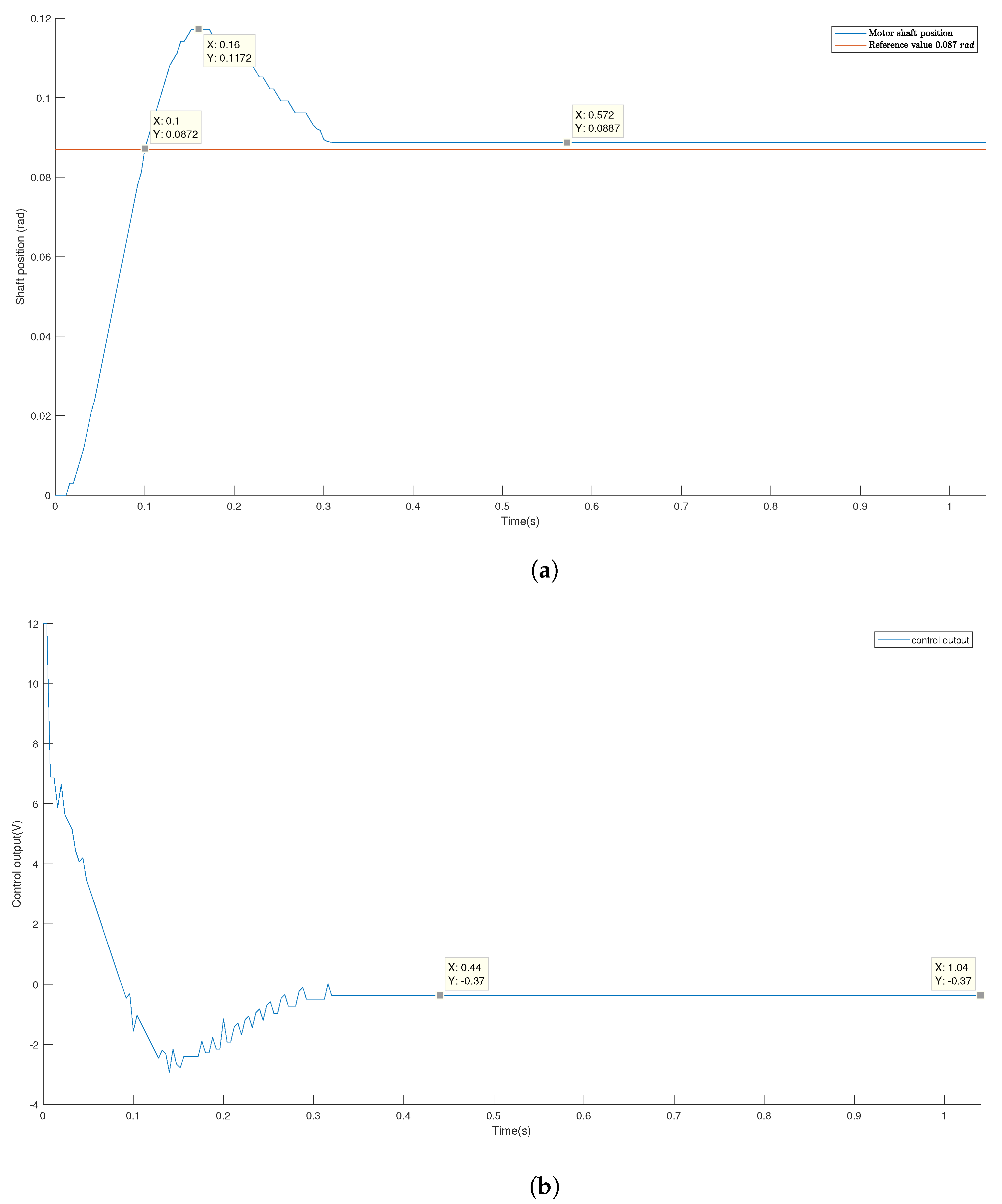
2.4. PID Controller
| Algorithm 1 PID control pseudocode for motor shaft position. |
|
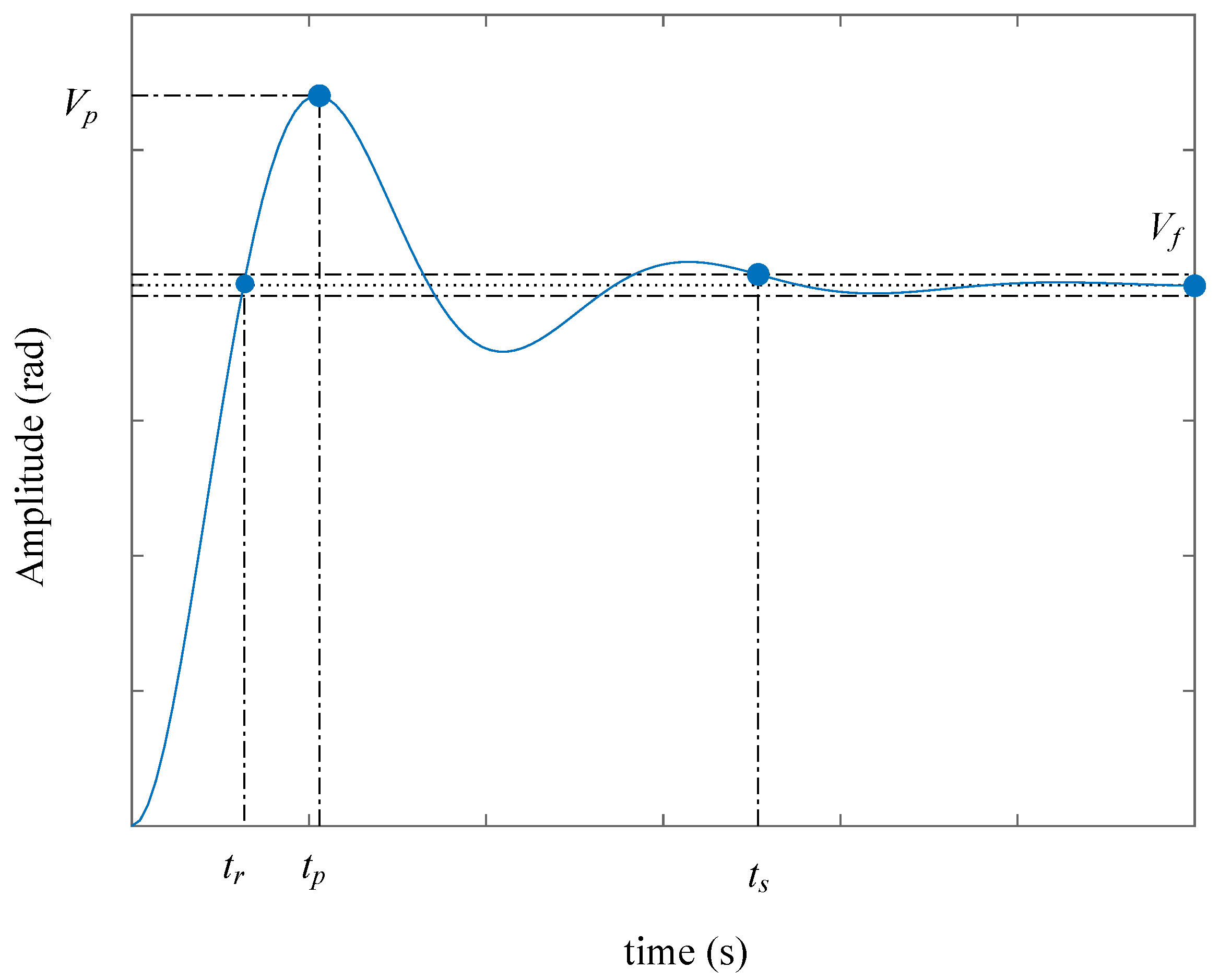
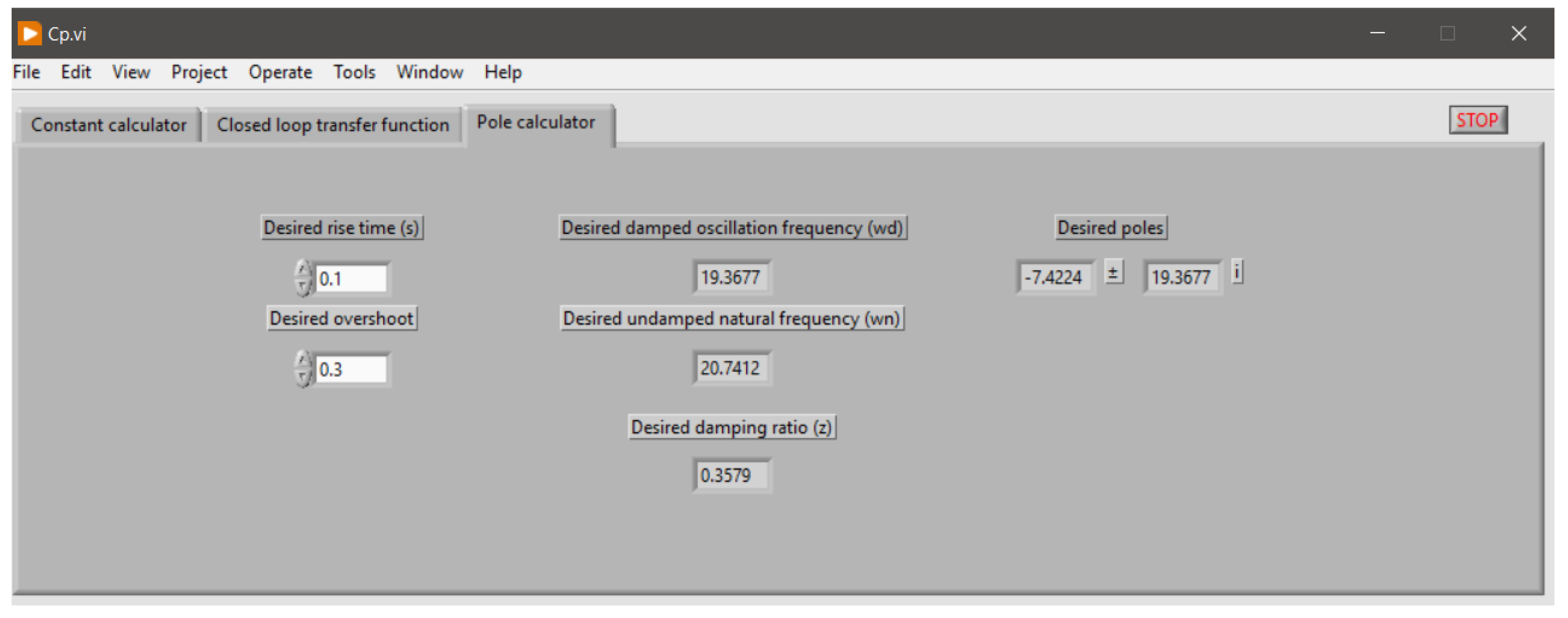
Proposal for PID Controller Tuning
3. Practical Sequence and Project Evaluation
- College-level mathematics: College -level mathematics consist of mathematics that require a degree of mathematical sophistication. Some examples of college-level math include calculus, differential equations, probability, statistics, linear algebra, and discrete math.
- Complex Engineering Problems: Complex engineering problems include one or more of the following characteristics: they involve far-reaching or conflicting technical problems that have no obvious solution; address problems not covered by current standards and codes; involve diverse groups of stakeholders, including many components or sub-issues, involving multiple disciplines or having significant consequences in various contexts.
- Engineering Design: This is creating a system, component, or process to meet desired needs and specifications within constraints. It is an iterative, creative, and decision-making process in which basic science, mathematics, and engineering science are applied to turn resources into solutions.
- Engineering sciences: These build on basic math and science, but take knowledge further into the creative application needed to solve engineering problems. These studies bridge basic mathematics and science on the one hand and engineering practice on the other.
- Teamwork: A team involves more than one person working toward a common goal and should include people from diverse backgrounds, skills, or perspectives.
- The ability to identify, formulate, and solve complex engineering problems by applying engineering, science, and mathematics principles.
- The ability to apply engineering design to produce solutions that meet specific needs considering public health, safety, and welfare, as well as global, cultural, social, environmental, and economic factors.
- Functioning effectively on a team whose members provide leadership, create a collaborative and inclusive environment, set goals, plan tasks, and meet objectives.
- The ability to develop and perform appropriate experimentation, analyze and interpret data, and use engineering judgment to conclusions.
- The ability to acquire and apply new knowledge as needed using appropriate learning strategies.
4. Discussion
5. Conclusions
Author Contributions
Funding
Institutional Review Board Statement
Informed Consent Statement
Data Availability Statement
Conflicts of Interest
References
- Rodriguez-Segura, L.; Zamora-Antuñano, M.A.; Rodriguez-Resendiz, J.; Paredes-García, W.J.; Altamirano-Corro, J.A.; Cruz-Pérez, M.Á. Teaching Challenges in COVID-19 Scenery: Teams Platform-Based Student Satisfaction Approach. Sustainability 2020, 12, 7514. [Google Scholar] [CrossRef]
- Wang, C.; Song, W.; Hu, X.; Yan, S.; Zhang, X.; Wang, X.; Chen, W. Depressive, anxiety, and insomnia symptoms between population in quarantine and general population during the COVID-19 pandemic: A case-controlled study. BMC Psychiatry 2021, 21, 1–9. [Google Scholar] [CrossRef]
- La Comisión Económica para América Latina y el Caribe (CEPAL). La Educación en Tiempos de la Pandemia de COVID-19; UNESCO: Paris, France, 2020. [Google Scholar]
- Goodwin, G.C.; Medioli, A.M.; Sher, W.; Vlacic, L.B.; Welsh, J.S. Emulation-based virtual laboratories: A low-cost alternative to physical experiments in control engineering education. IEEE Trans. Educ. 2011, 54, 48–55. [Google Scholar] [CrossRef]
- Bernstein, D.S. Control experiments and what I learned from them: A personal journey. IEEE Control Syst. 1998, 18, 81–88. [Google Scholar]
- Yao, S.; Liu, X.; Zhang, Y.; Cui, Z. Research on solving nonlinear problem of ball and beam system by introducing detail-reward function. Symmetry 2022, 14, 1883. [Google Scholar] [CrossRef]
- Uyanik, I.; Catalbas, B. A low-cost feedback control systems laboratory setup via Arduino-Simulink interface. Comput. Appl. Eng. Educ. 2018, 26, 718–726. [Google Scholar] [CrossRef]
- Martínez-Prado, M.A.; Rodríguez-Reséndiz, J.; Gómez-Loenzo, R.A.; Camarillo-Gómez, K.A.; Herrera-Ruiz, G. Short informative title: Towards a new tendency in embedded systems in mechatronics for the engineering curricula. Comput. Appl. Eng. Educ. 2019, 27, 603–614. [Google Scholar] [CrossRef]
- Valero, M. Challenges, difficulties and barriers for engineering higher education. J. Technol. Sci. Educ. 2022, 12, 551. [Google Scholar] [CrossRef]
- Mahmoodabadi, M.J.; Shahangian, M.M. A new multi-objective artificial bee colony algorithm for optimal adaptive robust controller design. IETE J. Res. 2022, 68, 1251–1264. [Google Scholar] [CrossRef]
- Ocampo-López, C.; Castrillón-Hernández, F.; Alzate-Gil, H. Implementation of integrative projects as a contribution to the major design experience in Chemical Engineering. Sustainability 2022, 14, 6230. [Google Scholar] [CrossRef]
- Ker, C.C.; Lin, C.E.; Wang, R.T. A ball and beam tracking and balance control using magnetic suspension actuators. Int. J. Control 2007, 80, 695–705. [Google Scholar] [CrossRef]
- De la Torre, L.; Guinaldo, M.; Heradio, R.; Dormido, S. The Ball and Beam System: A Case Study of Virtual and Remote Lab Enhancement With Moodle. IEEE Trans. Indus. Inf. 2015, 11, 934–945. [Google Scholar] [CrossRef]
- Candelas, F.A.; García, G.J.; Puente, S.; Pomares, J.; Jara, C.A.; Pérez, J.; Mira, D.; Torres, F. Experiences on using Arduino for laboratory experiments of Automatic Control and Robotics. IFAC-PapersOnLine 2015, 48, 105–110. [Google Scholar] [CrossRef]
- González-Vargas, A.M.; Serna-Ramirez, J.M.; Fory-Aguirre, C.; Ojeda-Misses, A.; Cardona-Ordoñez, J.M.; Tombé-Andrade, J.; Soria-López, A. A low-cost, free-software platform with hard real-time performance for control engineering education. Comput. Appl. Eng. Educ. 2019, 27, 406–418. [Google Scholar] [CrossRef]
- Muftah, M.N.; Faudzi, A.A.M.; Sahlan, S.; Mohamaddan, S. Intelligent position control for intelligent pneumatic actuator with ball-beam (IPABB) system. Appl. Sci. 2022, 12, 11089. [Google Scholar] [CrossRef]
- Rahmat, M.F.; Wahid, H.; Wahab, N.A. Application of intelligent controller in a ball and beam control system. Int. J. Smart Sens. Intell. Syst. 2010, 3, 45–60. [Google Scholar] [CrossRef]
- Abu Rmilah, M.H.Y.; Hassan, M.A.; Bin Mardi, N.A. A PC-based simulation platform for a quadcopter system with self-tuning fuzzy PID controllers. Comput. Appl. Eng. Educ. 2016, 24, 934–950. [Google Scholar] [CrossRef]
- Cruz-Miguel, E.E.; Rodríguez-Reséndiz, J.; García-Martínez, J.R.; Camarillo-Gómez, K.A.; Pérez-Soto, G.I. Field-programmable gate array-based laboratory oriented to control theory courses. Comput. Appl. Eng. Educ. 2019, 27, 1253–1266. [Google Scholar] [CrossRef]
- Odry, Á.; Fullér, R.; Rudas, I.J.; Odry, P. Fuzzy control of self-balancing robots: A control laboratory project. Comput. Appl. Eng. Educ. 2020, 28, 512–535. [Google Scholar] [CrossRef]
- Jiménez-Ramírez, O.; Cárdenas-Valderrama, J.A.; Ordoñez-Sánchez, A.A.; Quiroz-Juárez, M.A.; Vázquez-Medina, R. Digital proportional-derivative controller implemented in low-resource microcontrollers. Comput. Appl. Eng. Educ. 2020, 28, 1671–1682. [Google Scholar] [CrossRef]
- Gutiérrez, C.A.G.; Reséndiz, J.R.; Santibáñez, J.D.M.; Bobadilla, G.M. A model and simulation of a five-degree-of-freedom robotic arm for mechatronic courses. IEEE Lat. Am. Trans. 2014, 12, 78–86. [Google Scholar] [CrossRef]
- Garduno-Aparicio, M.; Rodriguez-Resendiz, J.; Macias-Bobadilla, G.; Thenozhi, S. A multidisciplinary industrial robot approach for teaching mechatronics-related courses. IEEE Trans. Educ. 2018, 61, 55–62. [Google Scholar] [CrossRef]
- Dizon, J.R.C.; Gache, C.C.L.; Cascolan, H.M.S.; Cancino, L.T.; Advincula, R.C. Post-processing of 3D-printed polymers. Technologies 2021, 9, 61. [Google Scholar] [CrossRef]
- Yang, J.; Wu, H.; Hu, L.; Li, S. Robust predictive speed regulation of converter-driven DC motors via a discrete-time reduced-order GPIO. IEEE Trans. Ind. Electron. 2019, 66, 7893–7903. [Google Scholar] [CrossRef]
- Nise, N. Control Systems Engineering, 6th ed.; John Wiley & Sons, Inc.: Hoboken, NJ, USA, 2011. [Google Scholar]
- Dorf, R.; Bishop, R. Modern Control Systems, 13th ed.; Pearson, Upper Saddle River, NJ, USA, 2016, 13th ed.Pearson: Upper Saddle River, NJ, USA.
- Aguado-Behar, A.; Martínez-Iranzo, M. Identificación y Control Adaptativo, 1st ed.; Prentice-Hall: Madrid, Spain, 2003; p. 280. [Google Scholar]
- Angeles, J. Fundamentals of Robotic Mechanical Systems, 3rd ed.; Springer: New York, NY, USA, 2007; p. 549. [Google Scholar]
- Hernández-Guzmán, V.M.; Silva-Ortigoza, R.; Carrillo-Serrano, R.V. Control Automático: Teoría de Diseño, Construcción de Prototipos, Modelado, Identificación y Pruebas Experimentales, 1st ed.; Colección CIDETEC del Instituto Politécnico Nacional: Distrito Federal, México, 2013. [Google Scholar]
- Mehedi, I.M.; Jeza Aljohani, A.; Mottahir Alam, M.; Mahmoud, M.; Abdulaal, M.J.; Bilal, M.; Alasmary, W. Intelligent dynamic inversion controller design for ball and beam system. Comput. Mater. Contin. 2022, 72, 2341–2355. [Google Scholar] [CrossRef]
- Srivastava, V.; Srivastava, S. Hybrid optimization based PID control of ball and beam system. J. Intell. Fuzzy Syst. 2022, 42, 919–928. [Google Scholar] [CrossRef]
- Peters, A.; Vargas, F.; Garrido, C.; Andrade, C.; Villenas, F. Pl-toon: A low-cost experimental platform for teaching and research on decentralized cooperative control. Sensors 2021, 21, 2072. [Google Scholar] [CrossRef]
- Ogata, K. Ingeniería de Control Moderna; Pearson Educación: London, UK, 2010. [Google Scholar]
- Tang, W.J.; Liu, Z.T.; Wang, Q. DC motor speed control based on system identification and PID auto tuning. In Proceedings of the 2017 36th Chinese Control Conference (CCC), Dalian, China, 26–28 July 2017. [Google Scholar]
- Xie, C.; Zhao, X.; Li, K.; Zou, J.; Guerrero, J.M. A new tuning method of multiresonant current controllers for grid-connected voltage source converters. IEEE J. Emerg. Sel. Top. Power Electron. 2019, 7, 458–466. [Google Scholar] [CrossRef]
- Torres-Salinas, H.; Rodríguez-Reséndiz, J.; Estévez-Bén, A.A.; Cruz Pérez, M.A.; Sevilla-Camacho, P.Y.; Perez-Soto, G.I. A Hands-On Laboratory for Intelligent Control Courses. Appl. Sci. 2020, 10, 9070. [Google Scholar] [CrossRef]


| Item | Vendor | Approximate Cost |
|---|---|---|
| 70:1 Metal gearmotor 37D × 70L mm 12 V 64CPR Encoder | Pololu | USD 51 |
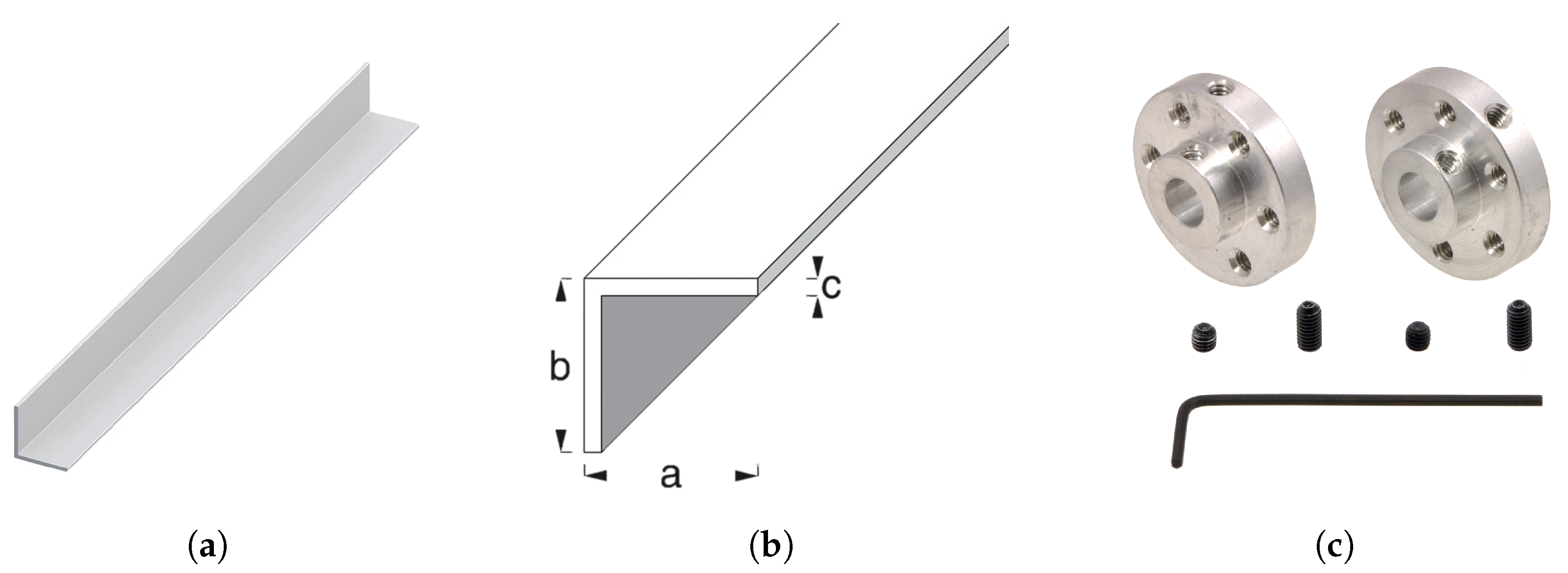
| Universal Aluminum Mounting Hub for 6 mm Shaft | Pololu | USD 9 |
| VL53L0X Time-of-Flight Distance Sensor | Pololu | USD 15 |
| Switching power supply 12 V 10 A | Amazon | USD 24 |
| ESP8266 NODEMCU | Amazon | USD 9 |
| L298N Dual Full-Bridge Motor Driver | Pololu | USD 10 |
| 4n25 Optocoupler (×4) | Newark | USD 3 |
| 74LS08 and gate (×4) | UNIT Electronics | USD 2 |
| Miscellaneous (base, screws, aluminum rail, 3D prints cost) | - | USD 5 |
| GPIO1 | GPIO2 | PWM | Function |
|---|---|---|---|
| DISABLE | DISABLE | DISABLE | Engine braking |
| DISABLE | DISABLE | ENABLE | Engine braking |
| DISABLE | ENABLE | DISABLE | Engine braking |
| DISABLE | ENABLE | ENABLE | Turn left |
| ENABLE | DISABLE | DISABLE | Engine braking |
| ENABLE | DISABLE | ENABLE | Turn right |
| ENABLE | ENABLE | DISABLE | Engine braking |
| ENABLE | ENABLE | ENABLE | Engine braking |
| Relationship | Transfer Function |
|---|---|
| Electromotive force/Armature tension | |
| Armature current/Armature voltage | |
| Angular velocity/Armature tension | |
| Armature position/tension | |
| Motor torque/Armature tension |
| Sensor Values | Position of the Ball on the Rail |
|---|---|
| 329 mm | −0.1 m |
| 267 mm | −0.05 m |
| 217 mm | 0 m |
| 154 mm | 0.05 m |
| 96 mm | 0.1 m |
| 336 mm | −0.1 m |
| 265 mm | −0.05 m |
| 212 mm | 0 m |
| 152 mm | 0.05 m |
| 96 mm | 0.1 m |
| 327 mm | −0.1 m |
| 262 mm | −0.05 m |
| 217 mm | 0 m |
| 158 mm | 0.05 m |
| 94 mm | 0.1 m |
| Practice | Objective | Duration | Expected Results |
|---|---|---|---|
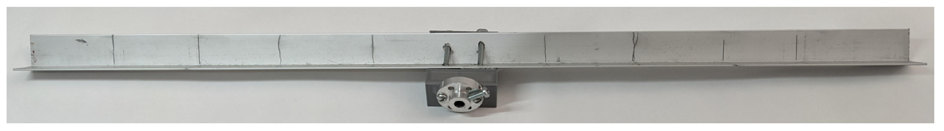
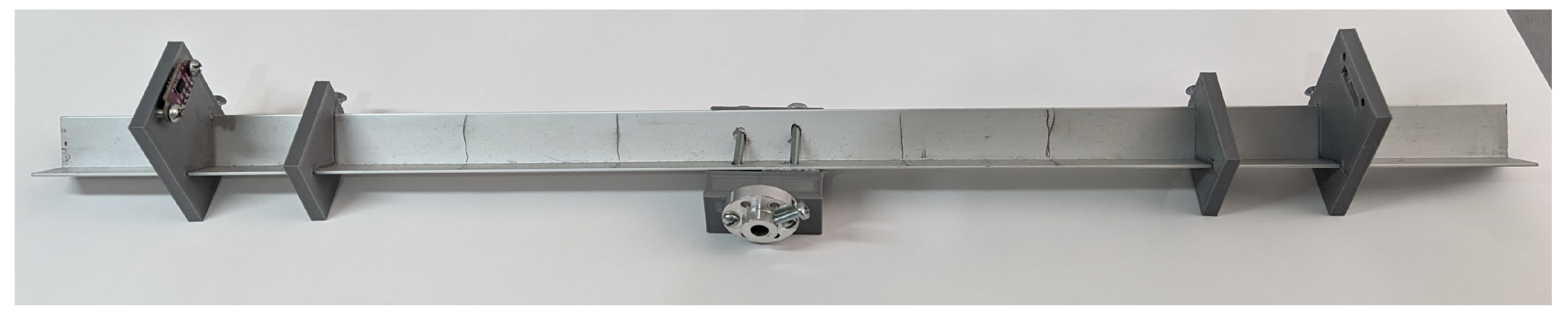
| 1. Hardware description: In this practice, the electronics and hardware are designed and implemented to carry out the ball and beam. | In this practice, the electronics and hardware are designed and implemented to carry out the ball and beam. | 15 h | It is expected that the plant (ball and beam) is in operation, which involves a printed circuit board, the rail, stop pieces, and sensor support. |
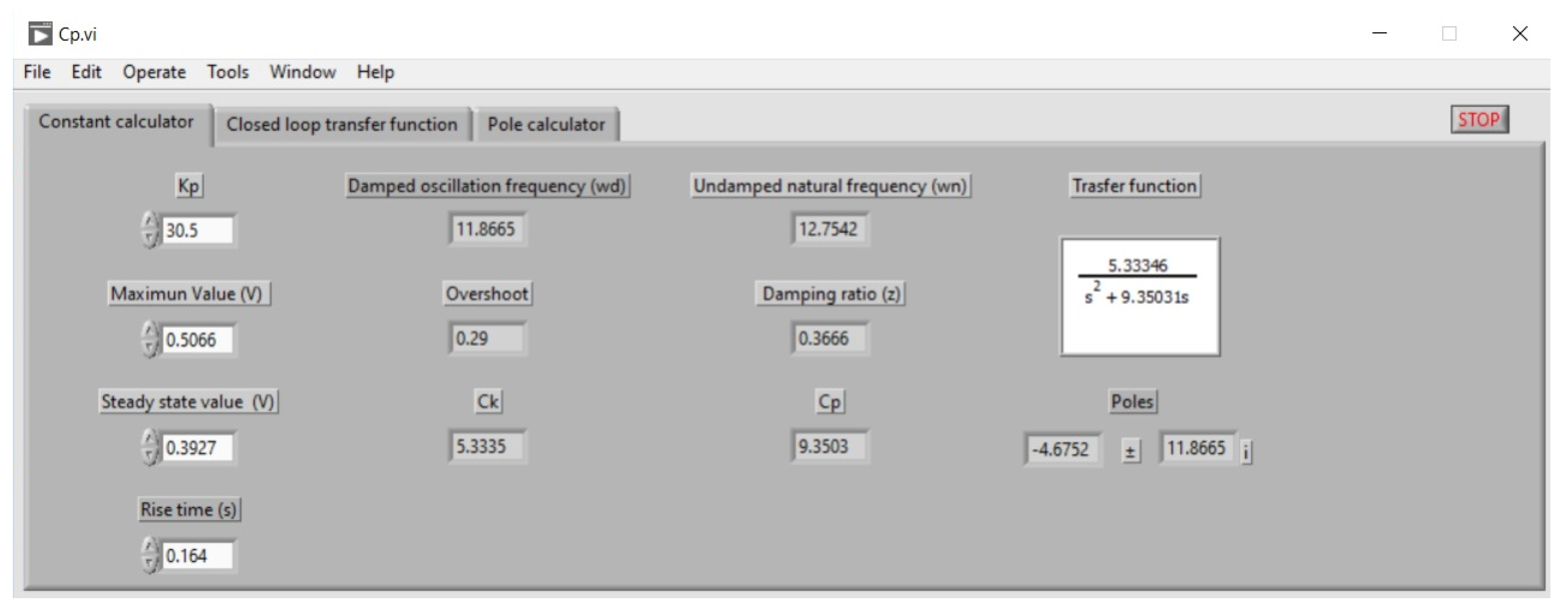
| 2. Graphical user interface: In this practice, the operation of the interface designed for this work is understood, and, in turn, the student is given the necessary tools to develop their own. | The mathematics behind motor model identification is understood. This knowledge is used to develop a user interface focused on DC motor identification based on the interface presented. | 10 h | A user interface is expected to be capable of calculating the constants of the motor transfer function and the poles required to achieve the control instruction. |
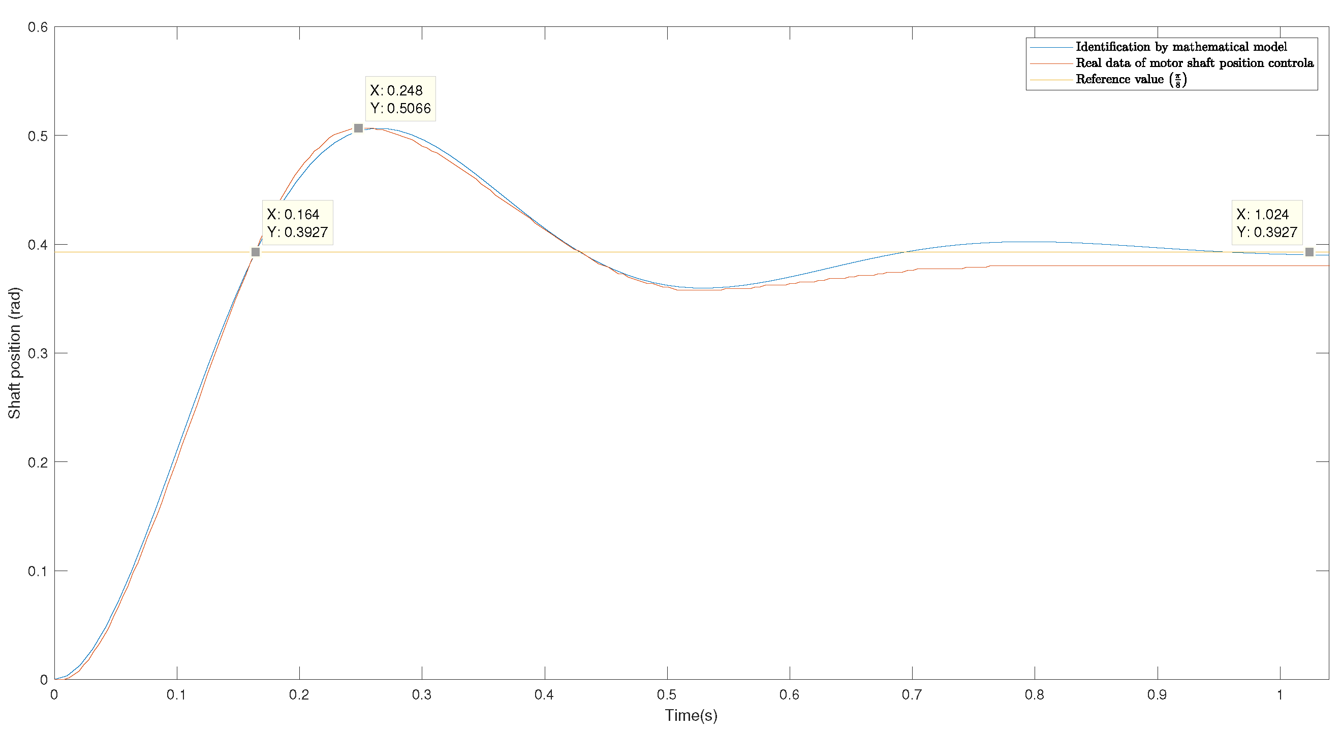
| 3. Identification of DC motor parameters: The motor function was calculated with the interface developed in the previous practice. | That the student can read the data of the encoder to obtain the necessary data for the calculation of the transfer function of the motor. For this objective, it is essential to develop and strengthen knowledge of programming and communication protocols in specific UART. | 10 h | It is expected to have the transfer function that describes the motor and the necessary code for implementing a PID controller. |
| 4. Design and implementation of a PD position controller: Using the locus of the roots, calculate the PID control constants and implement it with the code developed for motor position control in the previous practice. | To understand the importance and effect of each PID constant, in addition to understanding and carrying out the design and implementation of the motor shaft position control, and in addition to facing the non-linearities that real systems present. | 20 h | Position control of the motor shaft that complies with the defined instructions and s. |
| 5. Calibration of the distance sensor and identification of the parameters of the ball on the rail: Once the position control of the motor is obtained, the position sensor is calibrated, taking the center as 0. In addition, the function that models the fall of the ball on the rail is calculated. | In this practice, the objective is to implement the distance sensor, which involves its programming and understanding of the I2C communication protocol, in addition to calculating the c of the transfer function that represents the fall of the ball in order to close the control diagram in the next step. | 5 h | It is expected to have the reading of the position of the ball on the rail in a range of [−0.15 m 0.15 m] in conjunction with the position control of the motor. |
| 6. Design and implementation of a PID distance controller: The PID controller of the master control loop is calculated. Finally, the entire project for controlling the ball on the rail is implemented. | To complete the control loops and carry out the reduction for the calculation of the master PID control. In turn, to develop the software to control the position of the ball on the rail. Finally, to implement it and adjust the calculated control due to non-linearities that were not foreseen in the modeling of the plant. | 25 h | It is expected that, at the end of this practice, the entire plant is operational for the final delivery of the project. |
| Specific Indicators | Criteria | Grade | |||
|---|---|---|---|---|---|
| 90–100 | 70–89 | 60–69 | 0–59 | ||
| The ability to apply the knowledge, techniques, skills, and modern tools that will be applied in engineering and technology activities. The student works in teams | (1) LabVIEW programming (2) Knowledge about digital systems (3) Ability to make measurements with sensors (4) Performs signal conditioning of sensors (5) PCB fabrication according to specific standards (6) Use of communication interfaces (7) Contribute to the team with their theoretical knowledge | Criteria 1 to 6 were almost completed | Criteria 1 to 5 were completed | Criteria 1 to 4 were completed | Criteria 1 to 2 were almost completed |
| The ability to apply knowledge of mathematics, science, engineering, and technology to technological problems that require an application of principles and extensive practical skills | (1) Design and implementation of the controller (2) Application of techniques for tuning the controller (3) Application of mathematical method for identification of parameters of the DC motor (4) Use of auxiliary software for controller design | Criteria 1 to 4 were completed | Criteria 1 to 3 were completed | Criteria 1 to 2 were completed | Criteria 1 was completed |
| The ability to perform tests, standard measurements, and analyze and interpret the experiments | (1) Correct use of units of measurement and scaling (2) Correct use of the sensors (3) Correct interpretation of the output graphs (4) Interpretation of information on applied techniques (root locus) | Criteria 1 to 4 were completed | Criteria 1 to 3 were completed | Criteria 1 to 2 were completed | Criterion 1 was completed |
| The student synthesizes codes with specialized software | (1) Microcontrollers programming (2) Knowledge to design mechanical implementation (3) Implementation of communication protocols (4) Perform a debugging, verification, and optimization of codes using simulation | Criteria 1 to 4 were completed | Criteria 1 to 3 were completed | Criteria 1 to 2 were completed | Criterion 1 was completed |
| The ability to write technical reports and express their ideas, as well as the ability to identify and use technical documentation | (1) Write the laboratory report in detail and in a structured, detailed manner (2) Explain the results and conclusions in detail (3) Include the figures and equations necessary for an appropriate explanation (4) Correctly cites the bibliographical sources (5) Write with appropriate language and correct grammar and spelling | Criteria 1 to 5 were completed | Criteria 1 to 4 were completed | Criteria 1 to 3 were completed | Criteria 1 to 2 were completed |
Disclaimer/Publisher’s Note: The statements, opinions and data contained in all publications are solely those of the individual author(s) and contributor(s) and not of MDPI and/or the editor(s). MDPI and/or the editor(s) disclaim responsibility for any injury to people or property resulting from any ideas, methods, instructions or products referred to in the content. |
© 2023 by the authors. Licensee MDPI, Basel, Switzerland. This article is an open access article distributed under the terms and conditions of the Creative Commons Attribution (CC BY) license (https://creativecommons.org/licenses/by/4.0/).
Share and Cite
Aviles, M.; Rodríguez-Reséndiz, J.; Pérez-Ospina, J.; Lara-Mendoza, O. A Comprehensive Methodology for the Development of an Open Source Experimental Platform for Control Courses. Technologies 2023, 11, 25. https://doi.org/10.3390/technologies11010025
Aviles M, Rodríguez-Reséndiz J, Pérez-Ospina J, Lara-Mendoza O. A Comprehensive Methodology for the Development of an Open Source Experimental Platform for Control Courses. Technologies. 2023; 11(1):25. https://doi.org/10.3390/technologies11010025
Chicago/Turabian StyleAviles, Marcos, Juvenal Rodríguez-Reséndiz, Juan Pérez-Ospina, and Oscar Lara-Mendoza. 2023. "A Comprehensive Methodology for the Development of an Open Source Experimental Platform for Control Courses" Technologies 11, no. 1: 25. https://doi.org/10.3390/technologies11010025