Article

Privacy and Explainability: The Effects of Data Protection on Shapley Values

1
Department of Computing Science, Umeå University, SE-90185 Umeå, Sweden
2
Department of Computer Science, Faculty of Mathematics and Computer, Shahid Bahonar University of Kerman, Kerman 7616913439, Iran
*
Author to whom correspondence should be addressed.
Technologies 2022, 10(6), 125; https://doi.org/10.3390/technologies10060125
Submission received: 25 October 2022 / Revised: 13 November 2022 / Accepted: 21 November 2022 / Published: 1 December 2022
(This article belongs to the Special Issue 10th Anniversary of Technologies—Recent Advances and Perspectives)

Abstract

:
There is an increasing need to provide explainability for machine learning models. There are different alternatives to provide explainability, for example, local and global methods. One of the approaches is based on Shapley values. Privacy is another critical requirement when dealing with sensitive data. Data-driven machine learning models may lead to disclosure. Data privacy provides several methods for ensuring privacy. In this paper, we study how methods for explainability based on Shapley values are affected by privacy methods. We show that some degree of protection still permits to maintain the information of Shapley values for the four machine learning models studied. Experiments seem to indicate that among the four models, Shapley values of linear models are the most affected ones.

1. Introduction

The importance of data privacy has increased in recent years. Data are being gathered and stored in huge quantities and then extensively used for profiling and recommendations. This is a threat for individual privacy. People’s concern has increased in parallel with this increasing storage and use of data. Legislation has been adapted to take into account new threats. European data protection regulation (GDPR) is one of the initiatives to support individual rights. GDPR not only supports data protection and privacy but also requirements on how decision making affecting people should be done. One of them is the requirement that automated decisions should be explainable and that individuals affected by these decisions can request explanations of these decisions.
Data privacy [1,2] provides tools for data anonymization. These tools typically perturb a data set in a way that the modified data do not lead to disclosure. At the same time, perturbation needs to be performed so that the data are still useful [3,4,5]. There are different ways to understand disclosure; this has led to different definitions of privacy. Formal definitions of privacy are known as privacy models. Then, a plethora of data protection mechanisms exists providing solutions according to the different privacy models. These methods can be compared in terms of their privacy guarantees but also with respect to the quality of the resulting data. That is, given a data set and a privacy level, some methods behave better than others for a particular data use. A very simple example is the following: if our goal is to compute a mean of the data set, then microaggregation is better than noise addition. This is so because microaggregation will not change the mean of the data, and noise addition can. For a more complex data analysis, similar studies have been performed. This usually corresponds to study how a data protection mechanism, a masking method or anonymization technique is able to produce a machine learning model of good quality.
The need for explainability [6,7] adds a new element in the machine learning process. A machine learning model needs to be good enough with respect to accuracy or prediction error, in terms of selected performance measures. Nevertheless, this is not enough. We need to provide tools to understand the predictions. Several tools have been developed for this purpose.
To interpret the prediction of machine learning models, there are different methods. They are categorized into main categories. We can distinguish between model-specific and model-agnostic and between global and local methods. For example, global methods focus on the average behavior of the model. They are especially helpful when the user wants to comprehend the general mechanism behind the data. In contrast, models’ individual predictions are explained through local interpretation techniques. In this paper, we focus on explaining individual prediction. For this, we use local models. There are different local model-agnostic methods. They include the Individual Conditional Expectation (ICE), Local Interpretable Model-agnostic Explanations (LIME), counterfactual explanation, Scoped Rules (Anchors), and Shapley values (e.g., SHapley Additive exPlanations). In this work, we use Shapley values [8,9]. Shapley values were introduced by Shapley in 1953 [10] in game theory. We selected this approach because, in the context of explainability, we build a game for a machine learning model that takes into account the interaction of all features. Then, the Shapley value distributes these interactions among the features in a fair way. The theoretical properties of Shapley values have been extensively studied [10,11,12]. So, in short, they provide a summary of interactions between features. In addition, Shapley values have been extensively used in the literature on explainability, and it is easy to compare Shapley values corresponding to different models based on data described in the same features.
Explainability poses a threat to privacy. In short, the more we explain in a model and the less opaque it is, the more information we give in the training data set. Similarly, when data are protected, and models are learned from the data, are explanations still valid? Are the explanations going to change? This is an open problem. Note that there are researchers that state that, from a legal perspective, it is impossible to have both privacy and explainability (see Grant and Wischik [13]). This paper tries to provide some initial results about this research question from a technical perspective. In a previous paper [14], some effects of two anonymization methods (microaggregation and noise addition) on importance features were studied. TreeSHAP [9] was used, which is based on tree-based machine learning models. In this paper, we further study this process with extensive experimentation.
The objective of this paper is to better understand how masking methods affect explanations when these explanations are based on Shapley values. We have conducted extensive experiments with a variety of alternatives. For example, we used three different data sets, four different machine learning algorithms, seven masking strategies, each with a large number of parameters, and different analyses of the results based on the Shapley values. Masking methods include well-established anonymization techniques but also a recently introduced method based on non-negative matrix factorization. The paper does not focus on disclosure risk or utility (from a more classical machine learning perspective). These topics have been studied in several papers, as reported in the literature [1,2,15].
Our results show that
  • Data protection, through masking, does permit explainability using Shapley values, as they are not significantly affected under moderate protection;
  • The use of different machine learning models causes different behaviors in Shapley values. For example, we see that among the methods, linear models are the ones in which Shapley values change the most.
The structure of this paper is as follows. In Section 2, we describe some masking methods we use in this paper. In Section 3, we describe the methodology. In Section 4, we describe the experiments and results. The paper concludes with a summary of our results and some new research directions.

2. Preliminaries

In this section, we review some masking methods for data protection and anonymization and discuss Shapley values as a tool for explainability.

2.1. Masking Methods

Data privacy [1,2,15] provides several methods for data anonymization. They protect a data set by means of modifying it so that sensitive information cannot be disclosed. Masking methods are useful for data publishing, that is, when we need to share data with third parties (e.g., researchers, software engineers, decision makers, etc.) and, particularly, when the data usage is ill-defined or not defined at all. Privacy models for this type of release are k-anonymity [16,17], privacy for re-identification [18,19], and local differential privacy [20,21].
There are three main families of masking methods. Perturbative methods, non-perturbative, and synthetic data generators. Perturbative methods modify the data introducing some kind of error. Noise addition, where a value is replaced by a noisy one, is an example. Rank swapping is another example, in which values are swapped between individuals in order to protect them. In contrast, non-perturbative modifies the data, changing the level of detail but without making it erroneous. For example, replacing a numerical value by an interval, or a town by a county or sets of towns. The interval is more general than the numerical value and, thus, less informative, but there is no error in the information supplied (i.e., the interval). Synthetic data are about replacing the original data by artificial data generated by a model. That is, a machine learning or statistical model is trained with the data, and then the model is used to create artificial data.
In this paper, we used perturbative methods. These methods are preferred to non-perturbative ones because the latter make data processing more complex (e.g., having mixtures of numerical data and intervals, data at different levels of generalization, and sets of values). Synthetic methods are increasingly being used, but we leave them for future work. We discuss below the methods we used in this work.
We use X to denote the original file to be protected, ρ p to denote a masking method with parameter p, and X = ρ p ( X ) , the protected version of X using masking method ρ with parameter p. The following methods are considered in our work.
Microaggregation.
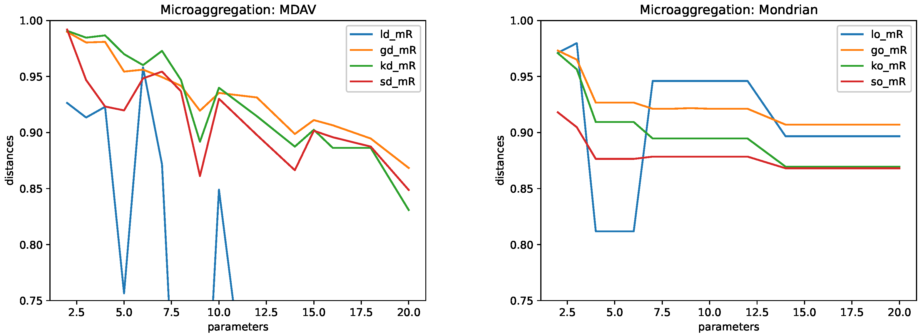
This method consists of building small clusters of the original data and then replacing each original record by the cluster center. Protection is achieved by means of controlling the minimum number of records in a cluster. This corresponds to the parameter k. The larger the k, the larger the protection and the larger the distortion. Microaggregation has been proven to provide a good trade-off between privacy and utility. We used two methods of microaggregation: MDAV [22,23] and Mondrian [24]. That is, two different ways of building the clusters.
Noise addition.
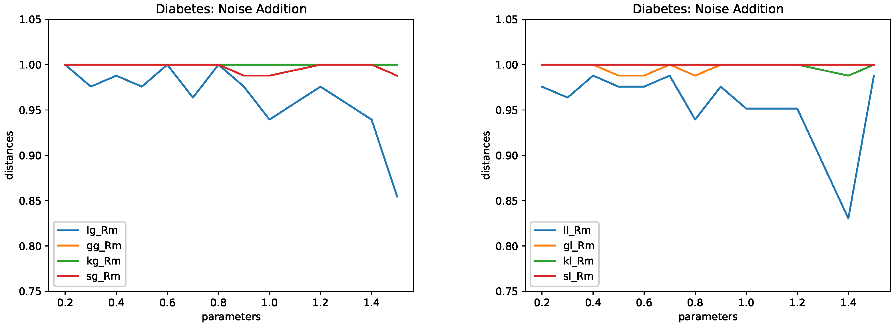
This method replaces each numerical value x by x + ϵ , where ϵ follows a given distribution. We use two types of distributions: a normal distribution with mean zero and standard deviation ( variance * k ) and a Laplace distribution with mean zero and standard deviation as above. Here, k is the parameter. The larger the k, the larger the protection and the larger the distortion.
SVD.
We apply a singular value decomposition to the file, and then rebuild the matrix but only with some of the components. The number of components is a parameter of the system. We use k to denote this parameter. The smaller the number of components, the larger the distortion and larger the privacy.
PCA.
This is similar to the previous method using principal components. We use k to denote the number of components. Therefore, the smaller the k and the number of components, the larger the protection and distortion.
NMF.
This approach corresponds to non-negative matrix factorization [25]. The first use of NMF in data privacy seems to be by Wang et al. [26]. Our approach follows Algorithm 1, and it is based on the implementation of one of the authors [27]. Again, the smaller the number of components k, the larger the privacy. NMF needs the data to be positive, thus, data are scaled into [0,1] before the application of NMF.
Algorithm 1: Algorithm for masking data using NMF. Here, X is the original file with N records and | V | attributes. Protected files X 1 , , X K are produced.
  • Input: X = [ x 1 , , x N ] R | V | × N ; K: maximum rank to consider
  • Output: A = { X k | k 1 , , K } , a family of masked data sets
  • Step 1. For all ranks k 1 , , K
      apply N M F ( X , k ) and find matrices W k and H k
  • Step 2. For all ranks k 1 , , K , do
    • Step 2.1. For each record j = 1 , , N
        construct masked data vectors a j k as follows:
      a j k : = l = 1 k H l j k W l k R | V | ,
    • Step 2.2. Define the masked matrix X k as:
      X k = [ a j k ] j = 1 , , N .
We mentioned above three privacy models related to data sharing. We briefly review these methods and discuss the relationship of the above methods with the privacy models.
Privacy for re-identification is about avoiding identity disclosure. That is, avoiding intruders finding records in the published database. If intruders have information on a particular person (e.g., a record x), then they will try to find x in the protected file X . As data are protected, x will not appear as such in X . So, intruders will try to guess which record x in X corresponds to x. For example, selecting the most similar record x = arg max x X d ( x , x ) . All masking methods are defined to provide privacy for re-identification. Different parameters provide different guarantees. i.e., the larger the distortion, the stronger the guarantee.
Another privacy model is k-anonymity. The goal of this privacy model is to hide a record (or individual) in a set of indistinguishable records (or individuals). A file X satisfies k-anonymity (for a given set of features) when, for each combination of values of the features, we have at least k indistinguishable records. Microaggregation is one of the tools to provide k-anonymity. When we force clusters to have at least k-records, and we replace each record by the cluster centers, we will have that there will be for each combination k indistinguishable records.
Differential privacy is a privacy model focusing on computations. Given a function f and a database X, the goal is to produce a value f ( X ) that does not depend on particular records in X. More formally, a function K f satisfies differential privacy when the result of K f ( X ) is very similar to K f ( X 1 ) , where X and X 1 differ on a single record. The definition presumes that the function K f is a randomized version of f, and then very similar is understood in terms of the similarity between the distribution functions on the space of possible outputs. Local differential privacy is a variation of differential privacy that is appropriate for databases. In this case, individual records are protected independently, with each feature also protected independently. There are different mechanisms to provide differential privacy. The use of Laplacian noise is usual for numerical data. Randomized response (which is equivalent to PRAM) is usual for categorical data. Among the methods discussed above, noise addition with a Laplace distribution is the one that can provide differential privacy. The larger the noise, the larger the privacy guarantees in differential privacy.

2.2. Shapley-Value-Based Explainability

The use of Shapley values as a tool for explainability was introduced by Lundberg and Lee [8]. The motivation is to use game theory machinery [28] as the basis of explanation. A game is a set function defined on a reference set.
In our context, explanations are values for the features expressing their relevance to the outcome of instances (i.e., the columns or attributes of our records). Let us consider some notation. Let x be a record in a data set X and a model M L built from our training data set X. Then, M L ( x ) is the prediction of our model. We consider that X is defined in terms of the features, attributes or variables V.
Then, the game is a set function on sets of features. That is, we consider a subset of features A V and define for x X a function μ x ( A ) . To compute the μ x ( A ) , we consider the output of our model M L if we only knew the attributes in A; for the others, we just have “don’t know”, or e.g., the mean value of the database. Then, μ X ( A ) is the difference between this output and the mean output.
Game theory provides a tool to determine the importance of each feature for a given game. This is known as the Shapley value. In short, given a game μ on the reference set V, its Shapley value is a function that assigns to each feature in V a value in [0,1]. In addition, the addition of all Shapley values is equal to one. These properties hold when the game is positive and normalized. This is not the case here. We may have negative values because μ x ( A ) is a difference that can be negative (the output of a prediction can be smaller than the mean output), and, naturally, is not normalized. Nevertheless, the Shapley values are still useful because they gives a magnitude of the importance of each feature. We have features with positive Shapley values and features with negative Shapley values. The former mean that the feature has a positive influence in the outcome of the model, and the latter represent a negative influence. Then, larger values (in absolute terms) represent larger influence in the outcome. In this way, we know the relevance of features on computing the outcome of a model for a given instance x.

3. Methodology

We implemented the process described in more detail below. It mainly consists of producing different alternative protected files. For a given protected file, we computed a machine learning model, and then for the pair (protected data and machine learning model), we used some records to compute its explanation in terms of the Shapley value. Shapley values obtained through the masked file and through the original file are compared. Different ways of comparison were used. In this way, we can analyze the effects of masking on the Shapley values.
We detail now the methodology for an original data file X. We describe in Section 4 the three actual data sets used in our experiments. The process is described for a particular machine learning algorithm. We use M L : = A ( X ) to denote that M L is the machine learning model trained from data X using algorithm A and use M L ( x ) to denote the outcome of the model when applied to record x (and all features in x are used). We use M L S ( x ) to denote the outcome of the model when applied to record x, and only the features in S are used. The actual 4 machine learning algorithms used in our experiments are also described in Section 4. A summary of the notation used in this section is given in Table 1.
The methodology is described below. We consider different masking methods ρ with parameters p ρ . We use the notation p ρ because parameters depend on the method. When clear, we just use p for the parameters for the sake of conciseness.
  • Split the data set X in training X t r and testing X t e .
  • Define M L o : = A ( X t r ) as the machine learning model learned from the original data.
  • For each x X t e , define its game μ M L o , x according to the existing literature. Formally, for a set of features S, we define μ M L o , x ( S ) = M L o S ( x ) M L o ( x ) . Then, compute the Shapley value ϕ M L o ( x ) of this game. Use all records in X t e to compute the mean Shapley value. We obtain a mean Shapley value for each masking method and parameter. That is, ϕ ¯ M L o , X t e .
  • Produce X ρ p = ρ p ( X t r ) for each pair masking method ρ and parameter p ρ .
  • Produce the corresponding machine learning model M L ρ p : = A ( X ρ p ) .
  • For each x X t e , compute the games and the corresponding Shapley values associated to models M L ρ p . We denote them by μ M L ρ p , x and ϕ M L ρ p ( x ) for each x X t e . Use all records in X t e to compute the mean Shapley value ϕ ¯ M L ρ p , X t e .
  • The following comparisons are considered:
    -
    Compare the mean Shapley of the original and masked files using the Euclidean distance. That is, | | ϕ ¯ M L o , X t e ϕ ¯ M L ρ p , X t e | | .
    -
    Compare the mean Shapley of the original and masked files using Spearman’s rank correlation.
    -
    Compare the Shapley values for each x using the Euclidean distance, and then compute the average distance. Formally, this corresponds to:
    x X t e | | ϕ M L o ( x ) ϕ M L ρ p ( x ) | | | X t e |
    -
    Compare the Shapley values for each x using Spearman’s rank coefficient.
We considered four different comparisons, because we consider that they provide different types of information. The use of mean Shapley values gives information on a global level. Mean Shapley values permit us to know which are the most relevant features in general terms. So, we can observe if these important features are changed because of data protection. Nevertheless, important features in general terms do not need to coincide with the relevant features for a particular example. When the machine learning models are non-linear, this is not necessarily the case. That is why it is also relevant to see if masking data causes changes at the local level. This can be observed with a direct comparison of the Shapley values for x X t e and then averaging these comparisons.
We used the Euclidean distance to compare the Shapley values but also the Spearman rank coefficient. The Shapley values are numerical values, but from the point of view of relevant attributes, the relative order is what matters. We used the Spearman rank coefficient because it only takes into account the relative position and not the values themselves.

4. Experiments and Analysis

In this section, we detail the experiments we have conducted and discuss the results.

4.1. Implementation

Our experiments were conducted in Python. We have our own implementation of the masking methods. We used the sklearn package for machine learning. That is, to find machine learning models from training data. We have our own implementation for computing games and for computing the Shapley value of these games. The Spearman rank correlation coefficient is from the scipy package. Code is available here: [29].

4.2. Parameters

We considered the following parameters for the masking methods described above. In practice, parameter selection depends on the privacy requirements and data utility requirements. For microaggregation, a value of k around 5 is used. Noise addition requires values that depend on the available data and their sensitivity (when implementing differential privacy). PCA and SVD parameters close to the number of features may imply low levels of privacy.
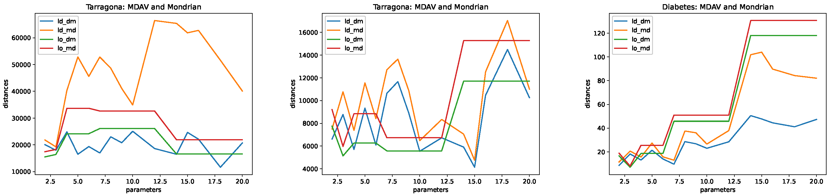
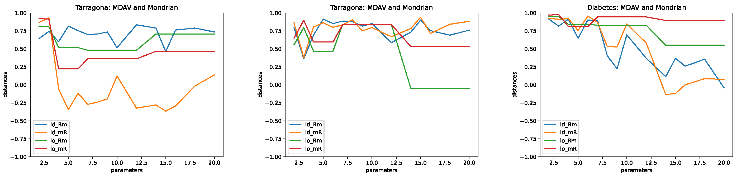
  • Microaggregation. As explained above, we considered two different microaggregation algorithms: MDAV and Mondrian. The difference in the algorithms is in how clusters are built. For both algorithms, the cluster centers are defined in terms of the means of the associated records. The following values of the parameter k were used: k = { 2 , 3 , 4 , 5 , 6 , 7 , 8 , 9 , 10 , 12 , 14 , 15 , 16 , 18 , 20 } .
  • Noise addition. We considered Normal and Laplacian distribution. The following values of k were used: k = { 0.2 , 0.3 , 0.4 , 0.5 , 0.6 , 0.7 , 0.8 , 0.9 , 1.0 , 1.2 , 1.4 , 1.5 } .
  • SVD. We considered the singular value decomposition and the reconstruction of the matrix using different number of values. In our experiments, we considered k = { 2 , 3 , 4 , 5 , 6 , 7 , 8 } .
  • PCA. As in the case of SVD, we considered k = { 2 , 3 , 4 , 5 , 6 , 7 , 8 } .
  • NMF. The selection of the parameter that approximates well the matrix is a difficult problem [30]. We considered here a different number of components in the factorization. We used k = { 2 , 3 , 4 , 5 , 6 , 7 , 8 } .

4.3. Data Sets and Machine Learning Algorithms

We applied our method to the following data sets. They were selected because they are well-known in the literature and used before in both machine learning as well as data privacy [31] research. Only numerical data were considered. Data are available in the UCI repository [32] and in the sklearn Python library. We leave non-numerical data for future work.
  • Tarragona. This data set contains 834 records described in terms of 13 attributes. We used the first 12 attributes as the independent ones and the 13th attribute (last column in the file) as the dependent one.
  • Diabetes. This data set contains 442 records with information on 10 attributes. An additional numerical attribute is also included in the data set, for prediction.
  • Iris. This data set contains 150 records described in terms of 4 attributes and a class (which corresponds to a fifth attribute). We used the 4 attributes as the independent variables, used the class as a numerical value, and used one as a numerical dependent.

4.4. Machine Learning Algorithms

We considered different machine learning algorithms, supplied by sklearn. In particular, we considered the methods (used in all cases with default parameters)
  • linear_model.LinearRegression (linear regression);
  • sklearn.linear_model.SGDRegressor (linear model implemented with stochastic gradient descent);
  • sklearn.kernel_ridge.KernelRidge (linear least squares with l2-norm regularization, with the kernel trick);
  • sklearn.svm.SVR (Epsilon-Support Vector Regression).
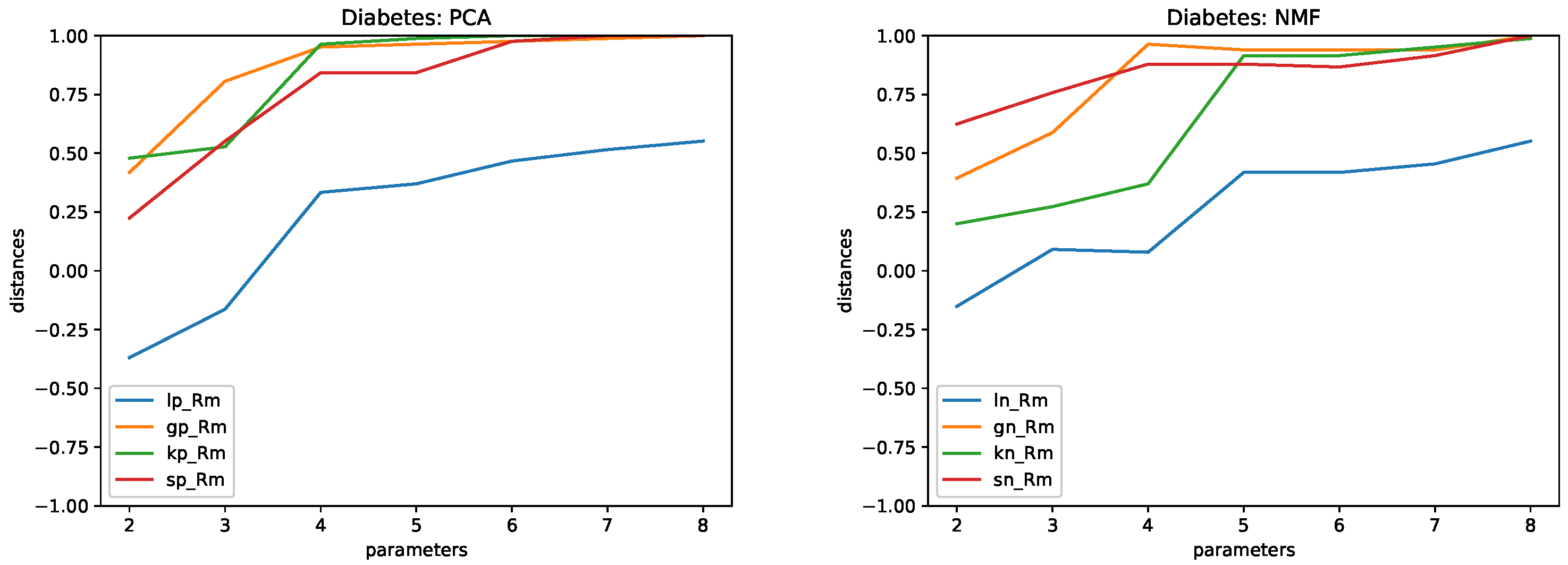
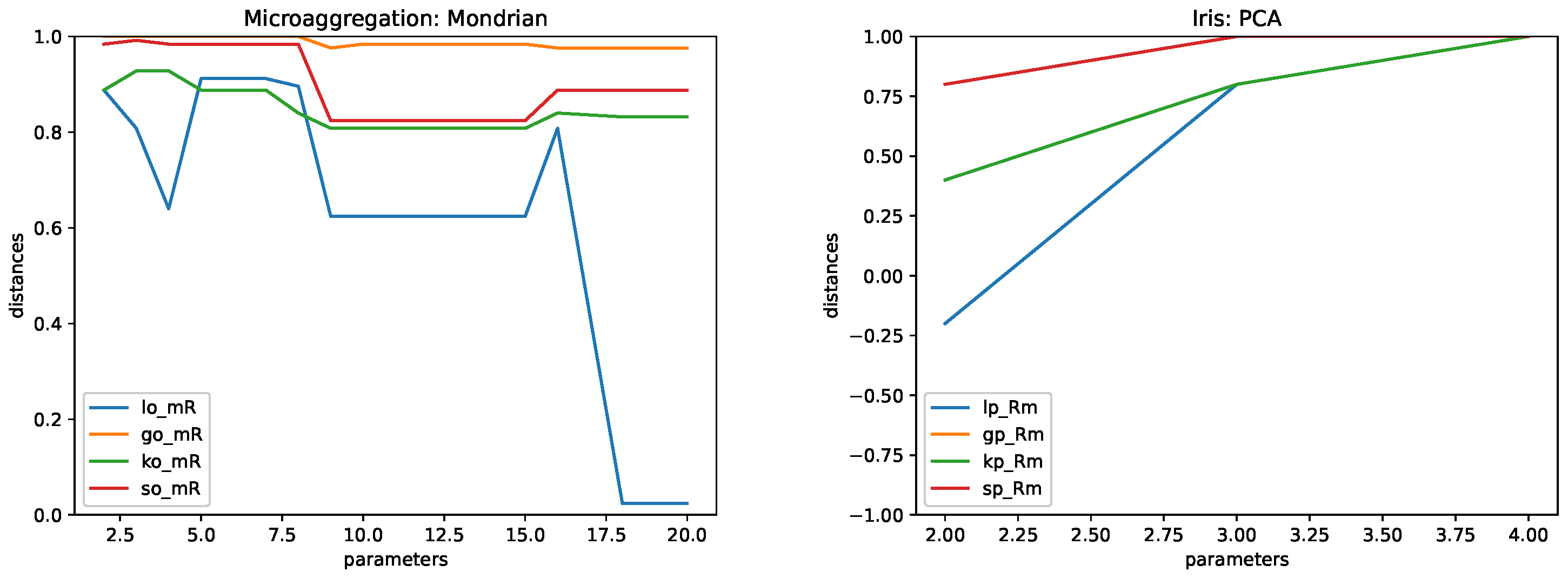
These algorithms were applied using dependent and independent attributes, as described in the previous section. The standard versions of these algorithms were used.

4.5. Results

An analysis of the results leads to the following conclusions.
The first observation is that both the mean distance between Shapley values and the distance between Shapley values can be very large. Note that when the game is defined for a particular machine learning algorithm, the game is unbounded and depends on the values of the prediction. That is, the value of the game for a set may be very large if the prediction is large. Because of this, the Shapley values can be large and, thus, the distance between two Shapley values can also be large. This makes comparisons cumbersome. This is illustrated in Figure 1, which shows (left) the distances for the Tarragona data set and (right) the distances for the Diabetes data set. It is not so easy to compare the scales of the two figures. Moreover, considering 11 or 12 independent inputs (left and middle figures) changes the scale. In contrast, the rank correlation is always in the [−1,1] interval, which makes comparisons easier. This is illustrated in Figure 2.
These figures also show that larger distances do not mean larger rank correlation. That is, the the distances between Shapley values do not mean that the order of these values are changed so much. Observe that, for the set Diabetes, in Figure 1, Mondrian give larger distances than MDAV (i.e., curves lo_dm and lo_md have larger values than curves ld_dm and ld_md). That is, MDAV seems to behave better with larger amounts of noise. In contrast, in Figure 2, it is MDAV which shows a worse performance, as Mondrian has a rank correlation near to 1 for larger parameters. The set Tarragona seems to have a more erratic behavior on the distances and rank correlations with respect to the parameters but is more consistent if we compare Figure 1 and Figure 2. It can also be seen that when considering more input attributes, the curves seem to have a better shape. Compare left and middle curves in these figures, where the distances are smaller and correlations are larger.
Now, we show that we obtain similar changes on the rank correlation independently of the machine learning method used. Figure 3 includes the results for MDAV (left) and Mondrian (right). We compare the mean rank correlation of all Shapley values computed using the four different machine learning algorithms considered in the paper. We can see that the results are quite similar, except for the case of linear regression and MDAV. The scale of the figure was set to [0.75,1] to better visualize the results.
This similar behavior appears also with other masking methods. In Figure 4, we have the case of noise addition, with both types of noise (Gaussian noise and Laplacian noise). It is interesting to underline that the linear model is the one that has a larger effect on the rank correlation, and as it can be seen in the figure for microaggregation, it also happens in MDAV. In fact, the same behavior is also reproduced for protection with SVD, PCA, and NMF. Figure 5 includes the curves for PCA and NMF. The one for SVD is not included, but the resulting figure is almost the same as the one for PCA. It is relevant to underline that the parameters of SVD, PCA, and NMF are a kind of reversal to the ones of microaggregation and noise. That is, the smaller the parameter k, the larger the protection. That is why the curves in Figure 5 are increasing instead of decreasing.
The figures discussed so far correspond to the Tarragona and Diabetes files. The results for the Iris data set are consistent with the findings of these two files, although the curves have additional noise. We consider that this is due to the fact that the data file is smaller, and the effects of the same amount of masking on the machine learning models are larger. This affects the rank correlation of the Shapley value of the variables. Compare Figure 6 with the results of masking with Mondrian and PCA for the Iris data set and Figure 3 (left, Mondrian for Diabetes) and Figure 5 (right, PCA for Diabetes).

5. Conclusions

There is an increasing need for explainability in the context of machine learning models and automated decisions. Nevertheless, machine learning models and automated decisions need to be compliant with privacy requirements. At present, there is no clear understanding of how explainability and privacy are incompatible, or if some levels of explainability are possible when privacy guarantees are ensured. There are claims [13] that having both is impossible. This work studied this problem in a particular scenario.
More particularly, we studied the effect of machine learning algorithms on explainability, when the latter are implemented in terms of the Shapley value. That is, we studied how masking affects Shapley values. Different analyses were performed: one based on differences in the Shapley values and another based on rank correlation of these Shapley values.
These results seem to indicate that protection does not prevent explainability when this is implemented using Shapley values. That is, that under some assumptions, explainability and privacy are not incompatible. We saw that the results based on rank correlation have a sounder behavior (they change more smoothly with respect to protection) and have a similar behavior for different machine learning models than the results based on the difference of the values (difference computed in terms of the norm). In this case, the fact that rank correlation is better than the norm means that what seems to be relevant is the order of the variables with respect to the Shapley values and not the values themselves.
The analysis has also shown that among the four machine learning models, the linear model is the one that has the worst performance with respect to the Shapley value. That is, the relevance of the features changes the most. This seems to be a constant independent of the masking method applied to the data.
It is important to note that tools for explainability [6,7] are to be used by humans when decisions are being automated. Then, the study of explainability is incomplete without the user perspective. This also applies here. We considered and compared the results of the Shapley values, but we did not perform any user study on what users can consider relevant in this setting. In our analysis, we considered all Shapley values; future work may consider the most significant Shapley values. Note that in our context, the most significant seem to be the larger ones in absolute value, as the game can take negative values.
In this study, we focused on numerical data files of a relatively small size. The computational requirements of the analysis become challenging for larger files. The results seem to indicate that the larger the file, the more robust the results of Shapley. We plan to study if this is the case. In addition, we plan to further analyze local effects. We considered Shapley because it is good as a way to evaluate local explainability. For large data sets, it is difficult to analyze and compare these local results. We need to study these local effects in large data sets along with other criteria.
In this paper, we studied the effects of masking into explainability when the latter is expressed in terms of Shapley values. We showed that explainability is not incompatible with privacy for this limited scenario. We plan to extend this work considering other tools related to explainability as, for example, logic-based explanations.

Author Contributions

Conceptualization, A.B. and V.T.; software, V.T. (NMF-based masking by L.A.); validation, A.B. and L.A.; writing—original draft preparation, V.T., with contributions by A.B. and L.A.; writing—review and editing, A.B., L.A. and V.T.; funding acquisition, V.T. All authors have read and agreed to the published version of the manuscript.

Funding

This study was partially funded by the Wallenberg AI, Autonomous Systems and Software Program (WASP) funded by the Knut and Alice Wallenberg Foundation.

Institutional Review Board Statement

Not applicable.

Informed Consent Statement

Not applicable.

Data Availability Statement

We used publicly available data. References were supplied.

Conflicts of Interest

The authors declare no conflict of interest.

References

  1. Hundepool, A.; Domingo-Ferrer, J.; Franconi, L.; Giessing, S.; Nordholt, E.S.; Spicer, K.; de Wolf, P.-P. Statistical Disclosure Control; Wiley: Hoboken, NJ, USA, 2012. [Google Scholar]
  2. Torra, V. Data Privacy: Foundations, New Developments and the Big Data Challenge; Springer: Berlin/Heidelberg, Germany, 2017. [Google Scholar]
  3. Abowd, J.; Ashmead, R.; Cumings-Menon, R.; Garfinkel, S.; Kifer, D.; Leclerc, P.; Sexton, W.; Simpson, A.; Task, C.; Zhuravlev, P. An Uncertainty Principle Is a Price of Privacy-Preserving Microdata. In Proceedings of the 35th Conference on Neural Information Processing Systems, Virtual, 6–14 December 2021. [Google Scholar]
  4. Pastore, A.; Gastpar, M.C. Locally differentially-private randomized response for discrete distribution learning. J. Mach. Learn. Res. 2021, 22, 1–56. [Google Scholar]
  5. Reimherr, M.; Awan, J. Elliptical Perturbations for Differential Privacy. In Proceedings of the NeurIPS 2019, Vancouver, BC, Canada, 8–14 December 2019. [Google Scholar]
  6. Riveiro, M.; Thill, S. The challenges of providing explanations of AI systems when they do not behave like users expect. In Proceedings of the 30th ACM Conference on User Modeling, Adaptation and Personalization, Barcelona, Spain, 4–7 July 2022; pp. 110–120. [Google Scholar]
  7. Riveiro, M.; Thill, S. “That’s (not) the output I expected!” On the role of end user expectations in creating explanations of AI systems. Artif. Intell. 2021, 298, 103507. [Google Scholar] [CrossRef]
  8. Lundberg, S.M.; Lee, S.I. A unified approach to interpreting model predictions. In Proceedings of the NeurIPS 30, Long Beach, CA, USA, 4–9 December 2017. [Google Scholar]
  9. Lundberg, S.M.; Erion, G.; Chen, H.; DeGrave, A.; Prutkin, O.M.; Nair, B.; Katz, R.; Himmelfarb, J.; Bansal, N.; Lee, S.-I. Explainable AI for Trees: From Local Explanations to Global Understanding. arXiv 2019, arXiv:1905.04610. [Google Scholar] [CrossRef] [PubMed]
  10. Shapley, L. A value for n-person games. Ann. Math. Stud. 1953, 28, 307–317. [Google Scholar]
  11. Dubey, P. On the uniqueness of the Shapley value. Int. J. Game Theory 1975, 4, 131–140. [Google Scholar] [CrossRef]
  12. Roth, A.E. (Ed.) The Shapley Value; Cambridge University Press: Cambridge, MA, USA, 1988. [Google Scholar]
  13. Grant, T.D.; Wischik, D.J. Show Us the Data: Privacy, Explainability, and Why the Law Can’t Have Both. Geo. Wash. L. Rev. 2020, 88, 1350. [Google Scholar]
  14. Bozorgpanah, A.; Torra, V. Explainable machine learning models with privacy. 2021; manuscript. [Google Scholar]
  15. Torra, V. A Guide to Data Privacy; Springer: Berlin/Heidelberg, Germany, 2022. [Google Scholar]
  16. Samarati, P. Protecting Respondents’ Identities in Microdata Release. IEEE Trans. Knowl. Data Eng. 2001, 13, 1010–1027. [Google Scholar] [CrossRef] [Green Version]
  17. Samarati, P.; Sweeney, L. Protecting Privacy When Disclosing Information: k-Anonymity and Its Enforcement through Generalization and Suppression; SRI International Technical Report, 1998. Available online: https://epic.org/wp-content/uploads/privacy/reidentification/Samarati_Sweeney_paper.pdf (accessed on 23 September 2022).
  18. Jaro, M.A. Advances in record-linkage methodology as applied to matching the 1985 Census of Tampa, Florida. J. Am. Stat. Assoc. 1989, 84, 414–420. [Google Scholar] [CrossRef]
  19. Winkler, W.E. Re-identification methods for masked microdata, PSD 2004. Lect. Notes Comput. Sci. 2004, 3050, 216–230. [Google Scholar]
  20. Evfimievski, A.; Gehrke, J.; Srikant, R. Limiting privacy breaches in privacy preserving data mining. In Proceedings of the Twenty-Second ACM SIGMOD-SIGACT-SIGART Symposium on Principles of Database Systems, San Diego, CA, USA, 9–12 June 2003. [Google Scholar]
  21. Kasiviswanathan, S.P.; Lee, H.K.; Nissim, K.; Raskhodnikova, S.; Smith, A. What can we learn privately? In Proceedings of the Annual Symposium on Foundations of Computer Science, Washington, DC, USA, 25–28 October 2008. [Google Scholar]
  22. Domingo-Ferrer, J.; Mateo-Sanz, J.M. Practical data-oriented microaggregation for statistical disclosure control. IEEE Trans. Knowl. Data Eng. 2002, 14, 189–201. [Google Scholar] [CrossRef] [PubMed] [Green Version]
  23. Domingo-Ferrer, J.; Martinez-Balleste, A.; Mateo-Sanz, J.M.; Sebe, F. Efficient Multivariate Data-Oriented Microaggregation. Int. J. Very Large Databases 2006, 15, 355–369. [Google Scholar] [CrossRef]
  24. LeFevre, K.; DeWitt, D.J.; Ramakrishnan, R. Multidimensional k-Anonymity; Technical Report 1521; University of Wisconsin: Madison, WI, USA, 2005. [Google Scholar]
  25. Lee, D.D.; Seung, H.S. Learning the parts of objects by non-negative matrix factorization. Nat. Vol. 1999, 401, 788–791. [Google Scholar] [CrossRef] [PubMed]
  26. Wang, J.; Zhang, J. NNMF-based factorization techniques for high-accuracy privacy protection on non-negative-valued datasets. In Proceedings of the Sixth IEEE International Conference on Data Mining—Workshops (ICDMW’06), Hong Kong, China, 18–22 December 2006. [Google Scholar]
  27. Aliahmadipour, L.; Valipour, E. A new method for preserving data privacy based on the non-negative matrix factorization clustering. Fuzzy Syst. Its Appl. 2022. (In Persian) [Google Scholar] [CrossRef]
  28. Myerson, R.B. Game Theory; Harvard University Press: Cambridge, MA, USA, 1991. [Google Scholar]
  29. Code Python of Our Software. Available online: www.mdai.cat/code (accessed on 23 September 2022).
  30. Berry, M.W.; Browne, M.; Langville, A.M.; Pauca, V.P.; Plemmons, R.J. Algorithms and applications for approximate nonnegative matrix factorization. Comput. Stat. Data Anal. 2007, 52, 155–173. [Google Scholar] [CrossRef]
  31. Brand, R.; Domingo-Ferrer, J.; Mateo-Sanz, J.M. Reference Datasets to Test and Compare SDC Methods for Protection of Numerical Microdata; Technical Report; European Project IST-2000-25069 CASC, 2002; Available online: https://research.cbs.nl/casc/CASCrefmicrodata.pdf (accessed on 23 September 2022).
  32. Dua, D.; Graff, C. UCI Machine Learning Repository; University of California, School of Information and Computer Science: Irvine, CA, USA, 2019; Available online: http://archive.ics.uci.edu/ml (accessed on 23 September 2022).
Figure 1. Distance of mean Shapley values (_dm) and mean distance of Shapley values (_md) for MDAV and Mondrian (letters d and o) using linear regression as the machine learning algorithm. Experiments with the Tarragona file were performed considered only the first 11 inputs (left), all 12 independent inputs (middle), and the Diabetes file (right).
Technologies 10 00125 g001
Figure 2. Rank correlation of mean Shapley values (_Rm) and mean correlation of Shapley values (_mR) for MDAV and Mondrian (letters d and o) using linear regression as the machine learning algorithm. Experiments with the Tarragona file were performed considered only the first 11 inputs (left), all 12 independent inputs (middle), and the Diabetes file (right).
Technologies 10 00125 g002
Figure 3. Rank correlation of mean Shapley values (_Rm) for MDAV (left) and Mondrian (right) (letters d and o) using linear regression (letter l), SGD Regressor (letter g), Kernel Ridge (letter k), and SVM (letter s). That is, ld_mR reads for linear regression as the machine learning method for data protected using MDAV and the curve corresponding to mean rank correlation. Computations for the Diabetes file.
Technologies 10 00125 g003
Figure 4. Rank correlation of mean Shapley values (_Rm) for noise addition for Gaussian noise (left) and Laplacian noise (right) considering the four types of machine learning models: linear regression (letter l), SGD Regressor (letter g), Kernel Ridge (letter k), and SVM (letter s). Computations for the Diabetes file.
Technologies 10 00125 g004
Figure 5. Rank correlation of mean Shapley values (_Rm) for data protected using PCA (left) and NMF (right) considering the four types of machine learning models: linear regression (letter l), SGD Regressor (letter g), Kernel Ridge (letter k), and SVM (letter s). Computations for the Diabetes file.
Technologies 10 00125 g005
Figure 6. Rank correlation of mean Shapley values (_Rm) for Microaggregation (Mondrian) and PCA. The four types of machine learning models considered are linear regression (letter l), SGD Regressor (letter g), Kernel Ridge (letter k), and SVM (letter s). Computations for the diabetes file.
Technologies 10 00125 g006
Table 1. Notation used.
NotationExplanation
XData file
X t e Test data set
X t r Training data set
ρ p Masking method ρ with parameter p
AMachine learning algorithm
M L o Machine learning model from original data
M L ρ p Machine learning model from masked data using ρ p
M L S Machine learning model that uses as input only attributes in S
ϕ M L ( x ) Shapley value of a machine learning model M L for an instance/record x
ϕ ¯ M L , X Mean Shapley value of a machine learning model M L for all instances/records x in X
Publisher’s Note: MDPI stays neutral with regard to jurisdictional claims in published maps and institutional affiliations.

