Optical Navigation Method and Error Analysis for the Descending Landing Phase in Planetary Exploration

Abstract

To solve the problem of high-precision optical navigation for the descent landing of lunar and planetary probes, an optical navigation method based on the spatial position distribution model is proposed. The method is based on crater detection, and an imaging cosine equivalent mathematical model based on the correspondence of crater objects is constructed. The geometric distribution of the probe spatial position is described to form an Abelian Lie group spatial torus to achieve absolute positioning for parametric optical navigation, Finally, the effect of the measurement error of crater detection on the positioning and attitude of the optical navigation system is discussed, with a fitted ellipse used as a typical analysis object. The effects of different crater distribution configurations and different detection errors on the performance of the proposed optical navigation algorithm are analyzed. The results of Monte Carlo simulation experiments showed that the algorithm proposed in this paper had the advantages of high stability, high accuracy, and good real-time performance, compared with existing methods.

1. Introduction

The main topographical characteristics of the lunar surface include lunar seas, lunar land, craters, and lunar crater rays, among which craters are the most obvious topographical characteristic. Craters are usually bowl-shaped depressions with diameters ranging from meters to hundreds of kilometers [1].

Craters have the advantages of being clear, stable, and easy-to-extract structures and are widely distributed on the surface of the moon [2,3], Mars [4], asteroids [5], and satellites [6], and are widely used for optical navigation. The crater detection algorithm (CDA) is designed to extract the crater in an image based on optical-image or laser-elevation information obtained by the detector. It is essential in the optical navigation system for planetary exploration landing based on the detection of craters, stones, and other characteristic aspects of terrain. The CDA and its developed curve fitting, semicircle fitting, and other methods are widely used, and the corresponding algorithms are also used in astronomical interplanetary navigation [7].

There are many methods for extracting craters. At present, CDA using morphology, shading analysis, Canny edge detection, CNNs (convolutional neural networks), deep learning, maximum entropy threshold ternary [8], and other algorithms have been proposed and applied to lunar and planetary exploration [9,10,11,12]. From an analysis of the underlying logic of identifying the crater, the technical approaches formed by the above algorithms mainly include the following two types: first, pre-modeling the shape, imaging, structure, and other characteristics of the crater, then approximating this model with some algorithm mentioned above for crater identification; second, applying crater detection data as learning samples for crater detection, using machine learning and other algorithms to identify and select the typical features of craters that are different from other terrains, and completing the selection of craters without artificially defining craters specifically.

CDA-based optical navigation (CDA-OPNAV) based on crater detection is usually not used alone, but in combination with inertial navigation and astronomical navigation, etc. The combination can be divided into loose and deep-tight, and the differentiation criteria are the degree of utilization of detection information and the degree of mutual assistance. Regardless of the algorithm used for crater identification and the combination of navigation, the algorithm core is the same, that is, under the condition of identifying the lunar terrain, the imaging mathematical relationship between the images is constructed by analyzing the imaging of the optical navigation camera. Then, the current position and attitude information of the detector are calculated to complete the hazard relative navigation (HRN) or terrain relative navigation (TRN).

In recent years, with the implementation and development of deep space exploration missions, such as those to the moon and Mars, many researchers have carried out research on CDA-OPNAV and obtained abundant results. One study [13] analyzed feature-based observability and used Fisher information to calculate the lower bound of error. The US Mars Rover used feature point extraction and matching between sequential images for relative navigation [14]. Another study [15] combined feature point vector observation with inertial guidance systems. However, there are still problems with optical navigation systems, such as difficulty in calculating absolute navigation parameters in geographic coordinate systems. Cui et al. introduced curve features into the OPNAV system to achieve higher accuracy optical navigation, based on the curve features at the edge of craters on the lunar surface [16]. In addition to craters, the lunar surface also has information on factors such as rocks, ridges, and shadow features, which can be used to construct image measurement information, angle measurement information, line of sight measurement information, distance measurement information, and line of sight + distance vector measurement information to complete the navigation solution [17].

In summary, the following two main problems exist in previous studies: first, inadequate utilization of feature information; second, the lack of clear analysis and effective treatment of the transmission relationships of observation errors, such as feature fitting in optical navigation systems and its effects. Specifically, after acquiring the topographic coordinates of the surface features of the Moon, Mars, and other celestial bodies and their imaging relationships, the existing optical navigation methods directly apply the measurement information to the integrated navigation system, failing to fully mine the distribution characteristics of the detector’s position in space, and making insufficient use of craters and other feature information. However, no matter what feature recognition method is adopted, the detected terrain characteristics, the fitted ellipse, and other curves cannot be completely consistent with their real positions and shapes. This error is transferred to the detector position and attitude information solved by optical navigation with the process of the camera imaging projection relationship, the least squares with error, and the iterative solution of nonlinear equations, which contain error propagation characteristics that require in-depth analysis.

In general, the optical navigation system of the detector based on optical detection information can be divided into two types: one is optical navigation based on extracting feature points, such as methods based on SURF (Speeded-up Robust Features), SIFT (Scale-Invariant Feature Transform), ORB (Oriented FAST and Rotated BRIEF), and Harris features; the other type of navigation is based on terrain characteristics, such as craters, rocks, ridges, and human-made beacons. The second-type OPNAV method can also be called the landmark information-based navigation method [18]. Compared to traditional methods based on extracting feature points, feature terrain-based navigation methods, such as CDA-OPNAV, have the following advantages: (1) CDA-OPNAV can be used to calculate the absolute position information of the detector in real time and obtain the geographic coordinates of the detector, while the method based on extracted feature points makes it difficult to calculate the geographic coordinates of feature points extracted in real time, and can generally only be used to perform inter-frame matching and construct visual odometry to complete relative navigation; (2) CDA-OPNAV integrates the global information of captured images and is not easily affected by shooting conditions and shooting angles, while the method based on extracting feature points is easily affected by detector maneuvers and shooting angles, and is prone to mismatching; (3) CDA-OPNAV has a “what you see is what you get” feature. The optical navigation system can calculate the absolute coordinates of the rover at the current moment in real time from the captured images, while the feature point extraction-based methods often require frame matching, followed by a period of filtering or optimization to solve for the displacement over time. In addition, in lunar and planetary exploration missions, the landing point is often given in the form of absolute coordinates of the geographic system, and the guidance system also needs the current absolute coordinates of the probe to carry out path planning. Therefore, it is necessary to carry out research on navigation methods based on terrain characteristics, especially CDA-OPNAV methods based on crater detection information.

This paper presents an optical navigation method based on the spatial position distribution model of the detector for the descending landing phase in planetary exploration, and the altitude range is about 2.4 km to 100 m. After achieving robust crater detection, the spatial distribution of the detector’s position under the condition of acquiring surface feature information of celestial bodies is described by the Abelian Lie group spatial torus to form the Torus-OPNAV navigation method. In addition, although the crater is taken as the typical analysis object and main description feature in this paper, the points, lines, curves, circles, etc. are all special cases of the crater-fitting ellipse under different parameters, indicating that the method has a general application that can be widely used in imaging detection navigation technology. On this basis, the ellipse fitting error caused by imaging detection error is analyzed, and its error propagation characteristics in the process of optical imaging, coordinate transformation, ellipse parameter fitting, nonlinear iteration, and so on are defined, and the impact of crater fitting error on optical navigation positioning and attitude determination is described by the imaging cosine variance contribution function.

2. Crater Detection and Ellipse Fitting Considering Errors

Strictly speaking, the craters are not perfectly elliptical, and the longitudinal profile of the craters can be mainly divided into basin-shaped and bowl-shaped structures, due to the superposition and burial of old craters during the formation of new ones. This paper mainly considers the projection of the crater onto the image plane during the optical imaging process, and the projected image can be approximated as an ellipse [19].

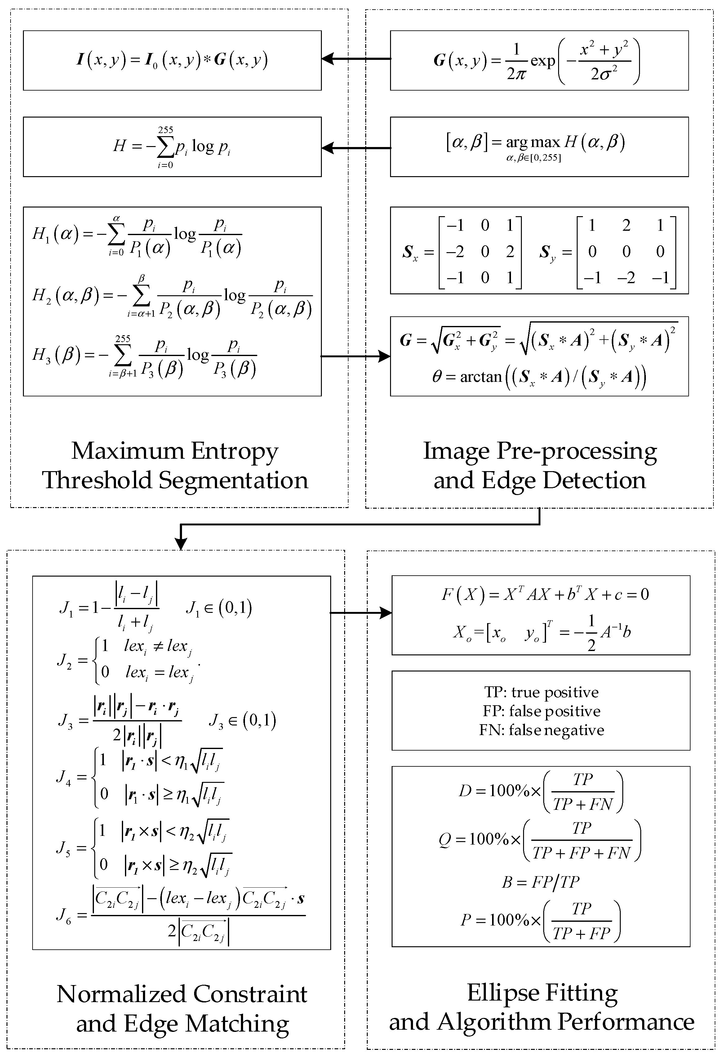
Crater detection based on maximum entropy thresholds (METS-CDA) and the ellipse fitting method proposed in Reference [8] are used as the sources of optical navigation information. The METS-CDA algorithm consists of four parts: maximum entropy threshold segmentation; image preprocessing and edge detection; normalized multi-index constraint matrix construction and edge matching; crater ellipse fitting and algorithm performance evaluation. As shown in Figure 1, the technical route of the METS-CDA method is briefly described below.

Firstly, the Gauss kernel function $G\left(x,y\right)$ was selected to preprocess the original image $I_o$, and, then, the image segmentation double threshold $\left[\alpha ,\beta \right]$, corresponding to the maximum information entropy, was calculated to complete the ternary image; on this basis, the crater edge detection was completed. 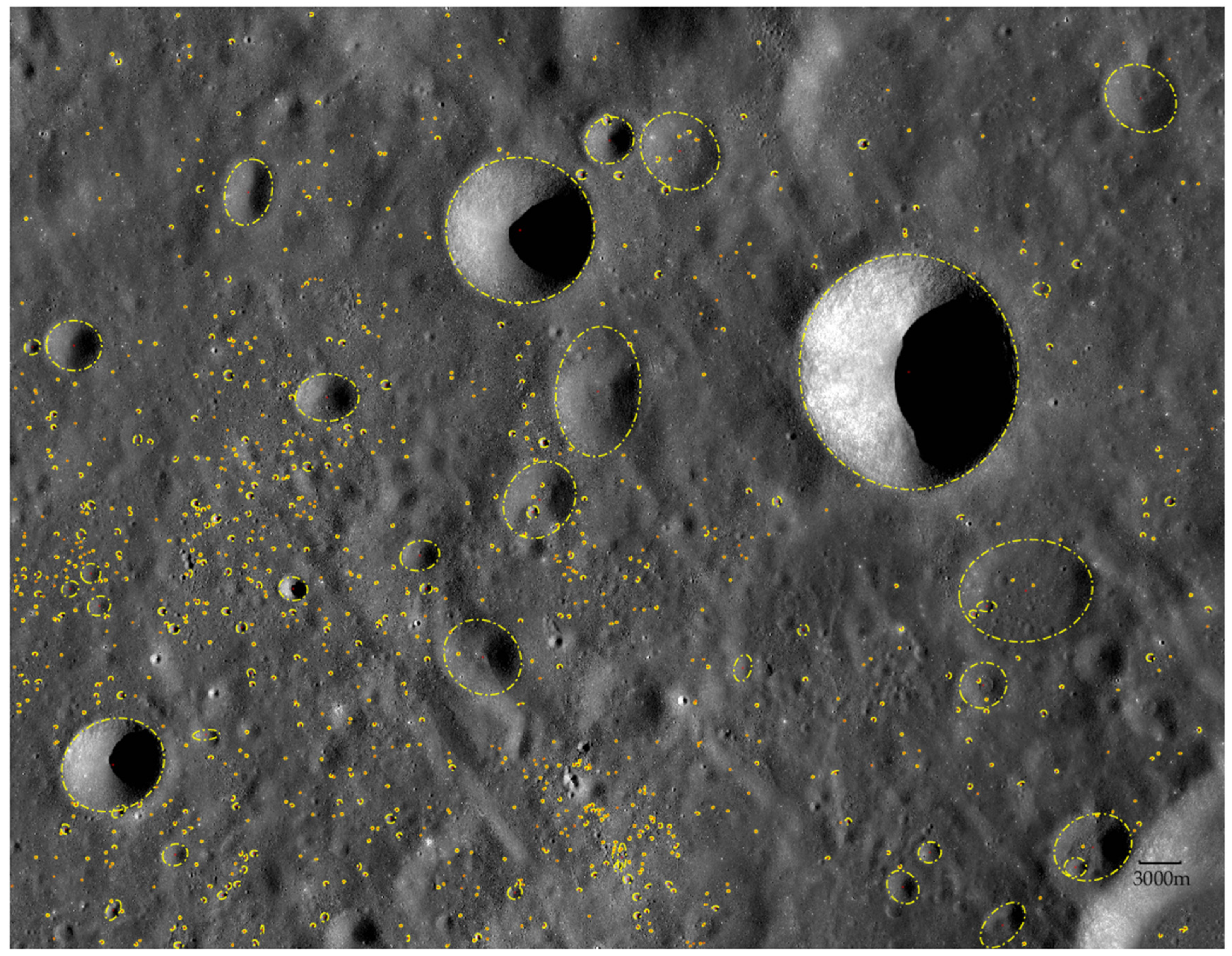The length, distance, light and shade, direction, and other information of the crater edge were comprehensively extracted, and a normalized multi-index constraint matrix $J_i\left(i=1,2\dots 6\right)$ was constructed to complete the crater edge matching. Finally, the crater ellipse fitting was carried out, and the quality of the crater was evaluated and extracted by quality parameters, such as detection rate D, detection quality Q, and branch factor B, and detection accuracy P. The results of the crater extraction are shown in Figure 2.

The lunar crater is modeled as an ellipse, which is described in Formula (1), and X is the gray coordinate point set at the edge of the crater:

$$F\left(X\right)=X^{\mathrm{T}}AX+b^{\mathrm{T}}X+1=0$$

(1)

$$X_i=\left[\begin{array}{c}{x}_i\\ y_i\end{array}\right],b=\left[\begin{array}{c}{\beta }_1\\ {\beta }_2\end{array}\right]$$

(2)

Due to the imaging error, there is an error between the coordinates of the edge of the crater obtained from the actual measurement and the coordinates of the real edge of the crater. Therefore, the actual measured coordinates of each point on the edge and the fitting equation are:

$$\tilde{F}\left(X\right)=X^{\mathrm{T}}AX+b^{\mathrm{T}}X+1=\epsilon$$

(3)

$${\tilde{X}}_i=\left[\begin{array}{c}{\tilde{x}}_i\\ {\tilde{y}}_i\end{array}\right]=\left[\begin{array}{c}{x}_i+\delta x\\ y_i+\delta y\end{array}\right]$$

(4)

The least squares method (LSM) is used to calculate the parameters A and b in Formula (3):

$$\begin{array}{cc}A=\left[\begin{array}{cc}{\alpha }_1& 0.5{\alpha }_2\\ 0.5{\alpha }_2& {\alpha }_4\end{array}\right]& b=\left[\begin{array}{c}{\beta }_1\\ {\beta }_2\end{array}\right]\end{array}$$

(5)

Construction of the ellipse coordinate matrix $H\left(\tilde{X}\right)$ is completed by using the following equation:

$$H_i\left(X_i\right)={\left[\begin{array}{lllll}{x}^2{}_i\hfill & x_i{y}_i\hfill & y^2{}_i\hfill & x_i\hfill & y_i\hfill \end{array}\right]}^{\mathrm{T}}$$

(6)

For the whole crater coordinate point set with errors $\tilde{X}$:

$$H\left(\tilde{X}\right)={\left[\begin{array}{cccc}{H}_1\left({\tilde{X}}_1\right)& H_2\left({\tilde{X}}_2\right)& \cdots & H_n\left({\tilde{X}}_n\right)\end{array}\right]}^{\mathrm{T}}$$

(7)

Bring (5), (6), and (7) into Formula (4) to obtain the ellipse fitting formula with error; := represents the definition of intermediate vector and matrix:

$$H\left(\tilde{X}\right){\left[\begin{array}{lllll}{\alpha }_1\hfill & {\alpha }_2\hfill & {\alpha }_4\hfill & {\beta }_1\hfill & {\beta }_2\hfill \end{array}\right]}^{\mathrm{T}}+1_{n\times 1}=H\left(\tilde{X}\right)\Theta \left(A,b\right)+1_{n\times 1}=\epsilon$$

(8)

The ellipse parameter vector $\Theta \left(A,b\right)$ of the crater is solved using the following equations:

$$\min J\left(\Theta \left(A,b\right)\right)={\epsilon }^{\mathrm{T}}\epsilon ={\left(H\left(\tilde{X}\right)\Theta \left(A,b\right)+1_{n\times 1}\right)}^{\mathrm{T}}\left(H\left(\tilde{X}\right)\Theta \left(A,b\right)+1_{n\times 1}\right)$$

(9)

$$\Theta \left(A,b\right)=-{\left(H^{\mathrm{T}}\left(\tilde{X}\right)H\left(\tilde{X}\right)\right)}^{-1}{H}^{\mathrm{T}}\left(\tilde{X}\right)1_{n\times 1}$$

(10)

The fitting ellipse center coordinates $X_o$ are:

$$X_o=\left[\begin{array}{c}{x}_o\\ y_o\end{array}\right]=-\frac{1}{2}{A}^{-1}b$$

(11)

3. Lander Optical Navigation Method Based on Crater-Detection Algorithm

3.1. Optical Navigation Imaging Measurement Model

After extracting the crater by the METS-CDA method, the position and attitude information of the lander (camera) can be calculated according to the relationship between the homogeneous imaging pixel system coordinates of the crater $P^{uv}$, the homogeneous coordinates of the planetary surface fixed geographical system of the center of the crater $P^f$, and the camera system coordinates $P^C$:

$$\left\{\begin{array}{l}{P}^{uv}={\left[\begin{array}{ccc}u& v& 1\end{array}\right]}^{\mathrm{T}}\\ P^f={\left[\begin{array}{cccc}{X}^f& Y^f& Z^f& 1\end{array}\right]}^{\mathrm{T}}\\ P^C={\left[\begin{array}{ccc}{X}^C& Y^C& Z^C\end{array}\right]}^{\mathrm{T}}\end{array}\right.$$

(12)

The direction cosine matrix from the lander body system $O_b-X_b{Y}_b{Z}_b$ to the planetary surface fixed geographical system $O_f-X_f{Y}_f{Z}_f$ is $C_b^f$, and the position of the lander under the geographical system is T:

$$C_f^b=\left[\begin{array}{ccc}{c}_{11}& c_{12}& c_{13}\\ c_{21}& c_{22}& c_{23}\\ c_{31}& c_{32}& c_{33}\end{array}\right]=\left[\begin{array}{c}{c}_1^T\\ c_2^T\\ c_3^T\end{array}\right],$$

(13)

$$T={\left[\begin{array}{ccc}{X}_C& Y_C& Z_C\end{array}\right]}^{\mathrm{T}}.$$

(14)

The imaging model of crater j is:

$$\begin{array}{cc}{U}_j=\frac{u_j}{f}=\frac{X_j^C}{Z_j^C},& V_j=\frac{v_j}{f}=\frac{Y_j^C}{Z_j^C}\end{array}.$$

(15)

where f is the focal length, and $X_j^C,Y_j^C$, and $Z_j^C$ are geographical system coordinates of crater j. Define the inhomogeneous imaging pixel system coordinates ${\tilde{P}}_j{}^{UV}$ of crater j:

$${\tilde{P}}_j{}^{UV}={\left[\begin{array}{cc}{U}_j& V_j\end{array}\right]}^{\mathrm{T}}.$$

(16)

Linking the lander pose information with the optical imaging:

$$\left[\begin{array}{c}{X}_j^C\\ Y_j^C\\ Z_j^C\end{array}\right]=\left[\begin{array}{ccc}{c}_{11}& c_{12}& c_{13}\\ c_{21}& c_{22}& c_{23}\\ c_{31}& c_{32}& c_{33}\end{array}\right]\left[\begin{array}{c}{X}_j^f\\ Y_j^f\\ Z_j^f\end{array}\right]+\left[\begin{array}{c}{X}_C\\ Y_C\\ Z_C\end{array}\right].$$

(17)

Rewrite the above formula into homogeneous form:

$$P^C=\left[C_f^b\left|T\right.\right]P_j^f.$$

(18)

The optical navigation of the lander, based on the CDA, is to obtain the values of Formulas (13) and (14), that is, to solve the 12 variables $\left[C_f^b\left|T\right.\right]$ in Formula (18).

Consider two kinds of constraints. For any crater j, simultaneous Formulas (15) and (17) can construct two of the first types of detection constraints ${\pi }_j{}^1$:

$${\pi }_j^1:\left\{\begin{array}{l}{U}_j=\frac{c_{11}{X}_j^f + c_{12}{Y}_j^f + c_{13}{Z}_j^f + X_C}{c_{31}{X}_j^f + c_{32}{Y}_j^f + c_{33}{Z}_j^f + Z_C}\\ V_j=\frac{c_{21}{X}_j^f + c_{22}{Y}_j^f + c_{23}{Z}_j^f + Y_C}{c_{31}{X}_j^f + c_{32}{Y}_j^f + c_{33}{Z}_j^f + Z_C}\end{array}\right..$$

(19)

Write Formula (19) into matrix form:

$$\left\{\begin{array}{c}\left[c_1^{\mathrm{T}}\left|X_C\right.\right]P_j^f-U_j\left[c_3^{\mathrm{T}}\left|Z_C\right.\right]P_j^f=0\\ \left[c_2^{\mathrm{T}}\left|Y_C\right.\right]P_j^f-V_j\left[c_3^{\mathrm{T}}\left|Z_C\right.\right]P_j^f=0\end{array}\right..$$

(20)

Rewriting Formula (20) with inhomogeneous coordinates of crater imaging:

$$⟮\left[\begin{array}{cc}{c}_1^{\mathrm{T}}& X_C\\ c_2^{\mathrm{T}}& Y_C\end{array}\right]P_j^f-P_j^{UV}\left[c_3^{\mathrm{T}}\left|Z_C\right.\right]⟯P_j^f=0.$$

(21)

The second type of constraint ${\pi }^2$ is the directional cosine matrix constraint:

$${\left(C_f^b\right)}^{\mathrm{T}}{C}_f^b=I.$$

(22)

To reduce the computational complexity, the traditional optical navigation method usually carries out the navigation solution after identifying and selecting four craters. The corresponding constraint ${\pi }_j{}^1$ is:

$${\pi }_{j=1:4}^1\left(\left[C_f^b\left|T\right.\right]\right)=\mathbf{0}.$$

(23)

Supplementary formula ${\pi }^2$:

$${\pi }^2\left(\left[C_f^b\left|T\right.\right]\right)=\left[\begin{array}{c}{c}_1^{\mathrm{T}}{c}_1-1\\ c_2^{\mathrm{T}}{c}_2-1\\ c_3^{\mathrm{T}}{c}_3-1\\ c_1^{\mathrm{T}}{c}_2\end{array}\right]=\mathbf{0}.$$

(24)

The simultaneous two types of constraints ${\pi }^1$ and ${\pi }^2$ are as follows:

$$\pi \left(\left[C_f^b\left|T\right.\right]\right)=\left[\begin{array}{c}{\pi }^1\left(\left[C_f^b\left|T\right.\right]\right)\\ {\pi }^2\left(\left[C_f^b\left|T\right.\right]\right)\end{array}\right]=\mathbf{0}.$$

(25)

$${\pi }_k=\pi \left({\left[C_f^b\left|T\right.\right]}_k\right),$$

(26)

Formula (26) can be solved by the Gauss–Newton method:

$${\left[C_f^b\left|T\right.\right]}_{k+1}={\left[C_f^b\left|T\right.\right]}_k-{\pi }_k{⟮\frac{\partial {\pi }_k}{\partial {\left[C_f^b\left|T\right.\right]}_k}⟯}^{-1}.$$

(27)

3.2. Improved Gradient Descent Method in OPNAV

Formula (27) usually converges slowly. To solve this problem, an improved gradient descent (IGD) method is proposed. The gradient of the solution objective function is constructed as follows:

$$J\left(\left[C_f^b\left|T\right.\right]\right)=\frac{1}{2}{\left(\begin{array}{c}{\pi }_{j=1:3}^1\\ {\pi }^2\end{array}\right)}^T\left(\begin{array}{c}{\pi }_{j=1:3}^1\\ {\pi }^2\end{array}\right).$$

(28)

Design the iteration step $\lambda$ and direction $g$ of the improved gradient descent method:

$$\lambda =\left\{\begin{array}{cc}{\lambda }_0& J\left({\left[C_f^b\left|T\right.\right]}_{k+1}\right)-J\left({\left[C_f^b\left|T\right.\right]}_k\right)\le 0\\ 0.5*\lambda & J\left({\left[C_f^b\left|T\right.\right]}_{k+1}\right)-J\left({\left[C_f^b\left|T\right.\right]}_k\right)>0\end{array}\right.,$$

(29)

$$g=\frac{\partial \pi \left(\left[C_f^b\left|T\right.\right]\right)}{\partial \left[C_f^b\left|T\right.\right]}+\left(J\left({\left[C_f^b\left|T\right.\right]}_{k+1}\right)-J\left({\left[C_f^b\left|T\right.\right]}_k\right)\right){\widehat{g}}_{\perp }.$$

(30)

The value ${\lambda }_0$ is the initial iteration step size, and ${\widehat{g}}_{\perp }$ is the vertical vector of the iteration direction of the previous step. The improved gradient descent formula is shown in Formula (31).

$${\left[C_f^b\left|T\right.\right]}_{k+1}={\left[C_f^b\left|T\right.\right]}_k-\lambda g.$$

(31)

Compared with Formula (27), Formula (31) can significantly improve the solution speed.

When more than four craters are detected at the same time, there are two methods to solve the position and attitude of the aircraft. The first method is to comprehensively consider the detection information of all craters and obtain the optimal solution that conforms to all imaging relations. The second method is to select four optimal craters from all detected craters for solution.

When the first method is adopted, the variable covariance matrix Q is introduced to Formula (28), to improve the objective function. The new objective function is:

$$J\left(\left[C_f^b\left|T\right.\right]\right)=\frac{1}{2}{\left(\begin{array}{c}{\pi }_{j=1:3}^1\\ {\pi }^2\end{array}\right)}^{T}Q\left(\begin{array}{c}{\pi }_{j=1:3}^1\\ {\pi }^2\end{array}\right).$$

(32)

The variable covariance matrix Q is shown in Formula (33), which is the crater detection reliability matrix, and n is the number of detected craters. The value ${\Sigma }_{2n\times 2n}$ is a diagonal matrix, and each element in the diagonal matrix is the corresponding covariance of the craters.

$$Q=\mathrm{blkdiag}\left[{\Sigma }_{2n\times 2n},I_{6\times 6}\right]$$

(33)

$$\begin{array}{cc}{\Sigma }_{2n\times 2n}=\mathrm{diag}\left[{\sigma }_i^2\right]& i=1,2,\cdots ,n\end{array}$$

(34)

This method enlarges the dimension of the formula, increases the complexity of solving the formula, and reduces the real-time performance of the navigation system.

3.3. Spatial Positioning Distribution Model of Torus-OPNAV

The traditional lander positioning method based on optical crater detection information usually needs to detect four craters to complete the navigation solution. When the number of detected craters is less than 4, the observation vector corresponding to the detected craters is often taken as the analysis object, and the observation vector error is taken as the observation to construct the error transfer formula for navigation. This kind of optical navigation method has three disadvantages:

(1) When the number of the reference feature terrain is less than 3, the calculation results of the optical navigation system may not converge.

(2) The detection information of the detected craters is not fully utilized, and the spatial position distribution and other information contained in the optical imaging mathematical model are not fully analyzed.

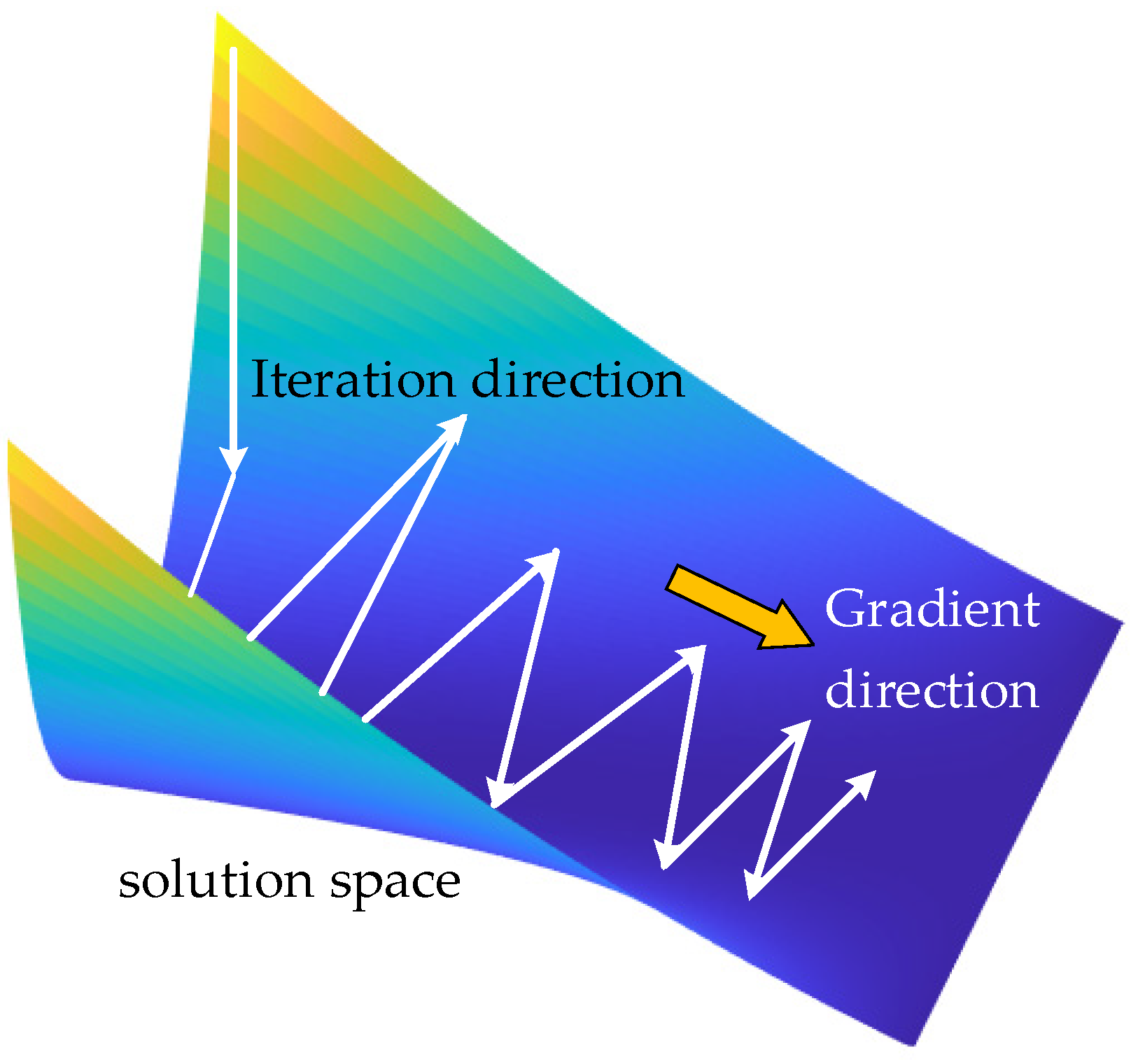
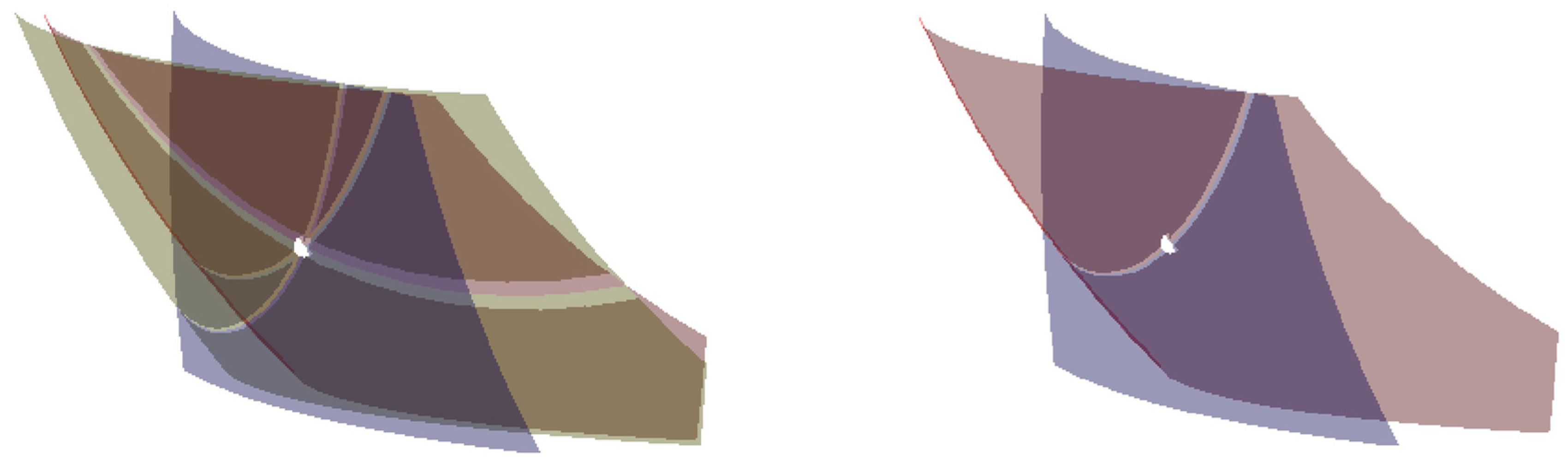
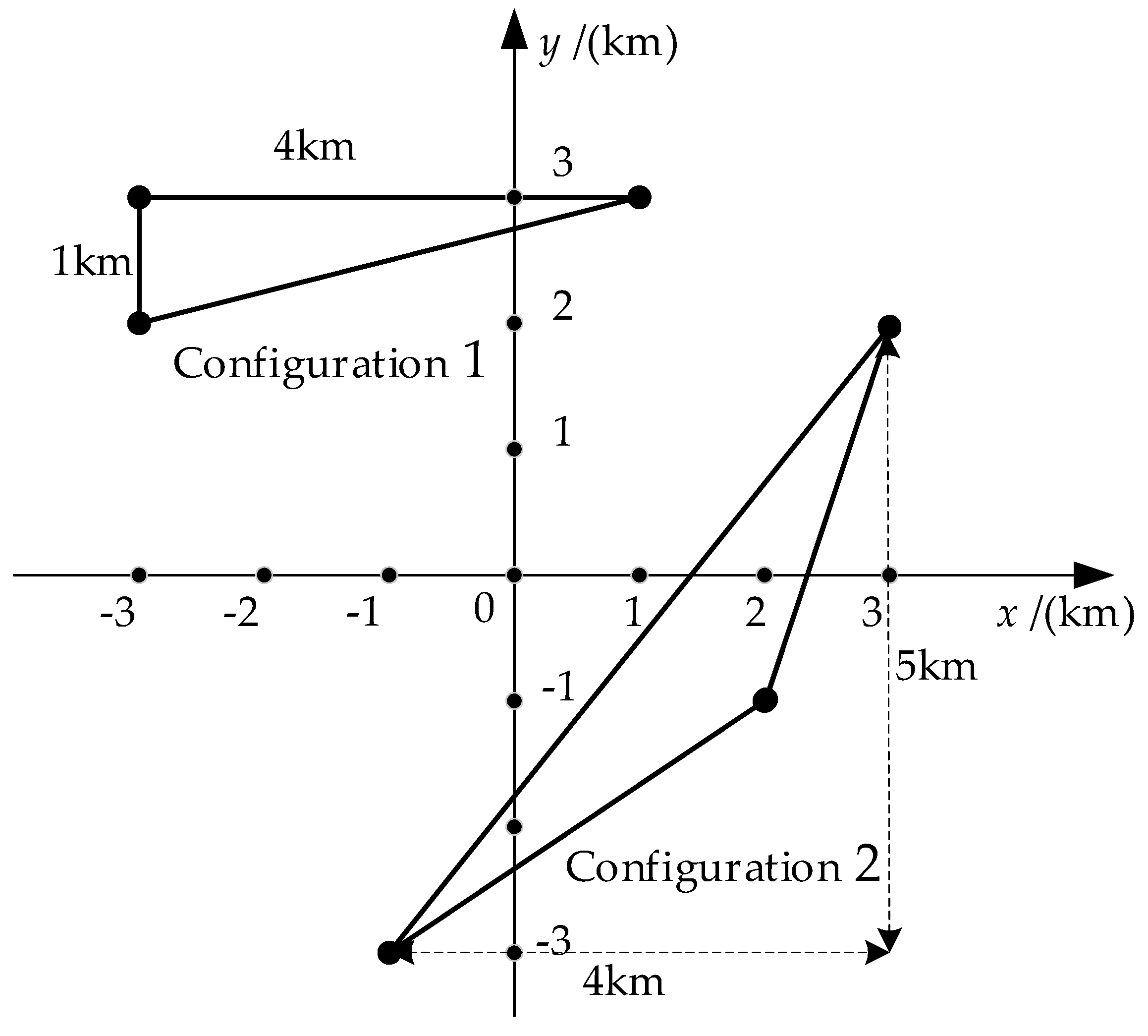
(3) Under some observation conditions, the solution space of lander position solution may be flat, as shown in Figure 3, which brings challenges to iterative solution methods, such as the gradient descent (GD) method.

In addition, to improve the efficiency of the navigation system, when there are many detected craters and other terrain characteristics, it is necessary to select several craters from all the detected craters for optical navigation, which may mean the optical navigation solution is unable to reach an optimal result. Ref. [13] analyzed the infimum of optical navigation position estimation error under the condition of n detected craters by calculating the Fisher information matrix and the Cramér–Rao bound:

$$\frac{3}{\mathrm{tr}\left(F^n\right)}=\frac{3{\left({\sigma }_u{z}^c\right)}^2}{2n{f}^2+{\displaystyle \sum _{i=1}^n\left(u_i^2+v_i^2\right)}}.$$

(35)

In Formula (29), $F^n$ is the Fisher information matrix, ${\sigma }_u$ is the measurement noise variance, $z^c$ is the z-direction projection of the observation feature in the camera system coordinate system, f is the focal length of the navigation camera (NAVCam), and $\left[u_i,v_i\right]$ are the imaging coordinates of the observation feature. Formula (29) shows that when the lander height is constant, the lower bound of position estimation error decreases with the increase in the number of detection characteristics. In actual engineering, geometric distribution method, or information entropy method are usually used to select several optimal craters for a navigation solution, so the infimum by $F^n$ of error makes it difficult to meet the design requirements of the navigation system. Therefore, it is necessary to fully mine the optical detection information and analyze the general form of error propagation characteristics.

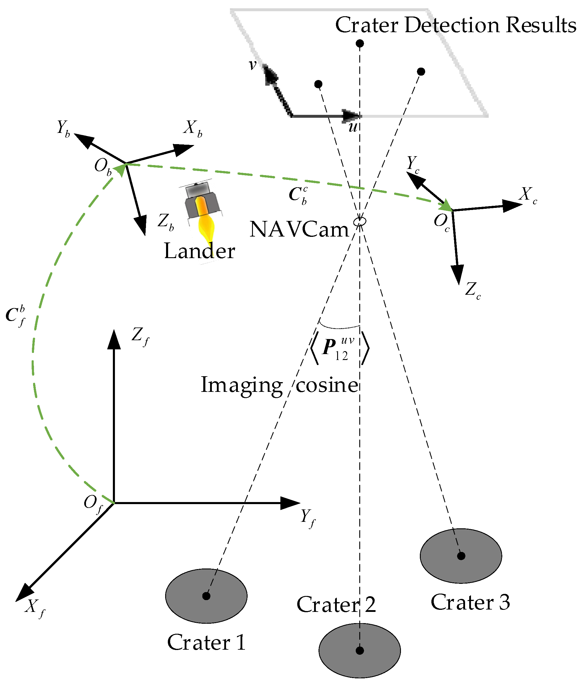
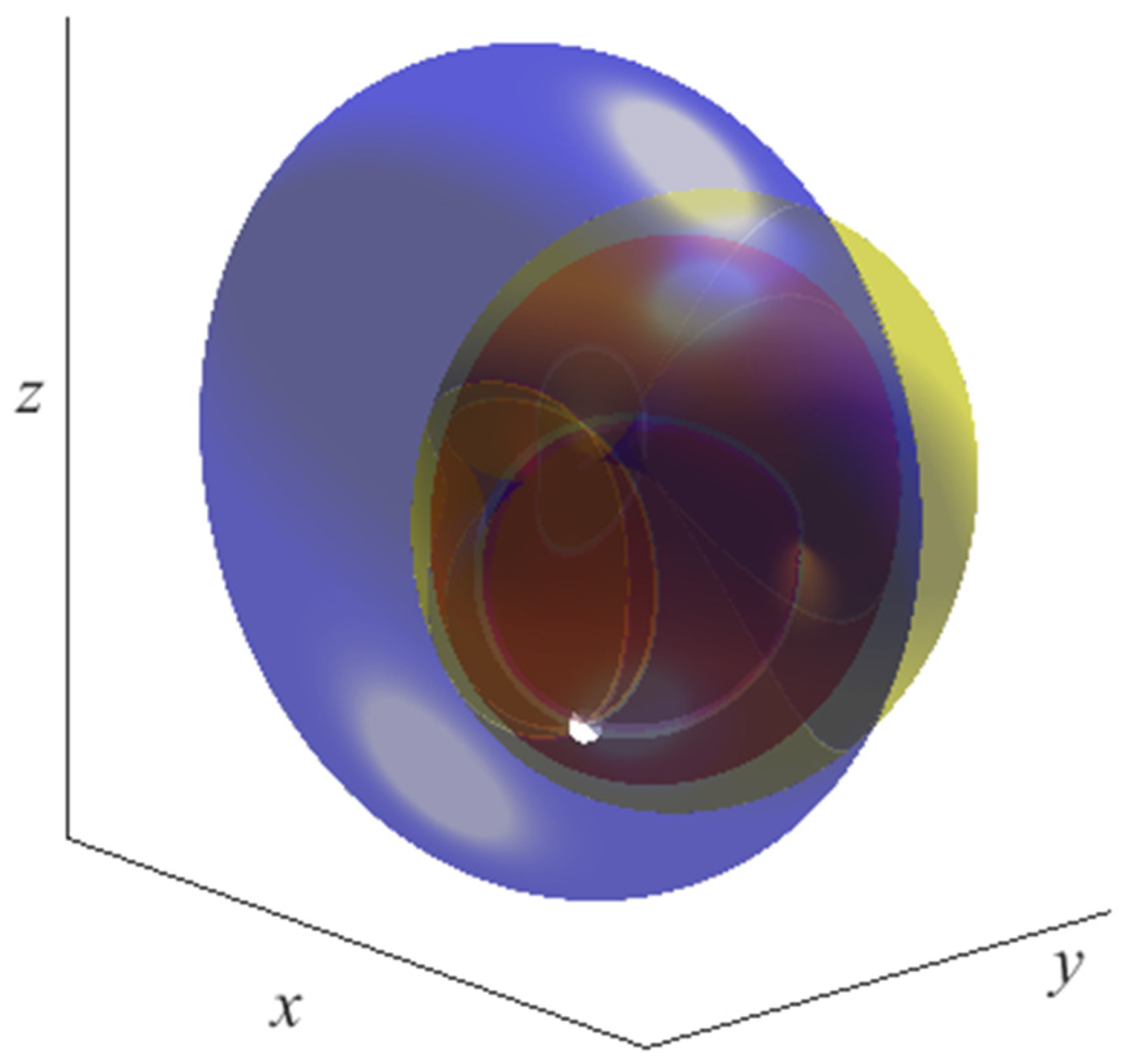
An OPNAV algorithm independent of the observation vector of the crater is constructed, as shown in Figure 4. The figure depicts the planetary surface fixed geographic coordinate system $O_f-X_f{Y}_f{Z}_f$, body coordinate system $O_b-X_b{Y}_b{Z}_b$, camera system coordinate system $O_C-X_C{Y}_C{Z}_C$, imaging coordinate system $o-uv$, and their attitude conversion relationships used in the optical navigation system. After successful detection, the craters are projected onto the image plane, and the imaging cosine equivalent model between objects and images is established to realize optical navigation attitude determination and position determination.

When the optical NAVCam of the lander detects any two craters $P_{i,j}^{}$, the imaging cosine $〈P_{i,j}^{UV}〉$ of the two craters in the image coordinate system is:

$$〈P_{i,j}^{UV}〉=\frac{U_i{U}_j+V_i{V}_j+1}{\sqrt{U_i^2+V_i^2+1}\sqrt{U_j^2+V_j^2+1}}.$$

(36)

At the same time, considering the inhomogeneous coordinates ${\tilde{P}}_{i,j}^f$ of the craters and the position coordinates $r$ of the lander in the geographical system:

$$〈P_{i,j}^{UV}〉=\frac{r^2-2\left({\tilde{P}}_i^f+{\tilde{P}}_j^f\right)r+{\tilde{P}}_i^f{\tilde{P}}_j^f}{\left|r-{\tilde{P}}_i^f\right|\left|r-{\tilde{P}}_j^f\right|},{\tilde{P}}_{i,j}^f={\left[\begin{array}{ccc}{X}^f& Y^f& Z^f\end{array}\right]}^{\mathrm{T}}.$$

(37)

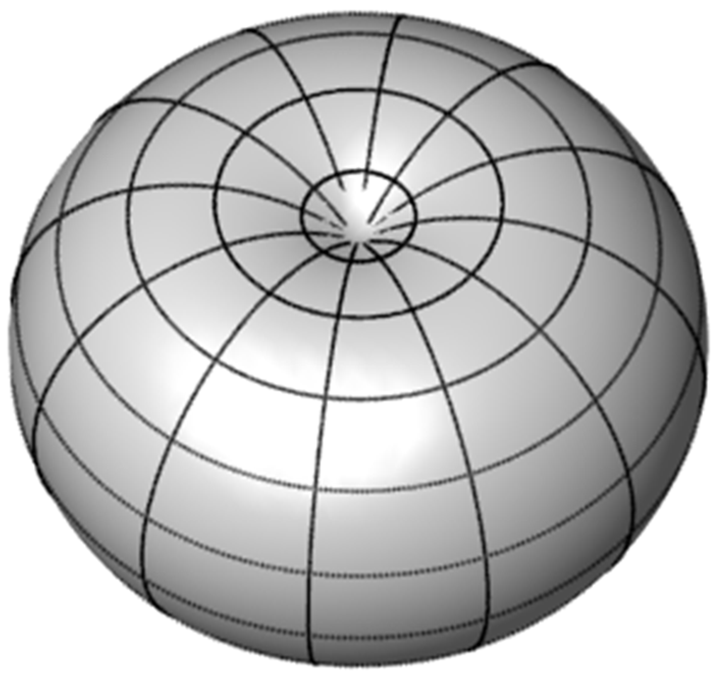
When only two craters are observed, although the lander position cannot be solved, Formulas (36) and (37) reflect the spatial position distribution of the lander in the geographical system, and the lander exists in the spatial position distribution surface described in Figure 5.

The surface described in Figure 5 is a torus. It is defined as the product of two circles and is an Abelian Lie group [20]:

$$S^1\times L^1=T^2$$

(38)

Torus in optical navigation can be obtained from a set of parametric Formula (39). The parametric formula consists of two parts: the point set $P_l\in \mathbb{L}$, describing the circle $L$ in space; and the point set $P_s\in \mathbb{S}$, describing the surface $S$ where the lander is located in space:

$$\left\{\begin{array}{l}L:\left\{\begin{array}{c}\left|2P_l-\left({\tilde{P}}_i^f+{\tilde{P}}_j^f\right)\right|=d{\tan }^{-1}〈P_{i,j}^{UV}〉\\ \left(2P_l-\left({\tilde{P}}_i^f+{\tilde{P}}_j^f\right)\right)•\left({\tilde{P}}_i^f-{\tilde{P}}_j^f\right)=0\end{array}\right.\hfill \\ S:2\left|\left(P_s-P_l\right)\right|\sin 〈P_{i,j}^{UV}〉=d\hfill \end{array}\right.$$

(39)

In Formula (39), d is the Euclidean distance between two craters. When given a pair of crater detection results or an imaging cosine, the spatial position distribution of the lander can be accurately described mathematically. We avoid introducing the calculation of formulas such as Gauss–Newton, GD or IGD and reduce the amount of calculation.

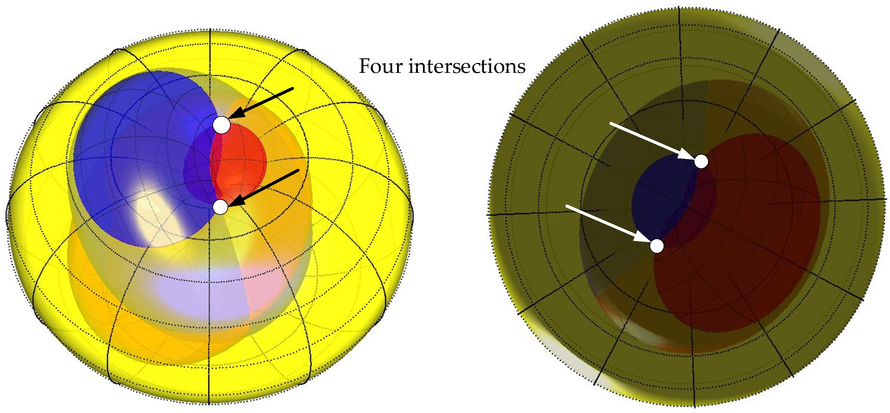
When three craters are given, three sets of constraints $\left\{L,S\right\}$ can be constructed to numerically solve the position P of the lander:

$$P={\left\{L,S\right\}}_{12}\cap {\left\{L,S\right\}}_{13}\cap {\left\{L,S\right\}}_{23}$$

(40)

Four solutions $\begin{array}{cc}{\Lambda }^i& \left(i=1,2,3,4\right)\end{array}$ conforming to the constraints can be obtained from three sets of constraints. As shown in Figure 6, the lander must be in the position of one of the solutions. Combined with the height constraint $h>0$ and the velocity direction constraint, the position $P_k$ of the lander at time k can be uniquely determined:

$$\begin{array}{l}{P}_k=\mathrm{argmin}\left(\mathcal{X}\left(\Lambda \right)+\mathcal{X}\left(P\right)\right)\\ =\begin{array}{cc}\mathrm{argmin}{‖\left({\Lambda }_k^i-{\Lambda }_{k-1}^i\right)+\left(P_k^{}-P_{k-1}^{}\right)‖}_2& i=1,2,3,4\end{array}\end{array}$$

(41)

$${\left[P_k\right]}_z=h\ge 0$$

(42)

In Formula (41), $\mathcal{X}\left(\Lambda \right)$ is an objective function of solution ${\Lambda }^i$, $\mathcal{X}\left(P\right)$ is an objective function of the position.

After the position of the planetary lander is solved, the attitude is solved by using its coordinate information. According to Formula (17), after the lander position information is given, the attitude information is decoupled from the positioning result and can be calculated directly. Considering all the geographical system coordinates ${\tilde{P}}^f$ and camera system coordinates $P^C$ of the crater during the imaging process, the following conversion relations exist between them:

$$P_{}^C=C_f^C{\tilde{P}}_{}^f=C_f^b\left({\tilde{P}}_{}^f+r\right)=C_f^b{\overline{P}}_{}^f.$$

(43)

where ${\overline{P}}_{}^f$ is the augmented homogeneous geographical system coordinate:

$${\overline{P}}_{}^f={\tilde{P}}_{}^f+r.$$

(44)

The lander attitude is:

$$C_f^b=P_{}^C{\left({\overline{P}}_{}^f\right)}^{\mathrm{T}}{\left({\overline{P}}_{}^f{\left({\overline{P}}_{}^f\right)}^{\mathrm{T}}\right)}^{-1}.$$

(45)

4. Torus-OPNAV Error Analysis and Its Influence

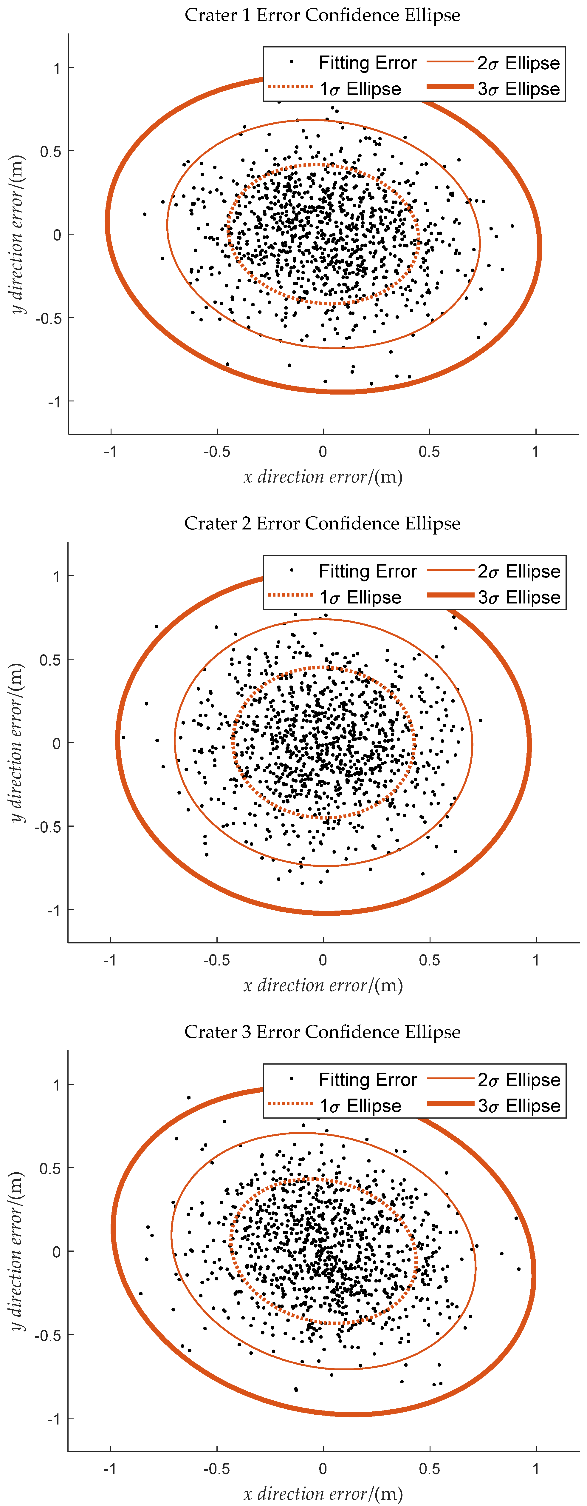
By analyzing Formulas (1) and (3), due to the detection error, the extracted crater edge does not necessarily coincide with the real edge, so the crater ellipse fitting also produces errors. Crater fitting error directly reflects the influence of detection error.

The essence of the CDA-OPNAV method is to fit the crater ellipse formula and calculate the ellipse center coordinates through the least squares algorithm when the crater is detected, analyze the mathematical relationship between the image point coordinates and the camera system coordinates in the imaging process of the ellipse center, and complete the lander navigation solution.

4.1. Error Analysis of Crater Ellipse Fitting

The detection error of crater obeys normal distribution:

$$\begin{array}{cc}{\tilde{X}}_i={\left[\begin{array}{cc}{\tilde{x}}_i& {\tilde{y}}_i\end{array}\right]}^{\mathrm{T}}=X_i+{\upsilon }_i& {\upsilon }_i\sim \mathcal{N}\left(0,R_{X_i{X}_i}\right)\end{array}$$

(46)

For one point on the crater ${\tilde{X}}_i$, the imaging error is:

$$\epsilon \left({\tilde{X}}_i\right)={\epsilon }_i=H_i\left({\tilde{X}}_i\right)\Theta \left(A,b\right)+1_{n\times 1}.$$

(47)

The Taylor expansion of Formula (47) is as follows:

$$\epsilon \left({\tilde{X}}_i\right)=\epsilon \left(X_i\right)+\frac{\partial \epsilon \left(X_i\right)}{\partial X_i}\left({\tilde{X}}_i-X_i\right)+O\left(\delta X_i\right),$$

(48)

where $O\left(\delta X_i\right)$ is the higher-order infinitesimal of $\delta X_i$. Only the first-order term of Formula (48) is considered:

$$\delta {\epsilon }_i=\epsilon \left({\tilde{X}}_i\right)-\epsilon \left(X_i\right)=\frac{\partial \epsilon \left(X_i\right)}{\partial X_i}\left({\tilde{X}}_i-X_i\right)=\frac{\partial {\epsilon }_i}{\partial X_i}\delta X_i.$$

(49)

Substitute Formulas (3) and (5) into Formula (49):

$$\frac{\partial \epsilon \left(X_i\right)}{\partial X_i}={\left[\begin{array}{c}2{\alpha }_1{x}_i+{\alpha }_2{y}_i+{\beta }_1\\ {\alpha }_2{x}_i+2{\alpha }_4{y}_i+{\beta }_2\end{array}\right]}^{\mathrm{T}}.$$

(50)

Then, the observation residual variance of the crater is:

$${\sigma }_i^2=\mathrm{E}\left[\delta {\epsilon }_i^2\right]=\frac{\partial {\epsilon }_i}{\partial X_i}\mathrm{E}\left[\delta X_i\delta X_i^{\mathrm{T}}\right]\frac{\partial {\epsilon }_i{}^{\mathrm{T}}}{\partial X_i}=\frac{\partial {\epsilon }_i}{\partial X_i}{R}_{X_i{X}_i}\frac{\partial {\epsilon }_i{}^{\mathrm{T}}}{\partial X_i}.$$

(51)

Next, the influence of the single point observation error of the crater on the crater ellipse fitting is calculated. Substituting error Formula (51) into Formula (8), solve the ellipse coordinate matrix with errors $H_i\left({\tilde{X}}_i\right)$, separate the errors and ignore the higher-order error term:

$$H_i\left({\tilde{X}}_i\right)=\left[\begin{array}{c}{x}_i^2+2x_i\delta x_i{}^2\\ x_i{y}_i+x_i\delta y_i+y_i\delta x_i\\ y_i^2+2y_i\delta y_i\\ x_i+\delta x_i\\ y_i+\delta y_i\end{array}\right]=\left[\begin{array}{c}{x}_i^2\\ x_i{y}_i\\ y_i^2\\ x_i\\ y_i\end{array}\right]+\left[\begin{array}{c}\begin{array}{cc}2x_i& 0\end{array}\\ \begin{array}{cc}{y}_i& x_i\end{array}\\ \begin{array}{cc}0& 2y_i\end{array}\\ I_2\end{array}\right]\left[\begin{array}{c}\delta x_i\\ \delta y_i\end{array}\right]:=H_i\left(X_i\right)+E\delta X_i.$$

(52)

Substituting Formula (52) into Formulas (9) and (10), the least squares estimation of the crater parameter vector $\widehat{\Theta }\left(\widehat{A},\widehat{b}\right)$ with error is:

$$\widehat{\Theta }\left(\widehat{A},\widehat{b}\right)=-{\left(H{\left(\tilde{X}\right)}^{\mathrm{T}}H\left(\tilde{X}\right)\right)}^{-1}H{\left(\tilde{X}\right)}^{\mathrm{T}}{1}_{n\times 1}.$$

(53)

Let $H=H\left(X\right)$, $K:={\left(H^{\mathrm{T}}H\right)}^{-1}$, ignore the higher-order error term, and simplify Formula (53):

$$\begin{array}{l}\widehat{\Theta }\left(\widehat{A},\widehat{b}\right)=-{\left({\left(H\left(X\right)+E\delta X\right)}^{\mathrm{T}}\left(H\left(X\right)+E\delta X\right)\right)}^{-1}{\left(H\left(X\right)+E\delta X\right)}^{\mathrm{T}}{1}_{n\times 1}\\ =-{\left(H^{\mathrm{T}}H\right)}^{-1}{H}^{\mathrm{T}}{1}_{n\times 1}+\left(\left(H^{\mathrm{T}}E\delta X+\delta X^{\mathrm{T}}{E}^{\mathrm{T}}H\right)H^{\mathrm{T}}-K\delta X^{\mathrm{T}}{E}^{\mathrm{T}}\right)1_{n\times 1}\\ =\Theta \left(A,b\right)+\left(\left(H^{\mathrm{T}}E\delta X+\delta X^{\mathrm{T}}{E}^{\mathrm{T}}H\right)H^{\mathrm{T}}-K\delta X^{\mathrm{T}}{E}^{\mathrm{T}}\right)1_{n\times 1}.\end{array}$$

(54)

According to the comparison between Formula (54) and Formula (10), $\hat{\Theta }\left(\hat{A},\hat{b}\right)$ is composed of two parts: one is the least squares term without error $\Theta \left(A,b\right)$, and the other is the error term.

From:

$$H\left(X\right)\hat{\Theta }\left(\hat{A},\hat{b}\right)={\epsilon }_i-1_{n\times 1},$$

(55)

$$\hat{\Theta }\left(\hat{A},\hat{b}\right)={\left(H^{\mathrm{T}}H\right)}^{-1}{H}^{\mathrm{T}}\left({\epsilon }_i-1_{n\times 1}\right),$$

(56)

the error term $\delta \hat{\Theta }$ is:

$$\delta \hat{\Theta }\left(\hat{A},\hat{b}\right)={\left(H^{\mathrm{T}}H\right)}^{-1}{H}^{\mathrm{T}}\delta \epsilon =K{H}^{\mathrm{T}}\delta \epsilon .$$

(57)

Thus, the error distribution ${\sigma }_{\Theta }^2$ of $\hat{\Theta }\left(\hat{A},\hat{b}\right)$ is:

$$\begin{array}{c}{\sigma }_{\Theta }^2=\mathrm{E}\left[\delta {\hat{\Theta }}^2\right]=K{H}^{\mathrm{T}}\mathrm{E}\left[\delta \epsilon \delta {\epsilon }_{}^{\mathrm{T}}\right]H{K}^{\mathrm{T}}=K{H}^{\mathrm{T}}\Sigma H{K}^{\mathrm{T}}.\\ \begin{array}{cc}\Sigma =\mathrm{diag}\left[{\sigma }_i^2\right]& i=1,2,\cdots n\end{array}\end{array}$$

(58)

The center coordinate of the measured crater after correction is:

$$\begin{array}{c}{\hat{X}}_o=\left[\begin{array}{c}{\hat{x}}_o\\ {\hat{y}}_o\end{array}\right]=X_o-\delta X_o=-\frac{1}{2}{\left(A+\delta A\right)}^{-1}\left(b+\delta b\right).\\ \left(\delta A,\delta b\right)=⟮\left[\begin{array}{cc}\delta \Theta \left(1,1\right)& \frac{1}{2}\delta \Theta \left(2,1\right)\\ \frac{1}{2}\delta \Theta \left(2,1\right)& \delta \Theta \left(3,1\right)\end{array}\right],\left[\begin{array}{c}\delta \Theta \left(4,1\right)\\ \delta \Theta \left(5,1\right)\end{array}\right]⟯\sim \mathcal{N}\left(0,{\sigma }_{\Theta }^2\right)\end{array}$$

(59)

4.2. Crater Ellipse Fitting Error Influence on Position Determination

Due to the crater ellipse fitting error, the ellipse center imaging does not necessarily correspond to the real crater center coordinates. In other words, the pixel system coordinates $P^{uv}$ of the central point of the crater photographed by the optical navigation camera also have errors, as shown in Formula (60):

$$\left(P^{uv}\right)\prime =\left[\begin{array}{ccc}u\prime & v\prime & 1\end{array}\right]={\hat{P}}^{uv}+\delta P^{uv}.$$

(60)

where ${\hat{P}}^{uv}$ is the true value of the ellipse center imaging system coordinates. Substituting Formula (60) into Formula (15), the imaging model of crater j considering error is:

$$\left\{\begin{array}{c}U{\prime }_j=\frac{u{\prime }_j}{f}=\frac{X_j^C + \delta X_j^C}{Z_j^C + \delta Z_j^C}\\ V{\prime }_j=\frac{v{\prime }_j}{f}=\frac{Y_j^C + \delta Y_j^C}{Z_j^C + \delta Z_j^C}\end{array}\right..$$

(61)

Analyze Formula (61) and separate its error:

$$\begin{array}{l}{U}_j\prime =\frac{X_j^C+\delta X_j^C}{Z_j^C+\delta Z_j^C}=\frac{1}{Z_j^C}\left(X_j^C+\delta X_j^C\right){\left(1+\frac{\delta Z_j^C}{Z_j^C}\right)}^{-1}\\ =\frac{1}{Z_j^C}\left(X_j^C+\delta X_j^C\right)\left(1-\frac{\delta Z_j^C}{Z_j^C}\right)\\ =U_j+\frac{1}{Z_j^C}\delta X_j^C+\frac{X_j^C}{{\left(Z_j^C\right)}^2}\delta Z_j^C.\end{array}$$

(62)

For the same reason:

$$V_j\prime =V_j+\frac{1}{Z_j^C}\delta Y_j^C+\frac{Y_j^C}{{\left(Z_j^C\right)}^2}\delta Z_j^C.$$

(63)

Therefore, the imaging pixel system coordinates of the center of the crater j considering the error are:

$$\left({\tilde{P}}_j^{UV}\right)\prime =\left[\begin{array}{c}{U}_j\\ V_j\end{array}\right]+\left[\begin{array}{lll}\frac{1}{Z_j^C}\hfill & 0\hfill & \frac{X_j^C}{{\left(Z_j^C\right)}^2}\hfill \\ 0\hfill & \frac{1}{Z_j^C}\hfill & \frac{Y_j^C}{{\left(Z_j^C\right)}^2}\hfill \end{array}\right]\left[\begin{array}{c}\delta X_j^C\\ \delta Y_j^C\\ \delta Z_j^C\end{array}\right]:={\tilde{P}}_j^{UV}+W_j\delta X_o.$$

(64)

The error distribution of $\delta {\tilde{P}}_j^{UV}$ is:

$$\delta {\tilde{P}}_j^{UV}=\left({\tilde{P}}_j^{UV}\right)\prime -{\tilde{P}}_j^{UV}=W_j\delta X_o,$$

(65)

$${\sigma }_{P^{UV}}^2=\mathrm{E}\left[{\left(\delta {\tilde{P}}_j^{UV}\right)}^2\right]=W_j\mathrm{E}\left[\delta X_o\delta X_o^T\right]W_j{}^{\mathrm{T}}.$$

(66)

Calculate $\mathrm{E}\left[\delta X_o\delta X_o^T\right]$ according to Formula (59) and ignore the higher-order error term in the above formula:

$$\begin{array}{l}{\hat{X}}_o=-\frac{1}{2}{\left(A+\delta A\right)}^{-1}\left(b+\delta b\right)\\ =-\frac{1}{2}{A}^{-1}{\left(I+A^{-1}\delta A\right)}^{-1}\left(b+\delta b\right)\\ =-\frac{1}{2}{A}^{-1}b+\frac{1}{2}{A}^{-1}\left[\begin{array}{cc}{A}^{-1}b& -1\end{array}\right]\left[\begin{array}{c}\delta A\\ \delta b\end{array}\right]\\ :=X_o+M\left(\hat{\Theta }\right)\delta \hat{\Theta }\left(\hat{A},\hat{b}\right).\end{array}$$

(67)

The crater ellipse parameter vector $\Theta \left(A,b\right)$ is introduced to rewrite the matrix, as shown in Formula (68):

$$\frac{1}{2}{A}^{-1}\left[\begin{array}{cc}{A}^{-1}b& -1\end{array}\right]\left[\begin{array}{c}\delta A\\ \delta b\end{array}\right]:=M\left(\delta \Theta \right)\delta \hat{\Theta }$$

(68)

Therefore:

$$\delta X_o={\hat{X}}_o-X_o=M\left(\hat{\Theta }\right)\delta \hat{\Theta }\left(\hat{A},\hat{b}\right)=M\delta \hat{\Theta },$$

(69)

$${\sigma }_{X_o}^2=\mathrm{E}\left[\delta X_o^2\right]=M\mathrm{E}\left[\delta \hat{\Theta }\delta {\hat{\Theta }}^T\right]M^{\mathrm{T}}=M{\sigma }_{\Theta }^2{M}^{\mathrm{T}}.$$

(70)

Substitute ${\sigma }_{X_o}^2$ into ${\sigma }_{P^{UV}}^2$:

$${\sigma }_{P^{UV}}^2=W\mathrm{E}\left[\delta X_o\delta X_o^T\right]W^{\mathrm{T}}=W{\sigma }_{X_o}^2{W}^{\mathrm{T}}=WM{\sigma }_{\Theta }^2{M}^{\mathrm{T}}{W}^{\mathrm{T}}.$$

(71)

Next, use ${\sigma }_{P^{UV}}^2$ to calculate error variance of imaging cosine ${\sigma }^2\left(〈P_{i,j}^{UV}〉\right)$. Define intermediate parameters without errors $t_i$,$t_j$ and $g_{i,j}$:

$$\left\{\begin{array}{c}{t}_i:=1+U_i^2+V_i^2\\ t_j:=1+U_j^2+V_j^2\\ g_{i,j}:=1+U_i{U}_j+V_i{V}_j\end{array}\right.$$

(72)

Define intermediate parameters with errors ${\lambda }_{i,j}$, ${\gamma }_{i,j}$ and $\varphi$:

$${\gamma }_{i,j}:=\frac{U_{i,j}}{t_{i,j}}\delta U_{i,j}+\frac{V_{i,j}}{t_{i,j}}\delta V_{i,j},$$

(73)

$${\lambda }_{i,j}:={\left(t_{i,j}+2U_{i,j}\delta U_{i,j}+2V_{i,j}\delta V_{i,j}\right)}^{-\frac{1}{2}}:=t_{i,j}^{-\frac{1}{2}}\left(1-{\gamma }_{i,j}\right),$$

(74)

$$\varphi :=U_i\delta U_j+U_j\delta U_i+V_i\delta V_j+V_j\delta V_i.$$

(75)

The intermediate parameters ${\lambda }_{i,j}$, ${\gamma }_{i,j}$, and $\varphi$ are all first-order terms of deviation $\delta P_{i,j}^{UV}$. Therefore, in the imaging cosine simplification with errors, the product of any parameter term with errors can be regarded as a higher-order small term and can be ignored, which simplifies the operation. Expand Taylor of Formula (36) and ignore the higher-order error term:

$$\begin{array}{l}〈\left(P_{i,j}^{UV}\right)\prime 〉=\left(g_{i,j}+\varphi \right){\lambda }_i{\lambda }_j\\ =\left(g_{i,j}+\varphi \right)t_i^{-\frac{1}{2}}{t}_j^{-\frac{1}{2}}\left(1-{\gamma }_i-{\gamma }_j+{\gamma }_i{\gamma }_j\right)\\ =\left(g_{i,j}+\varphi \right)t_i^{-\frac{1}{2}}{t}_j^{-\frac{1}{2}}-\left({\gamma }_i+{\gamma }_j-{\gamma }_i{\gamma }_j\right)\left(g_{i,j}+\varphi \right)t_i^{-\frac{1}{2}}{t}_j^{-\frac{1}{2}}\\ =〈P_{i,j}^{UV}〉+\left(\varphi -g_{i,j}\left({\gamma }_i+{\gamma }_j\right)\right)t_i^{-\frac{1}{2}}{t}_j^{-\frac{1}{2}}.\end{array}$$

(76)

Substitute intermediate parameters with error and without error into Formula (76):

$$\begin{array}{c}\delta 〈{\mathit{P}}_{i,j}^{UV}〉=〈{\left({\mathit{P}}_{i,j}^{UV}\right)}^{\prime }〉-〈{\mathit{P}}_{i,j}^{UV}〉=\left(\varphi -g_{i,j}\left({\gamma }_i+{\gamma }_j\right)\right)t_i^{-\frac{1}{2}}{t}_j^{-\frac{1}{2}}\hfill \\ =t_i^{-\frac{1}{2}}{t}_j^{-\frac{1}{2}}\left[\begin{array}{cccc}{U}_j-g\frac{U_i}{t_i}& V_j-g\frac{V_i}{t_i}& U_i-g\frac{U_j}{t_j}& V_i-g\frac{V_j}{t_j}\end{array}\right]\left[\begin{array}{c}\delta U_i\\ \delta V_i\\ \delta U_j\\ \delta V_j\end{array}\right]\hfill \\ =t_i^{-\frac{1}{2}}{t}_j^{-\frac{1}{2}}{\left(\left[\begin{array}{cccc}-g_{i,j}{t}_i^{-1}& 0& 1& 0\\ 0& -g_{i,j}{t}_i^{-1}& 0& 1\\ 1& 0& -g_{i,j}{t}_j^{-1}& 0\\ 0& 1& 0& -g_{i,j}{t}_j^{-1}\end{array}\right]\left[\begin{array}{c}{U}_i\\ V_i\\ U_j\\ V_j\end{array}\right]\right)}^{\mathrm{T}}\left[\begin{array}{c}\delta {\mathit{P}}_i^{UV}\\ \delta {\mathit{P}}_j^{UV}\end{array}\right]\hfill \\ =t_i^{-\frac{1}{2}}{t}_j^{-\frac{1}{2}}\left[\left.{\mathit{P}}_i^{UV}\right|{\mathit{P}}_j^{UV}\right]{\left[\begin{array}{cc}-g_{i,j}{t}_i^{-1}{\mathit{I}}_{\mathbf{2}}& {\mathit{I}}_{\mathbf{2}}\\ {\mathit{I}}_{\mathbf{2}}& -g_{i,j}{t}_j^{-1}{\mathit{I}}_{\mathbf{2}}\end{array}\right]}^{\mathrm{T}}\left[\begin{array}{c}\delta {\mathit{P}}_i^{UV}\\ \delta {\mathit{P}}_j^{UV}\end{array}\right]:=\mathit{C}\left[\begin{array}{c}\delta {\mathit{P}}_i^{UV}\\ \delta {\mathit{P}}_j^{UV}\end{array}\right].\hfill \end{array}$$

(77)

Substitute Formula (77) into Formula (71):

$$\begin{array}{l}{\sigma }_{}^2\left(〈P_{i,j}^{UV}〉\right)=\mathrm{E}\left[\delta 〈P_{i,j}^{UV}〉\delta {〈P_{i,j}^{UV}〉}^{\mathrm{T}}\right]\\ =C\mathrm{E}\left[{\left(\delta {\tilde{P}}_i^{UV}\right)}^2+{\left(\delta {\tilde{P}}_j^{UV}\right)}^2\right]C^{\mathrm{T}}\\ =C\left({\left({\sigma }_{P^{UV}}^2\right)}_i+{\left({\sigma }_{P^{UV}}^2\right)}_j\right)C^{\mathrm{T}}\\ =C\left(W_i{\left({\sigma }_{X_o}^2\right)}_i{W}_i{}^{\mathrm{T}}+W_j{\left({\sigma }_{X_o}^2\right)}_j{W}_j^{\mathrm{T}}\right)C^{\mathrm{T}}.\end{array}$$

(78)

Simultaneous Formulas (51), (58), (70) and (78) are used to obtain the influence of crater ellipse fitting error on imaging cosine:

$$\begin{array}{l}{\sigma }_{}^2\left(〈P_{i,j}^{UV}〉\right)=C{W}_{i}MK{H}^{\mathrm{T}}\left(\frac{\partial {\epsilon }_i}{\partial X_i}{R}_{X_i{X}_i}\frac{\partial {\epsilon }_i{}^{\mathrm{T}}}{\partial X_i}+\frac{\partial {\epsilon }_j}{\partial X_j}{R}_{X_j{X}_j}\frac{\partial {\epsilon }_j{}^{\mathrm{T}}}{\partial X_j}\right)H{K}^{\mathrm{T}}{M}^{\mathrm{T}}{W}_i{}^{\mathrm{T}}{C}^{\mathrm{T}}\\ =C{W}_{i}MK{H}^{\mathrm{T}}{\sigma }_i^{2}H{K}^{\mathrm{T}}{M}^{\mathrm{T}}{W}_i{}^{\mathrm{T}}{C}^{\mathrm{T}}+C{W}_{j}MK{H}^{\mathrm{T}}{\sigma }_j^{2}H{K}^{\mathrm{T}}{M}^{\mathrm{T}}{W}_j{}^{\mathrm{T}}{C}^{\mathrm{T}}.\end{array}$$

(79)

Define imaging cosine variance contribution function (ICVCF) $\mathsf{\Psi }\left(X\right)$ of crater X:

$$\mathsf{\Psi }\left(X\right):=CWMK{H}^{\mathrm{T}}{\sigma }_{}^{2}H{K}^{\mathrm{T}}{M}^{\mathrm{T}}{W}^{\mathrm{T}}{C}^{\mathrm{T}}.$$

(80)

${\sigma }_{}^2\left(〈P_{i,j}^{UV}〉\right)$ can be rewritten as:

$${\sigma }_{}^2\left(〈P_{i,j}^{UV}〉\right)=\mathsf{\Psi }\left(X_i\right)+\mathsf{\Psi }\left(X_j\right).$$

(81)

Finally, the influence of error variance ${\sigma }_{}^2\left(〈P_{i,j}^{UV}〉\right)$ to position determination is calculated. Formula (81) is substituted into Formulas (37) and (45).

Formulas (37) and (36) are similar. Refer to Formulas (72)~(75) to define similar intermediate parameter terms:

$$\left\{\begin{array}{l}g\prime :=r^2-2\left({\tilde{P}}_i^f+{\tilde{P}}_j^f\right)r+{\tilde{P}}_i^f{\tilde{P}}_j^f\hfill \\ t{\prime }_{i,j}:=\left|r-{\tilde{P}}_{i,j}^f\right|\hfill \\ \gamma {\prime }_{i,j}:=\left|r-{\tilde{P}}_{i,j}^f\right|{\left(t{\prime }_{i,j}\right)}^{-2}\delta r={\left(t{\prime }_{i,j}\right)}^{-1}\delta r\hfill \\ \varphi \prime :=2\left(r-{\tilde{P}}_i^f-{\tilde{P}}_j^f\right)\delta r\hfill \end{array}\right..$$

(82)

The imaging cosine considering the error is:

$$\begin{array}{l}〈P_{i,j}^{UV}〉\prime =\frac{g\prime +\varphi \prime }{t{\prime }_{i}t{\prime }_j}\left(1-\gamma {\prime }_i\right)\left(1-\gamma {\prime }_j\right)\\ =\frac{g\prime +\varphi \prime }{t{\prime }_{i}t{\prime }_j}\left(1-\gamma {\prime }_i-\gamma {\prime }_j\right)\\ =\frac{g\prime }{t{\prime }_{i}t{\prime }_j}+\frac{\varphi \prime -g\left(\gamma {\prime }_i+\gamma {\prime }_j\right)}{t{\prime }_{i}t{\prime }_j}.\end{array}$$

(83)

Take the differential of the above formula:

$$\delta 〈P_{i,j}^{UV}〉\prime =\delta ⟮\frac{g\prime }{t{\prime }_{i}t{\prime }_j}+\frac{\varphi \prime -g\left(\gamma {\prime }_i+\gamma {\prime }_j\right)}{t{\prime }_{i}t{\prime }_j}⟯=⟮\frac{2\left(r-{\tilde{P}}_i^f-{\tilde{P}}_j^f\right)-g\prime \left({\left(t{\prime }_i\right)}^{-1}+{\left(t{\prime }_j\right)}^{-1}\right)}{t{\prime }_{i}t{\prime }_j}⟯\delta r.$$

(84)

Therefore:

$$\delta r={⟮\frac{2\left(r-{\tilde{P}}_i^f-{\tilde{P}}_j^f\right)-g\prime \left({\left(t{\prime }_i\right)}^{-1}+{\left(t{\prime }_j\right)}^{-1}\right)}{t{\prime }_{i}t{\prime }_j}⟯}^{-1}\delta 〈P_{i,j}^{UV}〉\prime :=G\delta 〈P_{i,j}^{UV}〉\prime .$$

(85)

$$G=t{\prime }_{i}t{\prime }_j{⟮2\left(r-{\tilde{P}}_i^f-{\tilde{P}}_j^f\right)-g\prime ⟮{\left(t{\prime }_i\right)}^{-1}+{\left(t{\prime }_j\right)}^{-1}⟯⟯}^{-1},$$

(86)

$${\sigma }_r^2=G\mathrm{E}\left[\delta 〈P_{i,j}^{UV}〉\prime {\delta }^T〈P_{i,j}^{UV}〉\prime \right]G^{\mathrm{T}}=G{\sigma }_{}^2\left(〈P_{i,j}^{UV}〉\right)G^{\mathrm{T}}.$$

(87)

The influence of crater ellipse fitting error on optical navigation position determination can be expressed by the ICVCF $\mathsf{\Psi }\left(X\right)$ as:

$${\sigma }_r^2=G\left(\mathsf{\Psi }\left(X_i\right)+\mathsf{\Psi }\left(X_j\right)\right)G^{\mathrm{T}}.$$

(88)

4.3. Crater Ellipse Fitting Error Influence on Attitude Determination

According to Formula (35):

$$C_b^f{P}_{}^C={\tilde{P}}_{}^f+r.$$

(89)

Take the differential of the above formula and define the transfer intermediate matrix N:

$$\delta C_b^f=\delta r{\left(P_{}^C\right)}^{\mathrm{T}}{\left(P_{}^C{\left(P_{}^C\right)}^{\mathrm{T}}\right)}^{-1}:=\delta rS:=N\left(r\right)\delta r,$$

(90)

$$N=N\left(r\right):=\delta rS\delta r^{\mathrm{T}}{\left(\delta r\delta r^{\mathrm{T}}\right)}^{-1}.$$

(91)

Meanwhile, take the differential of $\delta C_f^b$:

$$\delta C_f^b=-C_f^b\delta C_b^f{C}_f^b=-C_f^b{\rm N}\delta r{C}_f^b.$$

(92)

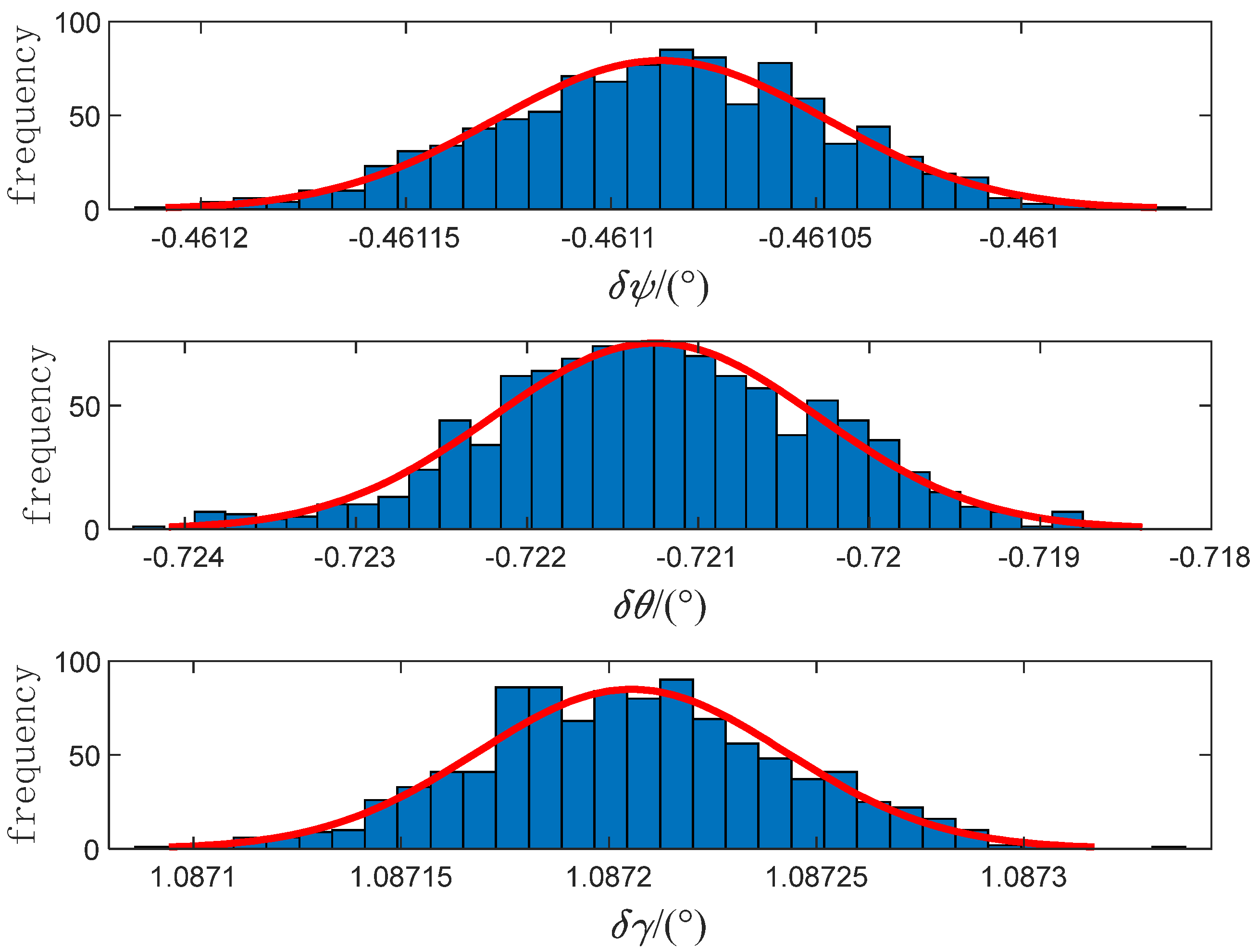
The influence of crater ellipse fitting error on OPNAV attitude determination is obtained:

$${\left({\sigma }_{}^2\right)}_f^b=C_f^{b}N{\sigma }_r{N}^{\mathrm{T}}{C}_b^f=C_f^{b}NG\left(\mathsf{\Psi }\left(X_i\right)+\mathsf{\Psi }\left(X_j\right)\right)G^{\mathrm{T}}{N}^{\mathrm{T}}{C}_b^f$$

(93)

Define the intermediate transfer matrix D:

$$D:=C_f^{b}NG$$

(94)

The influence can be expressed by $\mathsf{\Psi }\left(X\right)$ as:

$${\sigma }_C^2={\left({\sigma }_{}^2\right)}_f^b=D\left(\mathsf{\Psi }\left(X_i\right)+\mathsf{\Psi }\left(X_j\right)\right)D^{\mathrm{T}}$$

(95)

4.4. Summary of the Influence of Crater Fitting Error on OPNAV

Given the measurement error, the influence of the $\mathsf{\Psi }\left(X_i\right)$ on navigation positioning and attitude determination is:

$$\left\{\begin{array}{l}\begin{array}{cc}\mathsf{\Psi }\left(X_k\right)=C{W}_{k}MK{H}^{\mathrm{T}}{\sigma }_k^{2}H{K}^{\mathrm{T}}{M}^{\mathrm{T}}{W}_k{}^{\mathrm{T}}{C}^{\mathrm{T}}& k=i,j\end{array}\hfill \\ {\sigma }_r^2=G\left(\mathsf{\Psi }\left(X_i\right)+\mathsf{\Psi }\left(X_j\right)\right)G^{\mathrm{T}}\hfill \\ {\sigma }_C^2=D\left(\mathsf{\Psi }\left(X_i\right)+\mathsf{\Psi }\left(X_j\right)\right)D^{\mathrm{T}}\hfill \end{array}\right.$$

(96)

According to Formulas (64), (68), (77), (85), (90), (91) and (94), each intermediate matrix is as follows:

$$\left\{\begin{array}{c}\mathit{K}={\left({\mathit{H}}^{\mathrm{T}}\mathit{H}\right)}^{-1}\hfill \\ {\mathit{M}}_{2\times 5}=\frac{1}{2}{\mathit{A}}^{-1}\left[\begin{array}{cc}{\mathit{A}}^{-1}\mathit{b}& -1\end{array}\right]\left[\begin{array}{c}\delta \mathit{A}\\ \delta \mathit{b}\end{array}\right]\delta {\hat{\mathit{\Theta }}}^{\mathrm{T}}{\left(\delta \hat{\mathit{\Theta }}\delta {\hat{\mathit{\Theta }}}^{\mathrm{T}}\right)}^{-1}\hfill \\ {\mathit{W}}_{i,j}=\left[\begin{array}{ccc}{\left(Z_{i,j}^C\right)}^{-1}& 0& X_{i,j}^C{\left(Z_{i,j}^C\right)}^{-2}\\ 0& {\left(Z_{i,j}^C\right)}^{-1}& Y_j^C{\left(Z_{i,j}^C\right)}^{-2}\end{array}\right]\hfill \\ \mathit{C}=t_i^{-\frac{1}{2}}{t}_j^{-\frac{1}{2}}\left[\left.P_i^{UV}\right|P_j^{UV}\right]{\left[\begin{array}{cc}-g_{i,j}{t}_i^{-1}{\mathit{I}}_{\mathbf{2}}& {\mathit{I}}_{\mathbf{2}}\\ {\mathit{I}}_{\mathbf{2}}& -g_{i,j}{t}_j^{-1}{\mathit{I}}_{\mathbf{2}}\end{array}\right]}^{\mathrm{T}}\hfill \\ \mathit{G}=t{{}^{\prime }}_{i}t{{}^{\prime }}_j{⟮2\left(\mathit{r}-{\tilde{\mathit{P}}}_i^f-{\tilde{\mathit{P}}}_j^f\right)-{\mathit{g}}^{\prime }⟮{\left(t{{}^{\prime }}_i\right)}^{-1}+{\left(t{{}^{\prime }}_j\right)}^{-1}⟯⟯}^{-1}\hfill \\ \mathit{S}={\left({\mathit{P}}_{}^C\right)}^{\mathrm{T}}{\left({\mathit{P}}_{}^C{\left({\mathit{P}}_{}^C\right)}^{\mathrm{T}}\right)}^{-1}\hfill \\ \mathit{N}=\delta \mathit{rS}\delta {\mathit{r}}^{\mathrm{T}}{\left(\delta \mathit{r}\delta {\mathit{r}}^{\mathrm{T}}\right)}^{-1}\hfill \\ \mathit{D}={\mathit{C}}_C^b\mathit{NG}\hfill \end{array}\right.$$

(97)

Intermediate parameters in Formula (97) are:

$$\left\{\begin{array}{l}{t}_{i,j}=1+U_{i,j}^2+V_{i,j}^2\hfill \\ g_{i,j}=1+U_i{U}_j+V_i{V}_j\hfill \\ t{\prime }_{i,j}=\left|r-{\tilde{P}}_{i,j}^f\right|\hfill \\ g\prime =r^2-2\left({\tilde{P}}_i^f+{\tilde{P}}_j^f\right)r+{\tilde{P}}_i^f{\tilde{P}}_j^f\hfill \end{array}\right.$$

(98)

After detecting the crater, the existing OPNAV method usually calculates the central coordinates of the crater and directly uses this for navigation, discarding the shape, distribution, and other information of detected craters. In Formula (97), matrix K represents the distribution characteristics of craters, and matrix M represents the shape characteristics of the crater. Torus-OPNAV does not discard any information about ellipse fitting, and uses it in a high-precision inertial/optical integrated navigation system in planetary exploration.

The CDA based OPNAV algorithm proposed in this paper can work independently when more than three craters are detected. When the number of detected craters is less than 3, the OPNAV method can work normally only when it is combined with the inertial navigation system. In this case, there are two schemes for INS/OPNAV integrated navigation: (1) replace the crater feature with the crater detection vector. At this time, the optical navigation system cannot calculate the position, attitude and other information, and can only correct the inertial navigation system; (2) replace the crater feature information with the feature point information, such as ORB, and combine it with the inertial navigation system.

5. Results and Discussion

5.1. Torus-OPNAV Algorithm Feasibility Verification

Crater detection is the basis of OPNAV and hazard avoidance based on terrain characteristics. The crater database obtained in reference [8] was used as the original data. The simulation conditions are shown in

Table 1. Simulation condition of Torus-OPNAV algorithm feasibility verification.

Parameter	Value
NAVCam parameters	focal length (f)	0.008 m
	view angle($\theta$)	100°
	resolution ratio	2 m
	measurement error	~N (0, 12)
Crater parameters	Crater 1 coordinates	[−3000 2000 1] m
	Crater 2 coordinates	[−3000 3000 1] m
	Crater 3 coordinates	[1000 3000 1] m
Initial position $r_o$		[−300 50 2000] m
Time		70 s

. Torus-OPNAV algorithm was applied to optical navigation and verified.

Under the condition of observing three craters, the lander’s position was at an intersection of the 3-torus, as shown by the white dot in Figure 7. The other three intersection coordinates could be excluded because the landing orbit altitude was negative, it was below the surface of the celestial body, or the position vector direction was opposite to the actual flight direction of the lander.

Figure 8 is a partial enlarged view near the lander position, showing the intersection of three faces and the intersection of two faces. The white dot in the figure is the intersection of 3-torus, that is, the actual position of the lander.

Crater ellipse fitting and ellipse center calculation are the basis of the Torus-OPNAV method proposed in this paper. Its distribution directly affects the imaging cosine calculation, and further affects the accuracy of optical navigation position and attitude determination. According to the parameters set in Table 1, the Monte Carlo simulation experiment was carried out. The shooting times were 1000, and the length of the long and short semi axes of the crater were set to 100 m. The coordinates of the fitting ellipse center of three craters were counted and 3 σ confidence ellipses were drawn, as shown in Figure 9.

It can be seen from Figure 9 that the error of fitting ellipse center was a Gaussian distribution, and the accuracy was 1 m (3σ). On this basis, the Torus-OPNAV simulation experiment was carried out with 1000 shooting times. The simulation results are shown in Figure 10 and Figure 11. Figure 10 shows the shooting results of the Torus-OPNAV positioning accuracy simulation experiment, and Figure 11 shows the shooting results of attitude determination accuracy, including yaw angle, pitch angle, and roll angle.

5.2. Torus-OPNAV Simulation under Different Observation Conditions

In the actual lunar and Mars exploration missions, the optical navigation position and attitude determination results are also different due to the difference in the resolution and measurement error variance of the navigation camera carried by the lander, and the actual crater coordinates.

We set different measurement errors and coordinate distributions of the craters, as shown in

Table 2. Torus-OPNAV Monte Carlo simulation conditions.

Parameter	Value
NAVCam parameters	Same as Table 1.
Configuration 1	Crater 1,2,3 coordinates	Same as Table 1.
Configuration 2	Crater 1 coordinates	[3000 2000 1] m
	Crater 2 coordinates	[2000 −1000 1] m
	Crater 3 coordinates	[−1000 −3000 1] m
Measurement error	Error 1	δX0~N (0, 22) m
	Error 2	δX0~N (0, 42) m
	Error 3	δX0~N (0, 72) m
Initial position $r_o$		[−300 50 2000] m

and Figure 12. Figure 12 shows the coordinate distribution configuration of two groups of craters. Compared with configuration 1, the coordinate span of the crater in configuration 2 was larger.

Monte Carlo simulation experiments were carried out 1000 times. The experimental results are shown in

Table 3. Monte Carlo results under configuration 1 and configuration 2.

Configuration	Parameter		Error 1	Error 2	Error 3
1	Elapsed time		160.571	164.005	164.025
	Position error $(3\sigma$)/(m)	$\delta x$	2.8673	5.7877	10.3558
		$\delta y$	2.3336	4.6916	8.8206
		$\delta z$	2.4791	5.7877	9.3774
	Attitude error $(3\sigma$)/(°)	$\delta \psi$	0.4346	0.8987	1.4564
		$\delta \theta$	10.4090	24.1604	38.8603
		$\delta \gamma$	0.4163	0.8366	1.5310
2	Elapsed time		172.244	169.968	159.502
	Position error $(3\sigma$)/(m)	$\delta x$	2.2474	4.5473	7.6934
		$\delta y$	1.6995	3.6656	6.1785
		$\delta z$	0.9694	1.9780	3.4999
	Attitude error $(3\sigma$)/(°)	$\delta \psi$	3.1565	6.5668	11.9348
		$\delta \theta$	5.8700	12.6747	21.7557
		$\delta \gamma$	2.7599	5.9758	9.8372

. By analyzing Table 3, the following conclusions can be drawn:

(1) No matter what kind of crater distribution configuration was selected and what kind of measurement error variance was set, the running time of the Torus-OPNAV algorithm was almost the same, and the real-time performance was good. The position and attitude determination of optical navigation could be completed within 180 ms;

(2) The accuracy of the Torus-OPNAV position and attitude determination was affected by the geometrical configurations of the crater. With the same measurement error variance, the larger the coordinate span of the craters, the better the position and attitude determination results;

(3) The celestial (z-direction) position accuracy of the lander was higher because the imaging cosine was more sensitive to the height of the lander.

During the descent and landing of the lander, due to the influence of errors such as the chattering of the lander, attitude change, and image distortion, when the image with a resolution of 1 m/pixel was detected, and the measurement error was better than $\mathcal{N}\left(0,2^2\right)$, according to the simulation results in Table 3, the Torus-OPNAV position determination accuracy, based on the spatial position distribution model, could reach the meter level, and the attitude determination was better than 7° (3σ).

5.3. Hardware-in-the-Loop Simulation

To verify the reliability of the proposed Torus-OPNAV algorithm, a hardware-in-the-loop simulation test was carried out. The test verification system was composed of a lunar sand table, UAV (unmanned aerial vehicle)-equivalent flight platform, indoor optical tracking system (OptiTrack, Corvallis, OR, USA), etc., as shown in Figure 13.

The parameters of the sand table, NAVCam, and other test equipment are as shown in

Table 4. Hardware parameters.

Hardware	Parameter
PC	CPU	Intel i9-10900
	RAM	32 G
Lunar sand table	Size	2 m × 2 m
	Maximum depth of crater	0.30 m
	Reference height of sand table	0.18 m
Light source	Color temperature	5600 K × 2
Optical tracking system	Accuracy	0.01 m
NAVCam	45fps@1280 × 60, 60fps@1280 × 720 80fps@640 × 480, 160fps@320 × 240

. We made the UAV hover over the lunar sand table, took real-time photos of the table, extracted the craters, and calculated the attitude and position of the UAV. Then, we compared the calculation results with the reference truth value provided by OptiTrack to verify the accuracy and reliability of the algorithm. Three craters in the field of view were randomly selected for navigation in each test.

Comparing the Torus-OPNAV proposed in this paper with the OPNAV method, based on the gradient descent (GD) method and improved gradient descent (IGD) method, we calculated the RMSE value of the position and attitude determination accuracy of the three methods, and compared their running time. The number of target practice was 1000, and the simulation results are shown in the Figure 14, Figure 15 and Figure 16.

The accuracy of the three methods was basically the same. The Torus-OPNAV algorithm was obviously superior to the traditional OPNAV based on the GD method and the IGD method in terms of time consumption.

6. Conclusions

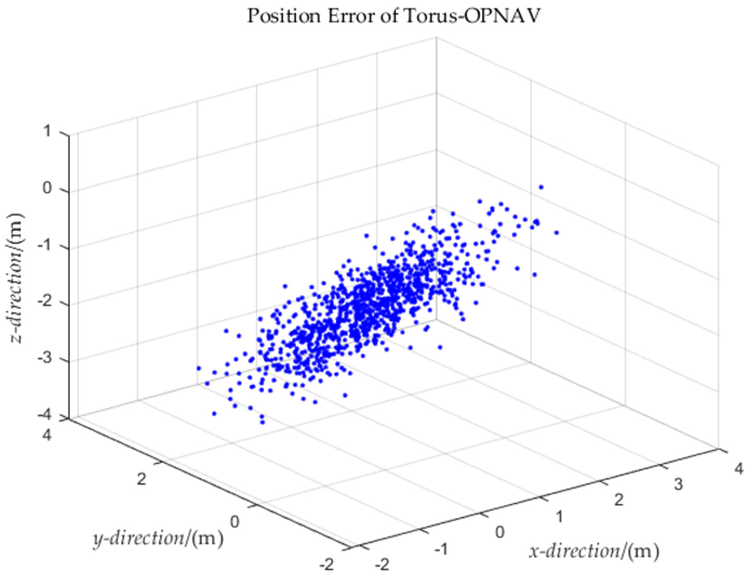
In this paper, an optical navigation method based on a spatial position distribution model was proposed to solve the problem of high-precision optical navigation for the descent and landing of lunar and planetary landers. According to the correspondence of objects and images between two craters and the cosine of imaging, the spatial position distribution of the lander relative to the two craters was calculated and described as a self-intersecting spatial torus of the Abelian Lie group. Using this characteristic, when more than two craters were observed, the high-efficiency, high-precision optical navigation of the landing lander could be realized by analyzing the intersecting relationship between the lander and the torus. The crater detection error and its influence on optical imaging and optical navigation were analyzed, and the theoretical accuracy of the optical navigation system based on the crater detection algorithm was demonstrated.

Theoretical analysis and simulation experiments showed that, compared with the traditional optical navigation method based on crater detection, the proposed method had the following advantages: (1) After the crater was detected and imaged, the imaging mathematical relationship was further analyzed and discussed. The relationship between the optical imaging information and the spatial position distribution of the lander was revealed. It was demonstrated that the spatial distribution surface of the position was a torus, which was described by a set of parameter formulas. On this basis, the mathematical relationship between positioning and attitude determination of optical navigation system could be decoupled, and the amount of calculation of optical navigation could be reduced. (2) From crater detection to optical navigation, it was difficult to accurately match the center and shape of the detected crater with the true value, due to measurement errors. In this paper, the error propagation characteristics of the detection error in the process of least squares fitting, imaging cosine calculation, and nonlinear iteration were derived in detail. The imaging cosine variance contribution function was proposed to analyze the influence of Crater Observation Error on optical navigation positioning and attitude determination. (3) The imaging cosine variance contribution function could be directly used to adjust the error variance matrix R in the filter, making the optical navigation system adaptive to the current environment and improved the navigation accuracy. (4) The proposed algorithm could directly calculate the absolute position information of the lander on the basis of detecting craters and other features. The positioning accuracy (especially the celestial positioning accuracy) was high and the real-time performance was good.