Nonlinear Dynamic Modeling of Joints between Solar Panels on Spacecraft

Abstract

Multiple linear and nonlinear dynamic parameters of the joints at the root of solar panels and between solar panels on spacecraft, both of which have complex nonlinear dynamic properties, were identified by using the force state mapping method for modeling complex nonlinear joints in deployable mechanisms of spacecraft, and the differential equations representing the nonlinear dynamic model of the joints were derived. On the basis of the actual force characteristics of the joints, test systems were developed to investigate the vibration response of the complex nonlinear joints in spacecraft so as to acquire test data necessary for the identification. The relation between the moment and bending angle of the panel root and inter-panel joints on spacecraft was obtained through vibration tests under various frequencies and excitation forces. The validity and effectiveness of the dynamic model have been verified by vibration tests of the joints under pulsed excitation. The parameters identified in this paper reflect the nonlinear stiffness, friction and damping characteristics of the joints. The dynamic model established based on these parameters can describe multiple linear and nonlinear dynamic properties of the joints and can be further applied in modeling and control of the entire spacecraft system.

1. Introduction

Hinge joints are used between solar panels, antennae, and other accessories of spacecraft to carry out folding and on-orbit unfolding. The joints on spacecraft are complex in structure and consist of many components with clearance between them. Under external load, collision and friction would occur between the components, thus resulting in obviously nonlinear stiffness and damping characteristics of the joints, which make it very complex and difficult to determine the joints’ dynamic parameters and establish models for them. Dynamic experiments on existing spacecraft structures have shown that joints are the main source of nonlinearity of deployable mechanisms on spacecraft [1]. Therefore, it is important to analyze and test the dynamic characteristics of the joints and develop accurate dynamic models for the dynamic modeling of deployable mechanisms on spacecraft.

Dynamic characteristics of the joints have been studied by numerous scholars both in China and abroad to develop dynamic models. Ren [2] assumed that the difference in dynamic characteristics between the joint and joint assembly is due to the influence of the joint and extracted dynamic parameters of the joint from frequency response functions of the structures. Wang et al. [3] estimated all the unmeasured frequency response functions of the joint based on measured frequency response functions and identified linear dynamic characteristics of the joint in the assembly based on both the measured and estimated frequency response functions. However, only linear dynamic characteristics of the joint were taken into account in the above studies with the influence of nonlinear factors being neglected. Hence, there would be some difference between the actual structure and the joint model established by using the above methods.

Boswald [4] proposed a method of identifying parameters of nonlinear joints by use of frequency response residuals. In this method, the difference between nonlinear frequency response function values obtained through analysis and tests, respectively, is used to renew linear and nonlinear parameters in the finite element model of the joint, so as to improve the ability of the finite element method to describe the dynamic behavior of nonlinear joints. System identification is an important method for developing dynamic models of complex structures. A lot of nonlinear dynamic system identification methods based on time domain or frequency domain have been developed [5,6,7]. Among them, the force state mapping method proposed by Crawley [8,9] is an important time-domain nonlinear system identification method, which expresses a structure’s restoring force as a single-valued surface of displacement and velocity in a 3D space, and its profile reflects the structure’s linear and nonlinear characteristics. Kim [10] then proposed a frequency domain force state mapping method. Masters [11] applied the force state mapping method in parameter identification of multi-DOF frame structures. Meskell et al. [12] applied the force state mapping method in the elastic fluid system and identified linear and nonlinear stiffness and damping parameters of the system. Namdeo [13] used the reproducing kernel particle method and the Kriging method to fit force state maps, and this method is applicable for multi-DOF non-smooth nonlinear systems. Although scholars have carried out studies on dynamic characteristics of nonlinear joints, they only acquired part of the nonlinear parameters of the joints [14,15,16,17]. Up to now, no study on comprehensive dynamic parameter identification and modeling of nonlinear joints on spacecraft has been reported.

Vibration response parameters of the joints at the root of solar panels (panel root joint) and between solar panels (inter-panel joint) on spacecraft were obtained through dynamic tests under different excitation frequencies and a nonlinear dynamic model was established for the two joint structures by using the force state mapping method. The testing program was designed according to the force characteristics of the complex nonlinear joints on spacecraft, and test systems were developed to investigate the vibration response of the joints in spacecraft so as to obtain the relation between moment and bending angle of the joints under various frequencies and excitation forces. Based on the test data, the force state mapping method was used to perform nonlinear dynamic parameter identification for the two types of joints, respectively, and their nonlinear stiffness, friction, and damping parameters were acquired. Then, the dynamic model representing nonlinear characteristics of the joints was established based on the identification results. Finally, vibration tests of the joints were conducted under pulsed excitation, and the validity and effectiveness of the dynamic model have been verified by comparing the test results with simulated results of the model.

2. Dynamic Characteristics of the Joints

The panel root and inter-panel joints are two commonly used joint structures on spacecraft, connecting the main body of the spacecraft with solar panels as well as two adjacent solar panels. At the launch of the spacecraft, the jointed solar panels are folded in the carrier. After injection, they are unfolded to working condition with the joints locked. At this time, the solar panels would be subject to violent vibration when disturbed, due to their large size, low stiffness, and high flexibility, and the vibration would be obviously nonlinear due to the nonlinearity of the joints. Therefore, the premise behind vibration control of the solar panels is to analyze the dynamic characteristics of the joints and determine their dynamic parameters at this condition. This paper is mainly concerned with the dynamic characteristics of the panel root and inter-panel joints on spacecraft in a locked-in state. Because most of the solar panels are rectangular with small transverse bending stiffness, their bending vibration in response to external disturbance is mainly first-order transverse bending vibration under certain conditions and the bending moment is mainly borne by the panel root and inter-panel joints. So, they can be approximate to single-degree-of-freedom nonlinear structures.

3. Dynamic Experiments for the Joints

3.1. Experimental Equipment and Program

According to the structures of the panel root and inter-panel joints and their force characteristics in the system, test systems were designed to investigate their vibration response and dynamic experiments were carried out to acquire test data necessary for the system identification.

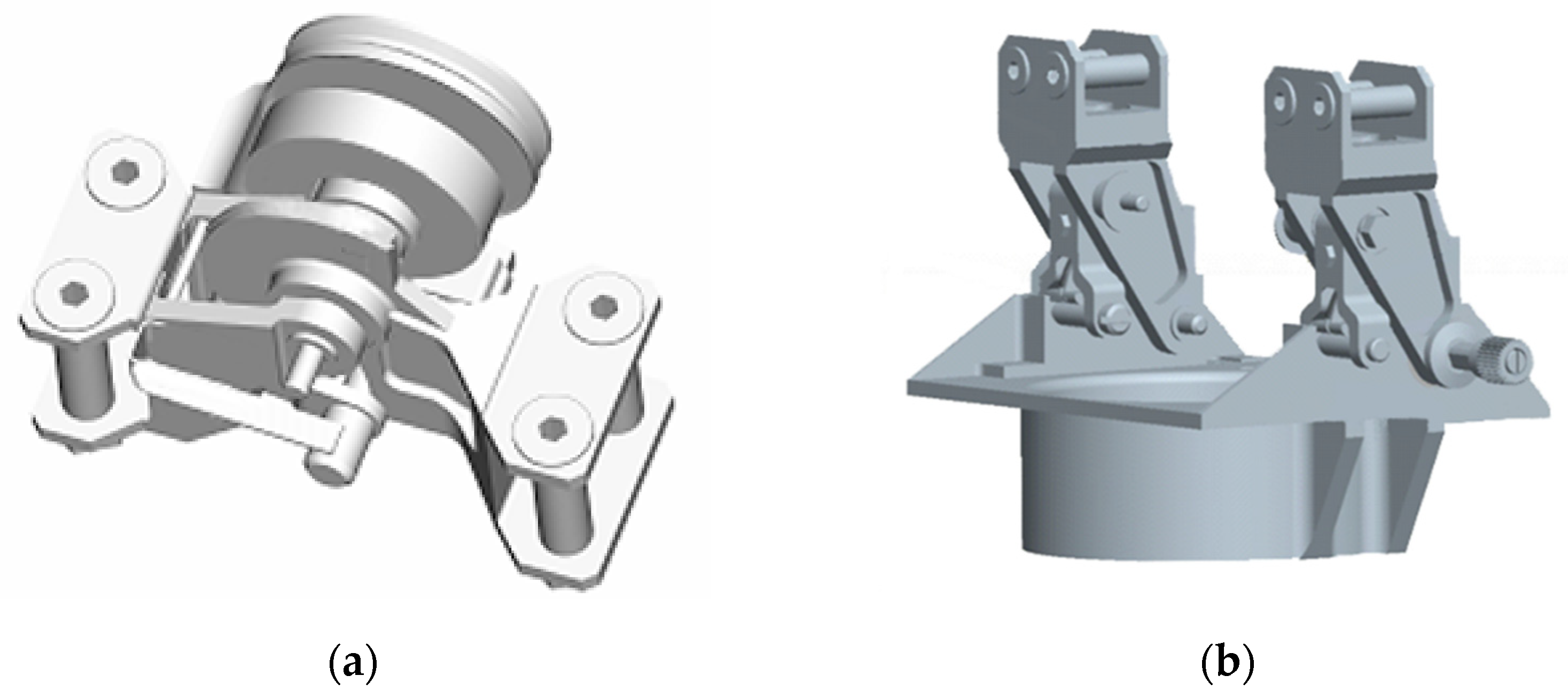
The experimental subjects were inter-panel and panel root joints on the solar panels of spacecraft, as shown in Figure 1. Single-frequency excitations were used in the experiments. The solar panels on spacecraft possess low stiffness when they are unfolded on-orbit in space [18,19]. Because inherent frequency of the solar panels with these joints is intensively located between 3 Hz and 6 Hz, 3 Hz, 4 Hz, 5 Hz, and 6 Hz single-frequency signals were used as excitation signals in the vibration tests for the joints.

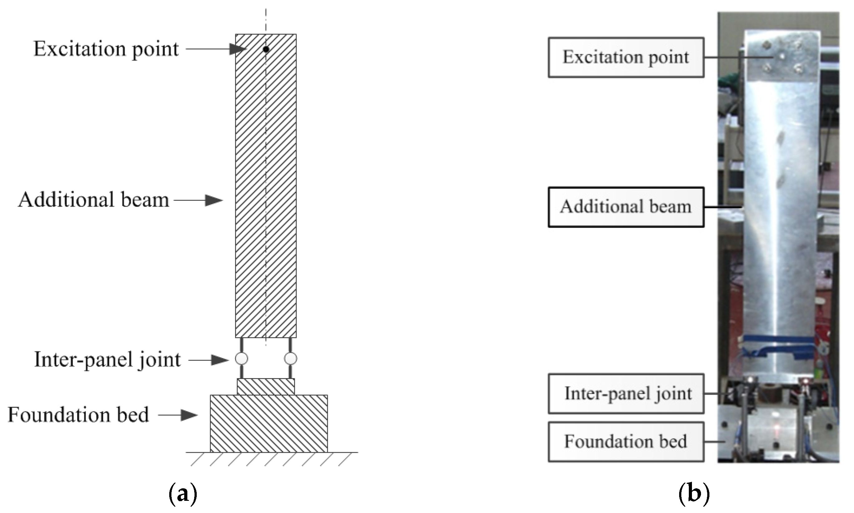
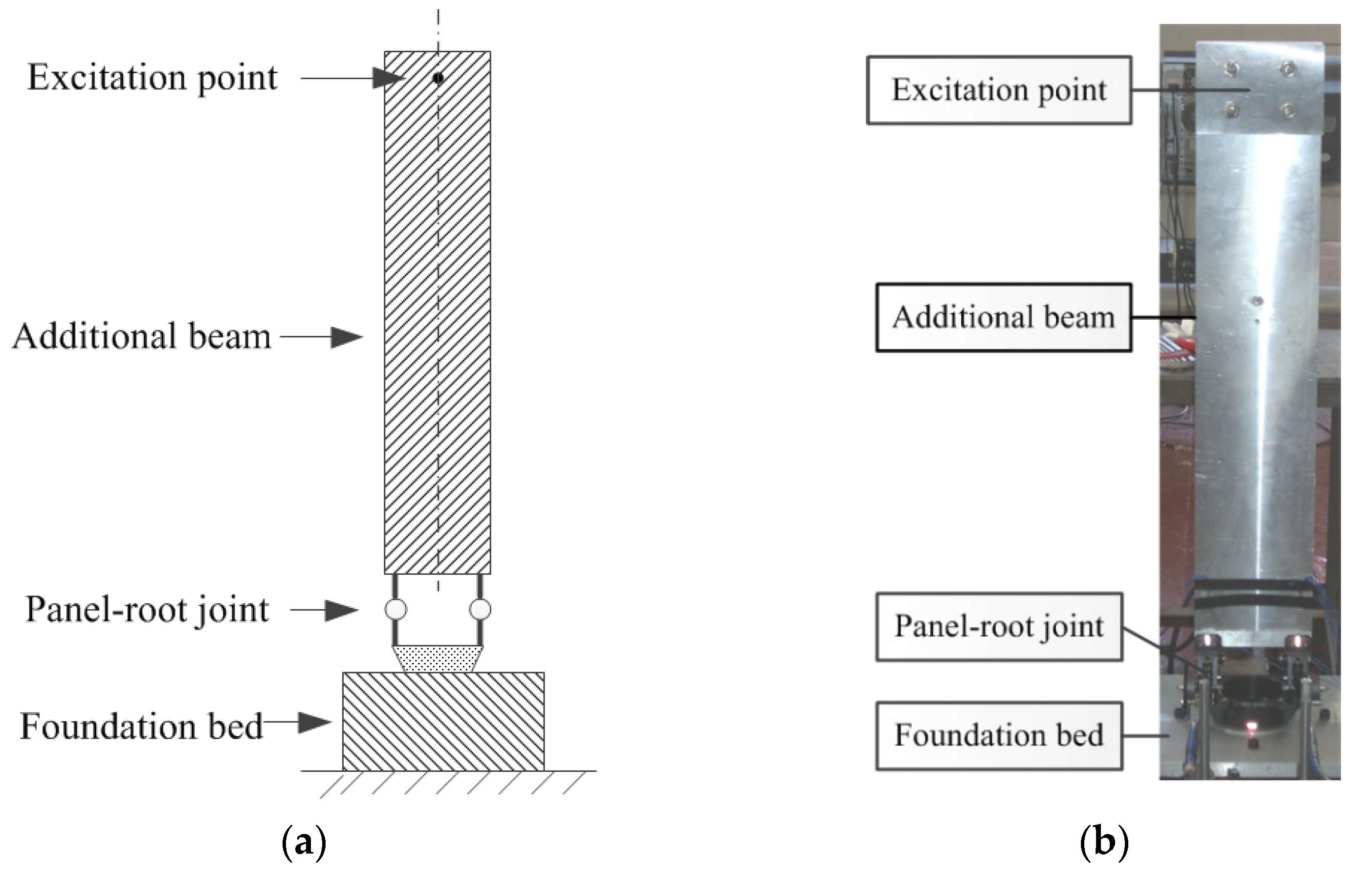
Because the inter-panel joint is similar to the panel root joint in structure, the experimental programs for them were similar as well. Physical parameters that were obtained in the experiments included dynamic moment at the end of the joints and their dynamic bending angle. For the convenience of force application and parameter measurement, an additional beam was connected at one end of the joints, and the other end was fixed on the test bed. In addition, the vertical installation was used to ease the installation of experimental equipment and the implementation of the experiments. Figure 2 and Figure 3 show the schematic diagram and photograph of the experimental facility. The electromagnetic excitation system, consisting of a power amplifier and an exciter fixed at the bottom, was used to apply excitation force on the joints. The excitation force produced by the exciter was applied to the excitation point at the end of the beam through a straight bar. Dynamic strain at the junction of the additional beam and the joint was measured by using a strain gauge and a dynamic strain gauge, and dynamic displacement at the end of the joint was measured by using a non-contact laser vibrometer. 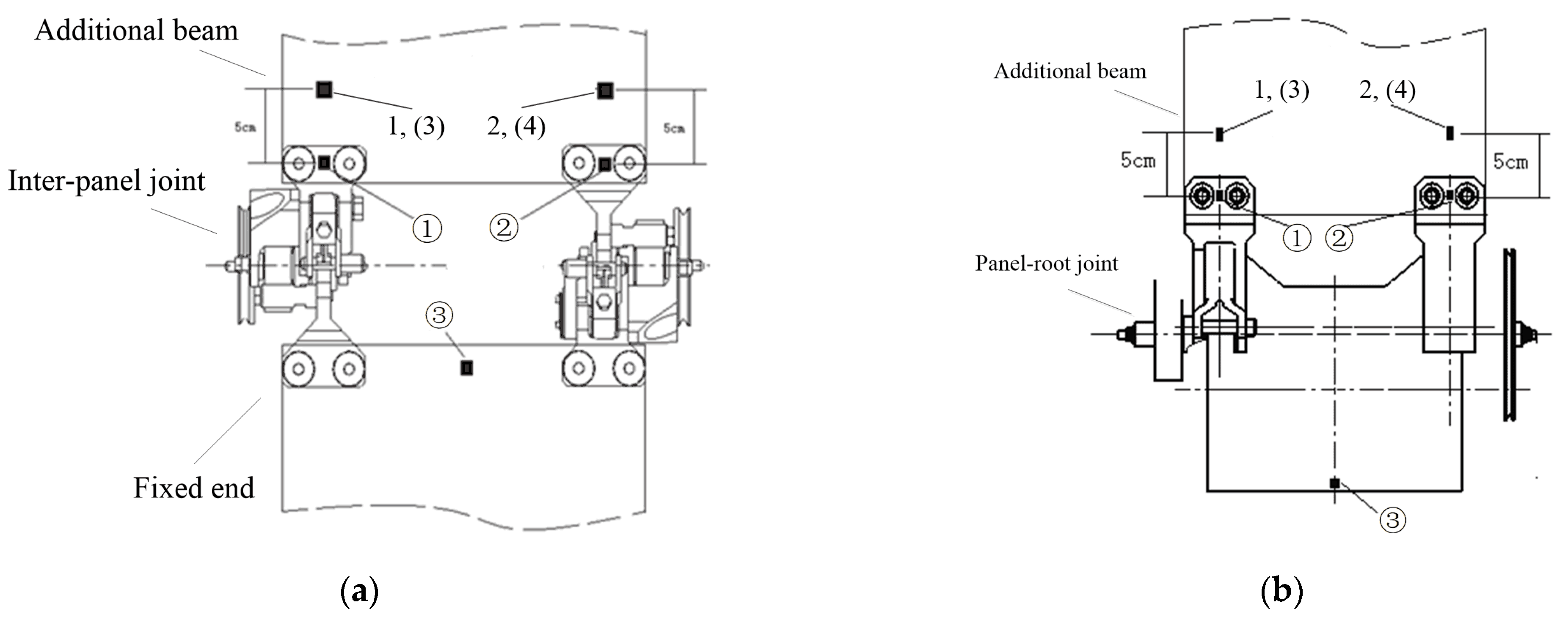Figure 4 shows the arrangement of measurement points for strain and displacement on the inter-panel and panel root joints. Where the measurement points for strains 1, 2, 3, and 4 are arranged at the bottom of the beam; the measurement points for displacement ①, ②, and ③ are arranged at the top and bottom of the joint.

Under the control of control signals, the exciter output excitation force at a certain frequency, driving the additional beam to move and applying a dynamic moment on the joint that was connected at the lower end of the beam. At certain sampling time and sampling frequency, dynamic strain values were obtained at the strain measurement point located at the lower end of the beam through the strain gauges and dynamic strain gauge, and the dynamic bending moment at this point on the section of the beam can be thus calculated. The dynamic bending moment was approximately equal to the dynamic moment on the upper end of the joint. Displacement at the upper and lower ends of the joints was obtained through the laser vibrometer, and the dynamic bending angle corresponding to the dynamic distortion of the joint under the above dynamic moment can be calculated. The time history of the dynamic strain and displacement was recorded through the data acquisition and processing system.

3.2. Experimental Results

The dynamic moment and dynamic bending angle under the action of a certain excitation force can be calculated based on the measured data in the above dynamic experiments on the inter-panel and panel root joints. Considering that the full-bridge mode was used when using the dynamic strain gauge to measure the strain data, the strain at the lower end of the additional beam can be written as:

$$\mathit{\epsilon }(t)=\frac{{\mathit{\epsilon }}_1(t)+{\mathit{\epsilon }}_2(t)-{\mathit{\epsilon }}_3(t)-{\mathit{\epsilon }}_4(t)}{4}$$

(1)

where ${\mathit{\epsilon }}_1(t)$, ${\mathit{\epsilon }}_2(t)$, ${\mathit{\epsilon }}_3(t)$, and ${\mathit{\epsilon }}_4(t)$ are the strain values, respectively, measured at the measurement points 1, 2, 3, and 4 at the same time. ${\mathit{\epsilon }}_3(t)$ and ${\mathit{\epsilon }}_4(t)$ have the opposite sign to ${\mathit{\epsilon }}_1(t)$ and ${\mathit{\epsilon }}_2(t)$ due to points 3 and 4 at the opposite side of the beam as points 1 and 2.

The moment on the upper end of the joints was approximately equal to the bending moment on the section of the beam at its lower end, which can be calculated as follows:

$$\mathit{M}(t)=\beta \frac{2E{I}_{\mathrm{z}}\mathit{\epsilon }(t)}{h}$$

(2)

where $E{I}_{\mathrm{z}}$ is the bending stiffness of the additional beam; $h$ is the height of the beam section; $\beta$ is the position correction factor of the strain gauges, which is related to the actual places of the strain gauges.

The bending angle of the joint can be calculated through the following equation:

$$\mathit{\theta }(t)\approx \frac{\left({\mathit{d}}_1(t)+{\mathit{d}}_2(t)\right)/2-{\mathit{d}}_3(t)}{L}$$

(3)

where ${\mathit{d}}_1(t)$, ${\mathit{d}}_2(t)$, and ${\mathit{d}}_3(t)$ are the displacement values, respectively, measured at the measurement points ①, ②, and ③ at the same time; $L$ is the length of the joint.

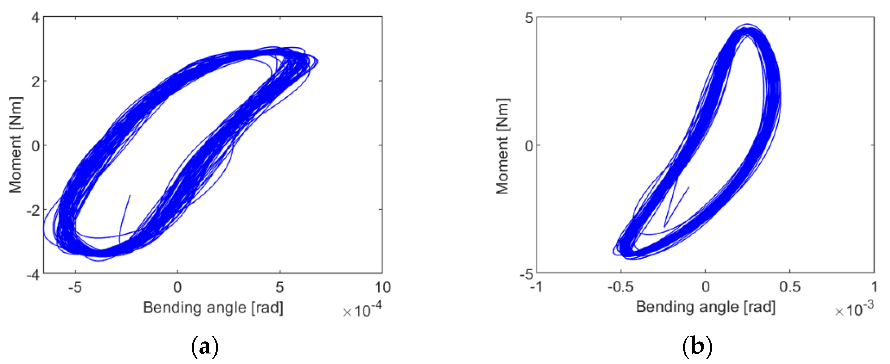
Figure 5 shows the moment bending angle curves of the inter-panel and panel root joints at the excitation frequency of 3 Hz, which were plotted after filtering and removing high-frequency noise from the acquired data. The moment bending angle hysteresis loop, shown in Figure 5, fully reflects the complex nonlinearity of the stiffness and damping of the two joint structures.

4. Dynamic Modeling of the Joints

4.1. Force State Mapping Method

For a nonlinear system, its state can be described solely by displacement $\mathit{x}$ and velocity $\dot{\mathit{x}}$, and the dynamic model of the system can be expressed as a second-order nonlinear differential equation:

$$\mathit{M}\ddot{\mathit{x}}+\mathit{C}\left(\mathit{x},\dot{\mathit{x}}\right)\dot{\mathit{x}}+\mathit{K}\left(\mathit{x},\dot{\mathit{x}}\right)\mathit{x}=\mathit{F}(t)$$

(4)

where the generalized damping $\mathit{C}$ and generalized stiffness $\mathit{K}$ are functions of system state.

Equation (4) can be transformed to:

$${\mathit{F}}_{\mathrm{T}}\left(\mathit{x},\dot{\mathit{x}}\right)=\mathit{C}\left(\mathit{x},\dot{\mathit{x}}\right)\dot{\mathit{x}}+\mathit{K}\left(\mathit{x},\dot{\mathit{x}}\right)\mathit{x}=\mathit{F}\left(t\right)-\mathit{M}\ddot{\mathit{x}}$$

(5)

where ${\mathit{F}}_{\mathrm{T}}$ is the overall transfer force of the system, expressed as a function of instantaneous system state and called transfer force.

A 3D curved surface describing the transfer force of the system ${\mathit{F}}_{\mathrm{T}}$ and its corresponding state $\left(\mathit{x},\dot{\mathit{x}}\right)$ can be obtained through Equation (5), and it is called a force state map, which reflects the relation between the transfer force ${\mathit{F}}_{\mathrm{T}}$, displacement $\mathit{x}$, and velocity $\dot{\mathit{x}}$. Dynamic parameters of the system can be obtained. Displacement, velocity, accelerated velocity, and external force of the system at each time period need to be known for making the force state map. 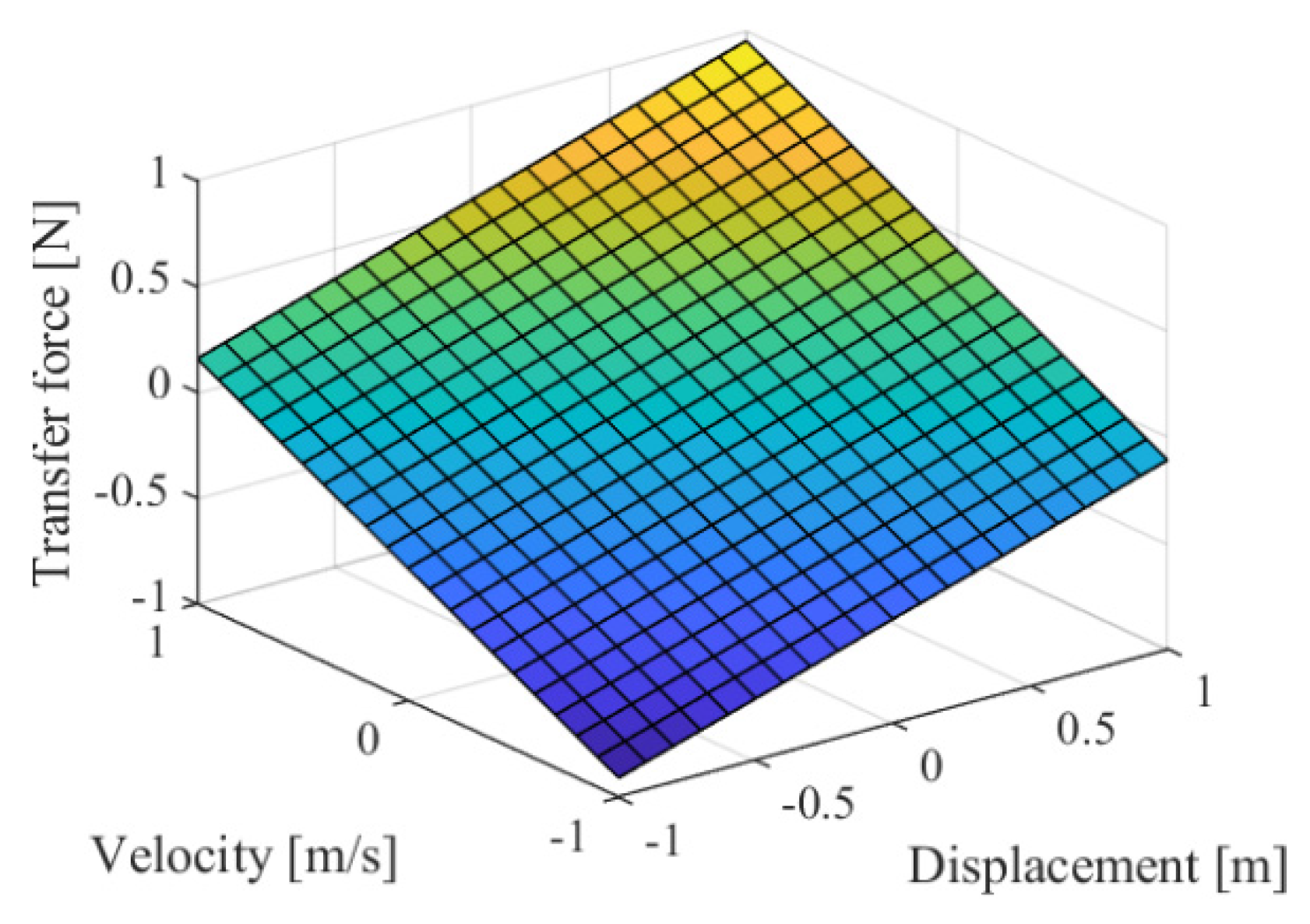Figure 6 shows the force state map of a linear spring mass damper system, which is an oblique plane. The slope of transfer force to displacement is the linear stiffness of the system $k$, and the slope to velocity is the linear damping of the system $c$.

According to the above theory, the general steps of system identification by use of the force state mapping method are as follows: first, apply a certain dynamic force on the system, and measure the state of the system under the action of the force at the meantime; then, process the measured data and draw the force state map; at last, extract relevant dynamic parameters from the map and establish a dynamic model for the system.

4.2. Dynamic Modeling

Through the dynamic experiments described in Section 3, the moment and corresponding bending angle of the inter-panel and panel root joints at the four excitation frequencies were obtained. Corresponding angular velocity and angular acceleration can be calculated through numerical differentiation of the bending angle after filtering for the data. Then, the transfer moment ${\mathit{M}}_{\mathrm{T}}$ and corresponding state $\left(\mathit{\theta },\dot{\mathit{\theta }}\right)$ can be obtained.

Because the transfer moment exhibits a spiral rotation in the state space, the 3D curved surface describing the relation between the transfer moment ${\mathit{M}}_{\mathrm{T}}$ and the corresponding bending angle $\mathit{\theta }$ and angular velocity $\dot{\mathit{\theta }}$ cannot be directly plotted. For this reason, the intervals of bending angle and angular velocity can be divided into $n$ subintervals, and $n\times n$ subdomains can be thus obtained through permutation and combination. The 3D force state curved surface of the transfer moment ${\mathit{M}}_{\mathrm{T}}^{\prime }(i)$ and corresponding state subdomain can be then plotted by averaging all the transfer moments ${\mathit{M}}_{\mathrm{T}}^{\prime }(i)$ ($i=1,2,\cdots ,n\times n$) corresponding to the subdomains. 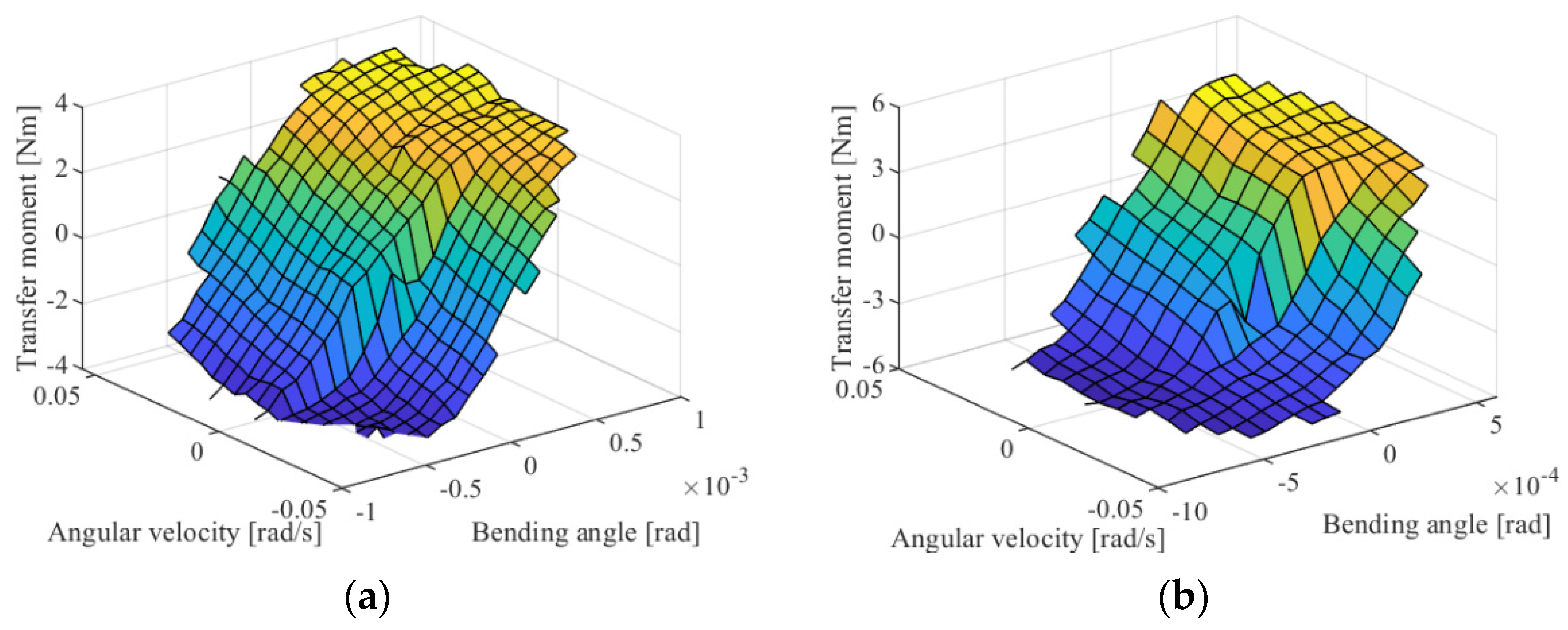Figure 7 shows the force state map of the inter-panel and panel root joints at the excitation frequency of 3 Hz.

As can be seen from Figure 7, the two types of joints have similar force state maps, both exhibiting highly nonlinearity and similar dynamic characteristics. When the angular velocity is 0, the transfer moment of them shows a step change, indicating that Coulomb friction exists in the two structures. Meanwhile, the transfer moment and angular velocity have a linear relation, indicating that linear viscous damping exists in the structures. For the same angular velocity, the transfer moment of the two types of joints changes nonlinearly with the bending angle, which means there is a nonlinear elastic force in the structures and the structures can be described jointly by a linear spring, a quadratic nonlinear spring, and a cubic nonlinear spring. Based on the above analysis and Reference [9], the transfer moment of the two types of joints can be written as:

$${\mathit{M}}_{\mathrm{T}}=\left[c_1\hspace{0.17em}\hspace{0.17em}{k}_1\hspace{0.17em}\hspace{0.17em}{k}_2\hspace{0.17em}\hspace{0.17em}{k}_3\hspace{0.17em}\hspace{0.17em}{M}_F\right]\left[\begin{array}{c}\dot{\mathit{\theta }}\\ \mathit{\theta }\\ {\mathit{\theta }}^2\\ {\mathit{\theta }}^3\\ \mathrm{sign}\left(\dot{\mathit{\theta }}\right)\end{array}\right]=c_1\dot{\mathit{\theta }}+k_1\mathit{\theta }+k_2{\mathit{\theta }}^2+k_3{\mathit{\theta }}^3+M_F\mathrm{sign}\left(\dot{\mathit{\theta }}\right)$$

(6)

where the first term on the right side of the equation is the linear damping moment; $c_1$ is the linear damping coefficient; the second term is the linear elastic moment; $k_1$ is the stiffness coefficient of the linear spring; the third and fourth terms are the nonlinear elastic moment; $k_2$ and $k_3$ are the stiffness coefficients of the nonlinear springs; the fifth term is the Coulomb friction moment; $M_F$ is the Coulomb friction factor. Dynamic equations of the two types of joints can be obtained by transforming Equation (6):

$$\left[I\hspace{0.17em}\hspace{0.17em}{c}_1\hspace{0.17em}\hspace{0.17em}{k}_1\hspace{0.17em}\hspace{0.17em}{k}_2\hspace{0.17em}\hspace{0.17em}{k}_3\hspace{0.17em}\hspace{0.17em}{M}_F\right]\left[\begin{array}{c}\ddot{\mathit{\theta }}\\ \dot{\mathit{\theta }}\\ \mathit{\theta }\\ {\mathit{\theta }}^2\\ {\mathit{\theta }}^3\\ \mathrm{sign}\left(\dot{\mathit{\theta }}\right)\end{array}\right]=I\ddot{\mathit{\theta }}+c_1\dot{\mathit{\theta }}+k_1\mathit{\theta }+k_2{\mathit{\theta }}^2+k_3{\mathit{\theta }}^3+M_F\mathrm{sign}\left(\dot{\mathit{\theta }}\right)=\mathit{M}$$

(7)

The least square method was used to perform the surface fitting for the force state maps of the inter-panel and panel root joints, shown in Figure 8, so as to determine the parameters in the dynamic equations for the two types of joints. The fitting was performed by using bending angle and angular velocity as independent variables, and a binary cubic polynomial as the fitting function. The RMS errors are 0.494 N∙m and 0.787 N∙m, respectively, and the coefficients of the polynomial are dynamic parameters of the two types of joints. Following the above procedure, parameter identification was then performed for the test data of the two types of joints acquired at the excitation frequencies of 4 Hz, 5 Hz, and 6 Hz, respectively.

Table 1. Results of parameter identification for the inter-panel joint.

Excitation Frequency [Hz]	k1 [N·m/rad]	k2 [N·m/rad2]	k3 [N·m/rad3]	c1 [N·m·s/rad]	${\mathit{M}}_{\mathit{F}}[\mathbf{N}·\mathbf{m}]$
3	$6.153\times {10}^3$	$-2.209\times {10}^5$	$-2.761\times {10}^9$	$4.668\times {10}^1$	$1.892\times {10}^0$
4	$6.134\times {10}^3$	$-1.625\times {10}^5$	$-2.733\times {10}^9$	$4.900\times {10}^1$	$1.821\times {10}^0$
5	$5.912\times {10}^3$	$-1.901\times {10}^5$	$-2.739\times {10}^9$	$4.851\times {10}^1$	$1.840\times {10}^0$
6	$6.063\times {10}^3$	$-1.972\times {10}^5$	$-2.501\times {10}^9$	$4.832\times {10}^1$	$1.916\times {10}^0$
Average value	$6.066\times {10}^3$	$-1.927\times {10}^5$	$-2.684\times {10}^9$	$4.813\times {10}^1$	$1.867\times {10}^0$
Standard deviation	$9.476\times {10}^1$	$2.082\times {10}^4$	$1.059\times {10}^8$	$8.651\times {10}^{-1}$	$3.831\times {10}^{-2}$

and

Table 2. Results of parameter identification for the panel root joint.

Excitation Frequency [Hz]	k1 [N·m/rad]	k2 [N·m/rad2]	k3 [N·m/rad3]	c1 [N·m·s/rad]	${\mathit{M}}_{\mathit{F}}[\mathbf{N}·\mathbf{m}]$
3	$1.060\times {10}^4$	$-6.601\times {10}^5$	$-7.741\times {10}^9$	$5.468\times {10}^1$	$2.110\times {10}^0$
4	$1.231\times {10}^4$	$-5.988\times {10}^5$	$-7.366\times {10}^9$	$5.401\times {10}^1$	$2.145\times {10}^0$
5	$1.279\times {10}^4$	$-6.304\times {10}^5$	$-7.310\times {10}^9$	$5.432\times {10}^1$	$2.128\times {10}^0$
6	$1.115\times {10}^4$	$-6.200\times {10}^5$	$-7.282\times {10}^9$	$5.329\times {10}^1$	$2.379\times {10}^0$
Average value	$1.171\times {10}^4$	$-6.273\times {10}^5$	$-7.425\times {10}^9$	$5.407\times {10}^1$	$2.191\times {10}^0$
Standard deviation	$8.764\times {10}^2$	$2.208\times {10}^4$	$1.851\times {10}^8$	$5.115\times {10}^{-1}$	$1.095\times {10}^{-1}$

show the results of parameter identification for the inter-panel and panel root joints, respectively.

As can be seen from Table 1 and Table 2, standard deviations of the identified parameters of the two types of joints are relatively small in the frequency range of 3–6 Hz, and the parameters show no obvious trends of changing with the frequency, indicating that the parameters are basically unaffected by the frequency. Therefore, the dynamic equations of the two types of joints can be obtained by substituting the averages in Equation (7). Moreover, the parameter values of the panel root joint are all larger than that of the inter-panel joint, which indicates that the panel root joint has higher stiffness, damping, and friction than the inter-panel joint.

5. Experimental Verification and Analysis

The structure connecting the joint with the beam was designed to verify the validity of the dynamic equations, and the results of the vibration response experiments were compared with the simulated results. Because the inter-panel and panel root joints are similar in both structure and dynamic characteristics, only one joint structure, the inter-panel joint in this paper, was selected for the verification of its dynamic equation. A system consisting of two beam segments that were connected by an inter-panel joint was designed to simulate the connection between the joint and actual solar panels. Pulsed excitation forces were applied to the system and the system’s responses were measured.

5.1. Experiments

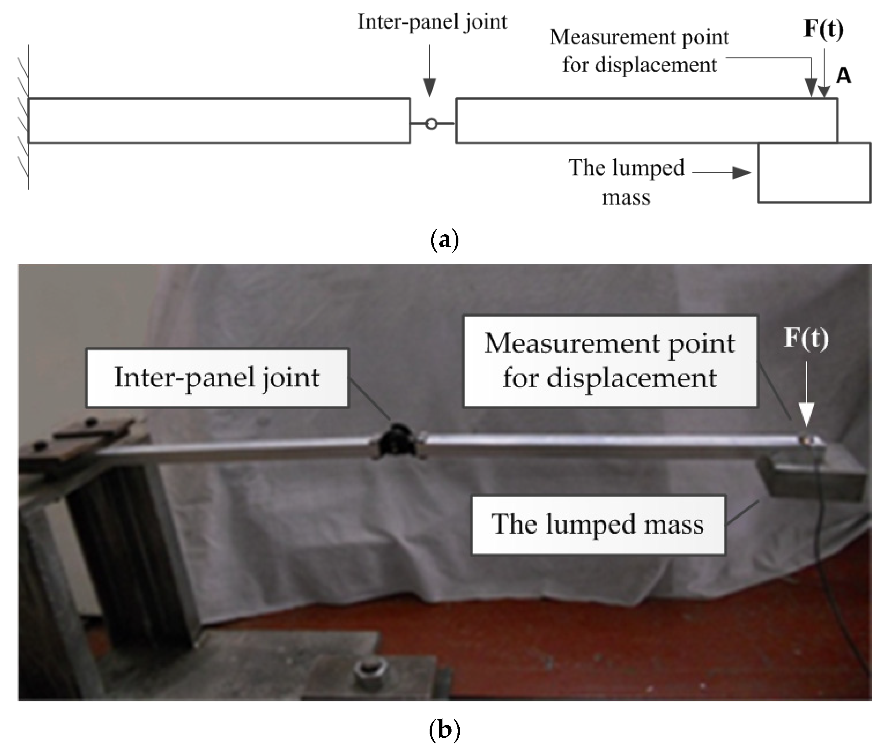
Figure 8 shows the schematic diagram and photograph of the experimental system, consisting of an inter-panel joint, two identical beam segments that were connected by the joint, and a lumped mass. The inter-panel joint was of the same type as that used in the dynamic experiments. One end of the system was fixed, while the other end was free. The lumped mass was attached to the free end. Considering the impact of the lumped mass, the horizontal installation was employed for the system to ease the implementation of the experiments. An exciting hammer was used as the force application device, and a non-contact laser vibrometer was used to measure the displacement. 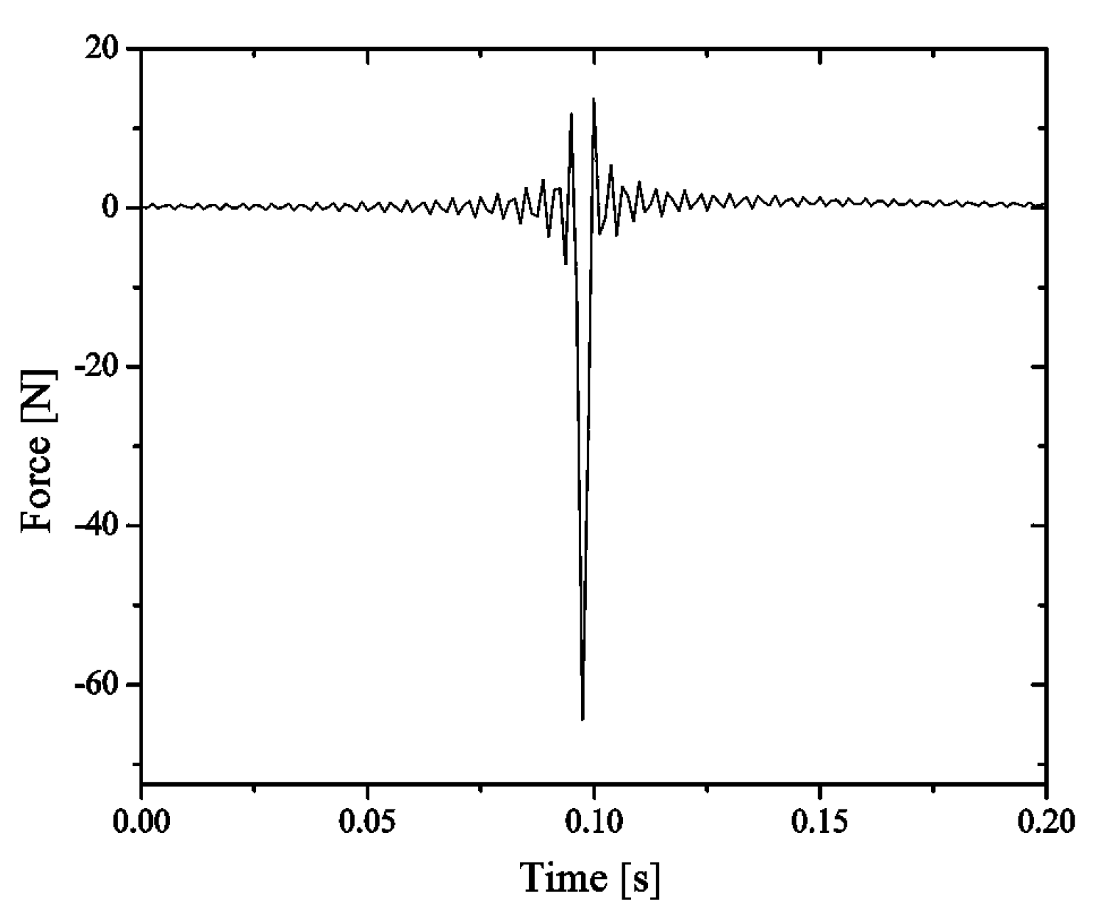In the experiment, a hammer exciting force $\mathit{F}\left(t\right)$ was applied at Point A at the free end of the system, and the displacement response at this point was measured. The time history of the force and displacement was recorded through the data acquisition and processing system.

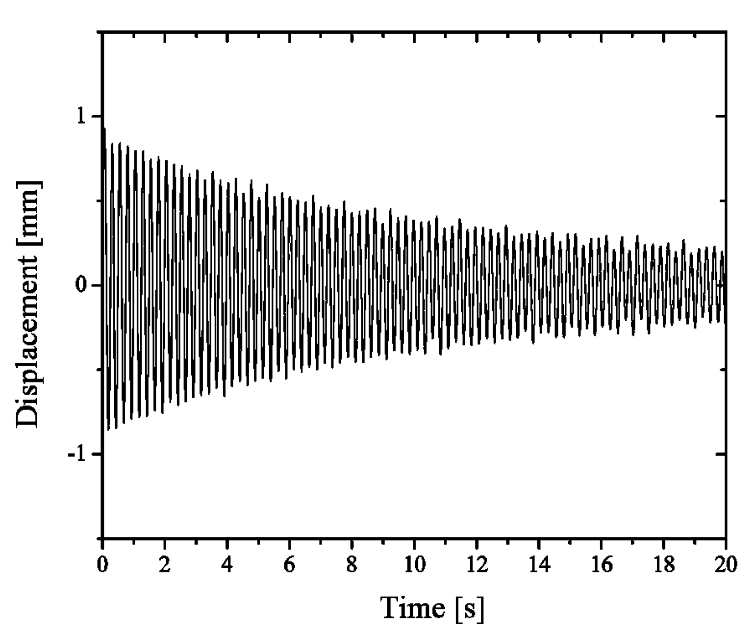
Figure 9 shows the time history plot of the excitation force. Figure 10 shows the 20 s of displacement response curve at Point A after the excitation. As can be seen from Figure 10, attenuation vibration occurred around the equilibrium position of the system after the excitation force was applied; the vibration amplitude attenuated nearly in a geometrical manner, and the vibration period increased slightly with the decrease in amplitude. The amplitude attenuation can be attributed to the damping and friction in the joint structure as well as the material damping of the beam structure. The change in the vibration period can be attributed to the damping and nonlinear stiffness of the joint structure as well as the material damping of the beam structure.

5.2. Numerical Simulation and Analysis

The finite element model of the above experimental system was established by using ANSYS, and transient dynamic analysis was performed. In the model, BEAM4 is used as the beam element; MASS21 is used as the lumped mass; COMBIN7 nonlinear spring unit, which can be used to simulate the nonlinear elastic force and Coulomb friction force in the joint structure, is used as the inter-panel joint. The assignment of dynamic parameters for the COMBIN7 is based on the results of dynamic parameter identification for the inter-panel joint given in Section 3. In addition, the dimensions, material parameters, and constraints of each part of the finite element model are all consistent with the experimental conditions. According to the force applying method used in the experiment, the impulsive force, 65 N for 0.005 s, was applied to the finite element model. Transient dynamic analysis was performed to obtain the response of the model.

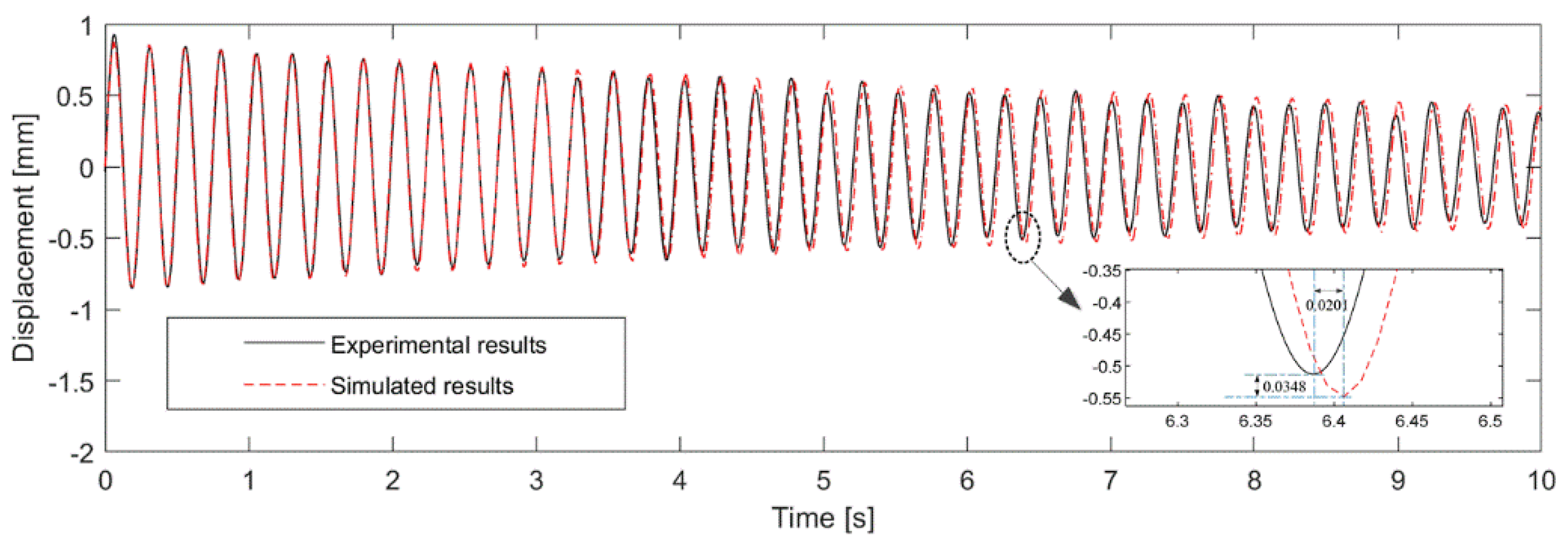
Simulated results of displacement response at Point A were compared with the experimental results. Figure 11 shows the comparison of displacement response results in the first 10 s. As shown in Figure 11, the vibration period and amplitude of the two displacement response curves are in good agreement, and attenuation of the amplitude with time is basically in the same manner. Furthermore, the RMS error of the displacement response amplitude between the two curves is 0.035 in the first 20 s, and the mean difference of the vibration period is 0.018 s. The above comparison and analysis show that the simulated results of vibration response are basically consistent with the experimental results, indicating that the finite element model established on the basis of the dynamic equation of the inter-panel joint given in Section 3 can accurately describe nonlinear dynamic behaviors of real inter-panel joints. The vibration response results obtained by the model are close to experimental results. So, the validity of the established dynamic equation of the joints and the feasibility of the joint modeling method are proved.

6. Conclusions

With a view to the nonlinear dynamic properties of the joints in deployable mechanisms of spacecraft, multiple linear and nonlinear dynamic parameters of the joints at the root of solar panels and between solar panels were identified by using the force state mapping method and dynamic experiment data of real joints. Based on that, the nonlinear dynamic model of the joints was established. The validity of the model has been verified by vibration tests under pulsed excitation. Because real complex nonlinear joints on spacecraft were used in the dynamic experiment and a nonlinear system identification method was employed to identify a variety of dynamic parameters from the experimental data, the model can reflect the nonlinear stiffness, friction, and damping characteristics of the real joints. The method of establishing the dynamic model of the nonlinear joints on solar panels is applicable for other connecting structures in spacecraft. The established model can serve as a theoretical reference for further analysis of the dynamic characteristics of deployable mechanisms on spacecraft.

References

- Crawley, E.F. Nonlinear characteristics of joints as elements of multi-body dynamic systems. In Proceedings of the Workshop on Computational Methods for Structural Mechanics and Dynamics, NASA Langley Research Center, Hampton, VA, USA, 19–21 June 1985. [Google Scholar]
- Ren, Y.; Beards, C.F. Identification of effective linear joints using coupling and joint identification techniques. J. Vib. Acoust. 1998, 120, 331–338. [Google Scholar]
- Wang, M.; Wang, D.; Zheng, G.T. Joint dynamic properties identification with partially measured frequency response function. Mech. Syst. Signal Process. 2012, 27, 499–512. [Google Scholar]
- Boswald, M.; Link, M. Identification of non-linear joint parameters by using frequency response residuals. In Proceedings of the International Conference on Noise Vibration Engineering, Leuven, Belgium, 20–22 September 2004; pp. 3121–3140. [Google Scholar]
- Subudhi, B.; Jena, D. A differential evolution based neural network approach to nonlinear system identification. Appl. Soft Comput. 2011, 11, 861–871. [Google Scholar]
- Lee, Y.S.; Tsakirtzis, S.; Vakakis, A.F.; Bergman, L.A.; McFarland, D.M. A time-domain nonlinear system identification method based on multiscale dynamic partitions. Meccanica 2011, 46, 625–649. [Google Scholar]
- Grauer, J.A.; Boucher, M.J. Identification of aeroelastic models for the X-56a longitudinal dynamics using multisine inputs and output error in the frequency domain. Aerospace 2019, 6, 24. [Google Scholar]
- Crawley, E.F.; Aubert, A.C. Identification of nonlinear structural elements by force-state mapping. AIAA J. 1986, 24, 155–162. [Google Scholar]
- Crawley, E.F.; O’Donnell, K.J. Force-state mapping identification of nonlinear joints. AIAA J. 1987, 25, 740–749. [Google Scholar]
- Kim, W.J.; Park, Y.S. Non-linear joint parameter identification by applying the force-state mapping technique in the frequency domain. Mech. Syst. Signal Process. 1994, 8, 519–529. [Google Scholar]
- Masters, B.P.; Crawley, E.F. Multiple degree-of-freedom force-state component identification. AIAA J. 1994, 32, 2276–2285. [Google Scholar]
- Meskell, C.; Fitzpatrick, J.A.; Rice, H.J. Application of force-state mapping to a non-linear fluid-elastic system. Mech. Syst. Signal Process. 2001, 15, 75–85. [Google Scholar]
- Namdeo, V.; Manohar, C.S. Force state maps using reproducing kernel particle method and kriging based functional representations. Comput. Model. Eng. Sci. 2008, 32, 123–159. [Google Scholar]
- Mehrpouya, M.; Graham, E.; Park, S.S. FRF based joint dynamics modeling and identification. Mech. Syst. Signal Process. 2013, 39, 265–279. [Google Scholar]
- Li, H.Q.; Yu, Z.W.; Guo, S.J.; Cai, G.P. Investigation of joint clearances in a large-scale flexible solar array system. Multibody Syst. Dyn. 2018, 3, 227–292. [Google Scholar]
- Bai, Z.; Zhao, J. A study on dynamic characteristics of satellite antenna system considering 3D revolute clearance joint. Int. J. Aerosp. Eng. 2020, 2020, 8846177. [Google Scholar]
- Li, Y.; Yang, Y.; Li, M.; Liu, Y.; Huang, Y. Dynamics analysis and wear prediction of rigid-flexible coupling deployable solar array system with clearance joints considering solid lubrication. Mech. Syst. Signal Process. 2022, 162, 108059. [Google Scholar]
- Ma, X.; Li, T.; Ma, J.; Wang, Z.; Shi, C.; Zheng, S.; Cui, Q.; Li, X.; Liu, F.; Guo, H.; et al. Recent advances in space-deployable structures in China. Engineering 2022, 4, 13. [Google Scholar]
- Jorgensen, C.A. International Space Station Evolution Data Book; NASA/SP-2000-6109/VOL2/REV1; FDC/NYMA: Hampton, Virgini, 2000; Volume 2. [Google Scholar]