Article

A Strong Form Meshless Method for the Solution of FGM Plates

Institute of Construction and Architecture, Slovak Academy of Sciences, Dubravska cesta 9, 845 03 Bratislava, Slovakia
*
Author to whom correspondence should be addressed.
Aerospace 2022, 9(8), 425; https://doi.org/10.3390/aerospace9080425
Submission received: 27 May 2022 / Revised: 29 July 2022 / Accepted: 1 August 2022 / Published: 4 August 2022
(This article belongs to the Special Issue Recent Advances in Computational Mechanics)

Abstract

:
Laminated composite structures suffer from failure because of concentrations of gradient fields on interfaces due to discontinuity of material properties. The rapid development of material science enables designers to replace classical laminated plate elements in aerospace structures with more advanced ones made of functionally graded materials (FGM), which are microscopic composite materials with continuous variation of material coefficients according to the contents of their micro-constituents. Utilization of FGM eliminates the inconvenience of laminated structures but gives rise to substantial changes in structural design This paper deals with the presentation of a strong formulation meshless method for the solution of FGM composite plates. Recall that the fourth-order derivatives of deflections are involved in the governing equations for plate structures. However, the high-order derivatives of field variables in partial differential equations (PDE) lead to increasing inaccuracy of approximations. For that reason, the decomposition of the high-order governing equations into the second-order PDE is proposed. For the spatial approximation of field variables, the meshless moving least square (MLS) approximation technique is employed. The reliability (numerical stability, convergence, and accuracy) as well as computational efficiency of the developed method is illustrated by several numerical investigations of the response of FGM plates with the transversal gradation of material coefficients under stationary and/or transient mechanical and thermal loadings.

1. Introduction

With the development of advanced composite materials, their application within aerospace engineering has become more widespread, and laminated composite plates are used as fundamental structural elements [1,2,3,4,5,6,7,8]. However, the discontinuities of material coefficients on the interfaces between two or more layers with different material properties can lead to concentrations of gradient fields and also to catastrophic failure of aerospace structures [9,10,11]. To overcome the problem of the delamination of laminated composite plates the functionally graded materials (FGM) are looking like promising alternatives of laminated structures. Due to the great potential in several branches of engineering applications, the FGMs are in the focus of researchers, which can be confirmed by a huge number of papers devoted to analyses with using various plate bending theories for FGM plates under static and/or dynamic loadings [12,13,14,15,16,17,18,19,20,21,22,23,24,25,26,27]. FGM structure can be characterized as a composite fabricated by mixing two or more different material micro-constituents [28,29]. In continuum models, the effective material properties, such as elastic modulus, Poisson’s ratio, mass density, etc., of the functionally graded composites are determined by the volume fraction distribution of the dispersed phases. In the literature several approaches are available for FGM modeling, such as the Mori–Tanaka scheme [30,31], composite cylindrical assemblage model [32,33], the simplified strength of materials method [34,35], and one of the most frequently used approach the rule of mixture where the material coefficients of multiphase materials are related directly to the volume fractions and individual coefficients of the constituents [36,37].
Despite FGMs being microscopically highly non-homogeneous structures, they exhibit continuous properties changing smoothly with respect to the spatial coordinates in macro-structural elements. The continuum models of FGM have been widely used in many engineering applications, for instance, the static behavior of FG rectangular plates was studied by Reddy [16], and also an axisymmetric formulation for circular and annular FG plate bending was observed [38] within the third-order shear deformation plate theory. Xu and Zhou [39] studied rectangular FG plates with variable plate thickness and exponential gradation of elastic modulus in the lateral direction as a 3D problem.
In the last three decades, the meshless formulations have become an attractive alternative to classical mesh-based discretization methods (such as FEM, BEM, etc.), because of various advantages [40] resulting from the fact that only nodes are used for approximation instead of elements and no elements are needed for background integration like in the element-free Galerkin (EFG) method [41,42]. Additional advantages of the meshless formulations arise in numerical solutions of boundary value problems for partial differential equations (PDE) with variable coefficients like in the case of functionally graded materials (FGM), since the complexity is not increased as compared with the case of homogeneous media. The maximum order of spatial derivatives in weak formulations is lower by one than the order of governing PDE.
The main drawback of meshless methods is the worse computational efficiency than that in mesh-based methods because the shape functions are not expressed as elementary function. This handicap is solved in the present paper by decreasing the number of evaluations of shape functions by using the strong formulation, which can be shown to be a limit case of local weak formulations with approaching the size of the local subdomain to zero. The decrease in the accuracy of approximation of high-order derivatives in plate bending problems is overcome by decomposition of governing equations into governing equations with lower-order derivatives. This is performed at the price of an increase in nodal unknowns. The moving least square (MLS) approximation scheme [43] with using the so-called central approximation node (CAN) concept [44,45] is employed for approximation of field variables. In regards to the numerical evaluation of the derivatives of field variables, we shall use the standard as well as the modified differentiation [46,47] with using not higher than first-order derivatives of shape functions even for higher-order derivatives of field variables. Numerical tests for accuracy and computational efficiency of these approaches are presented in this paper. Moreover, the modified evaluation of the shape functions and their derivatives will be employed [46,47] in order to obey correctly the requirement of completeness of the used set of shape functions. The accuracy and convergence study is accomplished on boundary value problems for bending of thin rectangular FGM plate, where the exact solutions are available and can be used as the benchmark solutions. The attention is paid also to numerical parametric study with respect to various parameters of gradations of the material coefficients of the FGM plates. Several numerical examples are presented to investigate the static and transient response of elastic FGM plates, and thermomechanical response of the FGM plates with transversal and/or in-plane gradation of material properties under stationary and/or transient mechanical and thermal loadings. The main goal of this paper is to present a well-developed computational method (with attributes mentioned in the previous paragraph) for a broad class of plate bending problems. The functional dependence of material coefficients (such as Young modulus, mass density, specific heat capacity, thermal expansion, heat conduction coefficient) gives rise to coupling effects among the field variables including the interaction between the in-plane deformation and bending modes. The unified formulation covers three different kinds of deformation assumptions known as the classical Kirchhoff–Love theory for thin plate bending, the first-order shear deformation theory and the third-order shear deformation theory. The governing equations and possible boundary conditions are developed from the variation principles. In Section 2.1, the formulation is derived for FGM elastic plates under static and/or dynamic loadings. The coupled thermoelastic problems are considered in Section 2.2. Section 3 is devoted to numerical implementation of meshless discretization with using strong formulation and the MLS approximation for spatial dependence of field variables. Finally, in Section 4, we present illustrative examples in order to demonstrate the reliability of the computational method, its universality and discuss the coupling phenomena within three various plate bending theories.

2. Governing Equations

2.1. Governing Equation for Elastic FGM Plates

In this chapter, we shall derive the unified formulation for all three plate bending theories, such as the Kirchhoff–Love theory (KLT), the first-order shear deformation plate theory (FSDPT), and the third-order shear deformation plate theory (TSDPT), in which the displacement field v i ( x , x 3 , t ) can be expressed in terms of the in-plane displacements u α ( x , t ) , transversal deflections w ( x , t ) and rotations of the normal to the mid-surface φ α ( x , t ) by
v i ( x , x 3 , t ) = δ i α u α ( x , t ) + c 1 ϕ ( x 3 ) x 3 w , α ( x , t ) + c 1 ϕ ( x 3 ) φ α ( x , t ) + δ i 3 w ( x , t )
where i = 1 , 2 , 3 , α = 1 , 2 , ϕ ( x 3 ) : = x 3 c 2 ψ ( x 3 ) , ψ ( x 3 ) : = 4 3 x 3 h 2 x 3 , x 3 h / 2 , h / 2 , x Ω , with Ω being the plate area in the mid-surface (Figure 1).
The key factors c 1 and c 2 in Equation (1) were introduced for the proper selection among various plate bending theories within the unified formulation, and are specified as:
(i)
for KLT: c 1 = 0 , c 2 = 0 ,
(ii)
for FSDPT: c 1 = 1 , c 2 = 0 ,
(iii)
for TSDPT: c 1 = 1 , c 2 = 1 .
According to the Hooke law, the 3D stresses in the linear elastic and isotropic continuum are given as
σ i j ( x , x 3 , t ) = E 1 ν 2 1 ν H H e i j ( x , x 3 , t ) + ν δ i j e k k ( x , x 3 , t )
where E , ν stand for the elastic modulus and Poisson’s ratio, respectively. The total strains are expressed as e i j = v i , j + v j , i / 2 , while
H = 1 χ ν ,   χ = 1 , for       p l a n e s t r e s s p r o b l e m s 2 , for       3 D p r o b l e m s   o r p l a n e s t r a i n
By substitution of Equation (1) into Equation (2), the stresses inside an elastic plate considered within three plate bending theories are obtained
σ α β ( x , x 3 , t ) = E 1 ν 2 1 ν H τ α β ( u ) ( x , t ) + c 1 ϕ ( x 3 ) τ α β ( φ ) ( x , t ) + c 1 ϕ ( x 3 ) x 3 τ α β ( w ) ( x , t )
σ α 3 ( x , x 3 , t ) = E 1 + ν c 1 2 ϕ ( x 3 ) w , α ( x , t ) + φ α ( x , t ) ,   ϕ ( x 3 ) = 3 ϕ ( x 3 )
σ 33 ( x , x 3 , t ) = E ν 1 ν 2 1 ν H u γ , γ ( x , t ) + c 1 ϕ ( x 3 ) φ γ , γ ( x , t ) + c 1 ϕ ( x 3 ) x 3 w , γ γ ( x , t )
in which the strain contributions associated with in-plane displacements, rotations, and transversal displacements (deflections) are
τ α β ( u ) ( x , t ) : = H ε α β ( x , t ) + ν δ α β ε γ γ ( x , t ) , τ α β ( φ ) ( x , t ) : = H η α β ( x , t ) + ν δ α β η γ γ ( x , t )
τ α β ( w ) ( x , t ) : = H w , α β ( x , t ) + ν δ α β w , γ γ ( x , t )
with ε α β = u α , β + u β , α / 2 , η α β = φ α , β + φ β , α / 2 .
Within this paper, we utilize the Einstein summation rule with respect to repeated subscripts, and the comma preceding a subscript denotes the derivative with respect to the corresponding coordinate. Thus,
w ( x ) , γ γ = w , 11 ( x ) + w , 22 ( x ) = 2 w ( x ) x 1 x 1 + 2 w ( x ) x 2 x 2
Making use of the rule of mixture for micro-composites with two constituents, one can obtain material properties for FGM plates with power law gradation in the transversal direction as
E ( x , x 3 ) = E 0 E H ( x ) E V ( x 3 ) ,   E V ( x 3 ) = 1 + ζ 1 2 ± x 3 h p
ρ ( x , x 3 ) = ρ 0 ρ H ( x ) ρ V ( x 3 ) ,   ρ V ( x 3 ) = 1 + ε 1 2 ± x 3 h g
where the Young modulus E , and mass density ρ are factorized using the subscript 0, H, V for the reference values, factors responsible for in-plane (horizontal) gradation and transversal gradation, respectively. The levels of gradation are determined by ζ and ε , while p and g are exponents of the power law gradations. In addition, the thickness of the FGM plate is allowed to be variable, h ( x ) .
For the derivation of the equations of motion together with the boundary and initial conditions for mechanical fields, Hamilton’s principle is utilized
δ U δ W e δ K = 0
where the variations of the elastic deformation energy, the kinetic energy, and the energy of external transversal forces are expressed as
δ U = 0 T Ω h / 2 h / 2 σ i j ( x , x 3 , t ) δ e i j ( x , x 3 , t ) d x 3 d Ω d t
δ K = 0 T Ω h / 2 h / 2 ρ v ˙ i δ v ˙ i d x 3 d Ω d t
δ W e = 0 T Ω t 3 ( x , t ) δ w ( x , t ) d Ω d t
in which T is the considered time period.
The time derivative of field variables is marked by a dot over the variable. Performing the integrations in a transversal direction, we obtain
δ U = 0 T Ω T α β ( x , t ) δ u α , β ( x , t ) M α β ( w ) ( x , t ) δ w , α β ( x , t ) + M α β ( φ ) ( x , t ) δ φ α , β ( x , t ) + + T 3 β ( w φ ) ( x , t ) δ w , β ( x , t ) + δ φ β ( x , t ) d Ω d t
δ K = 0 T Ω I ˜ ( u u ) ( x ) u ¨ β ( x , t ) + I ˜ ( u φ ) ( x ) φ ¨ β ( x , t ) + I ˜ ( u w ) ( x ) w ¨ , β ( x , t ) δ u β ( x , t ) + + I ˜ ( φ u ) ( x ) u ¨ β ( x , t ) + I ˜ ( φ φ ) ( x ) φ ¨ β ( x , t ) + I ˜ ( φ w ) ( x ) w ¨ , β ( x , t ) δ φ β ( x , t ) + + I ˜ ( w u ) ( x ) u ¨ β ( x , t ) + I ˜ ( w φ ) ( x ) φ ¨ β ( x , t ) + I ˜ 2 ( w w ) ( x ) w ¨ , β ( x , t ) δ w , β ( x , t ) + + I ˜ 1 ( w w ) ( x ) w ¨ ( x , t ) δ w ( x , t ) d Ω d t
where the following integral quantities for in-plane stresses
T α β ( x , t ) : = h / 2 h / 2 σ α β ( x , x 3 , t ) d x 3
stress couples
M α β ( φ ) ( x , t ) : = c 1 h / 2 h / 2 ϕ ( x 3 ) σ α β ( x , x 3 , t ) d x 3 ,   M α β ( w ) ( x , t ) : = h / 2 h / 2 x 3 σ α β ( x , x 3 , t ) d x 3 M α β ( φ ) ( x , t )
and shear stresses
T 3 β ( w φ ) ( x , t ) : = c 1 h / 2 h / 2 1 c 2 κ + c 2 c 2 ψ ( x 3 ) σ 3 β ( x , x 3 , t ) d x 3
represent the considered fields averaged through the plate thickness.
The mass inertia terms are defined as
I ˜ u u , I ˜ u φ , I ˜ u w = h / 2 h / 2 1 , c 1 ϕ ( x 3 ) , c 1 ϕ ( x 3 ) x 3 ρ ( x 3 ) d x 3
I ˜ φ u , I ˜ φ φ , I ˜ φ w = h / 2 h / 2 c 1 ϕ ( x 3 ) , c 1 ϕ 2 ( x 3 ) , c 1 ϕ 2 ( x 3 ) x 3 ϕ ( x 3 ) ρ ( x 3 ) d x 3
I ˜ w u , I ˜ w φ , I ˜ 1 w w , I ˜ 2 w w = = h / 2 h / 2 c 1 ϕ ( x 3 ) x 3 , c 1 ϕ 2 ( x 3 ) x 3 ϕ ( x 3 ) , 1 , c 1 ϕ ( x 3 ) x 3 2 ρ ( x 3 ) d x 3
The shear correction factor, κ , represents the Reissner modification of the shear stresses in the case of the FSDPT. During the derivation of Equation (11), we were keeping in mind that the variations δ u β , δ φ β , δ w are vanishing at t = 0 and t = T , hence δ w , β ( x , t = 0 ) = 0 and δ w , β ( x , t = T ) = 0 as well. The explicit expressions for the averaged fields defined by Equations (12)–(14) and mass inertia terms defined by Equation (15) can be found in [48].
Certain rearrangements [48,49] in δ U δ W can lead to expression without derivatives of variations of field variables. Then, the set of governing equations at x Ω , t [ 0 , T ] and restrictions on the boundary edge Ω at t [ 0 , T ] are obtained:
governing equations
T α β , β ( x , t ) + I ˜ ( u u ) ( x ) u ¨ α ( x , t ) + I ˜ ( u φ ) ( x ) φ ¨ α ( x , t ) + I ˜ ( u w ) ( x ) w ¨ , α ( x , t ) = 0
M α β , α β ( w ) ( x , t ) + T 3 β , β ( w φ ) ( x , t ) + + I ˜ 1 ( w w ) ( x ) w ¨ ( x , t ) I ˜ ( w u ) ( x ) u ¨ β ( x , t ) + I ˜ ( w φ ) ( x ) φ ¨ β ( x , t ) + I ˜ 2 ( w w ) ( x ) w ¨ , β ( x , t ) , β = t 3 ( x , t )
M α β , β ( φ ) ( x , t ) T 3 α ( w φ ) ( x , t ) + I ˜ ( φ u ) ( x ) u ¨ α ( x , t ) + I ˜ ( φ φ ) ( x ) φ ¨ α ( x , t ) + I ˜ ( φ w ) ( x ) w ¨ , α ( x , t ) = 0
boundary restrictions
n β ( x ) T α β ( x , t ) δ u α ( x , t ) = 0
n α ( x ) n β ( x ) M α β ( w ) ( x , t ) δ w n ( x , t ) = 0
n β ( x ) M α β ( φ ) ( x , t ) δ φ α ( x , t ) = 0
V ( x , t ) n β ( x ) I ˜ ( w u ) ( x ) u ¨ β ( x , t ) + I ˜ ( w φ ) ( x ) φ ¨ β ( x , t ) + I ˜ 2 ( w w ) ( x ) w ¨ , β ( x , t ) δ w ( x , t ) = 0
where
V ( x , t ) : = n α ( x ) M α β , β ( w ) ( x , t ) + T 3 α ( w φ ) ( x , t ) + t T ( w ) ( x , t ) c δ ( x x c ) T ( w ) ( x c , t )
is the generalized shear force, T ( w ) ( x , t ) : = t α ( x ) n β ( x ) M α β ( w ) ( x , t ) is the twisting moment defined on the plate edge Ω . Furthermore, the jump at a corner on the oriented boundary edge Ω is defined as
A ( x c ) : = A ( x c 0 ) A ( x c + 0 )
It is appropriate to introduce the dimensionless fields
u β ( x , t ) : = u β ( x , t ) h 0 ,   φ β ( x , t ) : = φ β ( x , t ) ,   w ( x , t ) : = w ( x , t ) h 0
in which the dimensionless variables are defined as
x β : = x β L ,   x 3 : = x 3 h 0 = h ( x ) z ,   h ( x ) = h 0 h ( x ) ,   t : = t T
where L is the characteristic length for the in-plane dimensions and h 0 is the thickness of the plate.
In what follows, for simplicity, we shall write g ( x , t ) instead of g ( x , t ) .
Substituting Equations (18) and (19) into Equation (16), one can obtain the governing equation in sense of dimensionless formulation
T α β , β ( x , t ) + I ( u u ) ( x ) u ¨ α ( x , t ) + I ( u φ ) ( x ) φ ¨ α ( x , t ) + I ( u w ) ( x ) w ¨ , α ( x , t ) = 0
M α β , α β ( w ) ( x , t ) + L h 0 2 T 3 β , β ( w φ ) ( x , t ) + I 1 ( w w ) ( x ) w ¨ ( x , t ) I ( w u ) ( x ) u ¨ β ( x , t ) + I ( w φ ) ( x ) φ ¨ β ( x , t ) + I 2 ( w w ) ( x ) w ¨ , β ( x , t ) , β = t 3 ( x , t )
M α β , β ( φ ) ( x , t ) L h 0 2 T 3 α ( w φ ) ( x , t ) + I ( φ u ) ( x ) u ¨ α ( x , t ) + I ( φ φ ) ( x ) φ ¨ α ( x , t ) + I ( φ w ) ( x ) w ¨ , α ( x , t ) = 0
The dimensionless transversal mechanical loading is defined as t 3 ( x , t ) : = L 4 / D 0 h 0 t 3 ( x , t ) , where D 0 = E 0 ( h 0 ) 3 12 ( 1 ν 2 ) is the bending stiffness. For elastodynamic plate bending problems, the explicit expressions for the semi-integral fields (12)–(14) and the mass inertia coefficients (15) are given in [48]. The boundary restrictions are obtained from (17) by replacing all fields and mass inertia coefficients by their dimensionless counterparts.
In Equation (20) the fourth-order derivatives of transversal deflections and third-order derivatives of in-plane displacements and rotations are included, which can lead to a reduction in the accuracy of approximations of high-order derivatives of field variables. To overcome this shortcoming, we employ the decomposition technique on the derived set of the partial differential equations (PDE) by introducing additional field variables
m ( x , t ) : = 2 w ( x , t ) ,   s α ( x , t ) : = 2 u α ( x , t ) ,   f α ( x , t ) : = 2 φ α ( x , t )
Then, the final set of governing equations for primary field variables w ( x , t ) , m ( x , t ) , u β ( x , t ) , s β ( x , t ) , φ β ( x , t ) , f β ( x , t ) is given by Equations (20) and (21), which include derivatives not higher than second-order [47].

2.2. Governing Equation for Thermoelastic FGM Plates

Similarly, like in the previous chapter, we shall derive the governing equation for the FGM plates under thermal loadings. Within the linear thermoelastic and isotropic media, the 3D stresses are given as
σ i j ( x , x 3 , t ) = E 1 ν 2 1 ν H H e i j ( x , x 3 , t ) + ν δ i j e k k ( x , x 3 , t ) α ( 1 + ν ) θ ( x , x 3 , t ) θ 0 δ i j
where E , ν , α denote the elastic modulus, Poisson’s ratio, and the linear thermal expansion coefficient, respectively.
Furthermore, θ , θ 0 and e i j stand for the temperature, reference temperature, and total strains, respectively.
By substitution of Equation (1) into Equation (22), the stresses inside an elastic plate considered within three plate bending theories are obtained as
σ α β ( x , x 3 , t ) = E 1 ν 2 1 ν H τ α β ( u ) ( x , t ) + c 1 ϕ ( x 3 ) τ α β ( φ ) ( x , t ) + c 1 ϕ ( x 3 ) x 3 τ α β ( w ) ( x , t ) α δ α β τ ( θ ) ( x , x 3 , t )
σ α 3 ( x , x 3 , t ) = E 1 + ν c 1 2 ϕ ( x 3 ) w , α ( x , t ) + φ α ( x , t )
σ 33 ( x , x 3 , t ) = E ν 1 ν 2 1 ν H u γ , γ ( x , t ) + c 1 ϕ ( x 3 ) φ γ , γ ( x , t ) + c 1 ϕ ( x 3 ) x 3 w , γ γ ( x , t ) α ν τ ( θ ) ( x , x 3 , t )
in which the strain contributions associated with in-plane displacements, rotations, and transversal deflections τ α β ( u ) ( x , t ) , τ α β ( φ ) ( x , t ) , τ α β ( w ) ( x , t ) are defined by Equation (5) and the temperature contribution is
τ ( θ ) ( x , x 3 , t ) : = ( 1 + ν ) θ ( x , x 3 , t ) θ 0
The power law gradation in the transversal direction for material coefficients such as elastic modulus, thermal expansion coefficient, heat conduction coefficients, specific heat capacity, and mass density is defined by the following relations:
E ( x , x 3 ) = E 0 E H ( x ) E V ( x 3 ) ,   E V ( x 3 ) = 1 + ζ 1 2 ± x 3 h p
α ( x , x 3 ) = α 0 α H ( x ) α V ( x 3 ) ,   α V ( x 3 ) = 1 + ξ 1 2 ± x 3 h r
k ( x , x 3 ) = k 0 k H ( x ) k V ( x 3 ) ,   k V ( x 3 ) = 1 + ω 1 2 ± x 3 h s ,
c ( x , x 3 ) = c 0 c H ( x ) c V ( x 3 ) ,   c V ( x 3 ) = 1 + χ 1 2 ± x 3 h q ,
ρ ( x , x 3 ) = ρ 0 ρ H ( x ) ρ V ( x 3 ) ,   ρ V ( x 3 ) = 1 + ε 1 2 ± x 3 h g
The parameters ζ , ξ , ω , χ ε stand for the levels of power law gradations in transversal direction, while p , r , s , q , g are exponents of these gradations.
In order to develop the formulation consistent with elastic deformation assumptions (with the known x 3 -dependence), we approximate the temperature field by the second-order power series expansion with respect to the x 3 -coordinate as
θ ( x , x 3 , t ) θ 0 + ϑ 0 ( x , t ) + z ϑ 1 ( x , t ) + z 2 ϑ 2 ( x , t ) ,   z = x 3 h [ 0.5 , 0.5 ]
where ϑ s ( x , t ) are a new field variables with s = 0 , 1 , 2 . Then, one can write
τ ( θ ) ( x , x 3 , t ) = s = 0 2 z s τ ( ϑ s ) ( x , t ) ,   τ ( ϑ s ) ( x , t ) : = ( 1 + ν ) ϑ s ( x , t )
The governing equations and the boundary restrictions for mechanical fields are formally given by Equations (16) and (17), respectively. Recall that in case of thermoelasticity, the semi-integral fields (12)–(14) include also thermal contributions [49] in contrast to case of elastodynamics. In the governing Equation (16), we have only five PDEs for eight independent field variables, which means we need three more equations to complete the set of governing equations for FGM plate bending problems in classical thermoelasticity.
The heat conduction equation within coupled classical thermoelasticity is given by
k θ , j , j ρ c θ ˙ E α H θ 0 v ˙ j , j = 0
in which k , ρ , and c is the heat conduction coefficient, mass density, and the specific heat capacity, respectively.
In view of the previously introduced three field variables ϑ s ( x , t ) , the heat conduction equation is still dependent on x 3 as
k H ( x ) k V ( x 3 ) s = 0 2 z s ϑ s ( x , t ) , j , j ρ 0 c 0 k 0 ρ H ( x ) ρ V ( x 3 ) c H ( x ) c V ( x 3 ) s = 0 2 z s ϑ ˙ s ( x , t ) E 0 α 0 k 0 H E H ( x ) E V ( x 3 ) α H ( x ) α V ( x 3 ) θ 0 v ˙ β , β ( x , x 3 , t ) = 0
In order to accomplish the 2D formulation, we propose to integrate Equation (29) through the thickness of the plate with getting the heat conduction equation in an averaged sense
s = 1 2 C ( θ ϑ s ) ( x ) ϑ s ( x , t ) + s = 0 2 G β ( θ ϑ s ) ( x ) ϑ s , β ( x , t ) + s = 0 2 G ( θ ϑ s ) ( x ) ϑ s , β β ( x , t ) + + s = 0 2 I ( θ ϑ s ) ( x ) ϑ ˙ s ( x , t ) + C ( θ u ) ( x ) u ˙ β , β ( x , t ) + C ( θ w ) ( x ) w ˙ , β β ( x , t ) + C ( θ φ ) ( x ) φ ˙ β , β ( x , t ) = 0
For the details on coefficients C ( ) , G ( ) , and I ( ) see [50].
The dimensionless fields
u β ( x , t ) : = u β ( x , t ) h 0 ,   φ β ( x , t ) : = φ β ( x , t ) ,   w ( x , t ) : = w ( x , t ) h 0 ,   ϑ s ( x , t ) : = ϑ s ( x , t ) θ 0
are introduced by using the dimensionless variables as
x β : = x β L ,   x 3 : = x 3 h 0 = h ( x ) z ,   h ( x ) = h 0 h ( x ) ,   t : = t T
Furthermore, it is written g ( x , t ) instead of g ( x , t ) for the reason of simplicity.
The other two equations result from the 3D boundary conditions considered on the top and bottom surfaces of the plate. These BCs can be given by an arbitrary combination of the following boundary conditions
(i)
Dirichlet type:
ϑ 0 ( x , t ) ± 1 2 ϑ 1 ( x , t ) + 1 4 ϑ 2 ( x , t ) = θ ¯ ( x , ± h / 2 , t ) θ 0 1
(ii)
Neumann type:
± k 0 k H ( x ) k V ( ± 1 / 2 ) ϑ 1 ( x , t ) ± ϑ 2 ( x , t ) = q ¯ ( x , ± h / 2 , t ) / θ 0
(iii)
Robin type:
A 1 + ϑ 0 ( x , t ) ± 1 2 ϑ 1 ( x , t ) + 1 4 ϑ 2 ( x , t ) ± B k 0 k H ( x ) k V ( ± h / 2 ) ϑ 1 ( x , t ) ± ϑ 2 ( x , t ) = 0
The q ¯ ( x , ± h / 2 , t ) and θ ¯ ( x , ± h / 2 , t ) are the prescribed values of the heat flux and temperature on the top and bottom surfaces of the plate, respectively. Taking into account that, θ ( x , x 3 = 0 , t ) = θ 0 + ϑ 0 ( x , t ) , the boundary conditions on Ω can be given as
(i)
Dirichlet type:
ϑ 0 ( x , t ) Ω = θ ¯ ( x , x 3 = 0 , t ) / θ 0 1
(ii)
Neumann type:
k 0 k H ( x ) k V ( 0 ) n β ( x ) ϑ 0 , β ( x , t ) Ω = L / θ 0 q ¯ ( x , 0 , t )
(iii)
Robin type:
A ϑ 0 ( x , t ) Ω + B k 0 k H ( x ) k V ( 0 ) n β ( x ) ϑ 0 , β ( x , t ) Ω = 0
with θ ¯ ( x , x 3 = 0 , t ) and q ¯ ( x , 0 , t ) being the prescribed values of the temperature and heat flux on the boundary edge of the plate.
Substituting Equations (31) and (32) into Equation (16), one can obtain the dimensionless form of the governing equations which are formally the same as (20), but the semi-integral fields include also the thermal contributions [49].
Thus, the complete set of governing equations for field variables describing the process of plate bending in classical thermoelasticity is given by Equations (20) and (30) plus two equations properly selected from (33)–(35) according to prescribed thermal boundary conditions on the top and bottom of the plate. The possible boundary conditions result form (17) and (36)–(38).
To overcome the shortcoming of decreasing the accuracy of approximation due to high-order derivatives in governing equations we utilize the decomposition formulation introduced in Section 2.1.
Then, the final set of governing equations for primary field variables w ( x , t ) , m ( x , t ) , u β ( x , t ) , s β ( x , t ) , φ β ( x , t ) , f β ( x , t ) , ϑ 0 ( x , t ) , ϑ 1 ( x , t ) , ϑ 2 ( x , t ) is given by Equations (21), (30) and (35), which include derivatives not higher than the second-order [47].

3. Meshless Approximations of Field Variables by Moving Least Square Approximation

In this paper, we shall employ the central approximation node (CAN) concept of the standard MLS approximation. By considering x q as the CAN for the approximation at a point x the number of nodes implied into the approximation at x is reduced a-priori from N to N q , where N is the number of all nodes and N q is the number of nodes supporting the approximation at x q , i.e., the number of nodes in the set q = { x a ; w a ( x q ) > 0 } a = 1 N , where w a ( x ) is the weight function associated with the node x a and taken at the field point x . In this paper, we employ the Gaussian weights. The MLS-CAN approximation is given as
u ( x ) a = 1 N q u ^ a ¯ ϕ ( q , a ) ( x ) ,   a ¯ = n ( q , a )
where a ¯ is the global number of the a -th node from the N q nodal points, u ^ a is a nodal unknown different from the nodal value u ( x a ) , and ϕ a ( x ) is the shape function associated with the nodal point x a . Generally, the nearest node to the field point x is selected as the CAN node.
In this paper, we shall utilize two types for differentiation: (a) the standard approach (D0), and (b) the modified approach ( D 1 ) for the evaluation of derivatives of field variables.
Within the standard approach, the derivative of u ( x ) can be approximated by differentiating Equation (39), i.e.,
u , i ( x ) a = 1 N q u ^ a ¯ ϕ , i ( q , a ) ( x ) ,   u , i j ( x ) a = 1 N q u ^ a ¯ ϕ , i j ( q , a ) ( x ) ,   u , i j k ( x ) a = 1 N q u ^ a ¯ ϕ , i j k ( q , a ) ( x )
For the details on the shape functions and their derivatives see [47].
In the modified approach, the derivatives are approximated by using the MLS shape functions ϕ a ¯ ( x ) and nodal values u ^ h ¯ and the first-order derivatives of the MLS shape functions. So,
u , i ( x ) a = 1 N q u ^ i a ¯ ϕ ( q , a ) ( x ) ,   u , i j ( x ) a = 1 N q u ^ i j a ¯ ϕ ( q , a ) ( x ) ,   u , i j k ( x ) a = 1 N q u ^ i j k a ¯ ϕ ( q , a ) ( x ) .  
From (401), we have
u , i ( x c ) h = 1 N c u ^ h ¯ ϕ , i ( c , h ) ( x c ) = h = 1 N c f i c h u ^ h ¯ ,   with   h ¯ = n ( c , h ) ,   f i c h = ϕ , i ( c , h ) ( x c )
while from (411), we have
u , i ( x c ) a = 1 N c u ^ i a ¯ ϕ ( c , a ) ( x c ) = h = 1 N c e c a u ^ i a ¯ ,   with   a ¯ = n ( c , a ) ,   e c a = ϕ ( c , a ) ( x c )
Extending the definitions of matrices f i c h and e c a to all nodes as
E c d : = e c a , d = a ¯ 0 ,   d a ¯ ,   F i c g : = f i c a , g = a ¯ 0 ,   g a ¯ ,   with   a ¯ = n ( c , a ) ,   a { 1 , 2 , , N c }
The Equations (42) and (43) are rewritten as
u , i ( x c ) = d = 1 N E c d u ^ i d = g = 1 N F i c g u ^ g
hence,
u ^ i d = g = 1 N c = 1 N ( E 1 ) d c F i c g u ^ g = g = 1 N G i d g u ^ g ,   G i d g : = c = 1 N ( E 1 ) d c F i c g
Differentiating (411), one can obtain
u , i j ( x ) a = 1 N q u ^ i a ¯ ϕ , j ( q , a ) ( x ) u , i j ( x c ) a = 1 N c u ^ i a ¯ ϕ , j ( c , a ) ( x c ) = g = 1 N F j c g u ^ i g
From (412), we have
u , i j ( x c ) a = 1 N c u ^ i j a ¯ ϕ ( c , a ) ( x c ) = d = 1 N E c d u ^ i j d
and by comparison to (46) and (47), one can receive
u ^ i j d = g = 1 N c = 1 N ( E 1 ) d c F j c g u ^ i g = g = 1 N G j d g u ^ i g = g , h = 1 N G j d g G i g h u ^ h
where we employed the expression for u ^ i g by Equation (45).
In a similar way,
u ^ i j k d = g , b , h = 1 N G k d g G j g b G i b h u ^ h
Substituting Equations (45), (48) and (49), into Equation (41), one can obtain the relationship for modified evaluation of derivatives of primary field variables. In this D1 approach, only the first-order derivatives of the MLS shape function ϕ a ¯ ( x ) and nodal values u ^ h are utilized for the evaluation of higher-order derivatives of the approximated function. The evaluation of G i d g , due to the necessity of inversion of E c d can lead to the lower computational efficiency of the modified differentiation approach as compared with the standard differentiation approach. This is the cost, what we have to pay for better accuracy given by the modified differentiation approach.

4. Numerical Examples

In this chapter, we shall present the results for FGM elastic and/or thermoelastic square plates with the power law gradation of material coefficients. The main geometrical parameter is the length of all sides of the plate L = 1 m. The length to thickness ratio is L / h 0 = 50 . The sides of the FG plates are considered to be clamped. The material coefficients are graded according to Equation (6) and/or Equation (25), while Poisson’s ratio is considered to be constant ν = 0.3 .
The nodes utilized for the discretization of the analyzed domain are distributed uniformly. The distance between neighbour nodes is marked by δ . The other parameters in the MLS-CAN approximation technique are the radius of the interpolation domain ρ a = 3.001 δ and shape function parameter c a = δ . In all numerical experiments the cubic polynomial basis m = 10 is used.

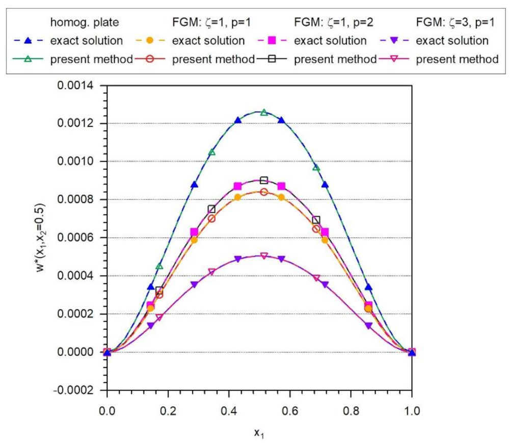
4.1. Verification of Presented Numerical Method
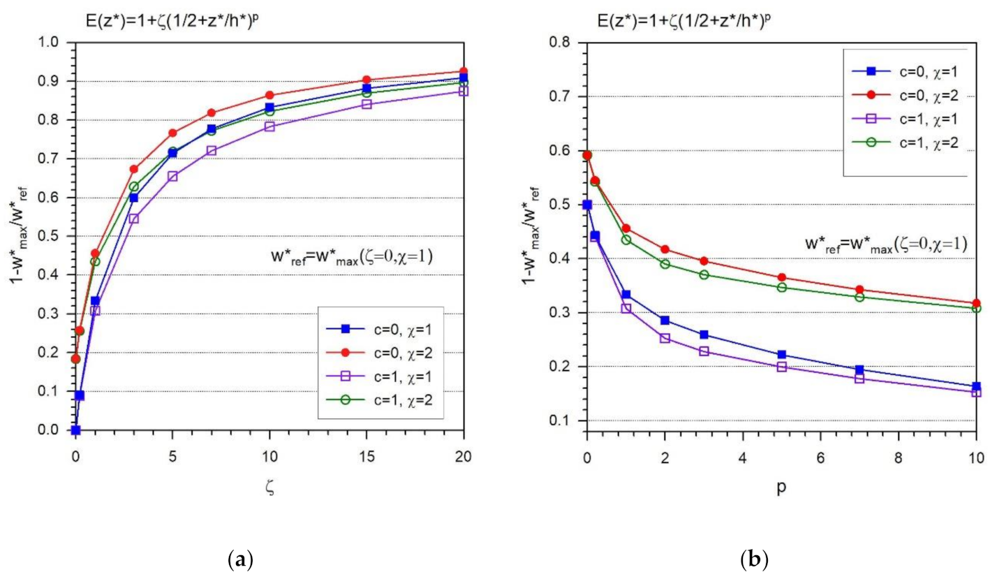
In the literature, we can easily find the analytical solution for clamped elastic square plates with constant bending stiffness [51]. For the study of the accuracy and convergence of the proposed computational method, the above-mentioned analytical solution will be utilized as benchmark solution. The error norm characterizing the accuracy of numerical solutions of BVP is given by
e r r o r = a = 1 N w ( x a ) w e x ( x a ) 2 1 / 2 a = 1 N w e x ( x a ) 2 1 / 2 100 ( % )
where N represents the number of all nodes within the discretized domain, w ( x a ) is the computed value of the field variable by the present method, while w e x ( x a ) is the exact value of the field variable at the nodal point x a .
First of all, to verify the proposed computational method, we shall present the comparison of results by the proposed method and the analytical solution by [51] for elastic plate bending problems. The homogeneous, as well as FGM square plates, are considered. The plates in all computations are subjected to uniform, stationary transversal loading q * = 1 . The power law transversal gradation of elastic modulus follows Equation (6), while elastic modulus at the bottom surface of the plate is E ( 0 ) = 120 × 10 9 Pa , the level of power law gradation ζ = 0 for the plate with constant bending stiffness, while ζ = 1 and ζ = 3 for the FGM plate with linear p = 1 and/or non-linear p = 2 transversal gradation, respectively. In Figure 2. it is seen that the results for the deflections by the present computational method are in excellent agreement with the analytical results [51].
A study on the accuracy, convergence, and computational efficiency of the present method was carried out too. The results of such investigation are shown in Figure 3. Good convergence rates are achieved by both employed differentiation techniques with increasing the number of nodes, i.e., with decreasing parameter δ. In regards to the computational efficiency, from Figure 3b it is clearly seen that in the case of the modified differentiation (D1) the computational time is not increased significantly, as compared to standard differentiation (D0).
As regards the comparison of the computational efficiency of the strong vs. weak formulations using the same number of nodes, it depends also on the amount of discretized equations [46,52]. The total computational time is composed of the time needed for creation of the system matrix ( t s m ) and the time needed for solution of the system of discretized equations ( t s o l ). Both the t s m and t s o l are increasing with increasing the amount of nodes, and t s m is approximately 10 times smaller in strong formulation than in case of weak formulation, while t s o l is independent on the kind of discretization. Thus, the computational efficiency of the strong formulation is ever better than that of the weak formulation, but the differences are diminishing with increasing the number of nodes when t s o l is becoming dominant.

4.2. Study of w u i Coupling in FGM Plates under Static Mechanical Loading

Now, we shall consider the FGM plate under static mechanical loading q * = 1 , t = 0 (the acceleration terms of Equation (20) are equal to zero).
First, we shall investigate the FGM plate with the transversal power law gradation of elastic modulus, focusing on the effect of w u i coupling. According to [49], it is evident that the coefficients C ( u w ) , C ( u φ ) , C ( w u ) , C ( w φ ) , responsible for coupling between in-plane displacements u α and bending measures (transversal deflections w and rotations φ α ), are proportional to the parameter ζ and vanish in homogeneous plates, where ζ = 0 . In order to assess the effect of material gradation on the w u i coupling, we introduce the multiplication factor c in the above coupling coefficients by replacing C ( · · ) with c C ( · · ) . Then, the value c = 1 corresponds to the real physical FGM plate, while c = 0 corresponds to the artificial situation when the w u i coupling in the FGM plate is switched off. Furthermore, the plane stress ( χ = 1 ) and the 3D stress assumption are considered ( χ = 2 ) due to the questionability of plane stress formulation in FG plates with the transversal gradation of elastic modulus. Figure 4 and Figure 5 present the three-dimensional map of variation of the deflection and in-plane deformation fields with in-plane coordinates within homogeneous as well as FGM plates. Figure 6a shows the effect of power law gradation of elastic modulus on the reduction of deflections compared to the deflections of homogeneous, as well as the influence of two factors c and χ on deflections. Figure 6b illustrates that the in-plane displacements are induced only if the coupling factor is not switched off ( c = 1 ), and the effect of χ -factor on in-plane displacements is shown too. The reduction of the maximum deflection is around 20% lower in the case of plane stress formulation ( χ = 1 ) than in the case of 3D stress formulation ( χ = 2 ).
In Figure 7a we can see that the reduction of the maximum value of deflection with respect to the w r e f * = w * ( ζ = 0 , χ = 1 ) is increasing with increasing the level of gradation under keeping the volume contents of the constituents to be constant ( p = c o n s t ). In Figure 7b we can see that the increasing value of the exponent p is leading to the decreasing reduction in the maximum deflections. This can be explained by the fact that the volume content of the constituent with higher elastic modulus is decreasing with increasing the exponent p .

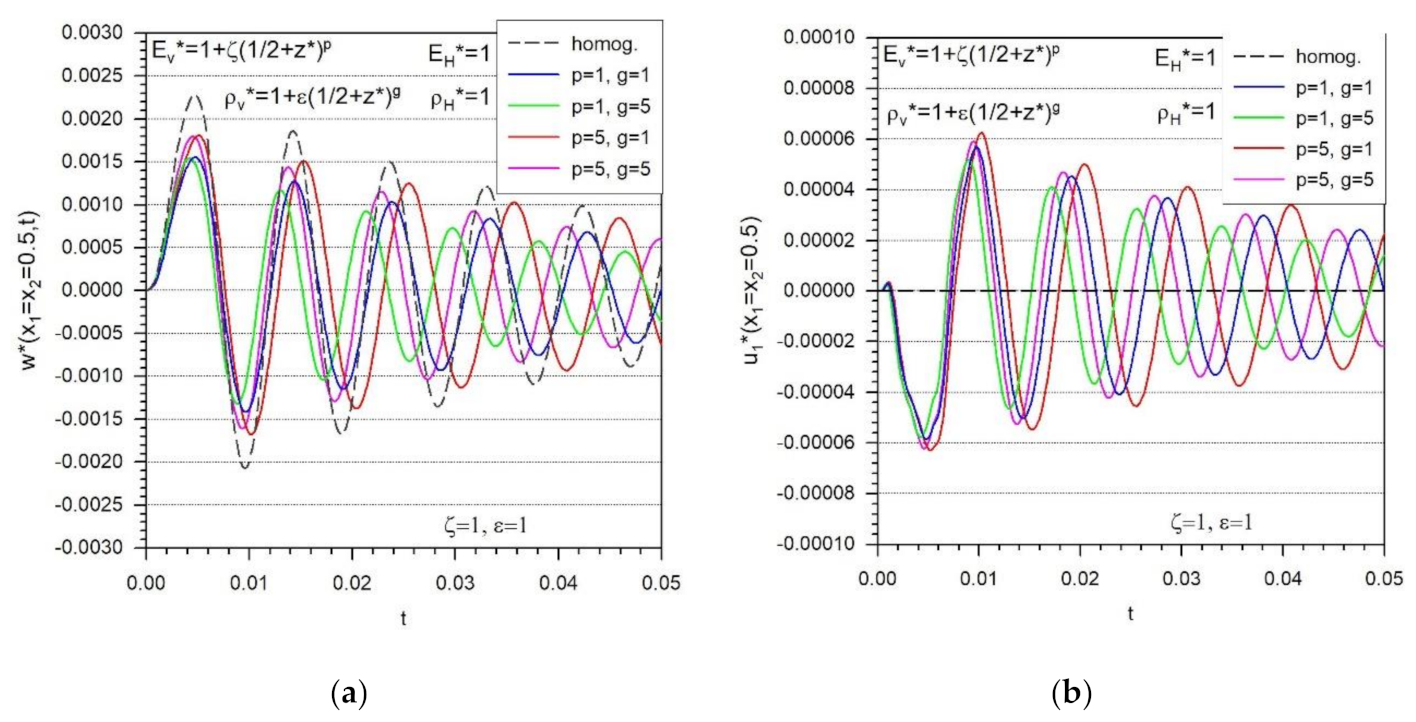
4.3. Response of FGM Plates under Transient Mechanical Loading

In this chapter, we shall present numerical experiments for the considered FGM plates with clamped edges, and transversally graded elastic modulus and mass density, subjected to Heaviside impact load. The initial conditions of IBVP are vanishing. Various combinations of the power law gradation exponents (p, g) and levels of gradation ( ε , ζ ) are considered. We consider also damping of the plate vibrations in view of the Rayleigh proportional damping model C = α M + β K [53], with choosing the parameters α = 0.001 and β = 0.0001 . To a numerical solution of the second-order ordinary differential equations (ODE) we apply the Newmark method [54] which is the implicit one-step time integration method.
Firstly, we shall present the time variation of central deflection and in-plane deformations for various combinations of gradations of the elastic modulus and mass density (Figure 8):
a.
Without gradation of material coefficients ( ε = 0 , ζ = 0 ).
b.
With transversal gradation of mass density only ( ε = 1 , ζ = 0 ).
c.
With transversal gradation of elastic modulus only ( ε = 0 , ζ = 1 ).
d.
With transversal gradation of elastic modulus and mass density ( ε = 1 , ζ = 1 ).
From Figure 8, one can see that both the amplitudes and frequencies of transversal deflection and the in-plane displacements are affected by the transversal gradation of the elastic modulus and/or mass density. The effect of the pure gradation of mass density on amplitudes is negligible as compared with the effect of the gradation of elastic modulus. However, the influence of each of the gradation coefficients ζ , ε on frequencies of vibrations is almost the same in magnitude but opposite in sign.
In what follows, we pay attention to the investigation of the role of higher values of the parameters ζ and ε and/or the gradation exponents p and g on the changes within the dynamic response of FGM plates with the transversal gradation of elastic modulus and mass density. From Figure 9 one can observe a significant influence of the level of gradation of each of the material coefficients on the frequencies of the vibrations of the central deflections and in-plane displacements. On the other hand, the amplitudes of vibrations are affected significantly only by the level of gradation of the elastic modulus. Since the frequency of oscillations is decreasing with the increasing value of ε and increases with the increasing value of ζ, one can tune the frequency rather sensitively by choosing the levels of gradations.
Figure 10 illustrates the study of the influence of the gradation exponents ( p , g ) on the dynamic response of the FGM plate. From Figure 10a we can see that the higher value of exponent p leads to a lower reduction in deflection, while the exponent g affected the frequency of vibrations remarkably, but the amplitudes are almost unaffected.

4.4. Response of FGM Plates under Transient Thermal Loading

The main focus of this chapter is on the investigation of the transient response of thermoelastic FGM plates subjected to thermal loadings defined as: θ ¯ * ( 0 , x 2 , x 3 , t ) = 0 , θ ¯ * ( 1 , x 2 , x 3 , t ) = 20 H ( t ) , q ¯ * ( x 1 , 0 , x 3 , t ) = 0 , q ¯ * ( x 1 , 1 , x 3 , t ) = 0 , q ¯ * ( x , ± h / 2 , t ) = 0 , θ ¯ * ( x , x 3 , t = 0 ) = 0 , where H ( t ) is standing for the Heaviside’s unit step function.
We shall present the results for temperature, in-plane deformation, and deflection fields for the case of pure transversal gradation of material coefficients. In Figure 11, it is illustrated that the transversal gradation of elastic modulus and/or thermal expansion coefficient has no influence on the time variation of temperature neither in the case of linear nor non-linear power law gradation. However, the power law gradation of material coefficients associated with heat conduction Equation (31), i.e., gradation parameters ω , χ , ε (the gradation levels for heat conduction coefficients, specific heat capacity, and mass density) results in remarkable changes in the time evolution of temperature fields. It is seen that the linear and/or non-linear case of gradation of the heat conduction coefficient accelerates the time evolution of temperature fields, while the gradation of the mass density and/or specific heat capacity decelerates the time evolution of temperature fields.
The time variation of in-plane displacements is presented in Figure 12. In contrast to the temperature fields, the in-plane displacements are clearly affected by the power law gradation of the thermal expansion coefficient ( α ); however, the impact of the gradation of elastic modulus ( E ) is negligible. The effect of the power law gradation of the heat conduction coefficients, specific heat capacity, and mass density on the time variation of in-plane displacements is similar to that on temperature fields.
From Figure 13. it is obvious that the power law gradation of elastic modulus and thermal expansion coefficient plays an important role in the deflection response of FGM thermoelastic plates subjected to transient thermal loadings. It can be seen that the transversal gradation of other material properties associated with the heat conduction equation has no influence on the deflection response of the FGM plate.

5. Conclusions

Three main conclusions can be drawn from the research presented in this paper:
(i)
The proposed unified formulation for plate bending problems allows:
  • A unique treatment of plate bending problems with simple switching among three plate bending theories (classical Kirchhoff–Love theory, first-order shear deformation theory, third-order shear deformation theory), differing in various deformation assumptions;
  • Physically correct derivation of governing equations and possible boundary conditions using variation principles;
  • To study the response of linear elastic plates with functionally graded material properties to static as well as dynamic mechanical and thermal loadings;
  • Comparison of results by three various theories using the same mathematical treatment.
(ii)
The developed advanced meshless method is characterized by:
  • Efficient solution of systems of partial differential equations with variable coefficients (due to functional gradation of material coefficients) with the same demands as in the case of homogeneous media;
  • Decomposition of the original fourth-order PDE to the system of the second-order PDE;
  • Enhanced accuracy of approximation of higher-order derivatives;
  • Improvement of computational efficiency by using the strong formulation;
  • Overcoming shortcomings of the standard finite element method with preserving its universality.
(iii)
A study of coupling effects by numerical simulations revealed:
  • The reliability (convergence and accuracy) and computational efficiency of developed numerical techniques;
  • The functional dependence of material coefficients gives rise to coupling effects among the field variables including the interaction between the in-plane deformation and bending modes;
  • To assess the influence of functional gradation parameters on the response of FGM plates to external loadings.
The proposed treatment of FGM plates could become a useful tool for designers because of the unified formulation including the assumptions of three various plate bending theories and owing to the wide, universal advanced numerical method for multi-physical plate bending problems.

Author Contributions

Conceptualization, V.S.; methodology, L.S. and V.S.; software, L.S.; formal analysis, L.S.; writing—original draft preparation, L.S.; writing—review and editing, V.S. and J.S.; supervision, J.S.; project administration, J.S. All authors have read and agreed to the published version of the manuscript.

Funding

The support provided by the Slovak Science and Technology Assistance Agency, registered under number APVV-18-0004, and Scientific Grant Agency of the Ministry of Education, Science, Research and Sport of the Slovak Republic and Slovak Academy of Sciences registered under number VEGA-2/0061/20.

Institutional Review Board Statement

Not applicable.

Informed Consent Statement

Not applicable.

Data Availability Statement

Not applicable.

Conflicts of Interest

The authors declare no conflict of interest. The funders had no role in the design of the study; in the collection, analyses, or interpretation of data; in the writing of the manuscript, or in the decision to publish the results.

References

  1. Kim, Y.; Park, J. A theory for the free vibration of a laminated composite rectangular plate with holes in aerospace applications. Compos. Struct. 2020, 251, 112571. [Google Scholar] [CrossRef]
  2. Prasad, K.R.; Syamsundar, C. Theoretical and FE analysis of epoxy composite pressure cylinder used for aerospace applications. Mater. Today Proc. 2019, 19, 1–9. [Google Scholar] [CrossRef]
  3. Krishnadasan, C.K.; Shanmugam, N.S.; Sivasubramonian, B.; Rao, B.N.; Suresh, R. Analytical studies and numerical predictions of stresses in shear joints of layered composite panels for aerospace applications. Compos. Struct. 2021, 255, 112927. [Google Scholar] [CrossRef]
  4. Nunes, J.P.; Silva, J.F. 5—Sandwiched composites in aerospace engineering. In Advanced Composite Materials for Aerospace Engineering; Rana, S., Fangueiro, R., Eds.; Woodhead Publishing: Cambridge, UK, 2016; pp. 129–174. [Google Scholar]
  5. Dhas, J.E.R.; Arun, M. A review on development of hybrid composites for aerospace applications. Mater. Today Proc. 2022, 64, 267–273. [Google Scholar] [CrossRef]
  6. Klemperer, C.J.; Maharaj, D. Composite electromagnetic interference shielding materials for aerospace applications. Compos. Struct. 2009, 91, 467–472. [Google Scholar] [CrossRef]
  7. Dai, H.-L.; Dai, T. Analysis for the thermoelastic bending of a functionally graded material cylindrical shell. Meccanica 2014, 49, 1069–1081. [Google Scholar] [CrossRef]
  8. Icardi, U.; Sola, F. Optimization of variable stiffness laminates and sandwiches undergoing impulsive dynamic loading. Aerospace 2015, 2, 602–626. [Google Scholar] [CrossRef]
  9. Sleight, D.W. Progressive Failure Analysis Methodology for Laminated Composite Structures; NASA/TP-1999-209107; NASA Center for AeroSpace Information (CASI): Hanover, MD, USA, 1999. [Google Scholar]
  10. Bezzie, Y.M.; Paramasivam, V.; Tilahun, S.; Selvaraj, S.K. A review on failure mechanisms and analysis of multidirectional laminates. Mater.-Today-Proc. 2021, 46, 7380–7388. [Google Scholar] [CrossRef]
  11. Hasan, M.Z. Interface failure of heated GLARETM fiber-metal laminates under bird strike. Aerospace 2020, 7, 28. [Google Scholar] [CrossRef]
  12. Wang, Y.Q.; Zu, J.W. Nonlinear dynamic thermoelastic response of rectangular FGM plates with longitudinal velocity. Compos. Part B Eng. 2017, 117, 74–88. [Google Scholar] [CrossRef]
  13. Jafarinezhad, M.R.; Eslami, M.R. Coupled thermoelasticity of FGM annular plate under lateral thermal shock. Compos. Struct. 2017, 168, 758–771. [Google Scholar] [CrossRef]
  14. Demirbas, M.D. Thermal stress analysis of functionally graded plates with temperature-dependent material properties using theory of elasticity. Compos. Part B Eng. 2017, 131, 100–124. [Google Scholar] [CrossRef]
  15. Yang, B.; Mei, J.; Chen, D.; Yu, F.; Yang, J. 3D thermo-mechanical solution of transversely isotropic and functionally graded graphene reinforced elliptical plates. Compos. Struct. 2018, 184, 1040–1048. [Google Scholar] [CrossRef]
  16. Reddy, J.N. Analysis of functionally graded plates. Int. J. Numer. Methods Eng. 2000, 47, 663–684. [Google Scholar] [CrossRef]
  17. Reddy, J.N.; Cheng, Z.Q. Three-dimensional thermomechanical deformations of functionally graded rectangular plates. Eur. J. Mech. Solids 2001, 20, 841–855. [Google Scholar] [CrossRef]
  18. Minh, P.P.; Manh, D.T.; Duc, N.D. Free vibration of cracked FGM plates with variable thickness resting on elastic foundations. Thin-Walled Struct. 2021, 161, 107425. [Google Scholar] [CrossRef]
  19. Adineh, M.; Kadkhodayan, M. Three-dimensional thermo-elastic analysis and dynamic response of a multi-directional functionally graded skew plate on elastic foundation. Compos. Part B Eng. 2017, 125, 227–240. [Google Scholar] [CrossRef]
  20. Yang, J.; Shen, H.S. Vibration characteristics and transient response of shear deformable functionally graded plates in thermal environments. J Sound Vib 2002, 255, 579–602. [Google Scholar] [CrossRef]
  21. Hashempoor, D.; Shojaeifard, M.H.; Talebitooti, R. Analytical modeling of functionally graded plates under general transversal loads. Proc. Rom. Acad. Ser. A 2013, 14, 309–316. [Google Scholar]
  22. Qin, S.; Wei, G.; Liu, Z.; Su, G. The elastic dynamics analysis of FGM using a meshless RRKPM. Eng. Anal. Bound. Elem. 2021, 129, 125–136. [Google Scholar] [CrossRef]
  23. Yang, J.; Shen, H.S. Non-linear analysis of functionally graded plates under transverse and in-plane loads. Int. J. Non-Linear Mech. 2003, 38, 467–482. [Google Scholar] [CrossRef]
  24. Daniel, I.M.; Ishai, O. Engineering Mechanics of Composite Materials; Oxford University Press: New York, NY, USA, 2006. [Google Scholar]
  25. Bhandari, M.; Purohit, K. Analysis of functionally graded material plate under transverse load for various boundary conditions. J. Mech. Civ. Eng. (IOSR-JMCE) 2014, 10, 46–55. [Google Scholar] [CrossRef]
  26. Ying, J.; Lu, C.; Lim, C.W. 3D thermoelasticity solutions for functionally graded thick plates. J. Zhejiang Univ. Sci. A 2009, 10, 327–336. [Google Scholar] [CrossRef]
  27. Ferreira, A.J.M.; Batra, R.C.; Roque, C.M.C.; Qian, L.F.; Martins, P.A.L.S. Static analysis of functionally graded plates using third order shear deformation theory and a meshless method. Compos. Struct 2005, 69, 449–457. [Google Scholar] [CrossRef]
  28. Suresh, S.; Mortensen, A. Fundamentals of Functionally Graded Materials, 1st ed.; IOM Communications: London, UK, 1998. [Google Scholar]
  29. Koizumi, M. FGM activities in Japan. Compos. Part B 1997, 28, 1–4. [Google Scholar] [CrossRef]
  30. Benveniste, Y. A new approach to the application of Mori–Tanaka’s theory in composite materials. Mech. Mater. 1987, 6, 147–157. [Google Scholar] [CrossRef]
  31. Mori, T.; Tanaka, T. Average stress in matrix and average elastic energy of materials with misfitting inclusions. Acta Met. 1973, 21, 571–574. [Google Scholar] [CrossRef]
  32. Hashin, Z.; Rosen, B.W. The elastic moduli of fiber-reinforced materials. ASME J. Appl. Mech. 1964, 4, 223–232. [Google Scholar] [CrossRef]
  33. Hashin, Z. Analysis of properties of fiber composites with anisotropic constituents. ASME J. Appl. Mech. 1979, 46, 543–550. [Google Scholar] [CrossRef]
  34. Chamis, C.C.; Sendeckyj, G.P. Critique on theories predicting thermoelastic properties of fibrous composites. J. Compos. Mater 1968, 3, 332–358. [Google Scholar] [CrossRef]
  35. Gibson, R.F. Principles of Composite Material Mechanics; McGraw-Hill: New York, NY, USA, 1994. [Google Scholar]
  36. Ardestani, M.M.; Soltani, B.; Shams, S. Analysis of functionally graded stiffened plates based on FSDT utilizing reproducing kernel particle method. Compos. Struct. 2014, 112, 231–240. [Google Scholar] [CrossRef]
  37. Vel, S.S.; Batra, R.C. Exact solution for thermoelastic deformations of functionally graded thick rectangular plates. AIAAJ 2002, 40, 1421–1433. [Google Scholar] [CrossRef]
  38. Reddy, J.N.; Wang, C.M.; Kitipornchai, S. Axisymmetric bending of functionally graded circular and annular plates. Eur. J. Mech. A/Solids 1999, 18, 185–199. [Google Scholar] [CrossRef]
  39. Xu, Y.; Zhou, D. Three-dimensional elasticity solution of functionally graded rectangular plates with variable thickness. Compos. Struct. 2009, 91, 56–65. [Google Scholar] [CrossRef]
  40. Atluri, S.N. The Meshless Method, (MLPG) For Domain & BIE Discretizations; Tech Science Press: Encino, CA, USA, 2004. [Google Scholar]
  41. Krysl, P.; Belytschko, T. Analysis of thin plates by the element-free Galerkin method. Comput. Mech. 1995, 17, 26–35. [Google Scholar] [CrossRef]
  42. Lu, Y.Y.; Belytschko, T.; Gu, L. A new implementation of the element free Galerkin method. Comp. Meth. Appl. Mech. Eng. 1994, 113, 397–414. [Google Scholar] [CrossRef]
  43. Lancaster, P.; Salkauskas, K. Surfaces generated by moving least square method. Math. Comput. 1981, 37, 141–158. [Google Scholar] [CrossRef]
  44. Sladek, V.; Sladek, J.; Zhang, C. Computation of stresses in non-homogeneous elastic solids by local integral equation method: A comparative study. Comput. Mech. 2008, 41, 827–845. [Google Scholar] [CrossRef]
  45. Sladek, V.; Sladek, J.; Zhang, C. Local integral equation formulation for axially symmetric problems involving elastic FGM. Eng. Anal. Bound. Elem. 2008, 32, 1012–1024. [Google Scholar] [CrossRef]
  46. Sladek, V.; Sladek, J. Local integral equations implemented by MLS approximation and analytical integrations. Eng. Anal. Bound. Elem. 2010, 34, 904–913. [Google Scholar] [CrossRef]
  47. Sladek, V.; Sladek, J.; Sator, L. Physical decomposition of thin plate bending problems and their solution by mesh-free methods. Eng. Anal. Bound. Elem. 2013, 37, 348–365. [Google Scholar] [CrossRef]
  48. Sator, L.; Sladek, V.; Sladek, J. Elastodynamics of FGM plates by meshfree method. Compos. Struct 2016, 40, 100–110. [Google Scholar]
  49. Sator, L.; Sladek, V.; Sladek, J. Coupling effects in elastic analysis of FGM plates under thermal load: Classical thermoelasticitz analysis by a meshless methods. Compos. Part B 2018, 146, 176–188. [Google Scholar] [CrossRef]
  50. Sator, L.; Sladek, V.; Sladek, J. Bending of FGM composite plates by mesh-free methods. Compos. Struct 2014, 115, 309–322. [Google Scholar] [CrossRef]
  51. Timoshenko, S.P.; Woinowsky-Krieger, S. Theory of Plates and Shells; McGraw-Hill: New York, NY, USA, 1959. [Google Scholar]
  52. Sladek, V.; Sladek, J.; Zhang, C. On increasing computational efficiency of local integral equation method combined with meshless implementations. CMES 2010, 63, 243–263. [Google Scholar]
  53. Liu, M.; Gorman, D.G. Formulation of Rayleigh damping and its extensions. Comput. Struct. 1995, 57, 277–285. [Google Scholar] [CrossRef]
  54. Hashamdar, H.; Ibrahim, Z.; Jameel, M. Finite element analysis of nonlinear structures with Newmark method. Int. J. Phys. Sci. 2011, 6, 61395–61403. [Google Scholar]
Figure 1. Sketch of a square plate.
Aerospace 09 00425 g001
Figure 2. Dimensionless deflections of homogeneous and/or FGM square plates with various parameters of gradation of Young modulus.
Aerospace 09 00425 g002
Figure 3. (a) Comparison of convergence rates in the homogeneous elastic plate; (b) computational efficiency of proposed meshless method for both the differentiation techniques.
Aerospace 09 00425 g003aAerospace 09 00425 g003b
Figure 4. Three-dimensional map of deflections for (a) homogeneous plate and (b) transversally graded FGM plate with gradation parameters ζ = 1, p = 1.
Aerospace 09 00425 g004
Figure 5. Three-dimensional map of in-plane deformations for (a) homogeneous plate and (b) transversally graded FGM plate with gradation parameters ζ = 1, p = 1.
Aerospace 09 00425 g005
Figure 6. (a) Deflections and (b) in-plane deformations in homogeneous as well as FGM plates.
Aerospace 09 00425 g006
Figure 7. Dependence of the reduction of maximal deflections on (a) parameter ζ and (b) on exponent p.
Aerospace 09 00425 g007
Figure 8. Comparison of influences of the various combinations of the level of gradation of the mass density (ε) and/or the elastic modulus (ζ) on the time variation of: (a) the dimensionless central deflection, (b) the dimensionless in-plane deformation.
Aerospace 09 00425 g008
Figure 9. Effect of the level of gradation of the mass density (ε) and/or the elastic modulus (ζ) on the time variation of: (a) the dimensionless central deflection, (b) the dimensionless in-plane deformation.
Aerospace 09 00425 g009
Figure 10. Influences of the gradation exponent of the mass density (g) and/or the elastic modulus (p) on the time variation of: (a) the dimensionless central deflection, (b) the dimensionless in-plane deformation.
Aerospace 09 00425 g010
Figure 11. Time variation of the temperature in the homogeneous as well as FGM plates.
Aerospace 09 00425 g011
Figure 12. Time variation of the in-plane displacements in homogeneous as well as FGM plates.
Aerospace 09 00425 g012
Figure 13. Time variations of the deflections in homogeneous as well as FGM plates.
Aerospace 09 00425 g013
Publisher’s Note: MDPI stays neutral with regard to jurisdictional claims in published maps and institutional affiliations.

