Shape Optimisation of Assembled Plate Structures with the Boundary Element Method

Abstract

A novel methodology is presented for performing sensitivity analyses of assembled plate structures using the Boundary Element Method (BEM). The main novelty of this work is that the exact implicit derivatives of the BEM formulations for assembled plate structures have been derived for the first time and incorporated into a newly developed Implicit Differentiation Method (IDM), enabling sensitivity analyses to be conducted for more complex and realistic structures in a more accurate, robust, and efficient manner than previous approaches. Three numerical examples are investigated to validate the derived exact implicit derivatives and to demonstrate how they could be used for a potential application involving the shape optimisation of a complex X-core structure from the canard of a Eurofighter Typhoon fighter jet. Results show that the newly developed IDM is more accurate, robust, and efficient when compared to alternative methodologies using derivatives obtained from methods such as the Finite Difference Method (FDM) and the Finite Element Method (FEM).

1. Introduction

Sensitivity analysis plays a key role in the design of structures. It is very important for engineers to understand the sensitivity of a structure’s performance to changes in geometrical, material, or loading parameters. Sensitivity analysis also enables engineers to optimise the design of their structures and maximise their safety.

The Boundary Element Method (BEM) is a very useful tool for conducting sensitivity analyses of structures. When modelling a structure, the BEM only requires the outer boundary of the structure to be discretised into elements. This makes the BEM a very efficient tool for sensitivity analyses, because only a relatively small part of the model needs to be re-meshed during the analyses. Furthermore, the BEM can often achieve a similar level accuracy to the Finite Element Method (FEM) while using a courser mesh with fewer elements, indicating that the BEM would be a very efficient method for optimisation problems involving the calculation of many sensitivities over many iterations [1].

Most prior work on structural sensitivity analysis with the BEM amongst the research community has involved 2D structures [2,3,4,5,6,7,8,9,10,11], and 3D structures [12,13,14,15,16,17] to a smaller degree. There have only been a few prior research works on the topic of structural sensitivity analysis with the BEM that have involved plate structures, with some examples being [18,19]. There are many structures in engineering, particularly in aircraft, that are not able to be modelled accurately in 2D. Furthermore, although modelling a structure in 3D can lead to very accurate results, it is often more computationally efficient to model it as a plate structure, without a noticeable loss in modelling accuracy. Previous works on plate structural sensitivity analysis with the BEM [18,19] have only considered simple single-plate structures, which have a limited range of application. Assembled-plate structures, on the other hand, have a much greater range of application and enable more complex plate structures to be investigated. However, there are several challenges associated with the sensitivity analysis of assembled structures—there are significantly more geometric parameters involved compared to single-plate structures and the interaction between these parameters is more complex, increasing the computation time and complexity. The BEM, due to its inherent advantages described earlier, would be very effective at addressing these challenges. Therefore, this current work aims to build upon previous work by the research community and develop a novel methodology for conducting sensitivity analyses for assembled-plate structures—enabling complex plate structures to be investigated both accurately and efficiently.

A common approach to calculating sensitivities is with the Finite Difference Method (FDM). The FDM is a relatively simple method that uses finite differences to calculate sensitivities. Although simple to implement, a drawback of the FDM is that its accuracy is highly dependent on the step-size used. An alternative approach to the FDM would be to derive the exact implicit derivatives of the BEM formulations. This Implicit Differentiation Method (IDM), since it uses the exact derivatives, would be more accurate and robust than the FDM. In addition, by exploiting the inherent advantages of the BEM mentioned earlier, it would also be more computationally efficient, since large parts of the BEM mesh would remain unchanged during the sensitivity analyses. Previous examples of work by the research community involving the derivation of the exact implicit derivatives of BEM formulations include [2,20,21,22] for 2D structures, [23] for 3D structures, and [18,19] for simple single-plate structures. There have not yet been any works involving assembled-plate structures.

In summary, the main novelty of this current work is that the exact implicit derivatives of the BEM assembled-plate structure formulations have been derived for the first time. Previous works have only derived these derivatives for simple single-plate structures. By deriving the derivatives for assembled plate structures, a wider range of more realistic and complex structures can be investigated. The use of these derivatives, along with the inherent advantages of the BEM, can significantly improve the accuracy, robustness, and computational efficiency when performing structural sensitivity analyses of these more realistic and complex structures. Potential applications of this newly developed methodology include the shape optimisation or structural reliability analysis of complex plate structures.

The formulations behind the BEM for assembled plate structures, as well as the exact implicit derivatives of these formulations, are presented in Section 2. Several numerical examples are presented in Section 3 to validate the derived exact implicit derivatives and to demonstrate their accuracy, robustness, and efficiency. A numerical example involving the shape optimisation of a complex assembled plate structure is also presented to demonstrate a potential application of the derived exact implicit derivatives.

2. Methodology

In this section, the formulations of the Boundary Element Method (BEM) and the Implicit Differentiation Method (IDM) for assembled plate structures are presented. In this work, Latin letter indexes (e.g., i, j, k) can take values from 1 to 3, whereas Greek letter indexes (e.g., $\alpha$, $\beta$, $\rho$, $\gamma$) can take values of either 1 or 2.

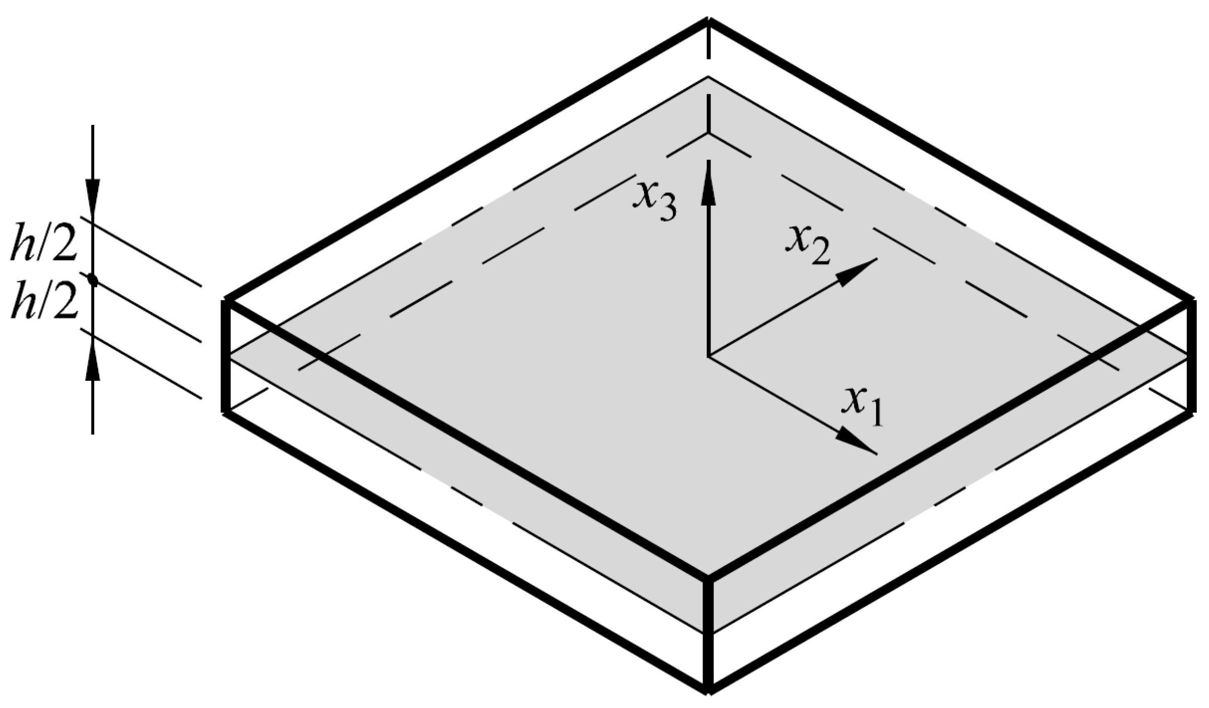
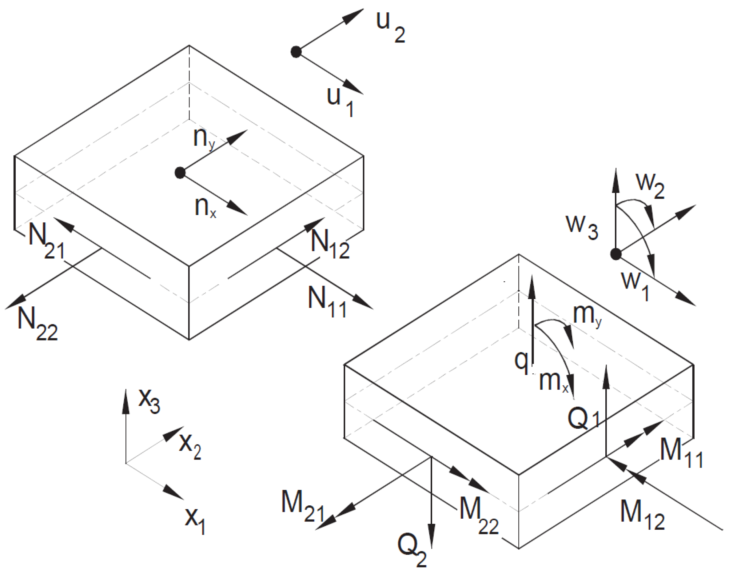
2.1. Plate Theory Notation in the Boundary Element Method

Figure 1 shows a plate of thickness h ($-h/2\le x_3\le +h/2$). The membrane of the plate is the $x_1-x_2$ plane.

The sign convections for the displacements, rotations, tractions, and moments for plates is shown in Figure 2.

The in-plane displacements of the plate are given in Equation (1):

$$\mathbf{u}=\left[\begin{array}{c}{u}_1\\ u_2\end{array}\right]$$

(1)

The rotations and out-of-plane displacement of the plate are given in Equation (2):

$$\mathbf{w}=\left[\begin{array}{c}{w}_1\\ w_2\\ w_3\end{array}\right]$$

(2)

where $w_1$ and $w_2$ are rotations, and $w_3$ is the out-of-plane displacement of the plate in direction $x_3$.

The membrane tractions are given in Equation (3):

$$\mathbf{t}=\left[\begin{array}{c}{t}_1\\ t_2\end{array}\right]=\left[\begin{array}{c}{N}_{11}{n}_1+N_{12}{n}_2\\ N_{21}{n}_1+N_{22}{n}_2\end{array}\right]$$

(3)

where $N_{\alpha \beta }$ are the membrane stress resultants, and $n_{\beta }$ are the components of the outward normal vector of the boundary of the plate.

The bending and shear tractions are given in Equation (4):

$$\mathbf{p}=\left[\begin{array}{c}{p}_1\\ p_2\\ p_3\end{array}\right]\left[\begin{array}{c}{p}_1\\ p_2\end{array}\right]=\left[\begin{array}{c}{M}_{11}{n}_1+N_{12}{n}_2\\ M_{21}{n}_1+N_{22}{n}_2\end{array}\right]p_3=Q_1{n}_1+Q_2{n}_2$$

(4)

where $M_{\alpha \beta }$ are the bending stress resultants, and $Q_{\alpha }$ are the shear stress resultants.

2.2. The Boundary Element Method for Plate Structures

In the approach developed by Dirgantara and Aliabadi [24], the Boundary Element Method (BEM) for plate structures involves using the Reissner theory to model the bending and shear behaviour of plates, whereas 2D plane stress theory is used to model the behaviour of the membrane of plates. The BEM equation for the plate membrane is given in Equation (5):

$$\begin{array}{cc}\hfill {\mathbf{C}}^m\mathbf{u}& +\sum _{n_e=1}^{N_e}\left({\int }_{{\Gamma }_{n_e}}{\mathbf{T}}^m{\mathit{\psi }}_e^{\mathrm{T}}\mathbf{d}{\Gamma }_{n_e}\right){\mathbf{u}}^{n_e}=\sum _{n_e=1}^{N_e}\left({\int }_{{\Gamma }_{n_e}}{\mathbf{U}}^m{\mathit{\psi }}_e^{\mathrm{T}}\mathbf{d}{\Gamma }_{n_e}\right){\mathbf{t}}^{n_e}\hfill \end{array}$$

(5)

The BEM equation for bending and shear is given in Equation (6):

$$\begin{array}{cc}\hfill {\mathbf{C}}^b\mathbf{w}& +\sum _{n_e=1}^{N_e}\left({\int }_{{\Gamma }_{n_e}}{\mathbf{T}}^b{\mathit{\psi }}_e^{\mathrm{T}}\mathbf{d}{\Gamma }_{n_e}\right){\mathbf{w}}^{n_e}=\sum _{n_e=1}^{N_e}\left({\int }_{{\Gamma }_{n_e}}{\mathbf{U}}^b{\mathit{\psi }}_e^{\mathrm{T}}\mathbf{d}{\Gamma }_{n_e}\right){\mathbf{p}}^{n_e}+q_3\sum _{n_e=1}^{N_e}\left({\int }_{{\Gamma }_{n_e}}{\mathbf{B}}^b\mathbf{d}{\Gamma }_{n_e}\right)\hfill \end{array}$$

(6)

$N_e$ denotes the number of elements on the external boundary. ${\mathbf{T}}^m$, ${\mathbf{T}}^b$, ${\mathbf{U}}^m$,${\mathbf{U}}^b$, and ${\mathbf{B}}^b$ are fundamental solutions evaluated along the surface of element $n_e$, ${\Gamma }_{n_e}$. $q_3$ is a uniform load applied over the surface of the plate. The terms ${\mathbf{C}}^m$ and ${\mathbf{C}}^b$ are free terms and their values can be directly evaluated from a consideration of rigid body motion [1]. Quadratic boundary elements, consisting of three nodes and ten Gaussian quadrature integration points, were used in this work. ${\mathit{\psi }}_e^{\mathrm{T}}$ contains the continuous shape functions for the quadratic boundary elements. More information on the numerical integration approach used in this work can be found in [1]. Detailed forms of the above equations can be found in [1,19,22,24].

${\mathbf{u}}^{n_e}$ is a $(2\times 1)$ vector that contains the in-plane displacements for element $n_e$ and is shown in Equation (7):

$${\mathbf{u}}^{n_e}=\left[\begin{array}{c}{u}_1^{n_e}\\ u_2^{n_e}\end{array}\right]$$

(7)

${\mathbf{w}}^{n_e}$ is a $(3\times 1)$ vector that contains rotations $w_1$ and $w_2$, and vertical displacement $w_3$ for element $n_e$ and is shown in Equation (8):

$${\mathbf{w}}^{n_e}=\left[\begin{array}{c}{w}_1^{n_e}\\ w_2^{n_e}\\ w_3^{n_e}\end{array}\right]$$

(8)

${\mathbf{t}}^{n_e}$ is a $(2\times 1)$ vector that contains the tractions due to membrane stress resultants for element $n_e$ and is shown in Equation (9):

$${\mathbf{t}}^{n_e}=\left[\begin{array}{c}{t}_1^{n_e}\\ t_2^{n_e}\end{array}\right]$$

(9)

${\mathbf{p}}^{n_e}$ is a $(3\times 1)$ vector that contains bending tractions $p_1$ and $p_2$, and shear traction $p_3$ for element $n_e$ and is shown in Equation (10):

$${\mathbf{p}}^{n_e}=\left[\begin{array}{c}{p}_1^{n_e}\\ p_2^{n_e}\\ p_3^{n_e}\end{array}\right]$$

(10)

By using the above equations, the system of equations shown in Equation (11) can be created:

$$\mathbf{Hu}=\mathbf{Gt}$$

(11)

where $\mathbf{u}$ contains displacements and rotations, and $\mathbf{t}$ contains membrane, bending, and shear tractions. $\mathbf{G}$ and $\mathbf{H}$ are matrices of coefficients. This system can be rewritten as shown in Equation (12):

$$\mathbf{AX}=\mathbf{F}$$

(12)

where $\mathbf{X}$ contains all of the unknown displacements, rotations, and tractions. $\mathbf{A}$ is a matrix that contains the coefficients from $\mathbf{H}$ and $\mathbf{G}$. $\mathbf{F}$ contains the known displacements, rotations, and tractions multiplied by the corresponding coefficients from $\mathbf{H}$ and $\mathbf{G}$. Details of this procedure are shown in [22].

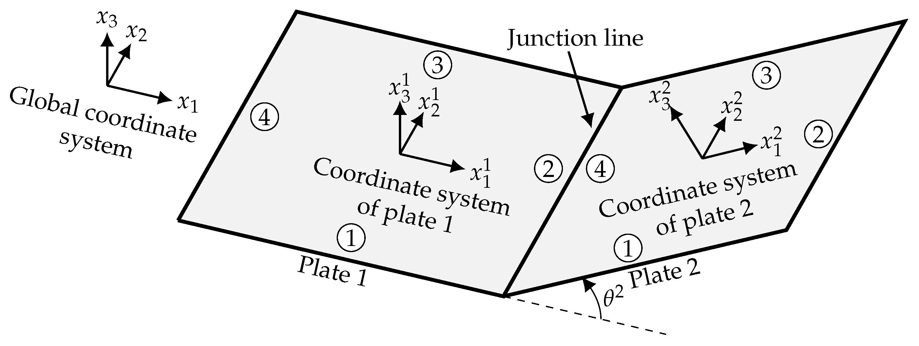
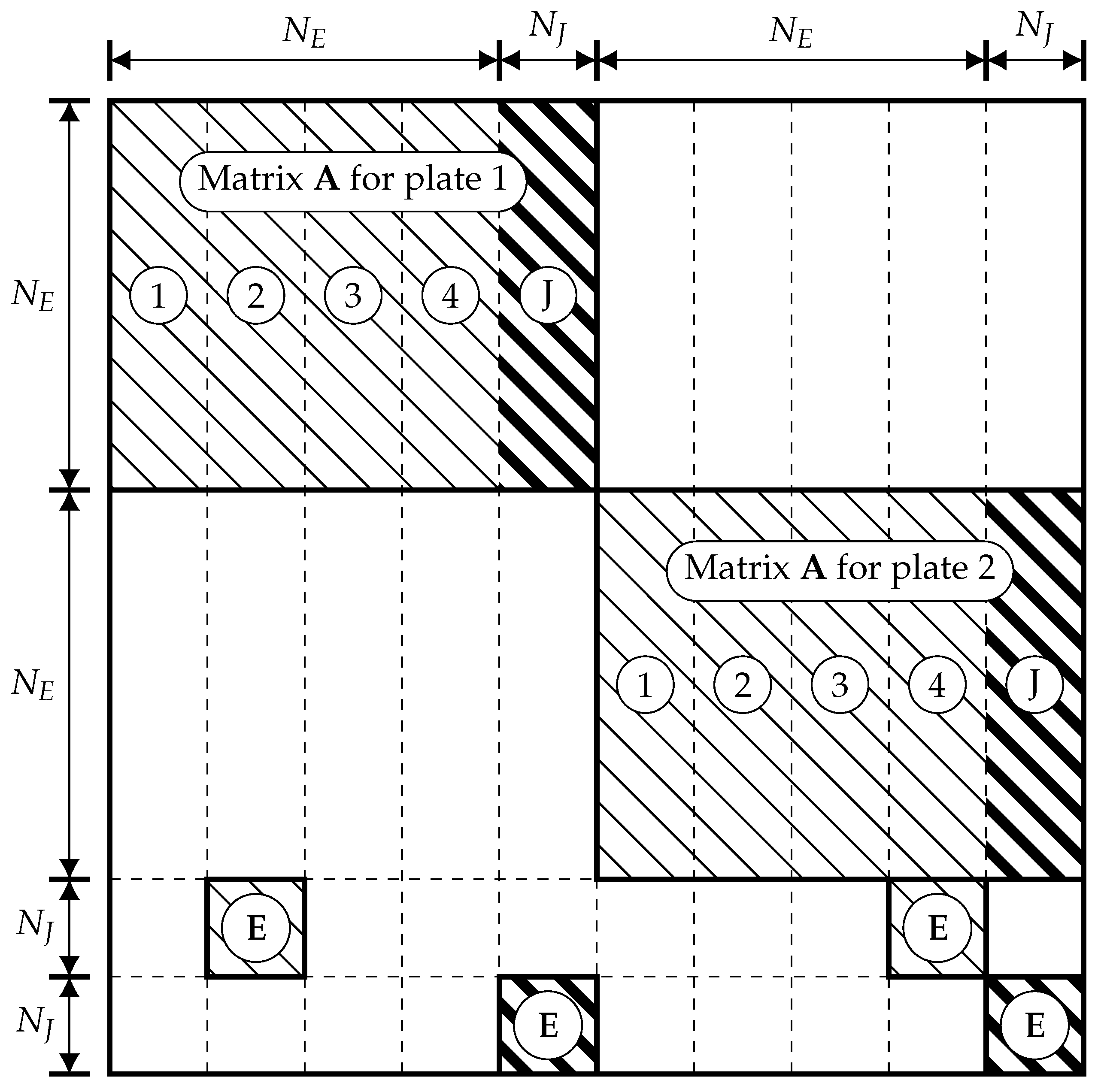
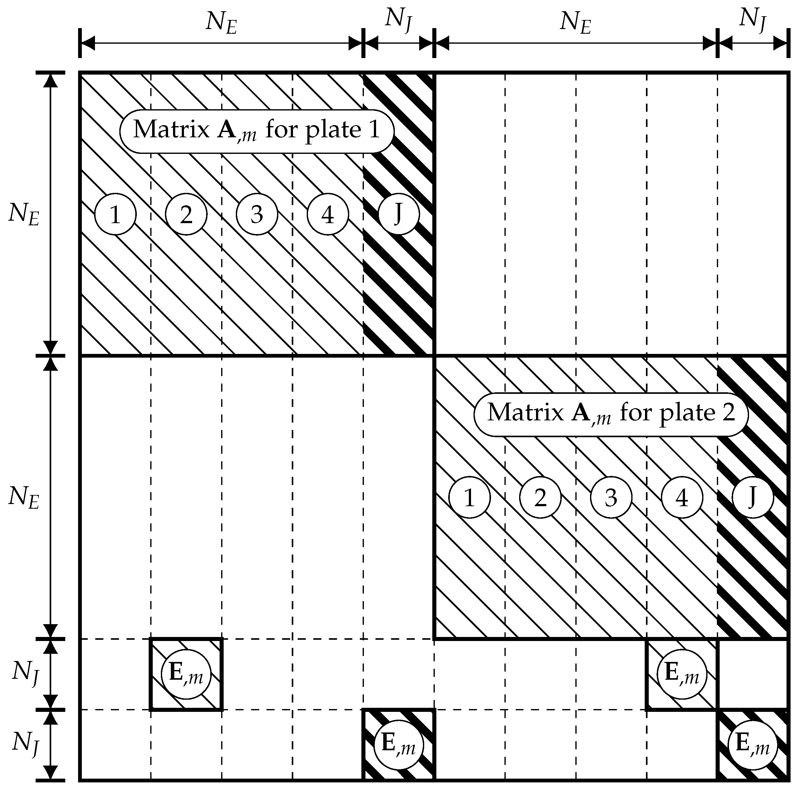
2.3. The Boundary Element Method for Assembled Plate Structures

The above procedure is straightforward for a structure consisting of a single plate. However, the range of application for a structure consisting of a single plate is very limited. To widen the range of application of the above procedure, it must be extended to structures consisting of multiple plates joined together. This would significantly expand the range of application of the above procedure and enable more complex structures, including many structures found in aircraft, to be investigated in an accurate, robust, and computationally efficient manner.

An example of an assembled plate structure consisting of two plates is shown in Figure 3. Each plate has its own local coordinate system, which is used when calculating the matrix $\mathbf{A}$ of each plate. The plates are connected along a junction line.

The $\mathbf{A}$ matrix of the assembled plate structure in Figure 3 is shown in Figure 4. The parts of the $\mathbf{A}$ matrices corresponding to the edges 1–4 are shown. To account for the connection between the two plates at the junction line, additional columns are added to the $\mathbf{A}$ matrix of each plate, and are labelled as ‘J’. The number of elements on the boundary of each plate is assumed to be equal, and is $N_E$. The number of elements along the junction line is $N_J$. The equilibrium equations, which describe the relationships between the displacements and tractions of the connected plates, can be found in the matrices labelled $\mathbf{E}$.

For an assembled plate structure, the plates are joined together by junction lines, as shown in Figure 3. The junction line is along the $x_2$-axis. Each plate has its own local set of coordinates ($x_1^i,x_2^i,x_3^i$) with $i=1,2,\dots ,N$, where N is the number of plates. To account for the fact that neighbouring plates will influence one another in terms of displacements and tractions, equilibrium equations must be derived along junction lines. These equilibrium equations are used in the matrices labelled $\mathbf{E}$ in Figure 4.

The displacement equilibrium equations are shown in Equations (13)–(17):

$$u_1^{1}cos\left({\theta }^1\right)-w_3^{1}sin\left({\theta }^1\right)=u_1^{2}cos\left({\theta }^2\right)-w_3^{2}sin\left({\theta }^2\right)=\dots =u_1^{N}cos\left({\theta }^N\right)-w_3^{N}sin\left({\theta }^N\right)$$

(13)

$$u_1^{1}sin\left({\theta }^1\right)+w_3^{1}cos\left({\theta }^1\right)=u_1^{2}sin\left({\theta }^2\right)+w_3^{2}cos\left({\theta }^2\right)=\dots =u_1^{N}sin\left({\theta }^N\right)+w_3^{N}cos\left({\theta }^N\right)$$

(14)

$$u_2^1=u_2^2=\dots =u_2^N$$

(15)

$$w_1^1=w_1^2=\dots =w_1^N$$

(16)

$$w_2^1=w_2^2=\dots =w_2^N=0$$

(17)

The traction equilibrium equations are shown in Equations (18)–(21):

$$\sum _{i=1}^N\left(t_1^{i}cos\left({\theta }^i\right)-p_3^{i}sin\left({\theta }^i\right)\right)=0$$

(18)

$$\sum _{i=1}^N\left(t_1^{i}sin\left({\theta }^i\right)+p_3^{i}cos\left({\theta }^i\right)\right)=0$$

(19)

$$\sum _{i=1}^N{t}_2^i=0$$

(20)

$$\sum _{i=1}^N{p}_{\alpha }^i=0$$

(21)

where ${\theta }^i$ is the angle of the local coordinate axis $x_1^i$ of the i’th plate to the global coordinate axis $x_1$, and $u_1^i$ is the displacement in the local coordinate axis $x_1^i$ of the i’th plate, etc. In the equilibrium equations shown above, it is assumed that there is no offset between the membranes of the joined plates. The equations in the case where is there an offset can be found in [1].

2.4. The Implicit Differentiation Method for Plate Structures

In the Implicit Differentiation Method (IDM), the derivatives of Equations (5) and (6) can be calculated with respect to a geometric parameter $Z_m$ (such as the length or width of a plate), or with respect to the thickness of the plate h.

The derivative of Equation (5) with respect to $Z_m$ is shown in Equation (22):

$$\begin{array}{cc}\hfill {\mathbf{C}}^m{\mathbf{u}}_{,m}& +\sum _{n_e=1}^{N_e}\left({\int }_{{\Gamma }_{n_e}}{\mathbf{T}}_{,m}^m{\mathit{\psi }}_e^{\mathrm{T}}\mathbf{d}{\Gamma }_{n_e}+{\int }_{{\Gamma }_{n_e}}{\mathbf{T}}^m{\mathit{\psi }}_e^{\mathrm{T}}{\left(\mathbf{d}{\Gamma }_{n_e}\right)}_{,m}\right){\mathbf{u}}^{n_e}\hfill \\ \hfill & +\sum _{n_e=1}^{N_e}\left({\int }_{{\Gamma }_{n_e}}{\mathbf{T}}^m{\mathit{\psi }}_e^{\mathrm{T}}\mathbf{d}{\Gamma }_{n_e}\right){\mathbf{u}}_{,m}^{n_e}\hfill \\ \hfill & =\sum _{n_e=1}^{N_e}\left({\int }_{{\Gamma }_{n_e}}{\mathbf{U}}_{,m}^m{\mathit{\psi }}_e^{\mathrm{T}}\mathbf{d}{\Gamma }_{n_e}+{\int }_{{\Gamma }_{n_e}}{\mathbf{U}}^m{\mathit{\psi }}_e^{\mathrm{T}}{\left(\mathbf{d}{\Gamma }_{n_e}\right)}_{,m}\right){\mathbf{t}}^{n_e}\hfill \\ \hfill & +\sum _{n_e=1}^{N_e}\left({\int }_{{\Gamma }_{n_e}}{\mathbf{U}}^m{\mathit{\psi }}_e^{\mathrm{T}}\mathbf{d}{\Gamma }_{n_e}\right){\mathbf{t}}_{,m}^{n_e}\hfill \end{array}$$

(22)

The derivative of Equation (5) with respect to h is shown in Equation (23):

$$\begin{array}{cc}\hfill {\mathbf{C}}^m{\mathbf{u}}_{,h}& +\sum _{n_e=1}^{N_e}\left({\int }_{{\Gamma }_{n_e}}{\mathbf{T}}_{,h}^m{\mathit{\psi }}_e^{\mathrm{T}}\mathbf{d}{\Gamma }_{n_e}+{\int }_{{\Gamma }_{n_e}}{\mathbf{T}}^m{\mathit{\psi }}_e^{\mathrm{T}}{\left(\mathbf{d}{\Gamma }_{n_e}\right)}_{,h}\right){\mathbf{u}}^{n_e}\hfill \\ \hfill & +\sum _{n_e=1}^{N_e}\left({\int }_{{\Gamma }_{n_e}}{\mathbf{T}}^m{\mathit{\psi }}_e^{\mathrm{T}}\mathbf{d}{\Gamma }_{n_e}\right){\mathbf{u}}_{,h}^{n_e}\hfill \\ \hfill & =\sum _{n_e=1}^{N_e}\left({\int }_{{\Gamma }_{n_e}}{\mathbf{U}}_{,h}^m{\mathit{\psi }}_e^{\mathrm{T}}\mathbf{d}{\Gamma }_{n_e}+{\int }_{{\Gamma }_{n_e}}{\mathbf{U}}^m{\mathit{\psi }}_e^{\mathrm{T}}{\left(\mathbf{d}{\Gamma }_{n_e}\right)}_{,h}\right){\mathbf{t}}^{n_e}\hfill \\ \hfill & +\sum _{n_e=1}^{N_e}\left({\int }_{{\Gamma }_{n_e}}{\mathbf{U}}^m{\mathit{\psi }}_e^{\mathrm{T}}\mathbf{d}{\Gamma }_{n_e}\right){\mathbf{t}}_{,h}^{n_e}\hfill \end{array}$$

(23)

The derivative of Equation (6) with respect to $Z_m$ is shown in Equation (24):

$$\begin{array}{cc}\hfill {\mathbf{C}}^b{\mathbf{w}}_{,m}& +\sum _{n_e=1}^{N_e}\left({\int }_{{\Gamma }_{n_e}}{\mathbf{T}}_{,m}^b{\mathit{\psi }}_e^{\mathrm{T}}\mathbf{d}{\Gamma }_{n_e}+{\int }_{{\Gamma }_{n_e}}{\mathbf{T}}^b{\mathit{\psi }}_e^{\mathrm{T}}{\left(\mathbf{d}{\Gamma }_{n_e}\right)}_{,m}\right){\mathbf{w}}^{n_e}\hfill \\ \hfill & +\sum _{n_e=1}^{N_e}\left({\int }_{{\Gamma }_{n_e}}{\mathbf{T}}^b{\mathit{\psi }}_e^{\mathrm{T}}\mathbf{d}{\Gamma }_{n_e}\right){\mathbf{w}}_{,m}^{n_e}\hfill \\ \hfill & =\sum _{n_e=1}^{N_e}\left({\int }_{{\Gamma }_{n_e}}{\mathbf{U}}_{,m}^b{\mathit{\psi }}_e^{\mathrm{T}}\mathbf{d}{\Gamma }_{n_e}+{\int }_{{\Gamma }_{n_e}}{\mathbf{U}}^b{\mathit{\psi }}_e^{\mathrm{T}}{\left(\mathbf{d}{\Gamma }_{n_e}\right)}_{,m}\right){\mathbf{p}}^{n_e}\hfill \\ \hfill & +\sum _{n_e=1}^{N_e}\left({\int }_{{\Gamma }_{n_e}}{\mathbf{U}}^b{\mathit{\psi }}_e^{\mathrm{T}}\mathbf{d}{\Gamma }_{n_e}\right){\mathbf{p}}_{,m}^{n_e}\hfill \\ \hfill & +q_3\sum _{n_e=1}^{N_e}\left({\int }_{{\Gamma }_{n_e}}{\mathbf{B}}_{,m}^b\mathbf{d}{\Gamma }_{n_e}+{\int }_{{\Gamma }_{n_e}}{\mathbf{B}}^b{\left(\mathbf{d}{\Gamma }_{n_e}\right)}_{,m}\right)\hfill \end{array}$$

(24)

The derivative of Equation (6) with respect to h is shown in Equation (25):

$$\begin{array}{cc}\hfill {\mathbf{C}}^b{\mathbf{w}}_{,h}& +\sum _{n_e=1}^{N_e}\left({\int }_{{\Gamma }_{n_e}}{\mathbf{T}}_{,h}^b{\mathit{\psi }}_e^{\mathrm{T}}\mathbf{d}{\Gamma }_{n_e}+{\int }_{{\Gamma }_{n_e}}{\mathbf{T}}^b{\mathit{\psi }}_e^{\mathrm{T}}{\left(\mathbf{d}{\Gamma }_{n_e}\right)}_{,h}\right){\mathbf{w}}^{n_e}\hfill \\ \hfill & +\sum _{n_e=1}^{N_e}\left({\int }_{{\Gamma }_{n_e}}{\mathbf{T}}^b{\mathit{\psi }}_e^{\mathrm{T}}\mathbf{d}{\Gamma }_{n_e}\right){\mathbf{w}}_{,h}^{n_e}\hfill \\ \hfill & =\sum _{n_e=1}^{N_e}\left({\int }_{{\Gamma }_{n_e}}{\mathbf{U}}_{,h}^b{\mathit{\psi }}_e^{\mathrm{T}}\mathbf{d}{\Gamma }_{n_e}+{\int }_{{\Gamma }_{n_e}}{\mathbf{U}}^b{\mathit{\psi }}_e^{\mathrm{T}}{\left(\mathbf{d}{\Gamma }_{n_e}\right)}_{,h}\right){\mathbf{p}}^{n_e}\hfill \\ \hfill & +\sum _{n_e=1}^{N_e}\left({\int }_{{\Gamma }_{n_e}}{\mathbf{U}}^b{\mathit{\psi }}_e^{\mathrm{T}}\mathbf{d}{\Gamma }_{n_e}\right){\mathbf{p}}_{,h}^{n_e}\hfill \\ \hfill & +q_3\sum _{n_e=1}^{N_e}\left({\int }_{{\Gamma }_{n_e}}{\mathbf{B}}_{,h}^b\mathbf{d}{\Gamma }_{n_e}+{\int }_{{\Gamma }_{n_e}}{\mathbf{B}}^b{\left(\mathbf{d}{\Gamma }_{n_e}\right)}_{,h}\right)\hfill \end{array}$$

(25)

In the above equations, ${\mathbf{T}}_{,m}^m$, ${\mathbf{T}}_{,m}^b$, ${\mathbf{U}}_{,m}^m$,${\mathbf{U}}_{,m}^b$, and ${\mathbf{B}}_{,m}^b$ are the derivatives of the fundamental solutions with respect to a geometric parameter $Z_m$, and their full expressions can be found in [22]. ${\mathbf{T}}_{,h}^m$, ${\mathbf{T}}_{,h}^b$, ${\mathbf{U}}_{,h}^m$,${\mathbf{U}}_{,h}^b$, and ${\mathbf{B}}_{,h}^b$ are the derivatives with respect to plate thickness h, and their full expressions can be found in [19].

The derivatives of ${\mathbf{u}}^{n_e}$, ${\mathbf{w}}^{n_e}$, ${\mathbf{t}}^{n_e}$, and ${\mathbf{p}}^{n_e}$ in Equations (7)–(10) are shown in Equations (26)–(29):

$${\mathbf{u}}_{,m}^{n_e}=\left[\begin{array}{c}{u}_{1,m}^{n_e}\\ u_{2,m}^{n_e}\end{array}\right]{\mathbf{u}}_{,h}^{n_e}=\left[\begin{array}{c}{u}_{1,h}^{n_e}\\ u_{2,h}^{n_e}\end{array}\right]$$

(26)

$${\mathbf{w}}_{,m}^{n_e}=\left[\begin{array}{c}{w}_{1,m}^{n_e}\\ w_{2,m}^{n_e}\\ w_{3,m}^{n_e}\end{array}\right]{\mathbf{w}}_{,h}^{n_e}=\left[\begin{array}{c}{w}_{1,h}^{n_e}\\ w_{2,h}^{n_e}\\ w_{3,h}^{n_e}\end{array}\right]$$

(27)

$${\mathbf{t}}_{,m}^{n_e}=\left[\begin{array}{c}{t}_{1,m}^{n_e}\\ t_{2,m}^{n_e}\end{array}\right]{\mathbf{t}}_{,h}^{n_e}=\left[\begin{array}{c}{t}_{1,h}^{n_e}\\ t_{2,h}^{n_e}\end{array}\right]$$

(28)

$${\mathbf{p}}_{,m}^{n_e}=\left[\begin{array}{c}{p}_{1,m}^{n_e}\\ p_{2,m}^{n_e}\\ p_{3,m}^{n_e}\end{array}\right]{\mathbf{p}}_{,h}^{n_e}=\left[\begin{array}{c}{p}_{1,h}^{n_e}\\ p_{2,h}^{n_e}\\ p_{3,h}^{n_e}\end{array}\right]$$

(29)

Using Equations (22) and (24), a system of equations can be formed as shown in Equation (30):

$${\mathbf{H}}_{,m}\mathbf{u}+\mathbf{H}{\mathbf{u}}_{,m}={\mathbf{G}}_{,m}\mathbf{t}+\mathbf{G}{\mathbf{t}}_{,m}$$

(30)

Likewise, using Equations (23) and (25), another system of equations can be formed as shown in Equation (31):

$${\mathbf{H}}_{,h}\mathbf{u}+\mathbf{H}{\mathbf{u}}_{,h}={\mathbf{G}}_{,h}\mathbf{t}+\mathbf{G}{\mathbf{t}}_{,h}$$

(31)

where $\mathbf{H}$, $\mathbf{G}$, $\mathbf{u}$, and $\mathbf{t}$ are from Section 2.2. ${\mathbf{H}}_{,m}$, ${\mathbf{G}}_{,m}$, ${\mathbf{u}}_{,m}$, ${\mathbf{t}}_{,m}$, ${\mathbf{H}}_{,h}$, ${\mathbf{G}}_{,h}$, ${\mathbf{u}}_{,h}$, and ${\mathbf{t}}_{,h}$ are their derivatives. Equations (30) and (31) can be rewritten as shown in Equations (32) and (33):

$$\mathbf{A}{\mathbf{X}}_{,m}=\left[{\mathbf{F}}_{,m}-{\mathbf{A}}_{,m}\mathbf{X}\right]$$

(32)

$$\mathbf{A}{\mathbf{X}}_{,h}=\left[{\mathbf{F}}_{,h}-{\mathbf{A}}_{,h}\mathbf{X}\right]$$

(33)

In the above system of equations, $\mathbf{A}$ and $\mathbf{X}$ are outputs from Equation (12). ${\mathbf{A}}_{,m}$ and ${\mathbf{F}}_{,m}$ are found by rearranging Equation (30), whereas ${\mathbf{A}}_{,h}$ and ${\mathbf{F}}_{,h}$ are found by rearranging Equation (31). Therefore, the right-hand sides of Equations (32) and (33) are known, and the only unknowns are ${\mathbf{X}}_{,m}$ and ${\mathbf{X}}_{,h}$, which can be found via LU decomposition.

2.5. The Implicit Differentiation Method for Assembled Plate Structures

The matrix ${\mathbf{A}}_{,m}$ and the matrix ${\mathbf{A}}_{,h}$ of the assembled plate structure in Figure 3 are shown in Figure 5 and Figure 6, respectively. The matrix ${\mathbf{A}}_{,m}$ and the matrix ${\mathbf{A}}_{,h}$ of each plate were calculated in terms of its local coordinate system. The derivatives of the equilibrium equations, which describe the relationships between the derivatives of the displacements and tractions of the connected plates, can be found in the matrices labelled ${\mathbf{E}}_{,m}$ and ${\mathbf{E}}_{,h}$ in Figure 5 and Figure 6, respectively.

For an assembled plate structure, it is necessary to calculate the derivatives of the displacement equilibrium Equations (13)–(17) and the derivatives of the traction equilibrium Equations (18)–(21). These derivatives are used in the matrices labelled ${\mathbf{E}}_{,m}$ and ${\mathbf{E}}_{,h}$ in Figure 5 and Figure 6, respectively.

The derivatives of the displacement equilibrium Equations (13)–(17) with respect to a geometrical parameter $Z_m$ are shown in Equations (34)–(38):

$$\begin{array}{cc}\hfill & u_{1,m}^{1}cos\left({\theta }^1\right)+u_1^1{\left[cos\left({\theta }^1\right)\right]}_{,m}-w_{3,m}^{1}sin\left({\theta }^1\right)-w_3^1{\left[sin\left({\theta }^1\right)\right]}_{,m}\hfill \\ \hfill & =u_{1,m}^{2}cos\left({\theta }^2\right)+u_1^2{\left[cos\left({\theta }^2\right)\right]}_{,m}-w_{3,m}^{2}sin\left({\theta }^2\right)-w_3^2{\left[sin\left({\theta }^2\right)\right]}_{,m}\hfill \\ \hfill & =\dots =u_{1,m}^{N}cos\left({\theta }^N\right)+u_1^N{\left[cos\left({\theta }^N\right)\right]}_{,m}-w_{3,m}^{N}sin\left({\theta }^N\right)-w_3^N{\left[sin\left({\theta }^N\right)\right]}_{,m}\hfill \end{array}$$

(34)

$$\begin{array}{cc}\hfill & u_{1,m}^{1}sin\left({\theta }^1\right)+u_1^1{\left[sin\left({\theta }^1\right)\right]}_{,m}+w_{3,m}^{1}cos\left({\theta }^1\right)+w_3^1{\left[cos\left({\theta }^1\right)\right]}_{,m}\hfill \\ \hfill & =u_{1,m}^{2}sin\left({\theta }^2\right)+u_1^2{\left[sin\left({\theta }^2\right)\right]}_{,m}+w_{3,m}^{2}cos\left({\theta }^2\right)+w_3^2{\left[cos\left({\theta }^2\right)\right]}_{,m}\hfill \\ \hfill & =\dots =u_{1,m}^{N}sin\left({\theta }^N\right)+u_1^N{\left[sin\left({\theta }^N\right)\right]}_{,m}+w_{3,m}^{N}cos\left({\theta }^N\right)+w_3^N{\left[cos\left({\theta }^N\right)\right]}_{,m}\hfill \end{array}$$

(35)

$$u_{2,m}^1=u_{2,m}^2=\dots =u_{2,m}^N$$

(36)

$$w_{1,m}^1=w_{1,m}^2=\dots =w_{1,m}^N$$

(37)

$$w_{2,m}^1=w_{2,m}^2=\dots =w_{2,m}^N=0$$

(38)

The derivatives of the traction equilibrium Equations (18)–(21) with respect to a geometrical parameter $Z_m$ are shown in Equations (39)–(42):

$$\sum _{i=1}^N\left(t_{1,m}^{i}cos\left({\theta }^i\right)+t_1^i{\left[cos\left({\theta }^i\right)\right]}_{,m}-p_{3,m}^{i}sin\left({\theta }^i\right)-p_3^i{\left[sin\left({\theta }^i\right)\right]}_{,m}\right)=0$$

(39)

$$\sum _{i=1}^N\left(t_{1,m}^{i}sin\left({\theta }^i\right)+t_1^i{\left[sin\left({\theta }^i\right)\right]}_{,m}+p_{3,m}^{i}cos\left({\theta }^i\right)+p_3^i{\left[cos\left({\theta }^i\right)\right]}_{,m}\right)=0$$

(40)

$$\sum _{i=1}^N{t}_{2,m}^i=0$$

(41)

$$\sum _{i=1}^N{p}_{\alpha ,m}^i=0$$

(42)

The derivatives of the displacement equilibrium Equations (13)–(17) with respect to plate thickness h are shown in Equations (43)–(47):

$$\begin{array}{cc}\hfill & u_{1,h}^{1}cos\left({\theta }^1\right)-w_{3,h}^{1}sin\left({\theta }^1\right)\hfill \\ \hfill & =u_{1,h}^{2}cos\left({\theta }^2\right)-w_{3,h}^{2}sin\left({\theta }^2\right)\hfill \\ \hfill & =\dots \hfill \\ \hfill & =u_{1,h}^{N}cos\left({\theta }^N\right)-w_{3,h}^{N}sin\left({\theta }^N\right)\hfill \end{array}$$

(43)

$$\begin{array}{cc}\hfill & u_{1,h}^{1}sin\left({\theta }^1\right)+w_{3,h}^{1}cos\left({\theta }^1\right)\hfill \\ \hfill & =u_{1,h}^{2}sin\left({\theta }^2\right)+w_{3,h}^{2}cos\left({\theta }^2\right)\hfill \\ \hfill & =\dots \hfill \\ \hfill & =u_{1,h}^{N}sin\left({\theta }^N\right)+w_{3,h}^{N}cos\left({\theta }^N\right)\hfill \end{array}$$

(44)

$$u_{2,h}^1=u_{2,h}^2=\dots =u_{2,h}^N$$

(45)

$$w_{1,h}^1=w_{1,h}^2=\dots =w_{1,h}^N$$

(46)

$$w_{2,h}^1=w_{2,h}^2=\dots =w_{2,h}^N=0$$

(47)

The derivatives of the traction equilibrium Equations (18)–(21) with respect to a geometrical parameter $Z_m$ are shown in Equations (48)–(51):

$$\sum _{i=1}^N\left(t_{1,h}^{i}cos\left({\theta }^i\right)+t_1^i-p_{3,h}^{i}sin\left({\theta }^i\right)\right)=0$$

(48)

$$\sum _{i=1}^N\left(t_{1,h}^{i}sin\left({\theta }^i\right)+p_{3,h}^{i}cos\left({\theta }^i\right)\right)=0$$

(49)

$$\sum _{i=1}^N{t}_{2,h}^i=0$$

(50)

$$\sum _{i=1}^N{p}_{\alpha ,h}^i=0$$

(51)

3. Numerical Examples

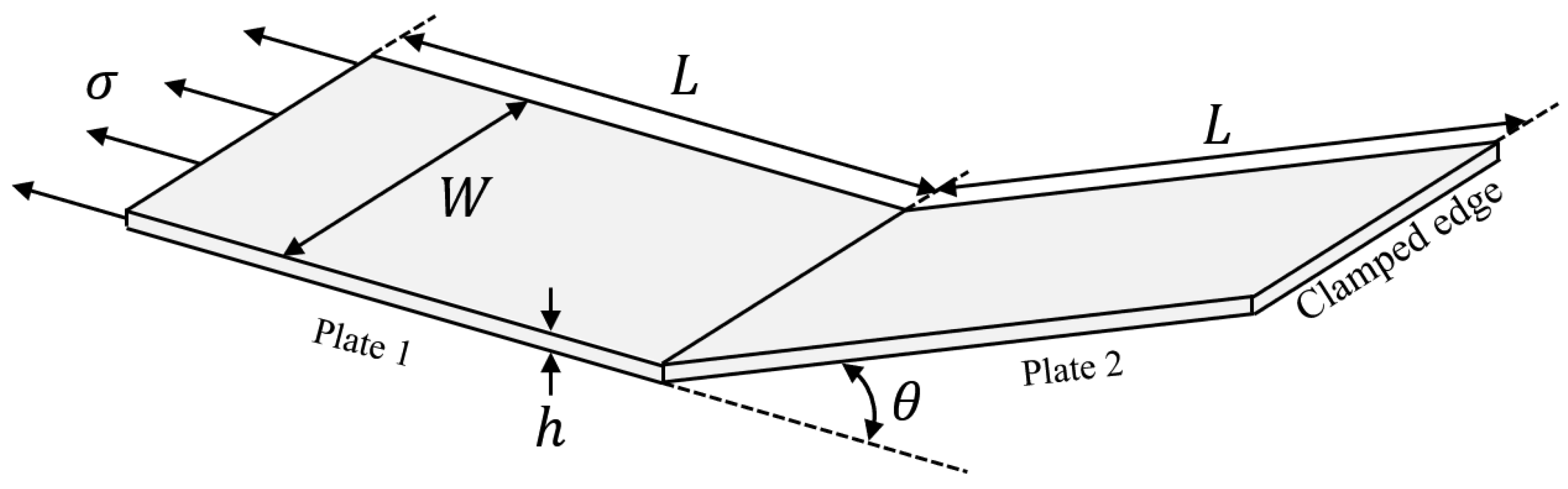
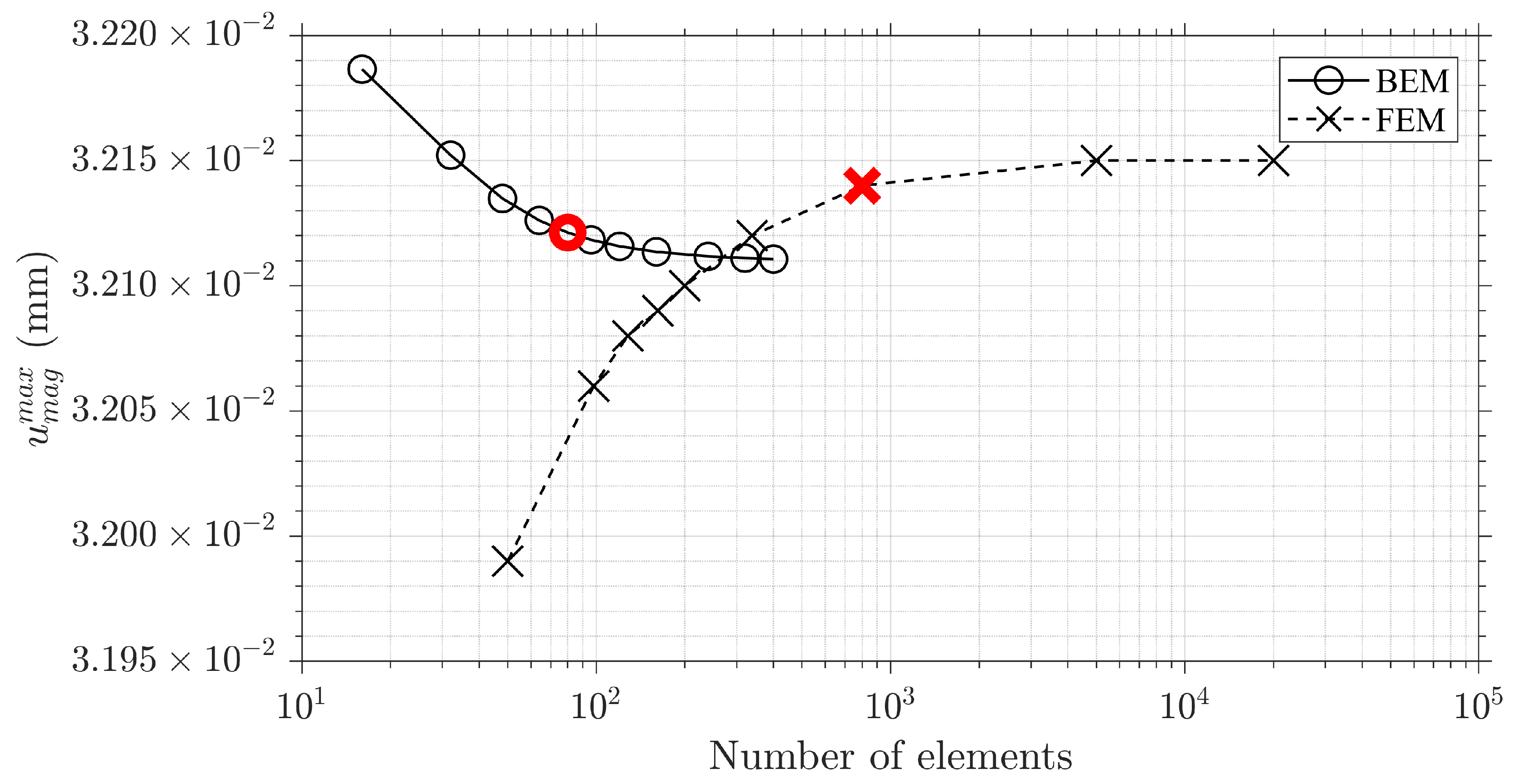
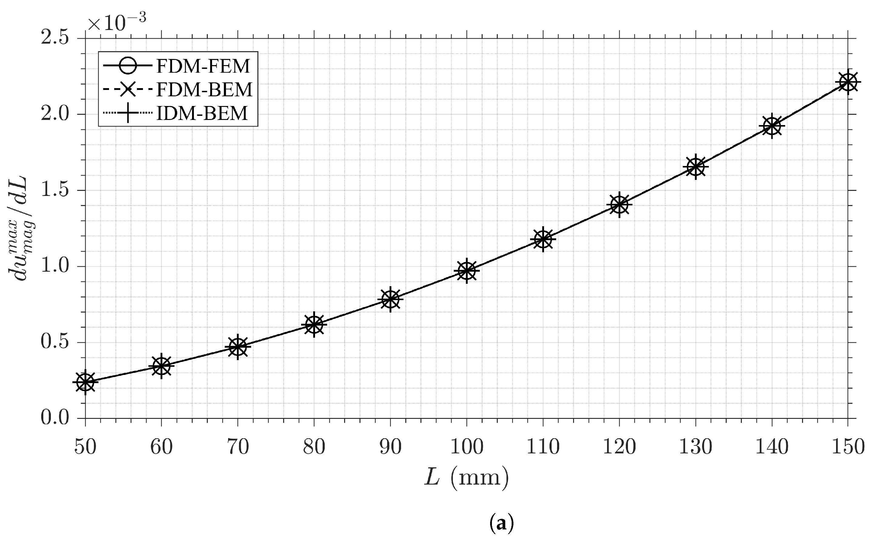
3.1. Numerical Example 1: L-Shaped Plate

To validate the developed Implicit Differentiation Method (IDM) for assembled plate structures, the L-shaped structure shown in Figure 7 was investigated. This structure is composed of two plates joined together. One plate is clamped at one of its edges, and the other plate is subjected to tension along one of its edges. The two plates are composed of steel with a Young’s modulus $E=206.8$ GPa and Poisson’s ratio $\nu =0.29$. The geometry of the structure can be defined in terms of the four parameters L, W, $\theta$, and h, as shown in Figure 7 and detailed in

Table 1. The parameters of the L-shaped plate investigated in numerical example 1.

Parameter	Description	Value
L	Length of plate 1 and 2	100 mm
W	Width of plate 1 and 2	50 mm
$\theta$	Angle of plate 2	50${}^{\circ }$
h	Thickness of plate 1 and 2	10 mm

.

The maximum displacement magnitude $u_{mag}^{max}$ occurs at the loaded edge of plate 1. To validate the IDM, the derivatives of $u_{mag}^{max}$ with respect to the parameters in Table 1 were calculated via three different methods:

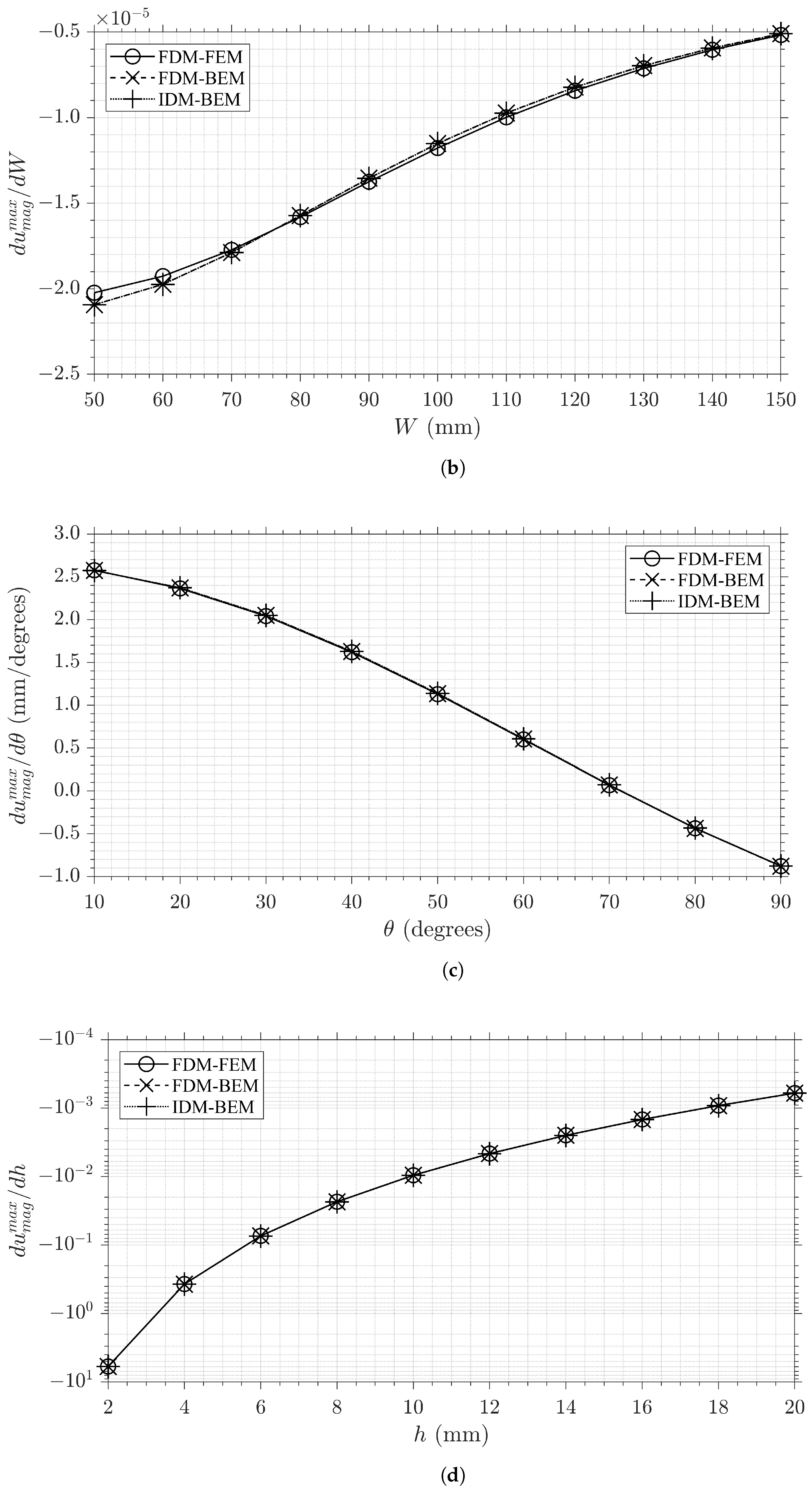
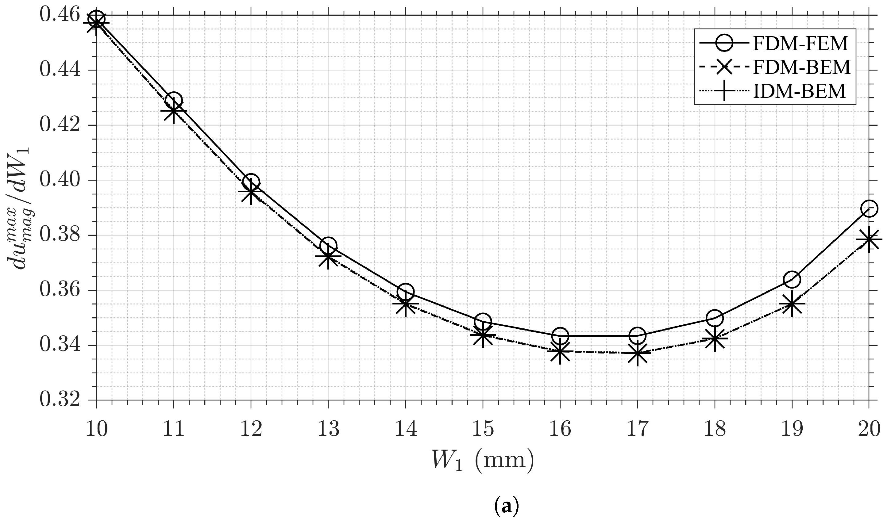
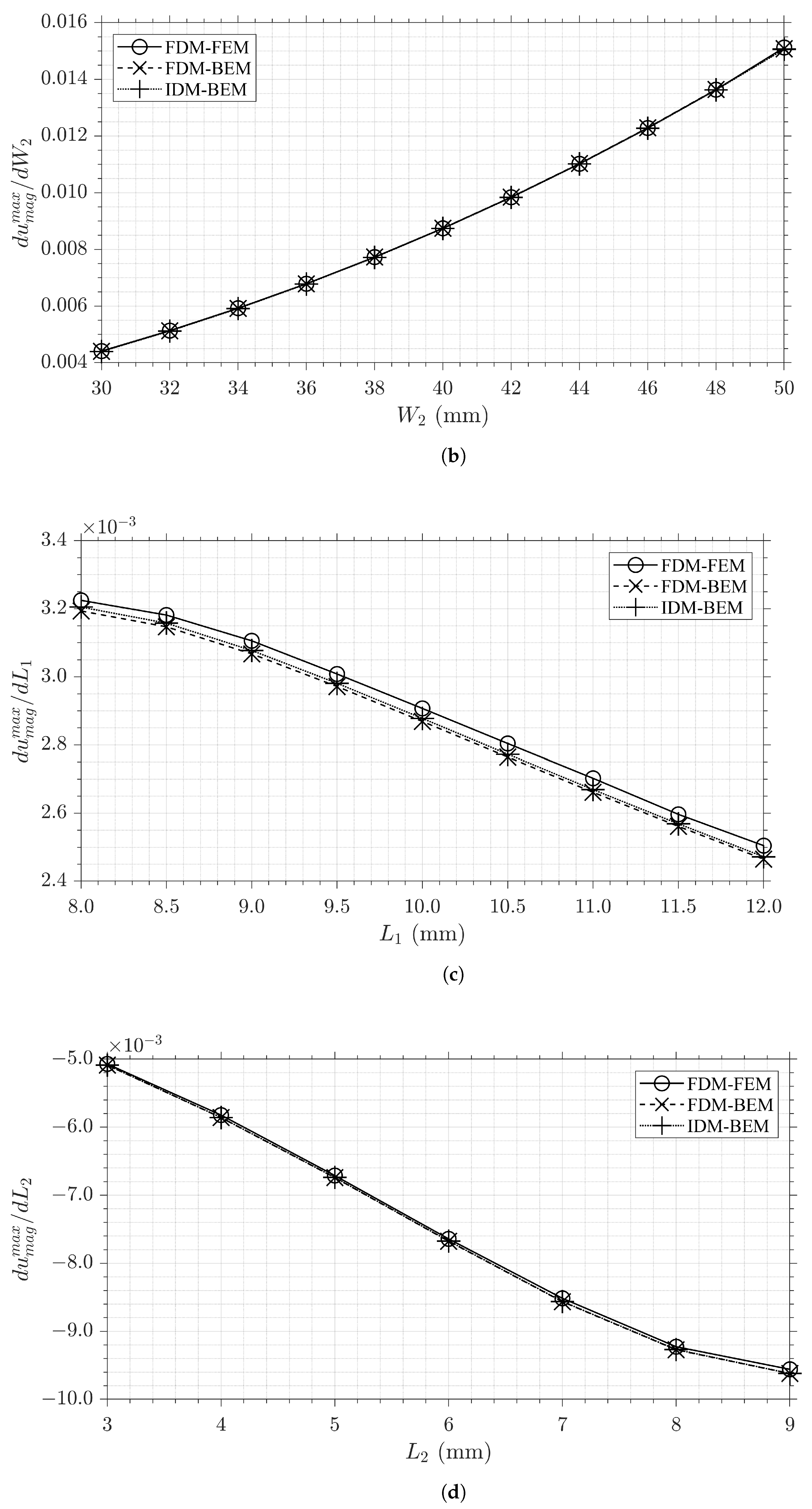
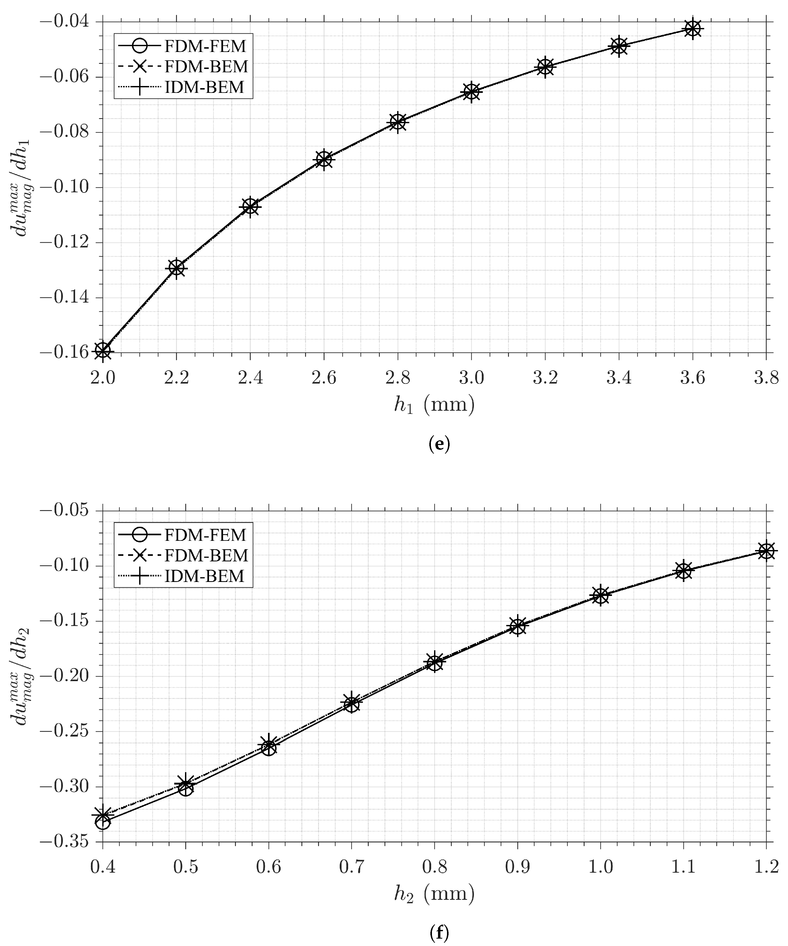
• Method 1: The IDM methodology described in Section 2. This method is referred to as ‘IDM-BEM’.
• Method 2: The BEM with the forward Finite Difference Method (FDM). This method is referred to as ‘FDM-BEM’.
• Method 3: The Finite Element Method (FEM) with the forward FDM. This method is referred to as ‘FDM-FEM’. The FEM software Abaqus FEA was used in this work.

Before a comparison can be made between these three methods, a mesh convergence study must be carried out for the BEM and the FEM. The results are shown in Figure 8. The BEM mesh is considered to have reached convergence with 80 elements, whereas the FEM mesh is considered to have reached convergence with 800 elements. These two converged meshes are shown as red markers in Figure 8.

Using the converged meshes for the BEM and the FEM, the sensitivities of $u_{mag}^{max}$ with respect to the parameters in Table 1 can be calculated using the three methods introduced earlier. The results are shown in Figure 9.

It is shown in Figure 9 that there is excellent agreement between the three methods ‘IDM-BEM’, ‘FDM-BEM’, and ‘FDM-FEM’. The average difference between IDM-BEM and FDM-FEM was, at most, only 1.9% for W, and only 0.11% for L. The average difference between IDM-BEM and FDM-BEM was even smaller, and was, at most, 0.61% for $\theta$ and only 0.073% for W. The excellent agreement between IDM-BEM and FDM-FEM, and between IDM-BEM and FDM-BEM, demonstrates the very high accuracy of the IDM when calculating sensitivities.

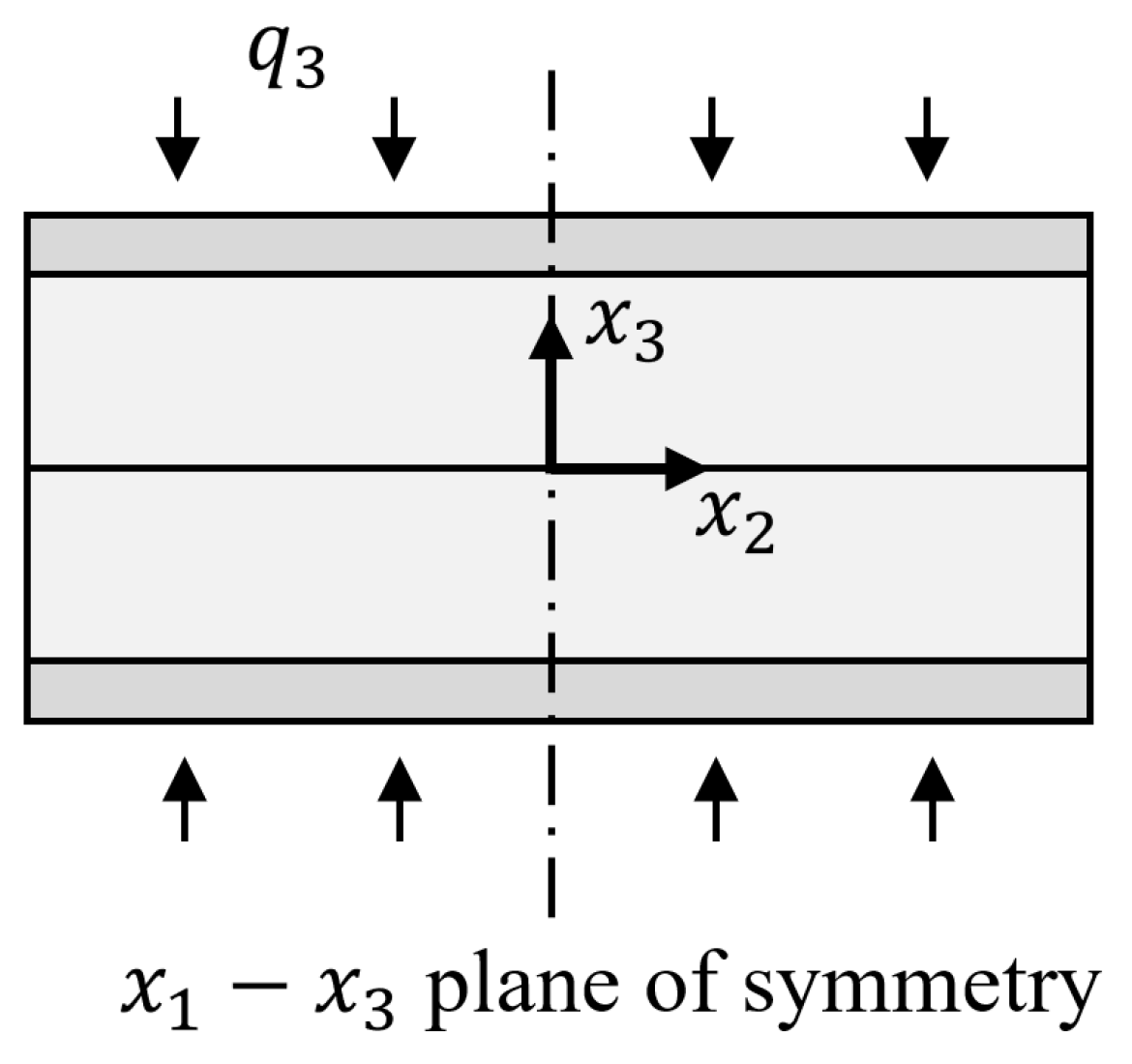
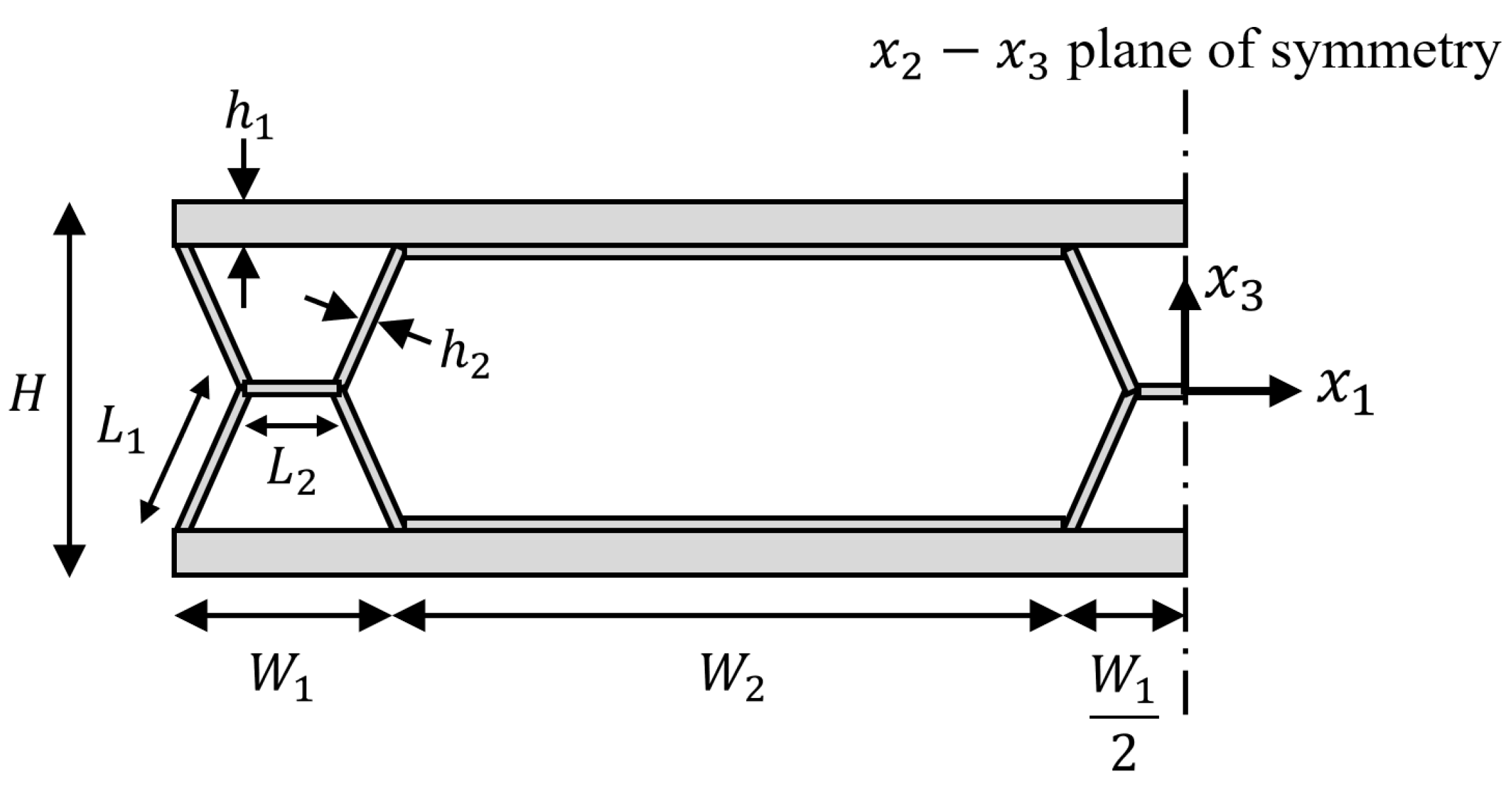
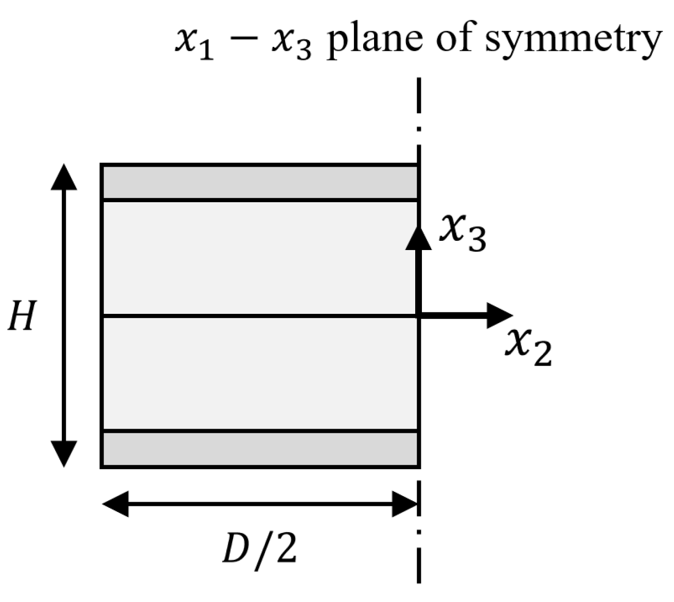
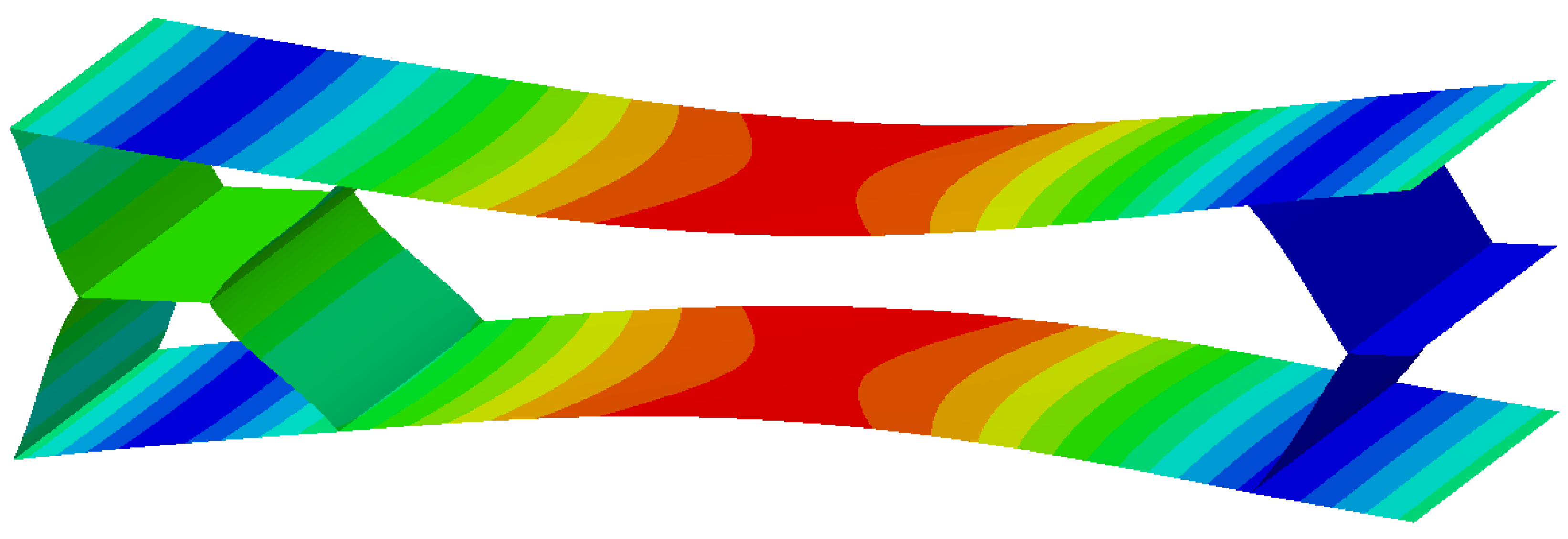
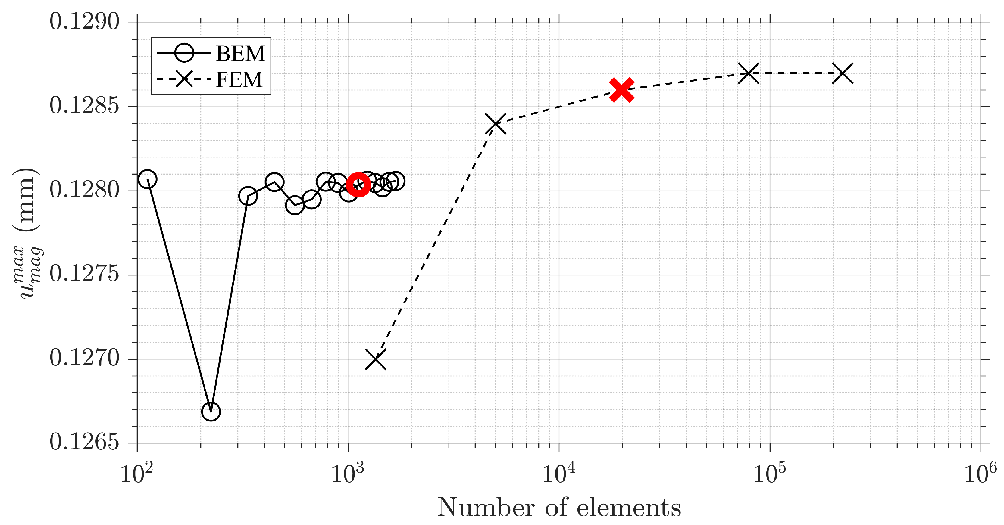
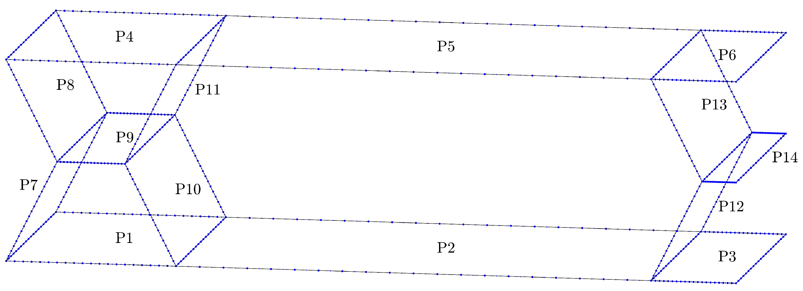
3.2. Numerical Example 2: X-Core

To further validate the developed Implicit Differentiation Method (IDM) for assembled plate structures, a significantly more complex structure was investigated with many more geometrical parameters.

The Eurofighter Typhoon has canards to increase its manoeuvrability, as shown in Figure 10. These canards are made of titanium and are manufactured using super-plastic forming and diffusion bonding, which results in a continuously connected structure. A cross-section of one of these canards is shown in Figure 11. It consists of eight X-core sections. An approximation of this cross-section is shown in Figure 12 (front-view) and in Figure 13 (side-view). The cross-section was subjected to the uniform pressure loading $q_3=1$ MPa on the top and bottom surfaces.

The canard cross-section has two planes of symmetry; these are plane $x_2-x_3$ in Figure 12 (front-view) and plane $x_1-x_3$ in Figure 13 (side-view). By using these planes of symmetry, a simplified cross-section can be obtained, as shown in Figure 14 (front-view) and Figure 15 (side-view). The geometry of this simplified cross-section can be described in terms of the six variables $W_1$, $W_2$, $L_1$, $L_2$, $h_1$, $h_2$ and also the height H and depth D, details of which are shown in

Table 2. The parameters of the X-core structure investigated in numerical example 2.

Parameter	Description	Value
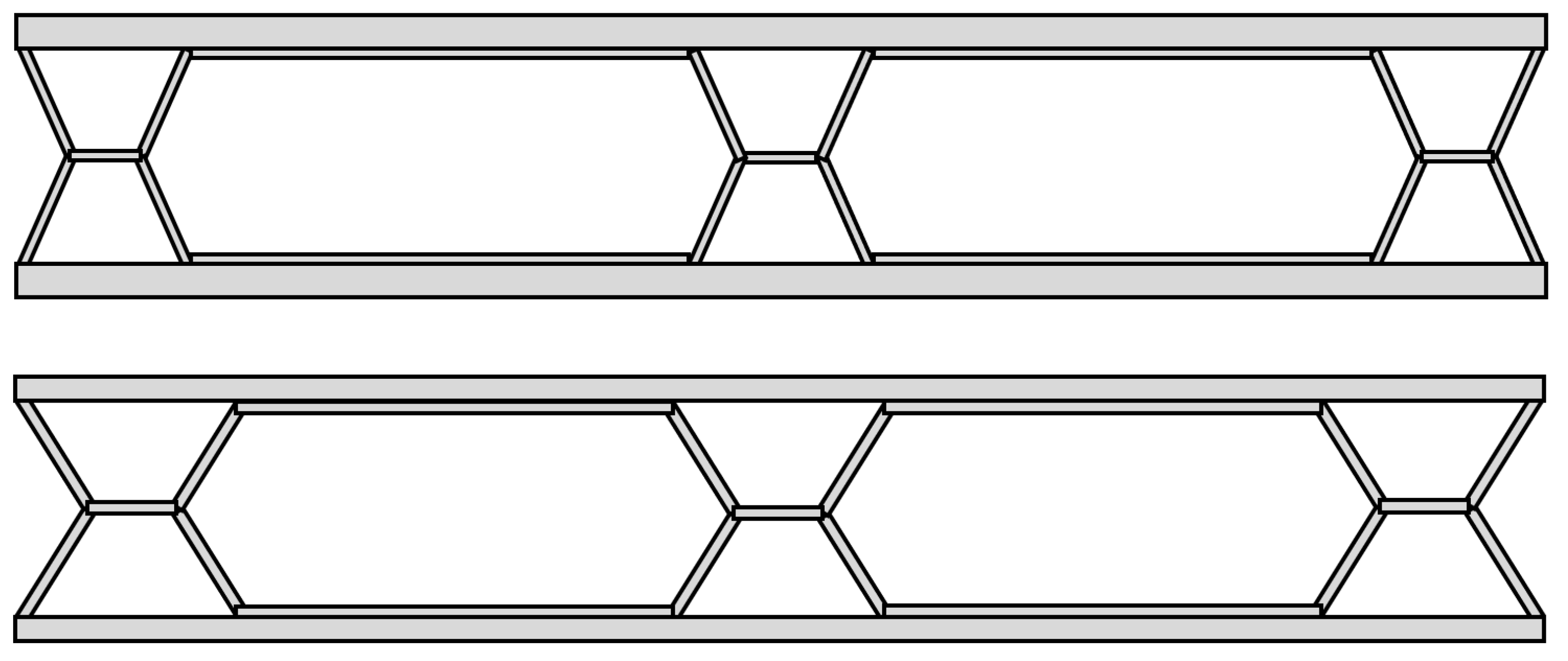
$W_1$	Width of outer long plate	15 mm
$W_2$	Width of outer short plate	42 mm
$L_1$	Length of inner inclined plate	10 mm
$L_2$	Length of inner horizontal plate	6 mm
$h_1$	Thickness of outer plate	2.8 mm
$h_2$	Thickness of inner plate	0.8 mm
H	Height	21.5 mm
D	Depth	25 mm

. The structure is made of titanium with a Young’s modulus $E=110$ GPa and Poisson’s ratio $\nu =0.3$. The structure has symmetry boundary conditions along the planes of symmetry.

The BEM model consists of 14 individual plates joined together. Symmetric boundary conditions were applied along the edges corresponding to the $x_2-x_3$ and $x_1-x_3$ planes of symmetry such that the displacement in direction $x_1$ is zero ($u_1=0$) for edges on the plane $x_2-x_3$ and the displacement in direction $x_2$ ($u_2=0$) for edges on the plane $x_1-x_3$. For the node corresponding to the centre of the coordinate system (0,0,0), the vertical displacement was set to zero ($w_3=0$).

A displacement contour plot of the X-core structure is shown in Figure 16. The maximum displacement magnitude $u_{mag}^{max}$ occurs at the middle of the top and bottom plates. To validate the IDM, the sensitivities of $u_{mag}^{max}$ with respect to the parameters in Table 1 were calculated via the three different methods introduced in Section 3.1: ‘IDM-BEM’, ‘FDM-BEM’, and ‘FDM-FEM’.

Before a comparison can be made between these three methods, a mesh convergence study must be carried out for the BEM and the FEM. The results of this mesh convergence study are shown in Figure 17. The BEM mesh is considered to have reached convergence with 1120 elements, whereas the FEM mesh is considered to have reached convergence with 19,800 elements. These two converged meshes are shown as red markers in Figure 17. The converged BEM mesh is shown in Figure 18 and it is composed of 14 individual plates joined together.

Using the converged meshes for the BEM and the FEM, the sensitivities of $u_{mag}^{max}$ with respect to the parameters in Table 2 can be calculated using the three methods introduced earlier. The results are shown in Figure 19.

It is shown in Figure 19 that there is excellent agreement between the three methods ‘IDM-BEM’, ‘FDM-BEM’, and ‘FDM-FEM’. The average difference between IDM-BEM and FDM-FEM was, at most, only 1.5% for $W_1$, and only 0.29% for $h_1$. The average difference between IDM-BEM and FDM-BEM was even smaller, and was, at most, 0.31% for $L_1$, and only 0.034% for $L_2$. The excellent agreement between IDM-BEM and FDM-FEM and between IDM-BEM and FDM-BEM demonstrates the very high accuracy of the IDM when calculating sensitivities for this very complex example.

To compare the computational efficiency of the three methods, they were each used to calculate 100 sensitivities of the X-core structure. This comparison is shown in

Table 3. CPU time to calculate 100 sensitivities using each of the three methods.

Method	CPU Time (s)
FDM-FEM	1120
FDM-BEM	1149
IDM-BEM	870

. It is shown that the methods ‘FDM-FEM’ and ‘FDM-BEM’ require a similar amount of CPU time (1120 s vs. 1149 s) to calculate 100 sensitivities. The method ‘IDM-BEM’ is significant more computationally efficient than the other two methods—it is 22% faster than ‘FDM-FEM’ and 24% faster than ’FDM-BEM’.

3.3. Numerical Example 3: Shape Optimisation of the X-Core

The previous two numerical examples validated the newly developed IDM for assembled structures with a simple example and with a significantly more complex example. To demonstrate how the IDM could be used in practice, it is used in this example to optimise the shape of the X-core structure investigated in the previous numerical example.

The shape of the X-core structure was optimised such that its mass was minimised while the maximum displacement magnitude $u_{mag}^{max}$ was less than 0.1 mm. The height H and depth D of the X-core were also fixed at 21.5 mm and 25 mm, respectively. The total width of the X-core $W_{tot}=3W_1+2W_2$ was also fixed at 129 mm. The optimisation problem is shown in Equation (52):

$$\begin{array}{cc}\hfill & \mathrm{Minimise}:Mass\left(\mathbf{d}\right)\hfill \\ \hfill & \mathrm{Subject} \mathrm{to}:{\mathbf{d}}^L\le \mathbf{d}\le {\mathbf{d}}^U,\mathbf{d}\in {\mathbb{R}}^{n_d}\hfill \\ \hfill & u_{mag}^{max}\le 0.1\mathrm{mm}\hfill \\ \hfill & H=21.5\mathrm{mm}\hfill \\ \hfill & D=25\mathrm{mm}\hfill \\ \hfill & W_{tot}=3W_1+2W_2=129\mathrm{mm}\hfill \end{array}$$

(52)

where the design variables are $\mathbf{d}=[W_1,W_2,L_1,L_2,h_1,h_2]$, and $n_d=6$. The initial design is ${\mathbf{d}}_0=[15,42,10,6,2.8,0.8]$. The lower and upper bounds are: ${\mathbf{d}}^L=0.75\times {\mathbf{d}}_0$ and ${\mathbf{d}}^U=1.25\times {\mathbf{d}}_0$. The mass can be calculated using the design variables $\mathbf{d}$ and the density of titanium $\rho =4.41\times {10}^{-3}$ g/mm³.

The IDM was used to solve the above optimisation problem. The optimisation procedure was stopped once the relative change in mass between iterations fell to below 0.1% and $u_{mag}^{max}$ below or equal to 0.1 mm with a tolerance of 0.001 mm. The results of this optimisation procedure can be seen in Figure 20. It is shown in this Figure that the optimisation procedure successfully minimised the mass of the X-core structure—the mass was initially 27 g and was reduced to 23.5 g after 62 iterations. The maximum displacement magnitude $u_{mag}^{max}$ was initially 0.139 mm and was reduced to 0.101 mm after 62 iterations.

The shape and the values for the shape parameters of the X-core structure before and after the shape optimisation procedure are shown in Figure 21 and

Table 4. The parameters of the X-core structure before and after shape optimisation.

Shape Parameter (mm)
Design	${\mathit{W}}_{\mathbf{1}}$	${\mathit{W}}_{\mathbf{2}}$	${\mathit{L}}_{\mathbf{1}}$	${\mathit{L}}_{\mathbf{2}}$	${\mathit{h}}_{\mathbf{1}}$	${\mathit{h}}_{\mathbf{2}}$	$\mathit{H}$	$\mathit{D}$	${\mathit{W}}_{\mathit{tot}}$	Mass (g)	${\mathit{u}}_{\mathit{mag}}^{\mathit{max}}$(mm)
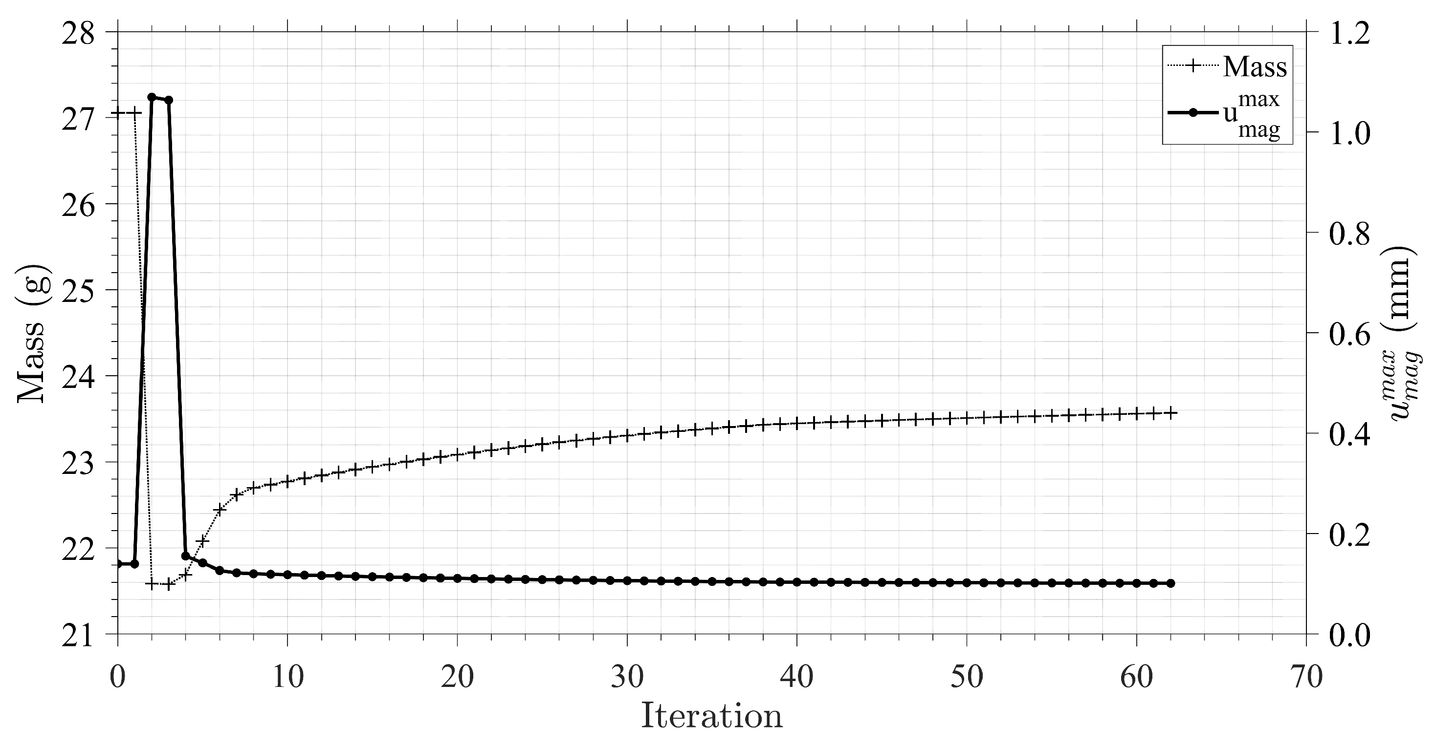
Before	15.0	42.0	10.0	6.0	2.8	0.80	21.5	25	129	27.0	0.139
After	18.8	36.4	10.8	7.5	2.1	0.98	21.5	25	129	23.5	0.101

. It is shown that the height H and depth D of the X-core structure are unchanged, which was expected. The width of the X-sections have been made wider and the thickness of the inner plates has also been increased, whereas the thickness of the outer plates has been reduced. This had the effect of reducing the mass of the X-core structure and its maximum displacement magnitude $u_{mag}^{max}$.

In summary, this numerical example demonstrated the effectiveness of the IDM when used in practice for optimising the shape of a complex assembled structure, such as an X-core structure with many geometric design variables.

4. Conclusions

In conclusion, a novel methodology was presented for conducting sensitivity analyses of assembled plate structures using the Boundary Element Method (BEM). The main novelty of this work was that the exact implicit derivatives of the BEM formulations for assembled plate structures were derived for the first time and incorporated into a newly developed Implicit Differentiation Method (IDM) for performing structural sensitivity analyses—enabling sensitivity analyses to be conducted for more complex and realistic structures in a more accurate, robust, and efficient manner. Several numerical examples were presented to validate the derived exact implicit derivatives and to demonstrate how they could be used for a potential application involving the shape optimisation of a complex X-core structure from the canard of a Eurofighter Typhoon fighter jet. The values of six geometrical parameters were optimised to minimise the maximum displacement in the X-core. The newly developed IDM was found to be very similar in terms of accuracy to the Finite Difference Method (FDM), demonstrating percentage differences less than 2%. The IDM was also found to be over 20% more computationally efficient than the FDM. Furthermore, unlike the FDM, the IDM does not require a step-size, meaning that, compared to the FDM, the IDM is significantly more robust. Potential applications include the shape optimisation or structural reliability analysis of complex plate structures.

Future work will aim to develop an IDM for assembled shell structures, enabling the sensitivity analysis of complex aircraft structures such as fuselage panels or wing sections. Sensitivity analyses involving buckling and large-deflections will also be investigated to expand the range of possible applications.

References

- Aliabadi, M.H. The Boundary Element Method: Applications in Solids and Structures; John Wiley and Sons: Chichester, UK, 2002; Volume 2. [Google Scholar]
- Tafreshi, A. Shape optimization of two-dimensional anisotropic structures using the boundary element method. J. Strain Anal. Eng. Des. 2003, 38, 219–232. [Google Scholar] [CrossRef] [Green Version]
- Abe, K.; Kazama, S.; Koro, K. A boundary element approach for topology optimization problem using the level set method. Commun. Numer. Methods Eng. 2006, 23, 405–416. [Google Scholar] [CrossRef]
- Canelas, A.; Herskovits, J.; Telles, J.C.F. Shape optimization using the boundary element method and a SAND interior point algorithm for constrained optimization. Comput. Struct. 2008, 86, 1517–1526. [Google Scholar] [CrossRef]
- Ullah, B.; Trevelyan, J. Correlation between hole insertion criteria in a boundary element and level set based topology optimisation method. Eng. Anal. Bound. Elem. 2013, 37, 1457–1470. [Google Scholar] [CrossRef] [Green Version]
- Chang, Y.; Cheng, H.; Chiu, M.; Chien, Y. Shape Optimisation of Multi-Chamber Acoustical Plenums Using BEM, Neural Networks, and GA Method. Arch. Acoust. 2016, 41, 43–53. [Google Scholar] [CrossRef] [Green Version]
- Ullah, B.; Trevelyan, J. A boundary element and level set based topology optimisation using sensitivity analysis. Eng. Anal. Bound. Elem. 2016, 70, 80–98. [Google Scholar] [CrossRef] [Green Version]
- Liu, C.; Chen, L.; Zhao, W.; Chen, H. Shape optimization of sound barrier using an isogeometric fast multipole boundary element method in two dimensions. Eng. Anal. Bound. Elem. 2017, 85, 142–157. [Google Scholar] [CrossRef]
- Ullah, B.; Trevelyan, J.; Sirajul, I. A boundary element and level set based bi-directional evolutionary structural optimisation with a volume constraint. Eng. Anal. Bound. Elem. 2017, 80, 152–161. [Google Scholar] [CrossRef] [Green Version]
- Takahashi, T.; Yamamoto, T.; Shimba, Y.; Isakari, H.; Matsumoto, T. A framework of shape optimisation based on the isogeometric boundary element method toward designing thin-silicon photovoltaic devices. Eng. Comput. 2018, 35, 423–449. [Google Scholar] [CrossRef]
- Matsushima, K.; Isakari, H.; Takahashi, T.; Matsumoto, T. A topology optimisation of composite elastic metamaterial slabs based on the manipulation of far-field behaviours. Struct. Multidiscip. Optim. 2020, 63, 231–243. [Google Scholar] [CrossRef]
- Maduramuthu, P.; Fenner, R.T. Three-dimensional shape design optimization of holes and cavities using the boundary element method. J. Strain Anal. Eng. Des. 2004, 39, 87–98. [Google Scholar] [CrossRef]
- Bandara, K.; Cirak, F.; Of, G.; Steinbach, O.; Zapletal, J. Boundary element based multiresolution shape optimisation in electrostatics. J. Comput. Phys. 2015, 297, 584–598. [Google Scholar] [CrossRef] [Green Version]
- Ullah, B.; Trevelyan, J.; Ivrissimtzis, I. A three-dimensional implementation of the boundary element and level set based structural optimisation. Eng. Anal. Bound. Elem. 2015, 58, 176–194. [Google Scholar] [CrossRef] [Green Version]
- Chen, L.L.; Lian, H.; Liu, Z.; Chen, H.B.; Atroshchenko, E.; Bordas, S.P.A. Structural shape optimization of three dimensional acoustic problems with isogeometric boundary element methods. Comput. Methods Appl. Mech. Eng. 2019, 355, 926–951. [Google Scholar] [CrossRef]
- Gaggero, S.; Vernengo, G.; Villa, D.; Bonfiglio, L. A reduced order approach for optimal design of efficient marine propellers. Ships Offshore Struct. 2019, 15, 200–214. [Google Scholar] [CrossRef]
- Li, S.; Trevelyan, J.; Wu, Z.; Lian, H.; Wang, D.; Zhang, W. An adaptive SVD–Krylov reduced order model for surrogate based structural shape optimization through isogeometric boundary element method. Comput. Methods Appl. Mech. Eng. 2019, 349, 312–338. [Google Scholar] [CrossRef] [Green Version]
- Morse, L.; Sharif Khodaei, Z.; Aliabadi, M.H. A multi-fidelity boundary element method for structural reliability analysis with higher-order sensitivities. Eng. Anal. Bound. Elem. 2019, 104, 183–196. [Google Scholar] [CrossRef]
- Morse, L.; Mallardo, V.; Aliabadi, F.M.H. Manufacturing cost and reliability-based shape optimization of plate structures. Int. J. Numer. Methods Eng. 2022, 123, 2189–2213. [Google Scholar] [CrossRef]
- Mallardo, V.; Aliabadi, M.H. A BEM sensitivity and shape identification analysis for acoustic scattering in fluid–solid problems. Int. J. Numer. Methods Eng. 1998, 41, 1527–1541. [Google Scholar] [CrossRef]
- Mallardo, V.; Alessandri, C. Inverse problems in the presence of inclusions and unilateral constraints a boundary element approach. Comput. Mech. 2000, 26, 571–581. [Google Scholar] [CrossRef]
- Morse, L.; Sharif Khodaei, Z.; Aliabadi, M.H. A dual boundary element based implicit differentiation method for determining stress intensity factor sensitivities for plate bending problems. Eng. Anal. Bound. Elem. 2019, 106, 412–426. [Google Scholar] [CrossRef]
- Brancati, A.; Aliabadi, M.H.; Mallardo, V. A BEM sensitivity formulation for three-dimensional active noise control. Int. J. Numer. Methods Eng. 2012, 90, 1183–1206. [Google Scholar] [CrossRef]
- Dirgantara, T.; Aliabadi, M.H. Crack Growth analysis of plates Loaded by bending and tension using dual boundary element method. Int. J. Fract. 1999, 105, 27–47. [Google Scholar]