1. Introduction
Micro/nano-satellites generally refer to satellites with a magnitude of 1–100 kg. Compared with conventional large satellites, micro/nano-satellites have a short development cycle, low cost, high flexibility, and low risk, and can better serve in many fields, such as meteorology, telemetry, and communication [
1]. The large-scale production and application of low-orbit satellites has become a major trend in modern satellite development because of their low cost and weight. Therefore, in the pursuit of miniaturisation of micro/nano-satellite supporting products, there are also corresponding requirements for flywheels. In a three-axis stable satellite attitude control system, the flywheel is the main actuator, its rotation speed is regulated by a high-speed motor, and the star attitude control is realised through momentum exchange with the stars [
2]. As a key mechanism for the attitude control of micro/nano-satellites, the product quality of the flywheel is directly related to the ground orientation and attitude control of the satellite, and directly affects the satellite’s life and in-orbit mission [
3]. Therefore, a micro/nano-satellite flywheel should be built on the basis of accurate optimisation to more effectively ensure the smooth operation of the satellite platform, release the payload allowance, and maximise the performance potential of the satellite platform.
In terms of satellite structure optimisation, Han Chong [
4] completed maximum first natural frequency and the smallest-quality multi-objective by combining a BP (backpropagation) neural network and genetic algorithm optimisation calculation, aiming at the requirements of small total mass and high first natural frequency of the satellite structure, and obtained reasonable design variable values. The feasibility of a BP network combined with a genetic algorithm in satellite structure optimisation was verified. Chen Shen-Yan [
5] established a finite element model of the initial scheme of a new satellite structure in the initial prototype stage. Taking the cross-section size of each beam in the main load truss as the design variable, and considering the whole-star modal frequency, strength, and stability constraints, a structural optimisation model was established to minimise the structural weight. Gu Yuanxian [
6] considered the constraints of the natural frequency and flexion stability in the optimisation design, used a variety of design variables, adopted discrete material variable continuous processing for honeycomb sandwich materials, and used the JIFEX software to optimise the design of a main load-bearing structure for large communication satellites. From the above research, we can see that there are two main ways to optimise the satellite structure: One is to choose lightweight structural materials and improve their optimisation. The other is the optimised design of the structural parameters. For the latter, the main goal of optimisation is to achieve the minimum weight under the premise of ensuring the first-order frequency of the structure—usually in the form of an intelligent optimisation algorithm and finite element parametric simulation.
Compared with satellite structural optimisation, the constraints of satellite flywheel optimisation are largely consistent with the optimisation goal, guaranteeing the maximum first-order vibration frequency and the minimum weight. However, in the finite element simulation, the load conditions—such as rotational speed and angular acceleration—should be considered. In terms of the optimisation design, there are few studies related to the flywheel. Researchers such as Ma Huaiteng [
7] optimised the design of the inertia disc of marine high-power diesel generator sets, and checked the strength of the inertia disc using Ansys Workbench. As a result, the safety factor was greatly improved compared with the initial inertia disc. However, the optimisation method was based on an empirical formula, and the results were not optimised. Xu Shihui [
8] conducted a finite element simulation analysis of centrifugal impellers using Abaqus, obtained the force characteristics of the impeller under the combination of acceleration and constant velocity, and analysed and summarised the method of impeller material selection and weight reduction.
Eigenvalues and structural vibration modes describe the vibration characteristics and frequency characteristics of the structure under free vibration. When solving the eigenvalue, one method is solving all of the eigenvalue problems of the structural system’s characteristic equation; the other is solving the partial eigenvalue problem. In structural mechanics, the matrix order is very high, and it is not necessary to solve the full eigenvalues and eigenvectors. In the solution method, there are two categories: the direct method and the vector iteration method. Both the Lanczos technique and the subspace iteration in the FEM analysis software Abaqus are considered to be vector iteration methods [
9]. Using the MSC/NASTRAN finite element software, Shan Tilei designed the overall configuration of the satellite, which showed that the optimised satellite structure has a high-strength and high-stiffness structure-carrying capacity and good-quality characteristics [
10].
For the objective function, the optimisation methods can be divided into single-objective optimisation and multi-objective optimisation. For the former, the optimisation procedure is driven by a single objective function to find the optimal solution to the optimisation parameters. In the second case, the processes driven by multiple objective functions eventually achieve the trade-off between them.
Optimisation algorithms can be used to find optimal solutions for a particular problem, or a set of optimal solutions in a specific design space, for which they have been widely used in many fields. A large number of optimisation algorithms have been developed based on different numerical methods or logic strategies for specific problems. These methods can generally be divided into numerical optimisation algorithms and global optimisation algorithms. Numerical optimisation algorithms, such as the feasible direction algorithm [
11] and the nonlinear conjugate gradient algorithm [
12], are generally much faster than global optimisation algorithms. However, the results of the numerical optimisation algorithms are highly dependent on the initial values, which may lead to local optimisation if the initial search point is not appropriate. Global optimisation algorithms can achieve global optimisation without calculating the local gradient, with no strict requirements for the initial search point. Typical global optimisation algorithms include the simulated annealing algorithm [
13], the genetic algorithm [
14,
15], and the particle swarm optimisation algorithm [
16].
The non-dominant classification genetic algorithm (NSGA-II) was proposed by Deb et al. [
17,
18,
19]. On the basis of the non-dominant ranking genetic algorithm based on the Pareto optimisation concept (NSGA [
20]), the defect of high NSGA operation complexity is overcome, and the algorithm’s performance is greatly improved. NSGA-II considers both crowd computing and elite strategies, using the crowd comparison operator that reduces the computational complexity of the algorithm and avoids local convergence in the optimisation process. Based on the notion of the Pareto-optimal solution, the weights of each objective function do not require an artificial distribution, and result in a non-inferior set of solutions. Individuals at the Pareto-optimal boundary can be uniformly extended to the entire solution space, ensuring the population diversity with high efficiency and robustness.
In some structural design and development stages, the performance of the engineering structure is optimised by the finite element simulation technology, shortening the cycle of analysis and design to a certain extent. However, with increasing computer speed, the accuracy requirements of the FEM simulation analysis are also improved accordingly—especially for a large number of complex and fine engineering structures—and the computational cost of completing an engineering FEM simulation analysis with high fidelity is greatly increased. At the same time, with the proposal and research of multidisciplinary optimisation design, the optimisation design of engineering structures often needs a lot of simulation analysis to obtain the system response values of different design variable combinations, so it can be seen that relying only on finite element simulation technology is not in line with the engineering reality. Therefore, the development of computer capabilities does not significantly shorten the optimisation design cycle of actual complex engineering structures, but increases the complexity of finite element modelling. In order to scientifically reduce the number of complex and time-consuming simulation calculations to a certain extent, the agent model technology was developed and improved, and has been gradually applied to actual complex engineering optimisation in various fields as a research hotspot [
21].
The agent model, also known as the approximate model, is a mathematical model mainly based on a small number of finite element sample points and the corresponding response values based on finite element simulation or physical tests. The constructed model has a low calculation complexity and fast calculation speed, but the calculation results are close to the actual results. Therefore, the model can be used to replace the actual optimisation problem, and then reduce the number of time-consuming finite element calculations in order to meet the requirements of effectively shortening the design cycle and computer cost in the optimisation design of complex engineering structures. The current commonly used approximate models include, among others, the polynomial response surface models, the Kriging model [
22,
23], the radial basis function (RBF) model [
24,
25], the support-vector machine model, and the neural network model. The radial basis model has a simple form, homogeneity, few setting parameters, and easy processing, and is widely used for both high-dimensional and nonlinear problems.
2. Theory
2.1. Flying Wheel Design Theory
Satellite attitude control includes two main control methods: jet control, and angular momentum exchange control. High-precision, long-life, three-axis stable satellites generally use a wheel control scheme; that is, using the angular momentum exchange device as the control system actuator.
The wheel control system is based on the momentum moment theorem—the size and direction of the flywheel produce the reaction moment acting on the satellite, which then changes the momentum moment of the main body of the satellite.
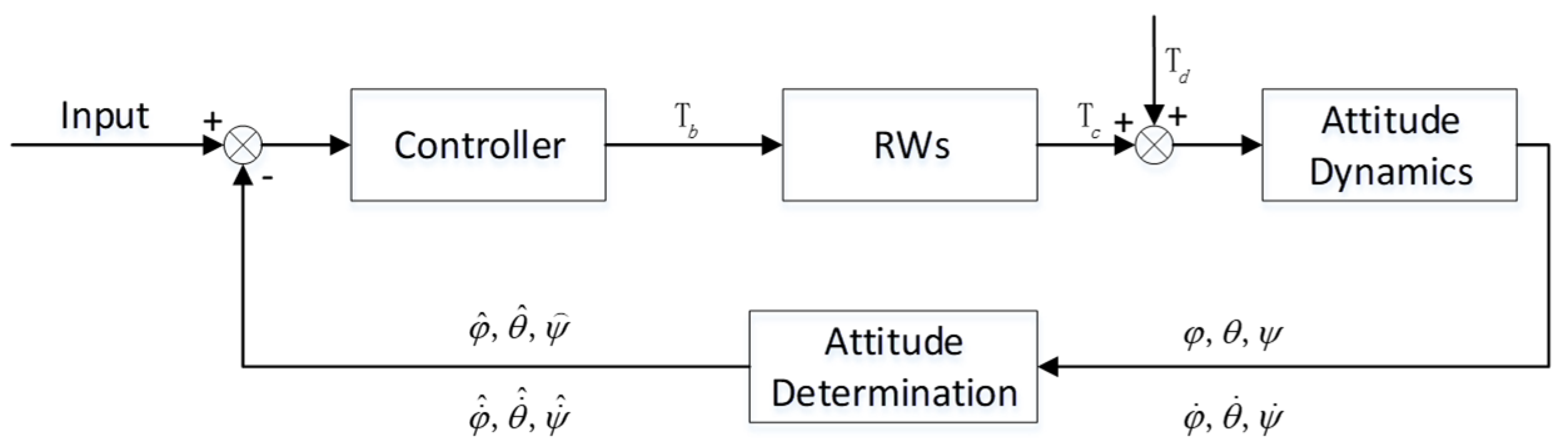
The wheel control system is divided into a zero-momentum control system and a bias control system. The zero-momentum control system is applied to satellites with high stability requirements. Taking the zero-momentum control system as an example, we have the following [
26]. Block diagram of the satellite zero-momentum system is as shown in
Figure 1.
Where 𝑇𝑏 is the theoretical control torque; 𝑇𝑑 is the actual control torque; 𝑇c is the component array of external moments in the stellar coordinate system; 𝜑, 𝜃, and 𝜓 are the three-axis attitude angles; , , and are the three-axis attitude angular velocities; , , and are the three-axis estimated attitude angles , , and are the three-axis attitude estimated angular velocities; and RWs is the flywheels combination.
Satellite pose dynamics model of the three-orthogonal flywheel [
26]:
where 𝐼
𝑏 is the component array of inertia and vector in the stellar coordinate system, 𝑤𝑏 is the component matrix of the angular velocity vector in the stellar coordinate system, 𝐽
𝑤 is the diagonal array of rotational inertia of three flywheels, Ω
𝑤 is the array of the rotational speed of three flywheels, and 𝑇
𝑑 is the component array of external moments in the stellar coordinate system.
Simplified to the near-circular orbit, the satellite coordinate system coincides with the main inertia axis. The component array and attitude angular velocity relationship of the satellite’s angular velocity vector in the satellite coordinate system is
:
where 𝜑, 𝜃, and 𝜓 are the three-axis attitude angles;
,
, and
are the three-axis attitude angular velocities; and 𝑤𝑜 is the angular velocity of the Earth’s rotation.
For high-orbit or inertial directional satellites, we can bring in the kinetic model and omit the minor terms:
In summary, for high-orbiting or inertially oriented satellites, the three channels of the attitude dynamics control model are decoupled, and each channel’s mathematical model can be considered as a double-integral link.
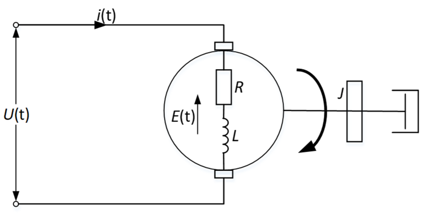
The real flywheel mathematical model based on rotational speed control is nonlinear. After linearisation, the simplified model is as follows [
26,
27]:
where ℎ(𝑠)𝑠 is the actual control torque, 𝑇
𝑐(𝑠) is the desired control torque, 𝐾
𝑚 is the torque constant, 𝑅 is the armature resistance, 𝐾
𝑒 is the potential constant, 𝐽 is the rotor and flywheel rotational inertia of the motor, and
is a constant scale factor. Model diagram of the flywheel motor shows in
Figure 2.
The relationship between command torque and rotor speed satisfies the following equation:
where
is the inertia disc speed,
t is the time, and 𝑇
w is the torque.
In conclusion, the size of inertia of the satellite largely determines the efficiency of the flywheel. In addition, the requirements of light weight and miniaturisation should be met. Based on this, the following flywheel evaluation factor is proposed:
where
c is a constant term,
M is the mass of the inertia disc, and
Fre1 is the first-order vibration frequency of the flywheel. In the flywheel optimisation process, the larger the value of
Re, the more suitable the obtained flywheel is for the nano-satellite platform.
2.2. The RBF Radial Basis Response Model
The RBF model uses the Hardy method introduced in the literature by Kansa [
25,
27], assuming the set of points
x1, …,
xN ∈ Ω ⊂ ℜ
N, such that the set of any radial basis functions
gi(
x) =
g(‖
x −
xj‖) ∈ ℜ,
j = 1, 2,…,
N, where ‖
x −
xj‖ is the Euclidean distance, which is calculated as
(𝑥 − 𝑥
𝑗). Given the data points
x1, …,
xN ∈ Ω ⊂ ℜ
N, the corresponding interpolation is
y1, …,
yN ∈ Ω ⊂ ℜ
N.
By solving the
N + 1 linear system of equations in
N + 1, the unknown expansion coefficients 𝛼
j are as follows:
Obtain the RBF interpolation:
Introduce:
where
and
; the following matrix relationship can be obtained:
The interpolation coefficient can be obtained after finding the inverse:
This gives the derivative at the interpolation point , 𝑖 = 1, 2,…, 𝑁.
The basis function used in this work is a function with a variable power spline that can adjust and approximate a large number of other functions:
The parameter c in Equation (15) is the shape function variable, with a value of 0.2~3.
For the fitted model, R-squared was generally used to assess the degree of data fitting:
where
N is the number of samples,
Yi(
i = 1 …
N) represents the original data,
is the mean of the original data, and
F(
xi)(
i = 1 …
N) is the interpolated value.
2.3. Model Optimisation
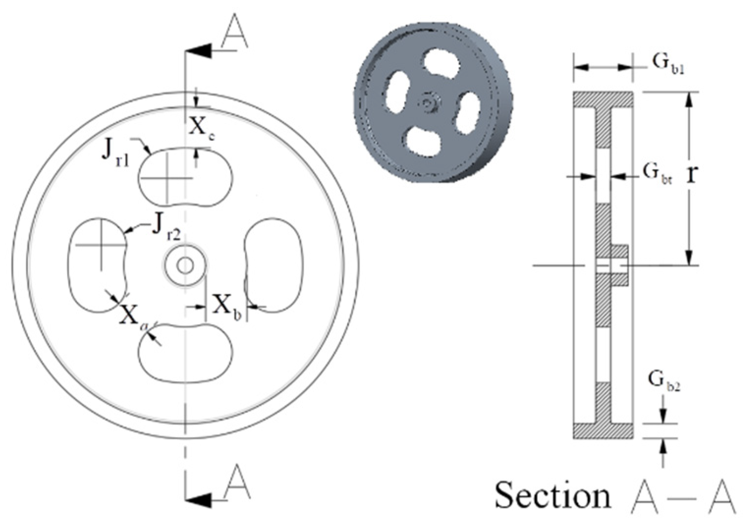
The flywheel profile parameters are shown in
Figure 3, with a total of nine optimised parameters: 𝑋
𝑎, 𝑋
𝑏, 𝑋
𝑐, 𝐽
𝑟1, 𝐽
𝑟2, 𝐺
𝑏1, 𝐺
𝑏2, and 𝐺
𝑏𝑡.
Where 𝑋
𝑎, 𝑋
𝑏, 𝑋
𝑐, 𝐽
𝑟1, 𝐽
𝑟2, 𝐺
𝑏1, 𝐺
𝑏2, and 𝐺
𝑏𝑡 are the size parameters of the flywheel. For the flywheel optimisation target, in addition to the flywheel evaluation factor Re mentioned above, the first-order vibration frequency characterising the inertia disc stiffness is also one of the targets. In order to improve the optimisation quality of the optimisation model, it is necessary to narrow the optimisation parameter interval and prevent the algorithm from falling into the local optimum to affect the final result. This work divides the optimisation model into the initial optimisation model and the final optimisation model. The initial optimisation model for the flywheel is as follows:
where
M is the flywheel mass, 𝐹𝑟𝑒1 is the flywheel’s first-order frequency, and
is the set upper mass limit. Max_mises is the maximum Mises stress, and 𝛿
𝑠 is the material yield strength. The ‘0’ in the subscript _0
dn represents the initial set value, and
_dn represents the lower limit of the interval. The ‘0’ in the subscript _0
up represents the initial set value, and
_up represents the upper limit of the interval. The difference between the final optimisation model and the initial optimisation model is the interval of the optimisation variables, as follows:
where the lower corner standard
_dn represents the lower limit of the optimisation parameter interval, and the lower corner standard
_up represents the upper limit of the optimisation parameter interval.
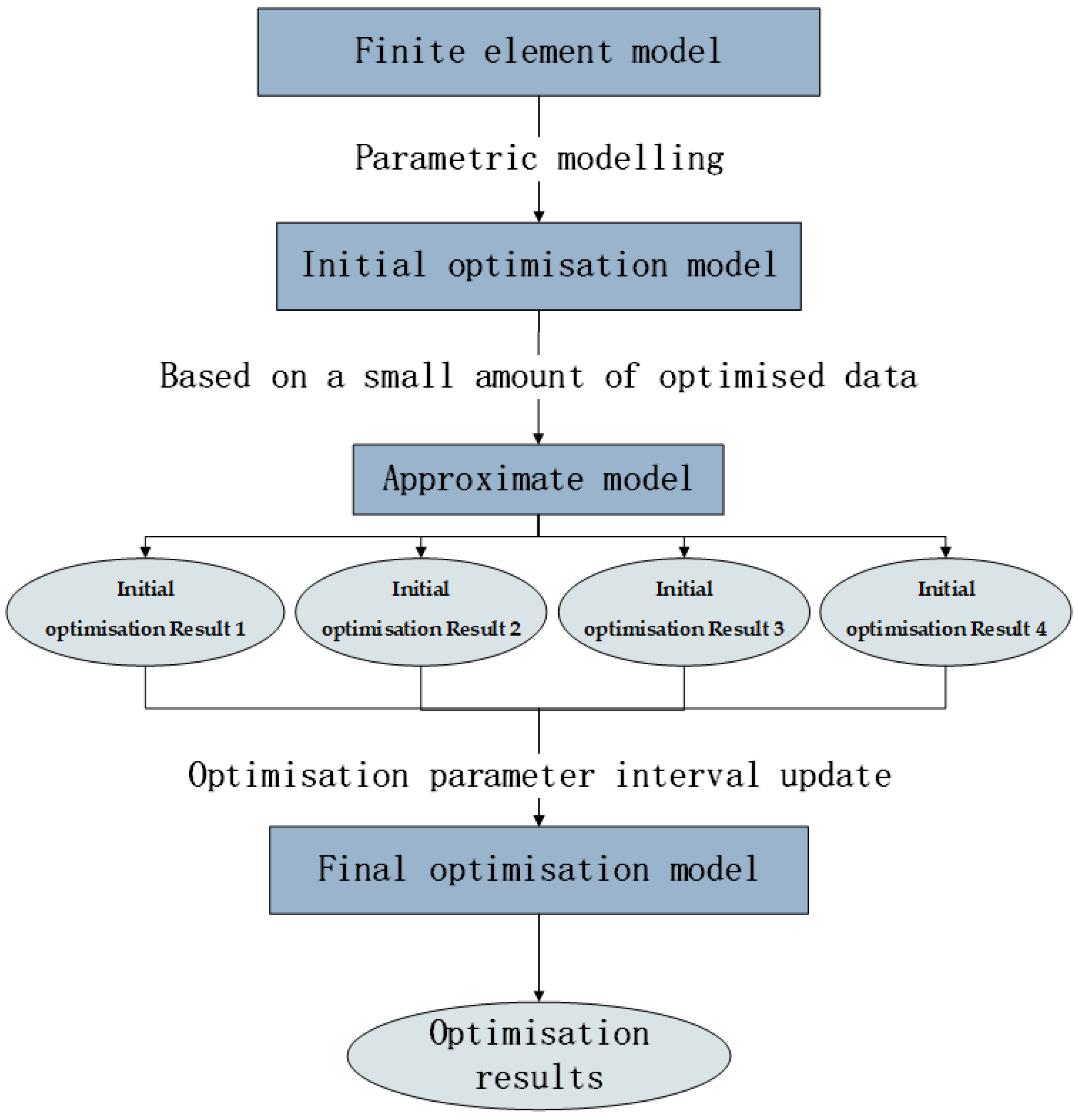
The specific optimisation steps of this paper are shown in
Figure 4, where Initial Optimisation Results 1–4 refer to four sets of optimisation parameter results obtained by four calculations using the initial optimisation model. The optimisation times can also be changed according to the corresponding situation.
The range of optimisation parameters of the optimisation model is generally determined according to practical engineering design experience. In certain situations, such as designing a particular product, the range of optimisation values may vary with the design goal, but this is also based on engineering experience. In order to avoid such a large optimisation parameter range resulting in low optimisation efficiency or the model falling into the local optimum, the method of narrowing the optimisation parameter interval was adopted to improve the optimisation quality. Specifically, the approximate model was optimised based on the initial optimisation model, and several initial optimisation results were obtained. Expansion of the upper and lower limits of the optimised parameters by 1.2-fold in the above initial optimisation results replaced the initial optimisation parameter interval to form a new optimisation model and then obtain the optimal solution.
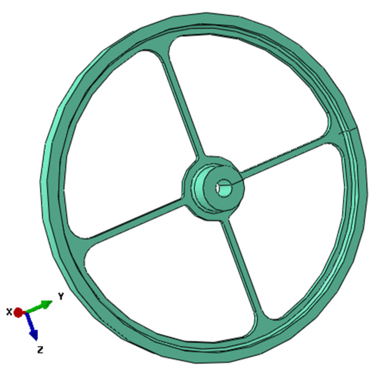
3. Parameterised Finite Element Modelling
The material of the flywheel inertia plate in this work was brass—an isotropic material. Its density, failure strength, elastic modulus, and Poisson ratio are shown in
Table 1.
For the typical working environment of flywheels in engineering applications, the maximum speed and angular acceleration of flywheel are specified in the satellite attitude and orbit control design. The flywheel optimisation provided in this work was based on a case encountered in the project, where the flywheel design requirements stipulated that the maximum speed be 6000° rad/s, and the maximum angular acceleration be 5° rad/s
2. During optimisation, the worst working state of the flywheel was selected for optimisation; that is, the flywheel speed just reached the highest value (6000° rad/s), and the angular acceleration was 5° rad/
(it would change to 0° rad/s
2 at the next moment). At this time, the inertia and rotation of the flywheel produced the largest centrifugal force and the largest stress, and it was closest to its own failure strength, as shown in
Table 2.
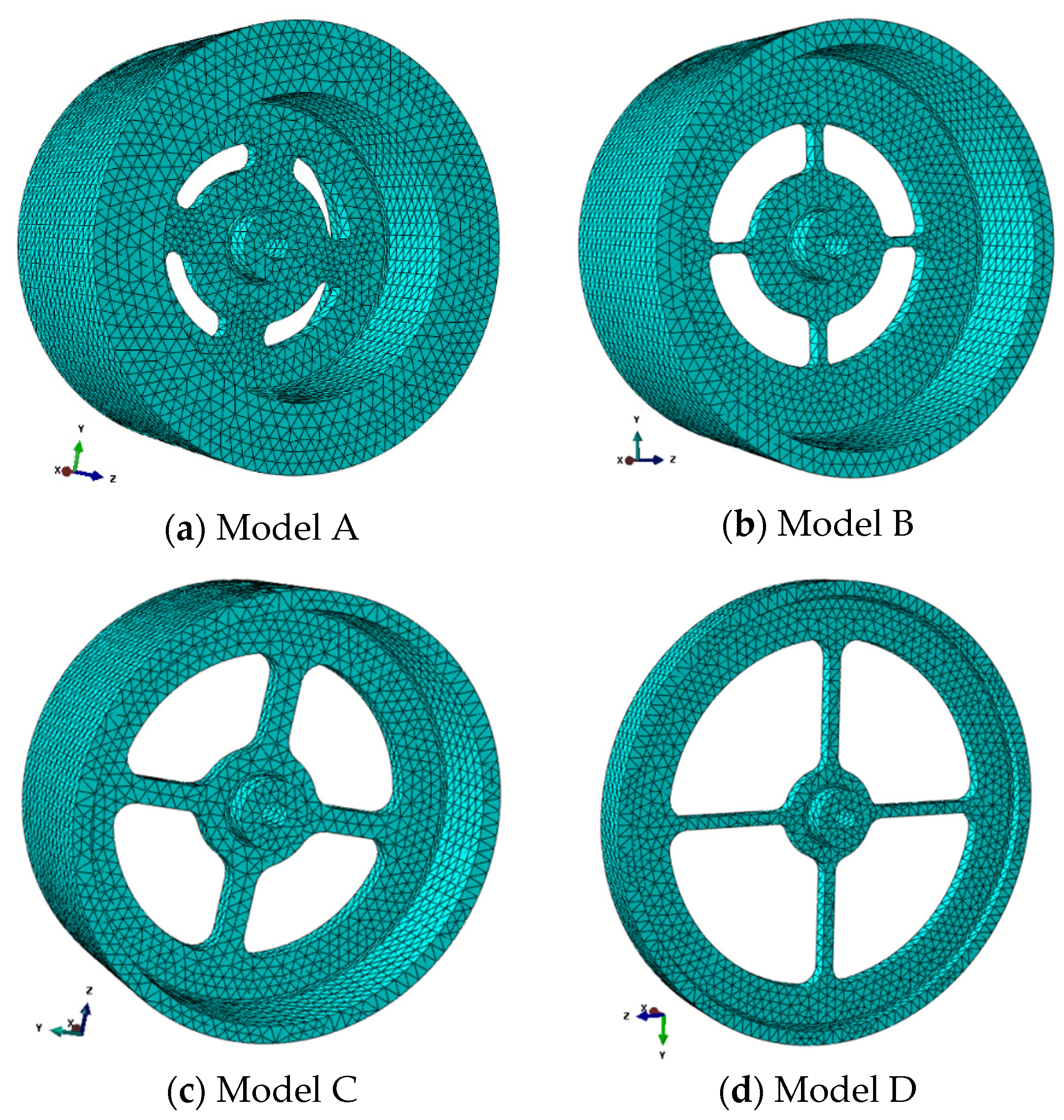
The parametric secondary development of the Abaqus FEM software can achieve the fast modelling of the flywheel model with different structural parameters, including flywheel material, constraints, mesh, etc.
Figure 5 shows the fast modelling of the flywheel FE model with different shape parameters.
The grid type used for the above FE model was C3D10, and the number of grids was 9088. The C3D10 grid is a solid cell grid, suitable for isotropic materials of the metal class.
4. Results and Discussion
4.1. The Effect of the Optimisation Evaluation Factor Re
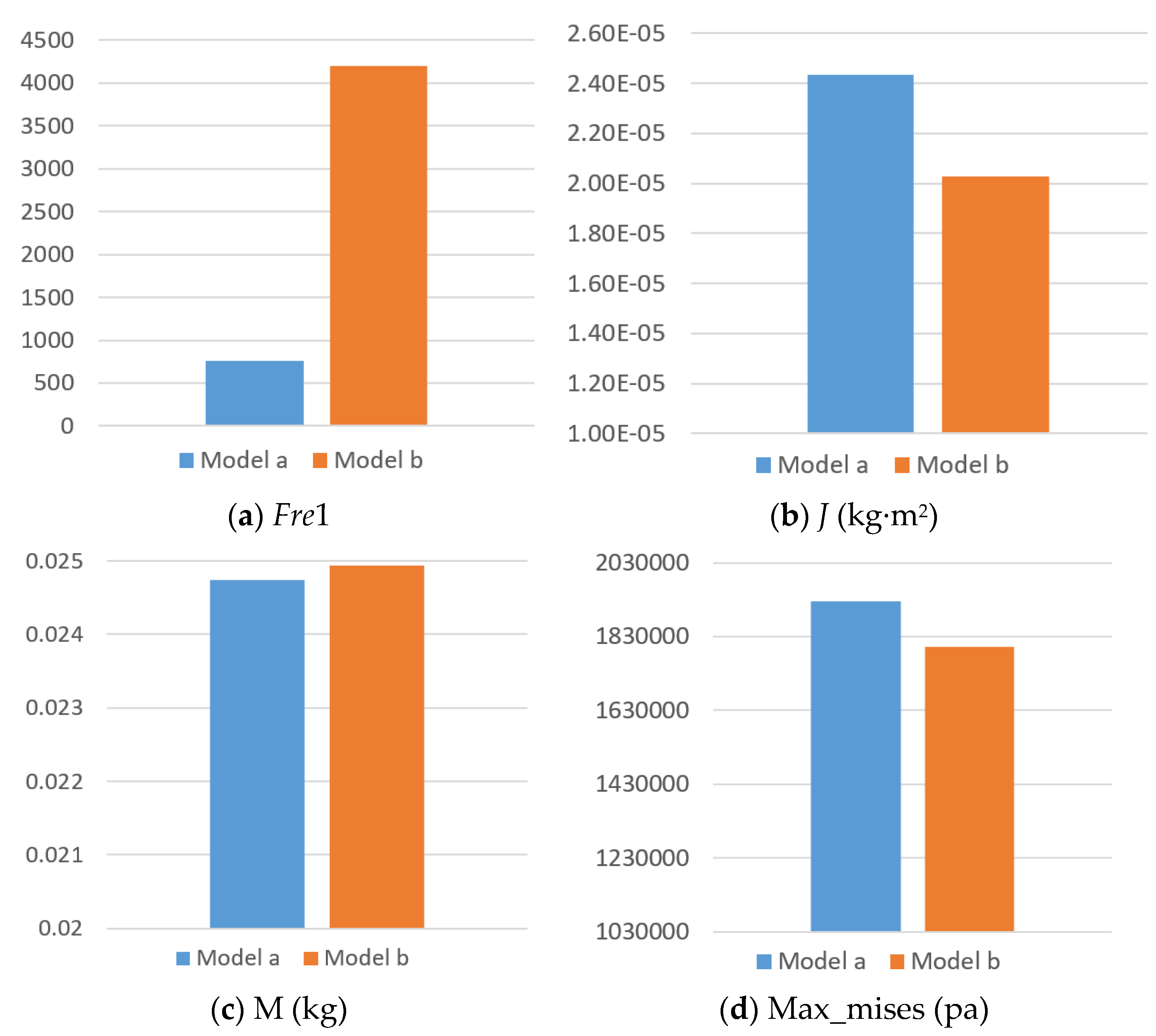
In multi-objective optimisation, the setting of different optimisation objectives affects the final optimisation scheme results and how to weigh the proportion of multi-objective parameters for the final high-performance flywheel inertia disc. This work used the optimisation evaluation factor proposed above as the optimisation balance point. In order to explore the influence of the optimisation evaluation factor on the optimisation results, Optimisation Model A and Optimisation Model B were established in this work. The optimisation objective of Optimisation Model A does not include the optimisation evaluation factor as follows:
The optimisation objective of Optimisation Model B includes the optimisation evaluation factor , as follows:
Other conditions of the two optimisation models—such as constraints, optimisation variables, and optimisation parameter settings—are the same, and the optimisation results are shown in
Figure 6.
Compared with the results of the optimised models, it can be seen that there is little difference in the mass and the maximum Mises stress of Model A and Model B, as shown in
Figure 6c,d, respectively. The first-order vibration frequency of Model A is far less than that of Model B, as shown in
Figure 6a, indicating that the flywheel inertia disc stiffness obtained by the optimisation scheme of Model A is far less than that of Model B. In
Figure 6b, the inertia of Model A is slightly larger than that of Model B. Overall, the optimisation model considering the optimisation evaluation factor Re has a significant impact on the stiffness of the flywheel inertia disc, and a more comprehensive scheme can be obtained in terms of performance.
4.2. Approximate Model
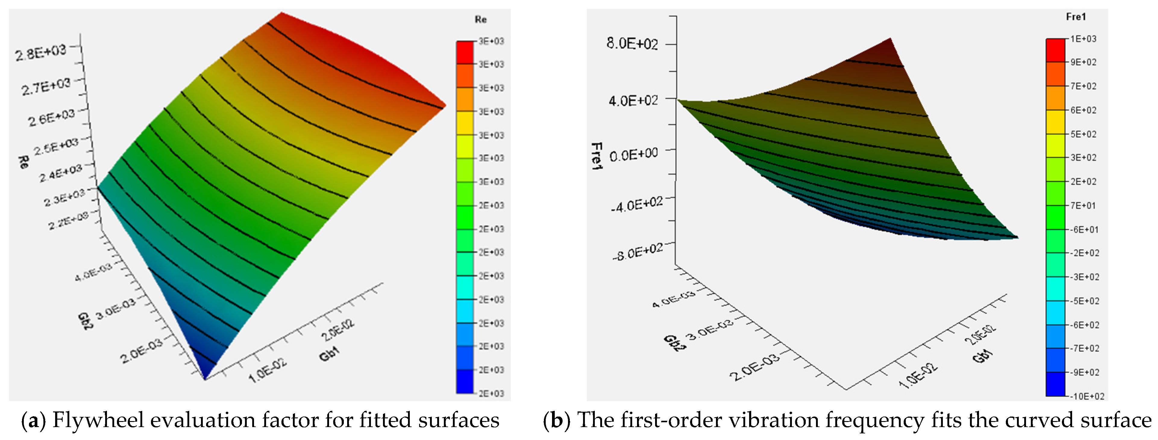
The partial approximate fit surfaces of the flywheel evaluation factor
Re and the flywheel first-order vibration frequency 𝐹𝑟𝑒1 in the optimisation objective are shown in
Figure 7. The R-squared values of the approximated surfaces are 0.998 and 0.985, respectively, indicating that the RBF radial basis fitting model is a very good fit for the flywheel simulation data.
4.3. Initial Optimisation Analysis
This work provides results for four sets of initial optimisation under the same optimisation agent model, as shown in
Table 3.
From the initial optimisation results, the optimisation objectives Re and Fre1 can reach a good level, but the range of optimisation parameter results varies widely between different optimisation groups, which may be due to two reasons: First, the optimisation parameters have a small impact on the optimisation objectives, resulting in a large range of their value distribution from the optimisation results. Second, the range of optimisation parameters is set too large, so the optimisation model cannot effectively find the global optimal solution, and falls into the local optimal results. To address the above problems, the optimisation algorithm can be improved and the model reconstructed using a more widely adapted optimisation algorithm, which requires a longer period of fundamental research, and is not suitable for engineering applications. In addition, the upper and lower limits of the optimisation parameters can be narrowed to reduce the optimisation difficulty. In this work, the optimisation model is re-updated for the upper- and lower-bound intervals of optimisation parameters in the initial optimisation, and the number of populations and genetic generations is increased to achieve the purpose of improving the optimisation model.
4.4. Final Optimisation Result Analysis
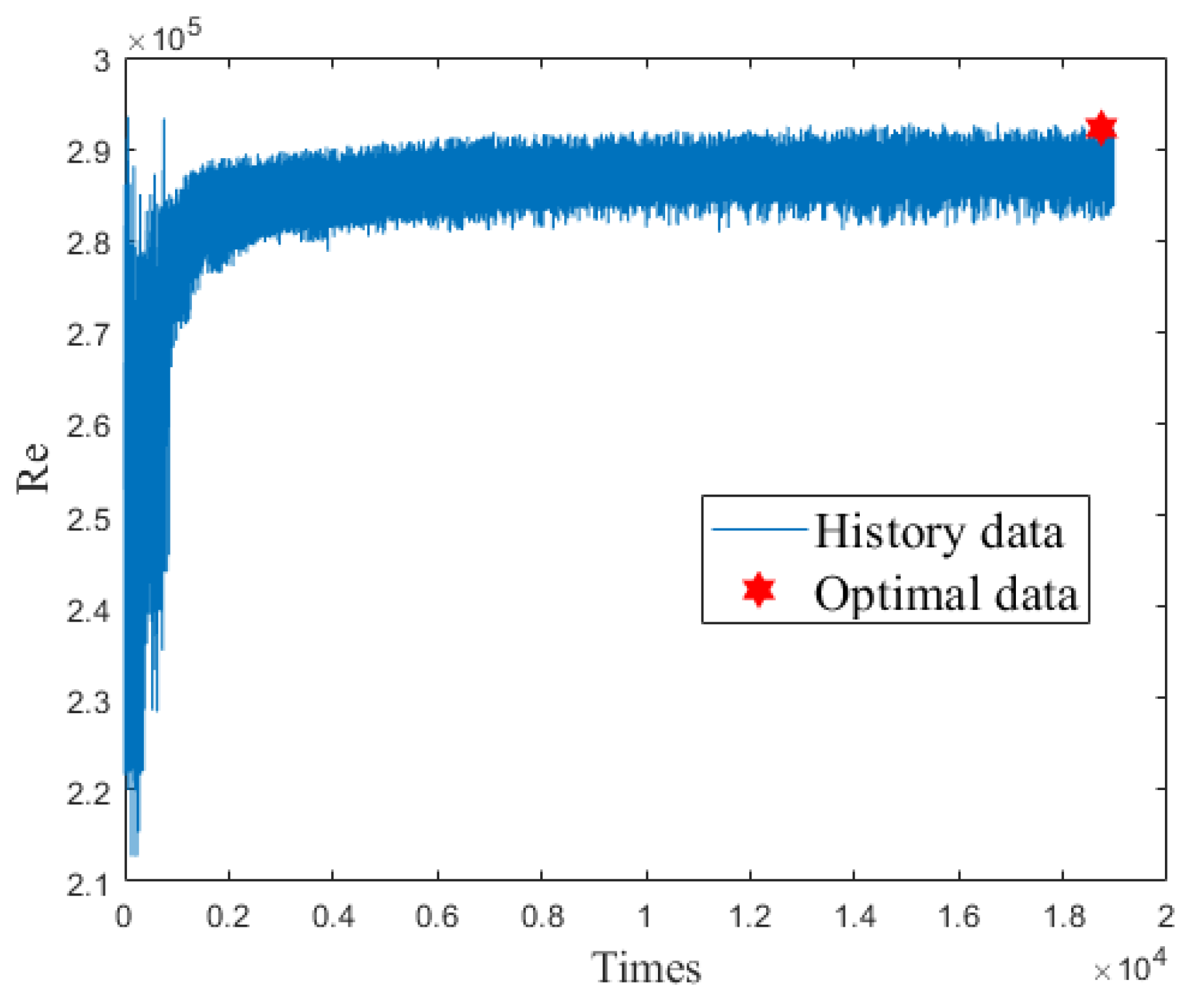
The optimisation results of the improved model are less random, and the optimal size parameters of the flywheel can be obtained, where the population is set to 100 and the genetic generation is 200. The optimisation history curve of the flywheel performance evaluation factor
Re is shown in
Figure 8.
During the optimisation process, the
Re value and the first-order vibration frequency
Fre1 gradually stabilise with the genetic algebra and, finally, arrive near the optimal solution, which is indicated by the red hexagram in
Figure 8. From the stability of the final optimisation value, the number of populations and the genetic algebra are reasonable. The optimised optimisation parameters are replaced into the secondary development model to obtain the shape characteristics of the flywheel in the final optimised state, as shown in
Figure 9.
The final optimised shape shows that the flywheels 𝑋
𝑎, 𝑋
𝑏, and 𝑋
𝑐 are smaller, which can effectively reduce the weight of the flywheel. 𝐽
𝑟1 > 𝐽
𝑟2, which means that the effect of 𝐽
𝑟2 on the flywheel efficiency is smaller than that of 𝐽
𝑟1 when the flywheel is chamfered. The inertia is mainly generated at the periphery of the flywheel, i.e., the size of 𝐺
𝑏1 and 𝐺
𝑏2 is also higher. From the overall optimisation point of view, the effectiveness of the flywheel is ensured by the combined effect of its dimensional parameters, which is also closely related to the optimisation objectives and constraints of the flywheel.
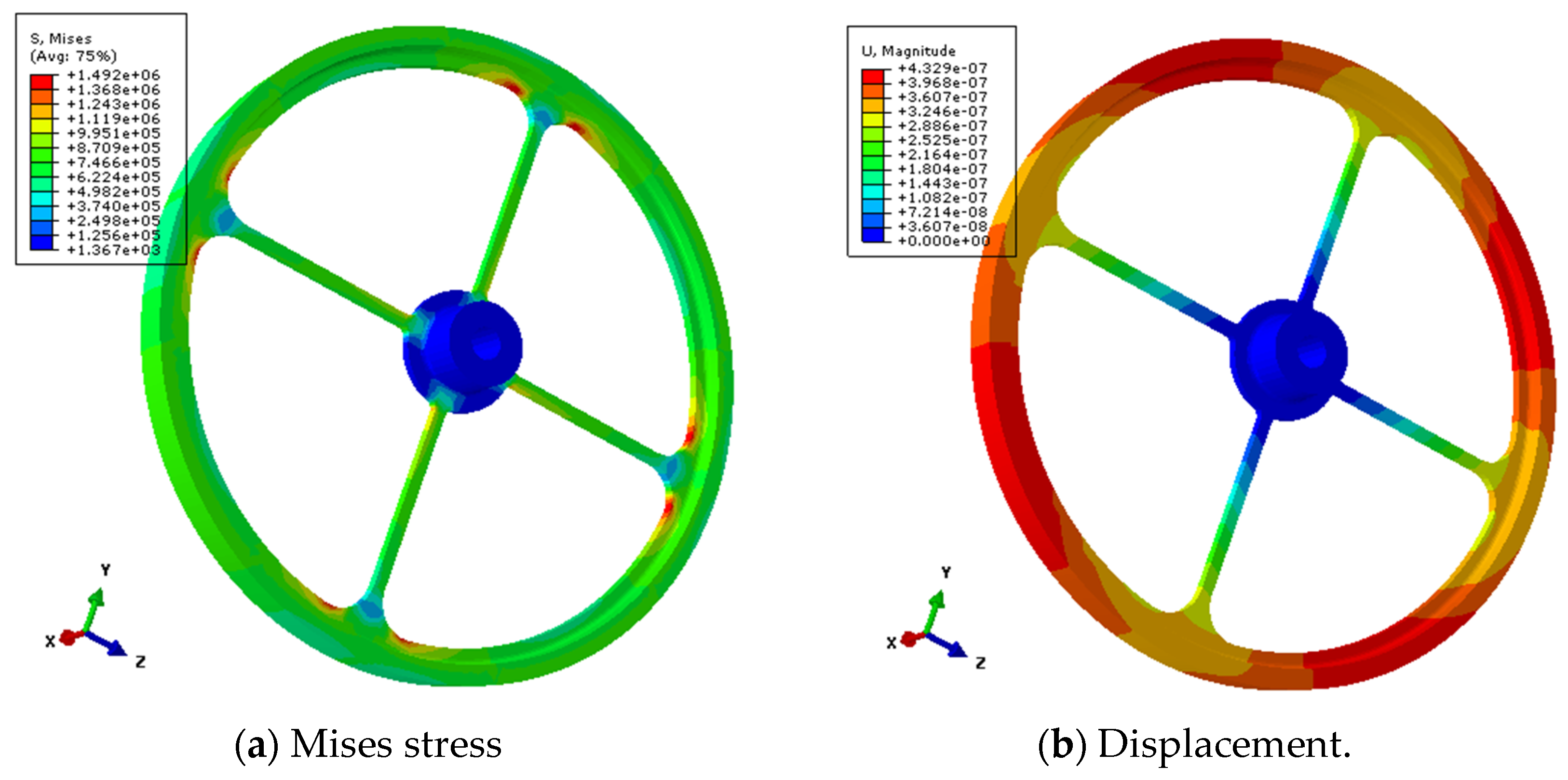
Figure 10 shows the finite element simulation results of the flywheel in the optimal solution state.
Figure 10a shows the Mises stress distribution cloud of the flywheel as a whole in the optimised state, and its overall level is much smaller than the yield stress of the material, so the strength of the flywheel in this state satisfies the demand. In the flywheel’s working condition, the maximum Mises stress generated by the speed and angular acceleration is concentrated on the round corner 𝐽
𝑟1, and the larger 𝐽
𝑟1 can effectively prevent the stress concentration, which is the reason that 𝐽
𝑟1 > 𝐽
𝑟2. The Mises stress level near the centre of the flywheel is lower, but this is the result of not considering the frictional effect of the motor on the centre of the flywheel. In this work, the parameters at the centre of the flywheel are set according to the values of the existing test flywheel, so there is no problem of flywheel root damage, and the parameters at the centre of the flywheel are not optimised parameters.
Figure 10b shows the comprehensive displacement–deformation cloud of the flywheel in the optimal state, where the maximum deformation of the flywheel occurs at the periphery away from the part connection under the action of centrifugal force. The deformation of the flywheel in this state is very small in terms of the deformation magnitude, and no interference caused by the deformation occurs with other parts of the satellite platform.
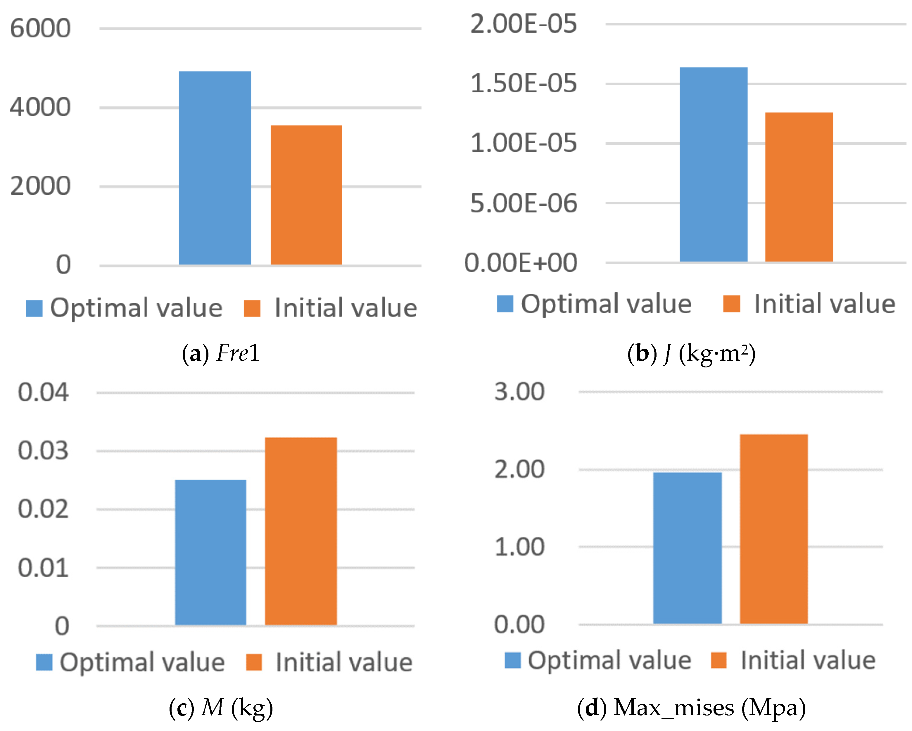
The specific parameters of the optimisation results and the alignment with the initial value are shown in
Figure 11.
In the above figure, the initial values are the relevant data obtained from the simulation under the original flywheel shape parameters. Compared with the initial values, the optimised flywheel has greatly improved performance in all aspects. Under the premise of 22.66% reduction, the inertia increased by nearly 30.16%, the first-order vibration frequency increased by 38.06%, and the maximum Mises stress was reduced by 19.756%. From the perspective of the optimisation effect, the mass of the flywheel inertia plate decreased by 22.66% on the premise of ensuring the improvement of stiffness after optimisation. The maximum Mises stress reduction indicates that the stress distribution is more reasonable, and effectively reduces the risk of flywheel failure. The above results and data show that in practical engineering applications, the appropriate optimised intelligent algorithm to design the flywheel can effectively improve the overall efficiency of the flywheel—especially for micro/nano-satellite platforms, which are particularly sensitive to weight.


