Article

Characterizing an Air-Bearing Testbed for Simulating Spacecraft Dynamics and Control

State Key Laboratory of Mechanics and Control of Mechanical Structures, Nanjing University of Aeronautics and Astronautics, Nanjing 210016, China
*
Author to whom correspondence should be addressed.
Aerospace 2022, 9(5), 246; https://doi.org/10.3390/aerospace9050246
Submission received: 26 March 2022 / Revised: 24 April 2022 / Accepted: 25 April 2022 / Published: 1 May 2022
(This article belongs to the Special Issue Recent Advances in Spacecraft Dynamics and Control)

Abstract

:
Ground-based testbeds play a critical role in developing and testing different methods of spacecraft dynamics and control. To find the dynamic behavior in such an air-bearing testbed, a detailed characterization of the testbed must be provided via systematic testing approaches. This paper describes a planar air-bearing testbed to develop control methods in spacecraft on-orbit operations. This testbed has an almost frictionless surface and can be used to simulate two-dimensional motions in the microgravity environment, with one rotational and two translational degrees of freedom (DOF). The hardware and software architectures of the testbed are presented in detail and key parameters are characterized by a series of systematic test approaches. In addition, a new visual navigation method was designed as an alternative to the external visual system. Finally, two typical case studies are presented to demonstrate the performance of the developed testbed.

1. Introduction

Small satellites are becoming increasingly recognized internationally for their cost-effectiveness as tools for a wide range of on-orbit missions [1]. Thus, the space administrations and governments of some countries have been actively developing small satellite technology for more on-orbit missions in recent decades [2,3,4,5]. The rise of on-orbit scientific missions has led to an increased need for ground-based experiments that are designed to improve the traditionally low success rate of on-orbit missions [6]. Therefore, the demand for a higher success rate depends on the motion system reliability and autonomy performance which are limited by some critical subsystems, such as attitude- and position-control systems (APCS). Currently, performance tests are the primary method of determining key parameters and their relationships to APCS, which is one of the essential measures that can improve the technical level of APCS and is critical to its design and use.
The Spacecraft On-orbit Operation Simulation Testbed (SOOST) at the State Key Laboratory of Mechanics and Control of Mechanical Structures (SKLMCMS) of Nanjing University of Aeronautics and Astronautics (NUAA) was originally developed to simulate and test the dynamics and control of tethered satellites. Researchers at SKLMCMS have extended the design of the testbed to account for small satellites with different functions. SOOST has been in operation and is constantly being upgraded, with four generations of spacecraft simulators having been developed over the past decade. Each simulator generation is designed with a different mission. The first-generation simulator was developed to simulate the deployment and retrieval control of tethered satellite systems, which could weigh more than 80 kg and has a diameter of 0.62 m [7,8]. The second-generation simulators used proportional electromagnetic valves with pressure feedback to enable position control and used momentum wheels to adjust their attitudes [9]. Additionally, each second-generation simulator decreased the mass to 12 kg with a 0.2 m diameter. Third-generation simulators achieved better reliability, maintainability, and usability by markedly simplifying the hardware system structure compared to second-generation simulators [10]. In this study, fourth-generation simulators were used to design a complete mechanical structure with a series of standardized expansion interfaces by taking advantage of both aluminum constructions and polycarbonate structures. More importantly, a real-time embedded system was used to replace the onboard software using the Windows operating system.
Several new simulation scenarios have been verified in the proposed SOOST in the last five years, such as on-orbit assembly, satellite formation flying, and spacecraft docking [11,12,13,14]. To improve APCS reliability and the performance of the spacecraft simulator, a modular design method was used to support a variety of configurations and capabilities in previous studies [15,16]. The SOOST serves as an effective platform to simulate a microgravity orbital environment, although it comes with the disadvantages of scaling down and reducing problem complexity. However, this design still allows research to be performed in a high-fidelity environment that could achieve real-time data computational demands and help to validate the APCS technologies of the spacecraft simulator. Then, a high-quality testing environment with measured characterization data facilitated the performance assessments of the APCS system and direct comparisons with the results from past projects or characterizations. Additionally, each project can leverage the system and process refinements of the testbed as well as its repository of institutional knowledge to ensure that best practices from past research are used and refined over time. Despite some disadvantages that are associated with those technologies, the SOOST can still be used to validate APCS technologies and hardware capabilities such as sensors, actuators, processing units, telecommunication devices, etc.
The SOOST in the NUAA primarily includes a granite air-bearing testbed and spacecraft simulators. Spacecraft simulators are used for ground-based experiments that simulate satellite dynamics and kinematics in various scenarios. The granite testbed here provides a frictionless surface for all spacecraft simulators, allowing the actuators to affect the relevant dynamic changes in two translational DOFs as well as one rotational degree. In the test environment, spacecraft simulators are levitated on a granite table using carbon dioxide (CO2).
In the last five years, nearly all planar air-bearing testbeds have implemented position control using a set of thrusters, and some have augmented their planar testbeds with a full suite of inertial sensors for navigation [17,18,19,20,21,22,23,24]. Based on previous studies, the SOOST was recently equipped with an onboard RGB-D camera that facilitates autonomous navigation under floating conditions without an external visual system. The system can then markedly widen its potential applications to simulate small satellite missions due to its enhanced locomotion and autonomy. To design and evaluate control algorithms for spacecraft close-proximity operations or derive the expected performance for on-orbit systems based on ground testbed results, knowledge of the testbed characteristics is required. The primary purpose of this study is to determine the full set of relevant performance metrics derived from a series of systematic characterization tests, such as the force properties produced by the thruster under simulated floating. In addition, for useful comparisons with similar devices at different labs globally, this article presents a comprehensive description of the relevant performance metrics, uncertainties, and related methodologies. For example, the gas consumption and force produced by the actuator are discussed. This paper also investigates the ability of other similar planar air-bearing devices to replicate the process to evaluate the metrics of their testbeds.
As a typically active three-DOF planar testbed [21], the SOOST is equipped with arrays of cold gas thrusters and an embedded system is used to control the thrusters and onboard sensors. Currently, many similar active three-DOF planar testbeds exist globally. The Small Satellite Dynamics Testbed (SSDT) at Jet Propulsion Laboratory (JPL), is distinguished by its emphasis on traceability during flight and its new thruster system [21,22]. However, there are some errors related to manual operations in the characterization tests that identified key parameters of the SSDT platform, such as variations in the differences in the manual reading of the analog pressure gauge in the single-thruster air consumption test [21]. The Proximity Operation of Spacecraft: Experimental Hardware-in-the-Loop Dynamic simulator (POSEIDYN) developed by the Naval Postgraduate School (NPS) aims to provide a representative system-level testbed upon which to develop, experimentally test, and partially validate control algorithms for rendezvous and proximity operations [17,18,25,26]. However, the performance of the thrusters is characterized by the assumption that the measured force has an equal contribution from any two thrusters in the POSEIDYN. The Kinesthetic Node and Autonomous Table-Top Emulator (KNATTE) developed by Lulea University of Technology (LTU) intends to create a corpus of tests to determine dynamic behavior in a frictionless simulation [23]. Because pressure consistency is not considered in the experimental tests for measuring the thruster forces, the average value differs markedly from thruster to thruster. Other similar testbeds, such as Orbital Robotic Interaction, On-orbit servicing, Navigation (ORION) [24], the Platform Integrating Navigation and Orbital Control Capabilities Hosting Intelligence Onboard (PINOCCHIO) [19,20,27,28], the Synchronized Position Hold Engage and Reorient Experimental Satellites (SPHERES) [29,30], and Complex for Satellites Motion Simulation (COSMOS) [31], do not provide a detailed characterization of their testbeds for systematic test approaches.
Thus, the SOOST is characterized by user-customizable, systematic test means, a detailed characterization of the system, its relatively complete sensor system, a lower system latency, and its modular design that supports a wide variety of applications. For example, a user can choose the force magnitude produced by thrusters based on a real payload mass or other requirements. From an experimental standpoint, the SOOST planar system offers great flexibility and independence by the adoption of an onboard CO2 tank and battery.
This paper is organized as follows. Section 2 provides a detailed description of the design of the SOOST’s hardware architecture, including the mechanical subsystem, the electric subsystem, and the pneumatic subsystem. In Section 3, the testbed system software architecture is discussed in detail. Section 4 presents the performance characterization testing conducted in the SOOST and the resulting relevant performance data as a basis for systematic comparisons with other similar testbeds and research. Two typical case studies are completed to assess the capabilities of the SOOST in Section 5. Finally, Section 6 provides conclusions and future study directions of this field of research.

2. Hardware Architecture of Testbed System

This section presents a detailed description of the hardware architecture of the SOOST, with an emphasis on the pneumatic subsystem. The pneumatic subsystem is designed to acquire two critical capabilities to create an almost frictionless environment and supply the actuators to achieve position control. Even though there are many similar studies in the literature, the design concept provided in this section is focused on the practicality principle of the devices.

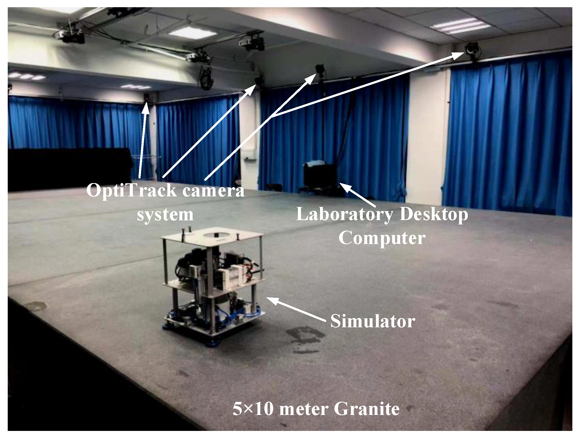
2.1. Hardware Overview

The SOOST planar testbed system is composed of the following three primary elements: a 5 × 10 m2 granite platform, multiple spacecraft simulators, and a laboratory-scale motion capture system (OptiTrack camera system). An overview of each of these elements is shown in Figure 1.
The entire 5 × 10 m2 granite platform is made of four smaller pieces of 5 × 2.5 m2 granite. Every small piece of granite is supported by a set of adjustable pedestals that allow the granite surface to be horizontally leveled to an accuracy of 0.005 deg. The subsided foundations and some building structural activities could cause the entire granite surface to tilt over time; thus, periodic measurements are required to ensure that the surface is level to within the preset tolerance.
Spacecraft simulators are custom-designed vehicles that simulate spacecraft orbital dynamics. In this study, fourth-generation spacecraft simulators are used. An almost frictionless and microgravity environment is established using the gas discharged from three flat 50-mm-diameter air bearings to generate an approximately 5 μm thick air film between the granite surface and the spacecraft simulator. The air film acts as a lubricant film, which eliminates direct contact between the granite surface and the simulator. Therefore, the planar motion simulates flight-like dynamic behaviors. Compared with the 6-DOF motion of an on-orbit spacecraft, the SOOST only allows 3-DOF motion (two translations and one rotation), which is a critical physical limitation of the testbed. However, the testbed can still simulate many important functions in space system development in many situations and is intuitive to use.
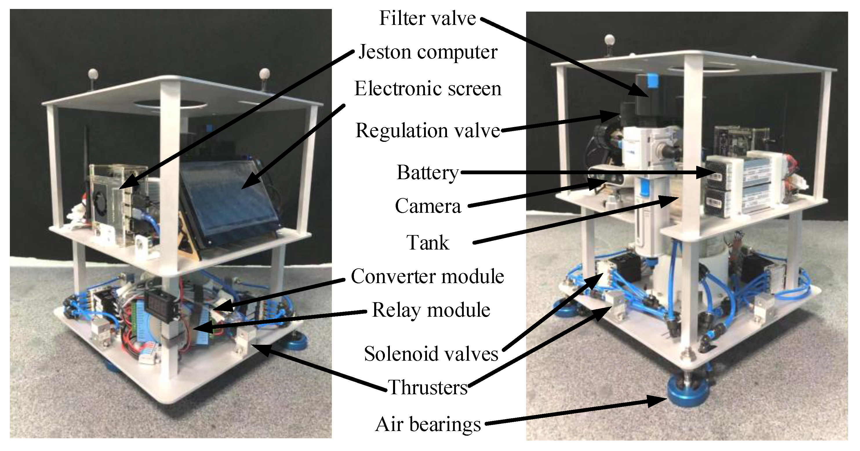
As shown in Figure 2, the simulator primarily consists of four subsystems which are as follows: the mechanical subsystem, the electronic subsystem, the pneumatic subsystem, and the payload subsystem. First, the mechanical subsystem rigidly supports all subassemblies together using custom-designed aluminum plates and polycarbonate fasteners. Then, from top to bottom, the electronic subsystem contains an embedded computer, a power supply, an electronic screen, a wireless communication module, a serial converter module, and a relay module. Third, the pneumatic subsystem is primarily composed of a CO2 tank, a pressure regulation valve, a filter valve, eight solenoid valves, eight thrusters, and three air bearings. Finally, the payload subsystem is an optional subsystem that may include additional sensors (e.g., IMUs), an RGB-D camera, additional actuators (e.g., reaction wheels), or special equipment (e.g., robotic manipulators, docking mechanisms).
In different simulated missions, the simulator is configured to include all required subsystems while removing unrequired subassemblies so as to reduce mass. Thus, the mass and inertia of the system vary with different test campaigns. When the payload subsystem is not considered, the mass of the system ranges from approximately 9.6 kg to 10.4 kg, the inertia perpendicular to the surface is approximately 0.1445 kg·m2, and the center of mass tends to be located within 6 mm of the geometric center on the surface. A more detailed description of this configuration is provided in Section 4.
The SOOST’s laboratory-scale motion capture system is a commercial system (OptiTrack) that includes eight PrimeX 41 cameras, four PrimeX 22 cameras, and an external computer. The field of view of the motion capture system covers the entire granite surface. Additionally, the OptiTrack camera system can provide better performance for three-dimensional reconstruction in real-time. Additionally, this system can measure the position and orientation of the simulator, which carries passive fluorescent markers with a submillimeter-level accuracy at rates of up to 300 Hz.

2.2. Mechanical Subsystem

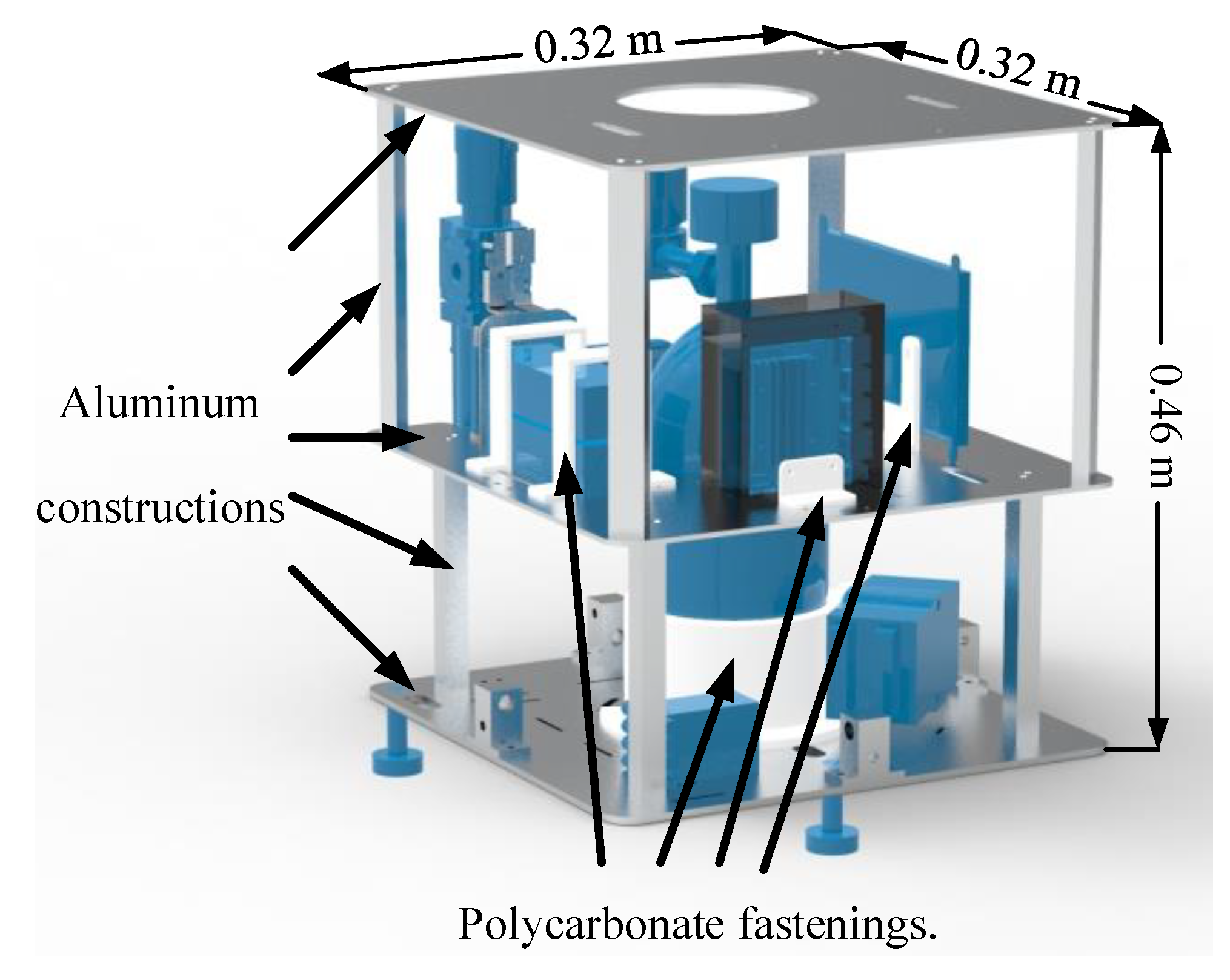
The mechanical subsystem rigidly supports all subassemblies together by taking advantage of both aluminum constructions and polycarbonate structures. The entire structure is a 0.32 × 0.32 × 0.46 m container framework, as shown in Figure 3, which primarily includes three aluminum plates, eight aluminum columns, and some polycarbonate fastenings. The benefit of this system is that it successfully combines the high strength of aluminum and the low mass of polycarbonate. The three aluminum plates provide many attachment points to attach nearly all separate components. Two levels are divided by the three aluminum plates. The level closest to the granite surface holds most of the pneumatic components and a smaller portion of the electronic components, and the upper level is the opposite. The tank crosses through both volumes because the CO2 tank must be upright to avoid self-freezing when exhausting. For the convenience of CO2 tank installation and uninstallation, a circular hole in the roof of the framework is drilled. The payload subsystem could be installed above the framework for dedicated scenarios, and the structure can also expand vertically to obtain additional space if necessary. Additionally, some appendages, such as docking mechanisms and flexible antenna systems, could be attached to the side of the framework using appropriate mounting holes and fastenings.

2.3. Electronic Subsystem

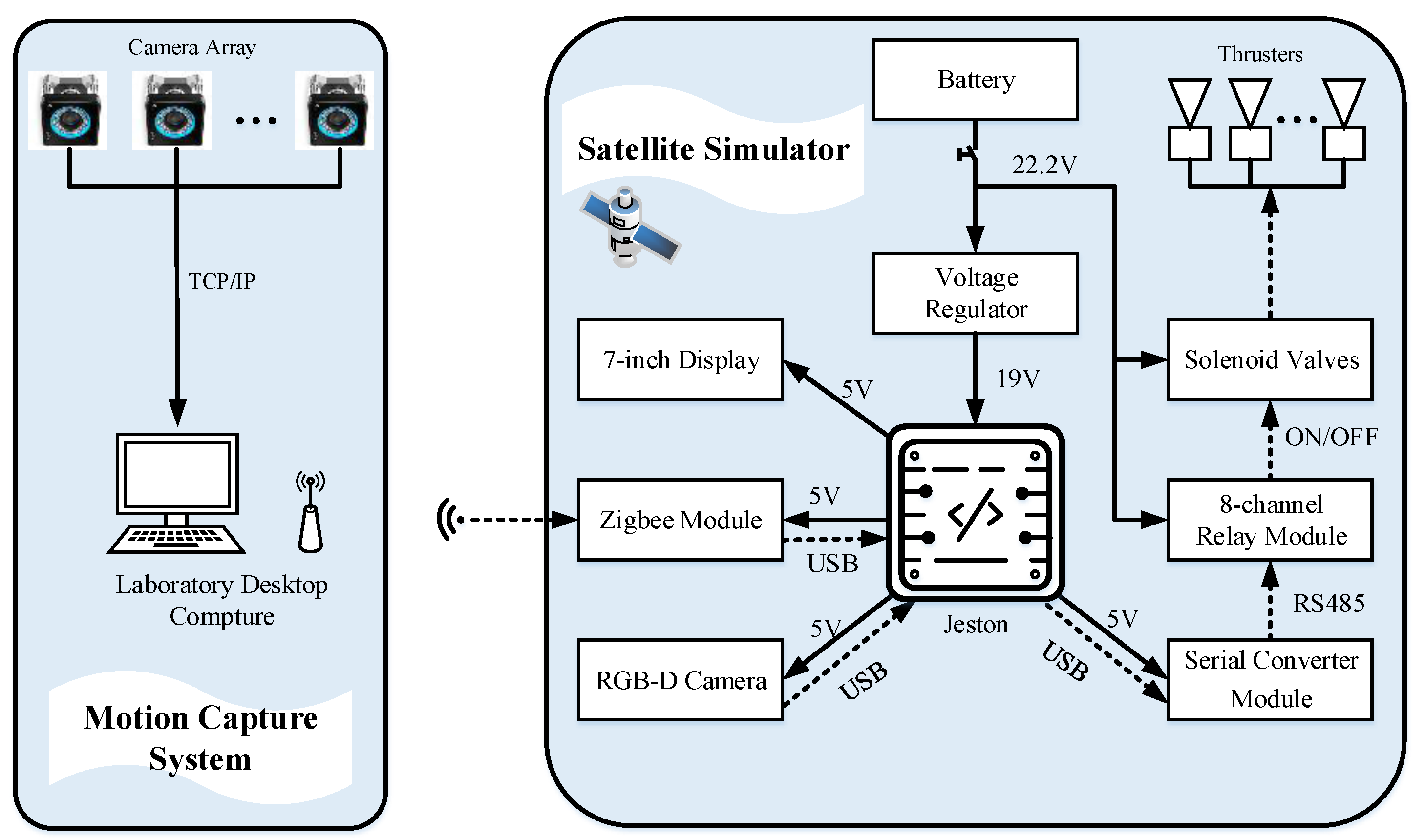
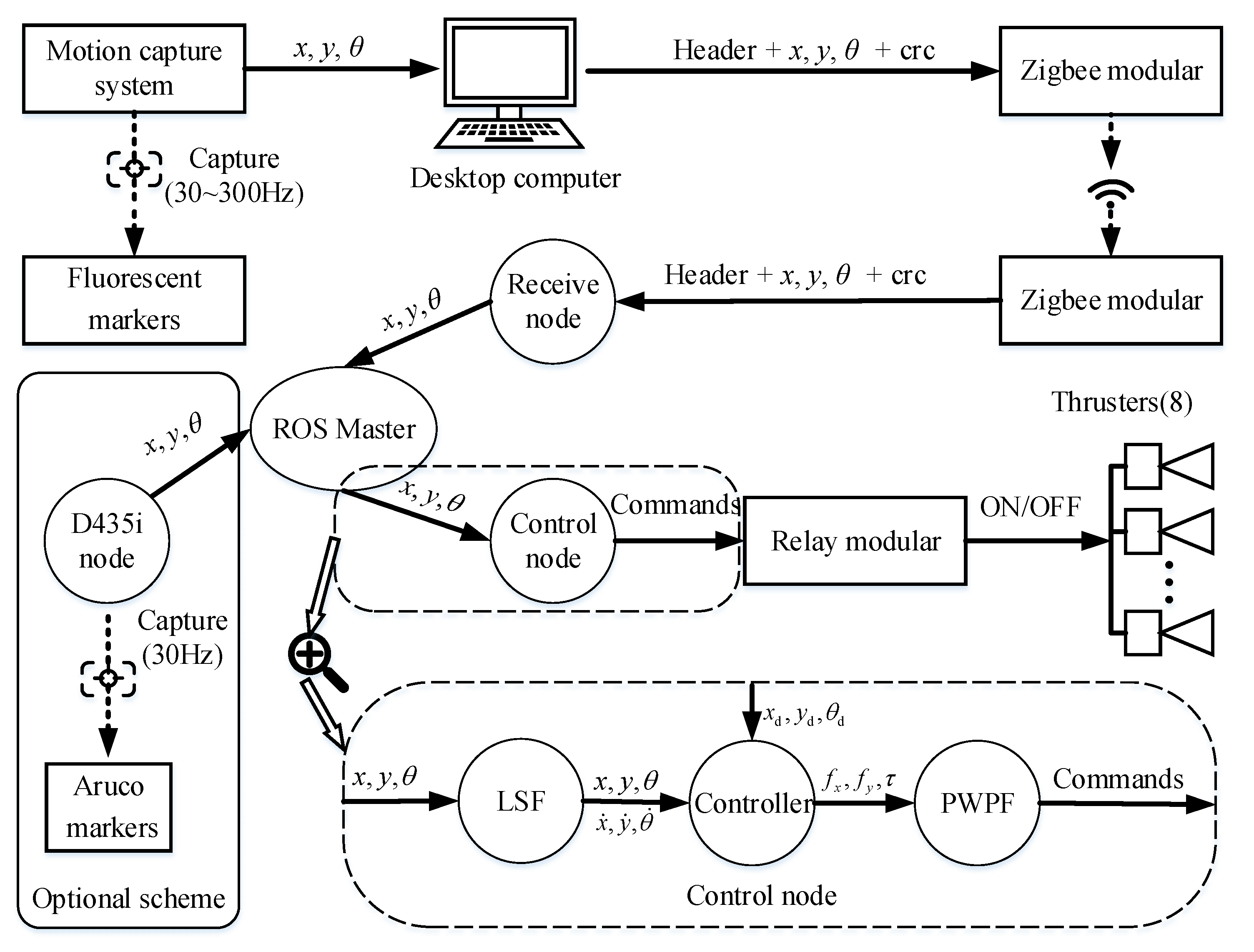
The electronic subsystem is designed to provide a power supply, data processing, and data transmission. The entire electronic subsystem is powered by a power supply system that consists of two 22.2 V Li-Po batteries and a DC voltage regulator. The power supply system has a capacity of 6400 mAh, and the voltage regulator can deliver a steady predictable current through its 19 V output. The core of the electronic subsystem is an onboard Jeston Xavier NX computer running Ubuntu 18.04 LTS, which receives data from sensors and sends the appropriate commands to the actuators. In addition, based on 384 NVIDIA CUDA® Cores, 48 Tensor Cores, 6 Carmel ARM CPUs, and two NVIDIA Deep Learning Accelerators engines, the Jeston Xavier NX provides all of the onboard computational capabilities of the spacecraft simulator.
The Jeston Xavier NX is equipped with four USB 3.0 ports that are occupied by other key electronic components. The first port is occupied by a 7-inch display screen to help to easily debug programs and display the system status. The second USB interface connects a serial converter module to provide one additional high-speed RS-485 port. Then, to ensure that timings are uniform between thrusters when opening or closing more than one thruster at a time, the RS-485 port can communicate with a relay module, which has eight channels to provide the required switching capability for all eight thrusters. Thrusters are opened or closed by the corresponding solenoid valves via the RS-485 port, and the status of each thruster is independently controlled by the Jeston computer. All eight solenoid valves are also powered directly from the power supply system. According to the datasheet, the switching time-on and -off times of the solenoid valve in the new condition are 0.8 ms and 0.4 ms, respectively. Additionally, the typical relay on time and the typical relay off time of the relay module are 3 ms and 4 ms, respectively, according to the product manual. The third USB port is used to communicate with a D435i camera, which combines the robust depth-sensing capabilities of a D435 with the addition of an inertial measurement unit (IMU). The last USB port is connected to a ZigBee wireless communication module, which enables the simulator to communicate with other simulators or the external desktop computer. Compared to the Wi-Fi module used by Ref. [32], the ZigBee module has a lower power consumption and requires a smaller battery capacity, yielding longer use.
The electrical supply and signal block diagram of the testbed is shown in Figure 4, and the electrical properties of the key components are shown in Table 1. Data transmission is denoted with broken lines in Figure 4. Under normal conditions, the power supply system can power the simulator for over 3 h; thus, the amount of CO2 inside the onboard tank is the primary limiting factor during various tests.

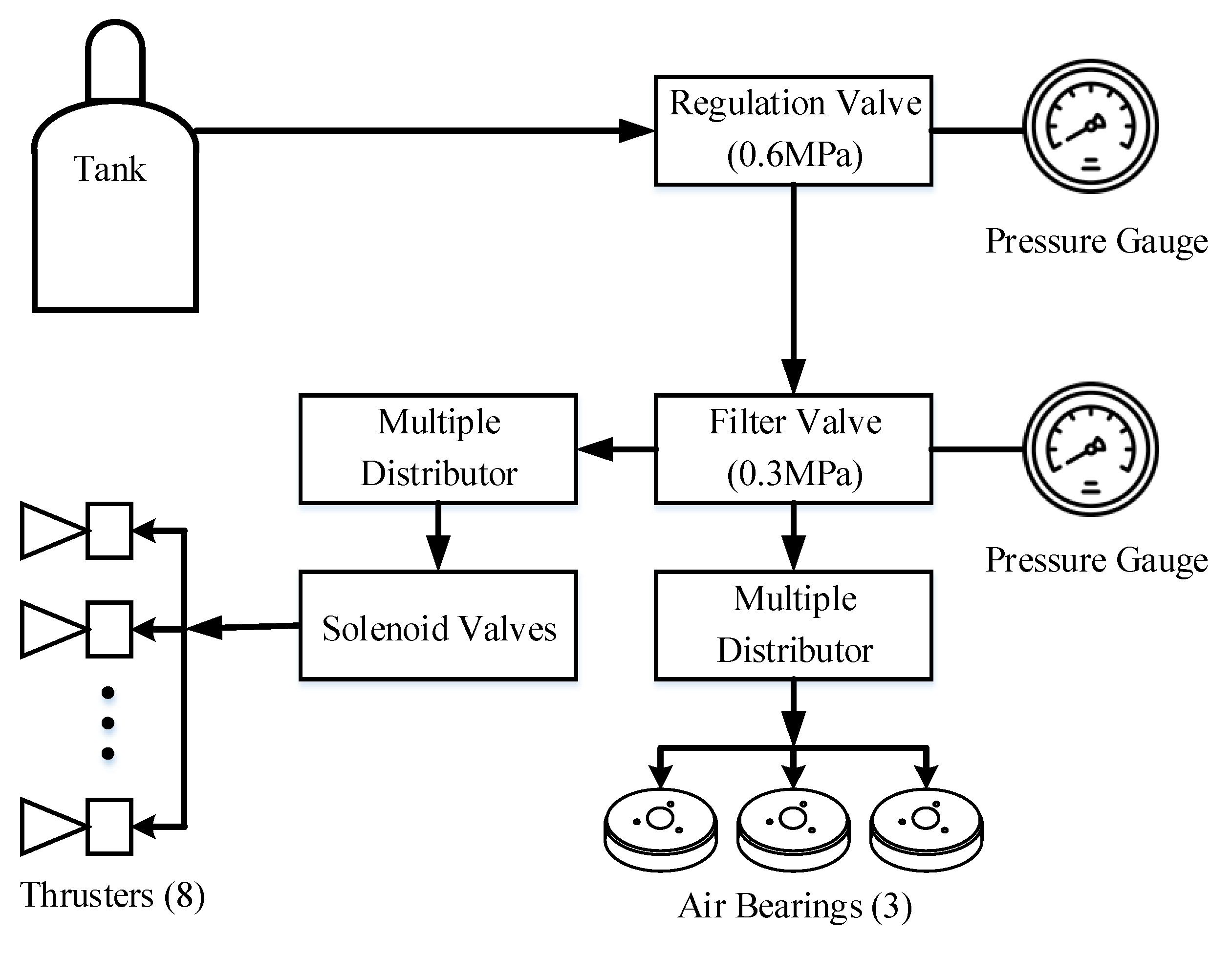
2.4. Pneumatic Subsystem

The pneumatic subsystem plays a critical role in the entire system, and its primary function is to provide the gas supply to the thrusters and the air bearings of the simulator. Due to safety reasons and the high cost of high-pressure gas canisters, CO2 is used in this pneumatic subsystem [33]. The pneumatic subsystem diagram is shown in Figure 5, and its relevant properties are listed in Table 2. A 1.1 L tank can typically store 0.8 kg of CO2 at room temperature and can be disassembled to check the remaining gas supply due to the special structural design. The nominal pressure of the tank is approximately 7 MPa. After flowing through the pressure regulation valve, the CO2 pressure markedly decreases to 0.6 MPa, but the pressure here becomes unstable when switching the thrusters on or off. Thus, a filter valve is used to stabilize the pressure and prevent impurities in the CO2 from damaging the delicate air-bearing porous material. Then, the CO2 is divided into two pipes with the same pressure which can be regulated as follows: one pipe is directly connected to the three air bearings to lift the simulator and make it float above the granite surface using three air bearings that are mounted to the bottom of the simulator in an equilateral distribution; and another pipe travels through the solenoid valves to supply the thrusters.
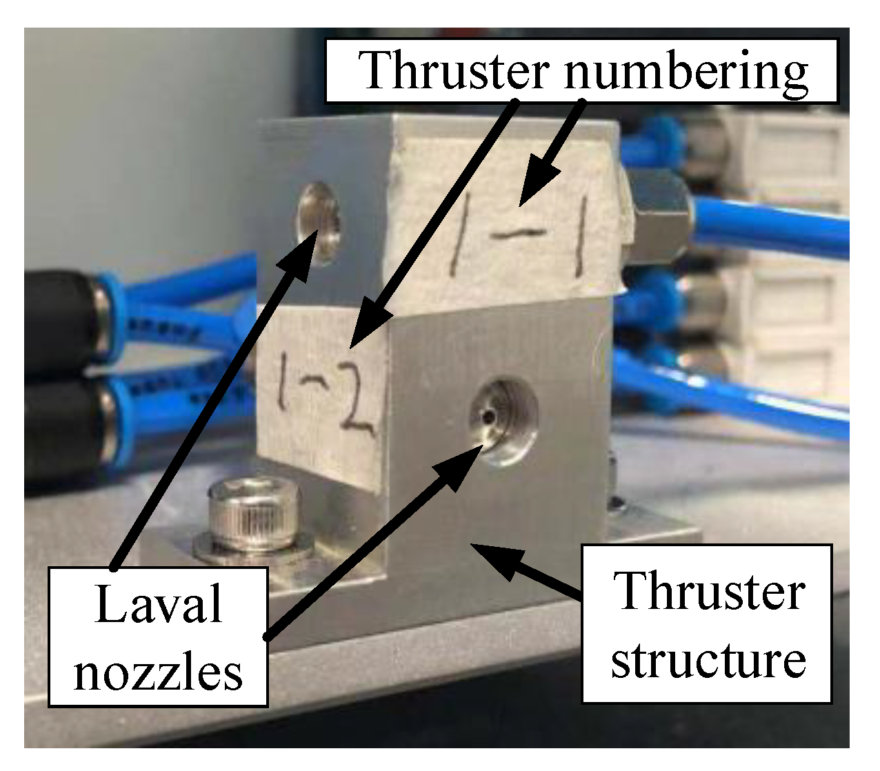
These thrusters could be divided into two parts (four normal cases and four tangential cases) to control positive and negative translations in the x b -body and y b -body axes, and the rotation about the z b -body axis, respectively. Each thruster structure is allocated at the edges of the simulator, which is composed of one normal case and one tangential case. As shown in Figure 6, two Laval nozzles [34,35] are embedded into one thruster structure. 
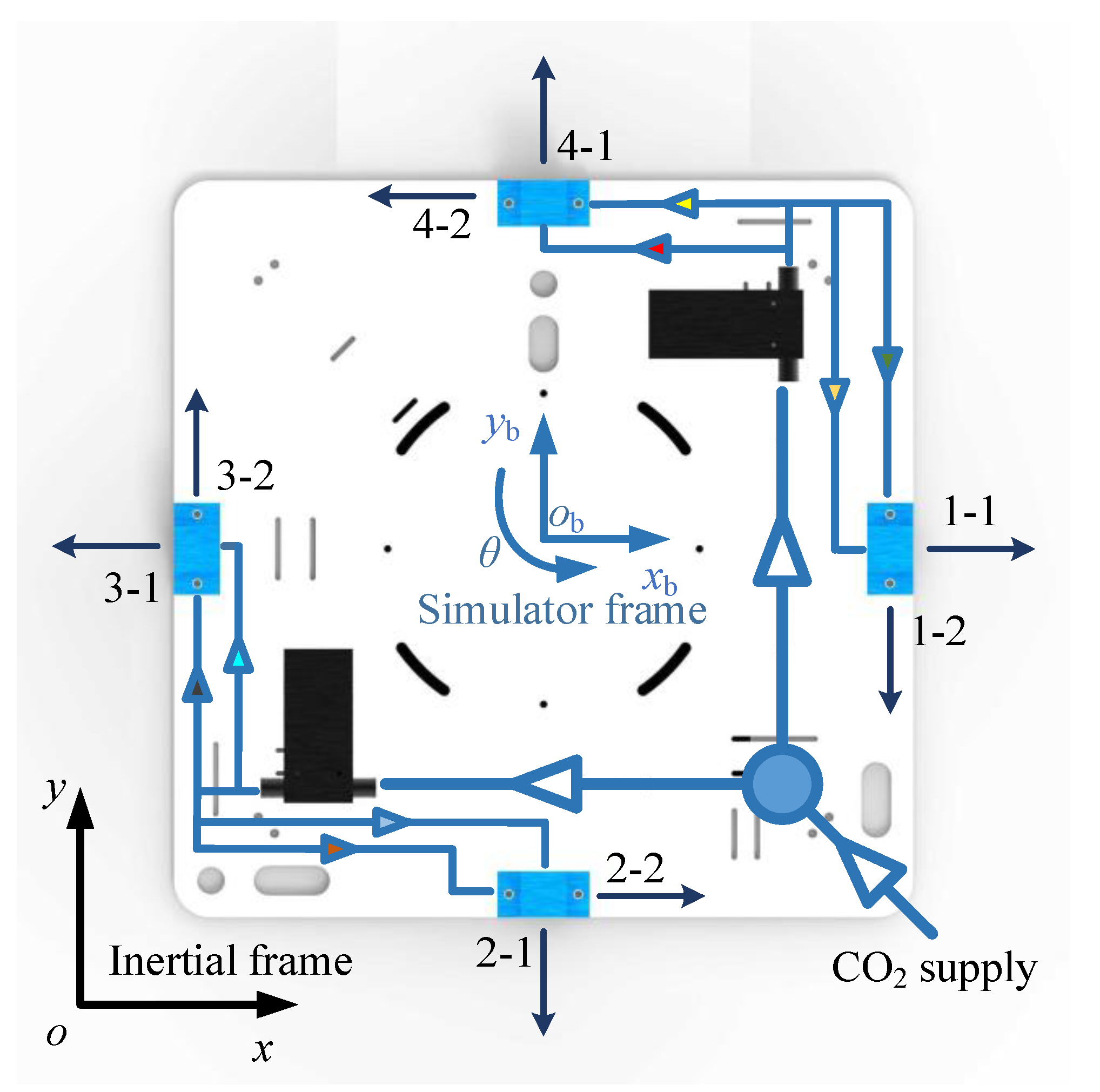
Figure 7 shows the thruster numbering convention used by the control law, where the coordinate systems of the simulator and inertial frames are defined, and the directions of the exhausted forces are represented by arrows.

3. Software Architecture of Testbed System

This section describes the software architecture of the simulator in detail. The primary components of the software include the thruster control strategy and the autonomous visual navigation method. Based on the ROS ecosystem, the entire software architecture is built using a set of functional ROS nodes. Thus, the software presented in this section can be easily coded in this architecture.

3.1. Software Overview

This section describes the software architecture for onboard control systems in detail. Because this spacecraft simulator is expected to become more practical, the onboard system is required to manage two key issues, which are as follows: obtaining the expected real-time property and remaining integrated with other testbeds. To address the first issue, the onboard Jeston Xavier NX computer hosts the developed software based on a 64-bit Ubuntu 18.04 operating system, and its Linux kernel has been patched with the real-time-Preempt patch [36]. The other issue is resolved via the robot operating system (ROS) which provides many features in the form of ROS nodes and facilitates rich communication between them in a peer-to-peer fashion [37], which is a powerful tool in a large runtime system. The real-time capability will be discussed in Section 4 in detail.
The desired workflow was achieved using the software architecture shown in Figure 8. The circles and rectangles in the graph represent the software and the hardware, respectively. The current core function of the developed software is to provide data receiving, instruction generation, and data recording.
As shown in Figure 8, the positions of the fluorescent markers are captured in real-time at rates from 30 to 300 Hz using the OptiTrack system that is mounted on the ceiling. Then, the desktop computer is able to determine the three-dimensional coordinates of the simulators. After this, the cyclic redundancy check (CRC) algorithm [38] is used to check the receiver to determine whether the information was received correctly. When a frame packet is encapsulated into a binary number, which includes a given data header and a CRC check code, it is sent to the onboard computer mounted on the simulators via ZigBee wireless communication. Following this, the Receive node within the ROS software framework is used to detect the received data, check the check code, and extract and publish the valid data sequentially. Then, any ROS node can obtain the position data of the simulators from ROS Master.
The Controller node is highlighted in this section. First, a modified least square fitting (LSF) method [39] is used to estimate the velocity data of the simulators. Then, the obtained data are compared with the desired position and the attitude inputs from either a reference trajectory or from a user-defined command to determine the position and attitude error. The error is then used by the designed controller to calculate the force and torque required with regard to the simulator to reach the desired state. Due to the difference between the binary nature of the thruster force and the continuous original command signal, the pulse width/pulse frequency (PWPF) method is used to convert the continuous signal to a switch signal while producing the same overall effect. Finally, the commands generated by the Controller node are sent to the relay module to control the thrusters. Additionally, an optional vision measurement scheme is provided by the D435i node, and a D435i camera is used to capture the external targets to acquire the position of the targets without an external visual system. The remainder of this section will describe thruster mapping and modulation, the modified LSF method, and the vision navigation algorithm.

3.2. Thruster Control Strategy

The thruster control strategy of the simulator includes velocity estimation, thruster mapping, and thruster modulation methods. Only the position information of the simulator can be obtained using the motion capture system; therefore, an appropriate velocity estimation method is required to estimate the real-time velocity information using the recorded position and time data. The prime objective of thruster mapping is to enable the appropriate thrusters to achieve the desired control input, which consists of control forces and torque. Because thrusters can only take on two discrete states (on or off), while the original control signal from the control laws is continuous, a thruster modulation method is required.

3.2.1. LSF Velocity Estimator

Considering the effect of the measurement noise and fixed-time interval sampling, a modified LSF method is proposed to estimate the velocity data of the simulators. Compared to the Kalman filter, the modified LSF method is simpler and more stable. The modified LSF method is described below. First, an N-order polynomial is given by
λ ^ σ k , c = c 0 + c 1 σ k + c 2 σ k 2 + + c N σ k N
which is adapted to fit sampling data σ k , λ k at the nearest sampling point at length M, where σ k is the sampling time, λ k is position data at the time σ k , 1 k M is the sequence number of raw data sampling, k = M is the current sampling time, and c = c 0 , c 1 , c N T is an N + 1 dimension undetermined coefficient vector. Then, the coefficient vector c must be determined to minimize the value of the following formula:
k = 1 M λ ^ σ k , c λ k 2
Once c is determined, an estimate of the current velocity can be obtained using the first derivative with respect to the time of Equation (1) as
λ ˙ σ k = d λ ^ d σ = c 1 + 2 c 2 σ k + + N c N σ k N 1
For the convenience of calculating c, the sampling interval is assumed to be a dimensionless constant whose value is 1, σ k σ k 1 = 1 , where least square fitting is independent of the starting point of sampling. Then, we let σ k = k , where the general solution of LSF is used to derive c as follows
c = A T A 1 A T λ
where λ = λ 1 , λ 1 λ M T , A M × N + 1 and A i j = i j 1 i = 1 , , M ; j = 1 , , N + 1 . Combining Equations (3) and (4), a dimensionless estimate of velocity at σ k is obtained. Additionally, a real value is obtained by dividing the real sampling interval.

3.2.2. Thruster Mapping

As shown in Figure 7, thruster 1-1 is selected to produce the force along the positive direction of the x b -axis. Then, thruster 3-1 is selected to produce the opposite force. A similar situation also exists in thrusters 4-1 and 2-1 along the y b -axis. Then, thrusters 1-2 and 3-2 are opened or closed concurrently to produce a torque around the z b -axis in a clockwise direction, and then, thrusters 2-2 and 4-2 produce the opposite torque.
To project the desired forces and torque in the inertial coordinate system into the local body-fixed coordinate system for the simulator, Equation (5) is recommended as follows:
u = M f
where u = f x , f y , τ T are the desired forces and torque in body-fixed coordinates, f = F x , F y , F θ T are the force produced by the control law, and M 3 × 3 is the mapping matrix, which is given by
M = cos θ sin θ 0 sin θ cos θ 0 0 0 1

3.2.3. PWPF Modulator

Once the requested control force is assigned to the specific thrusters, a modulation scheme can be used to realize the discrete force. Some common pulse modulators have been used to modulate spacecraft actuators, such as PWPF modulators, derived-rate modulators, and pulse-width modulators (PWMs). Among these modulation methods, the PWPF modulator has several advantages, such as a nearly linear operation and high accuracy, and is thus well suited to modulating spacecraft actuators [40,41].
As shown in Figure 9, a typical PWPF modulator is composed of a Schmidt trigger (ST), a prefilter, and a feedback loop. An ST is simply an ON/OFF relay with a dead zone and hysteresis; thus, when the positive input to the ST is greater than Eon, the ST output is Um, and when the positive input is less than Eoff, the ST output is zero. This response is also reflected in negative inputs. Then, the difference between the system input r(t) and the ST output Um is considered the error signal e(t). The error is used by the prefilter, whose output f(t) is used by the ST. The important parameters of the PWPF modulator are the prefilter parameters Km and Tm, and the ST coefficients Eon, Eoff, and Um.

3.3. Visual Navigation Method

To provide autonomous navigation under floating conditions without an external visual system, a D435i camera is mounted onto the simulator. Considering the computing performance of the onboard computer and the vibration caused by the thrusters, a fast, accurate, and robust image processing method is required. Ref. [42] proposed a method for tracking square markers using a set of discriminative correlation filters (DCFs). A DCF-based tracker has high accuracy in estimating the exact location of the marker corners but has poor performance in calculating marker attitude. Thus, a modified DCF-based method was presented to improve the pose recognition performance.
First, to track a square marker continuously along a video sequence, this method uses the following five grayscale filters: one for tracking the marker’s appearance, and four for tracking the four corners. In addition, the subpixel refinement method [43] is used to find the pixel coordinates of the four corners with subpixel accuracy.
Then, a new marker array that includes four markers was designed to replace the original marker, as shown in Figure 10. The marker array can be split into two parts, where the first part includes two markers on the left and the second part consists of the right side. The following three coordinate systems are employed for pose recognition: the marker array frame o m x m y m z m , the left local frame o 1 m x 1 m y 1 m z 1 m , and the right local frame o 2 m x 2 m y 2 m z 2 m . When the marker parameters d gap and d size are known, the coordinates of sixteen corners in the marker array frame o m x m y m z m can be found. We define these coordinates as ξ n m 3 , n = 1 , 2 , , 16 . The coordinates of sixteen corners in the camera frame o c x c y c z c can be defined as ξ n c 3 , n = 1 , 2 , , 16 .
Finally, the EPnP method [44] can be used to estimate the pose of the marker array relative to the camera referential. The central idea of this method is to express ξ n m as a weighted sum of four virtual control points. The pose estimation problem is then reduced to estimate the coordinates of these control points in the camera reference, which can be completed by solving a constant number of quadratic equations to choose the best weights.

4. Testbed System Characterization

This section describes the characterization of the SOOST planar testbed and primarily focuses on the center of mass, single-thruster force, multiple-thruster force, the moment of inertia, float duration, single-thruster CO2 consumption, multiple-thruster CO2 consumption, and system latency. A series of tests were then performed to describe these characteristics under different testing conditions, principally the pressure of the supply CO2. Test data can be used for a systematic comparison of the capabilities of this testbed system with other similar systems, or as a reference when building future testbed systems.

4.1. Center of Mass

The center of mass of the simulator is a critical physical property for understanding the system dynamics.
As shown in Figure 7, the origin of the testbed is defined as the center of the plate. To meet the configuration needs of the thrusters, the center of mass must coincide with the geometric center of the simulator to the greatest extent possible. Thus, the following three principles should be followed during installation: (1) all components must try to be mounted symmetrically to the geometric center; (2) some loosely secured components, such as wires and connectors, must be bolted rigidly to the mainframe to avoid additional uncertainty; and (3) heavier objects should be installed near the geometric center. For example, the CO2 tank should be positioned at the simulator center to avoid centroid offset caused by gas consumption as much as possible.
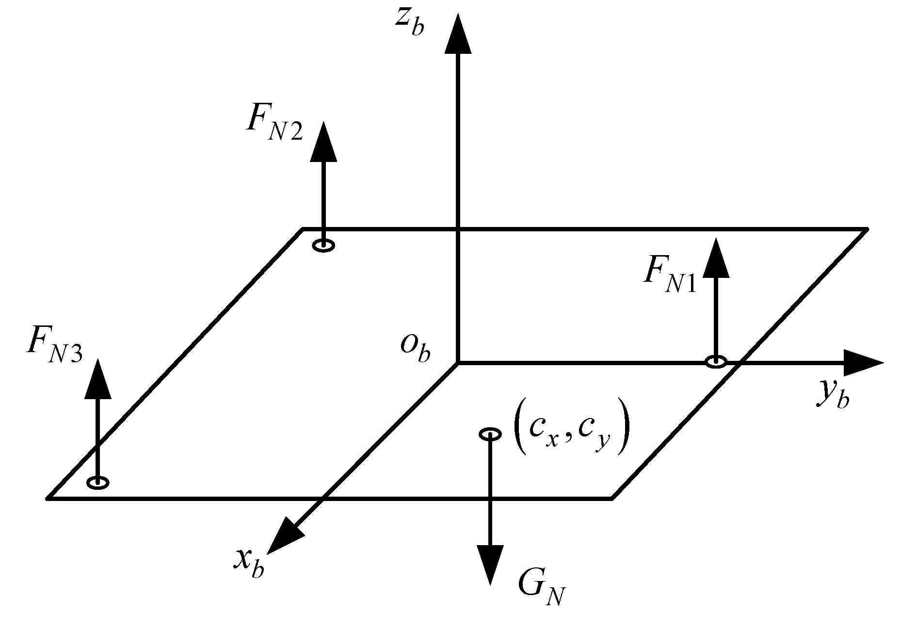
Because the simulator has an uneven mass distribution, the following multipoint support method is designed to find the centroid in the plane. As shown in Figure 11, three air bearings at the bottom of the simulator are considered to be the supporting points. Three reaction forces F N 1 , F N 2 , F N 3 are measured with three electronic balances concurrently. The centroid x c , y c can be obtained by the following moment balance equation
M o F = 0
where G N is the total mass of the simulator, which can be calculated with the following formula
G N = F N 1 + F N 2 + F N 3
The calculated centroid is shown in Table 3, and the results show that the changing scope of the centroid is small as the CO2 mass in the tank increases. The error between the real centroid and the geometric center is within an acceptable range.

4.2. Single Thruster Force and Consumption

The performance of the thrusters determines the several important indications of the simulator, which include accurate modeling in the numerical simulation, the control input, and the moment of inertia estimation. Drilled-bolt nozzles have typically been used in recent studies [21,23], but their machining accuracy has a considerable effect on thruster performance. Even with the commercial Laval nozzles used in this paper, it is still necessary to characterize all thrusters separately.
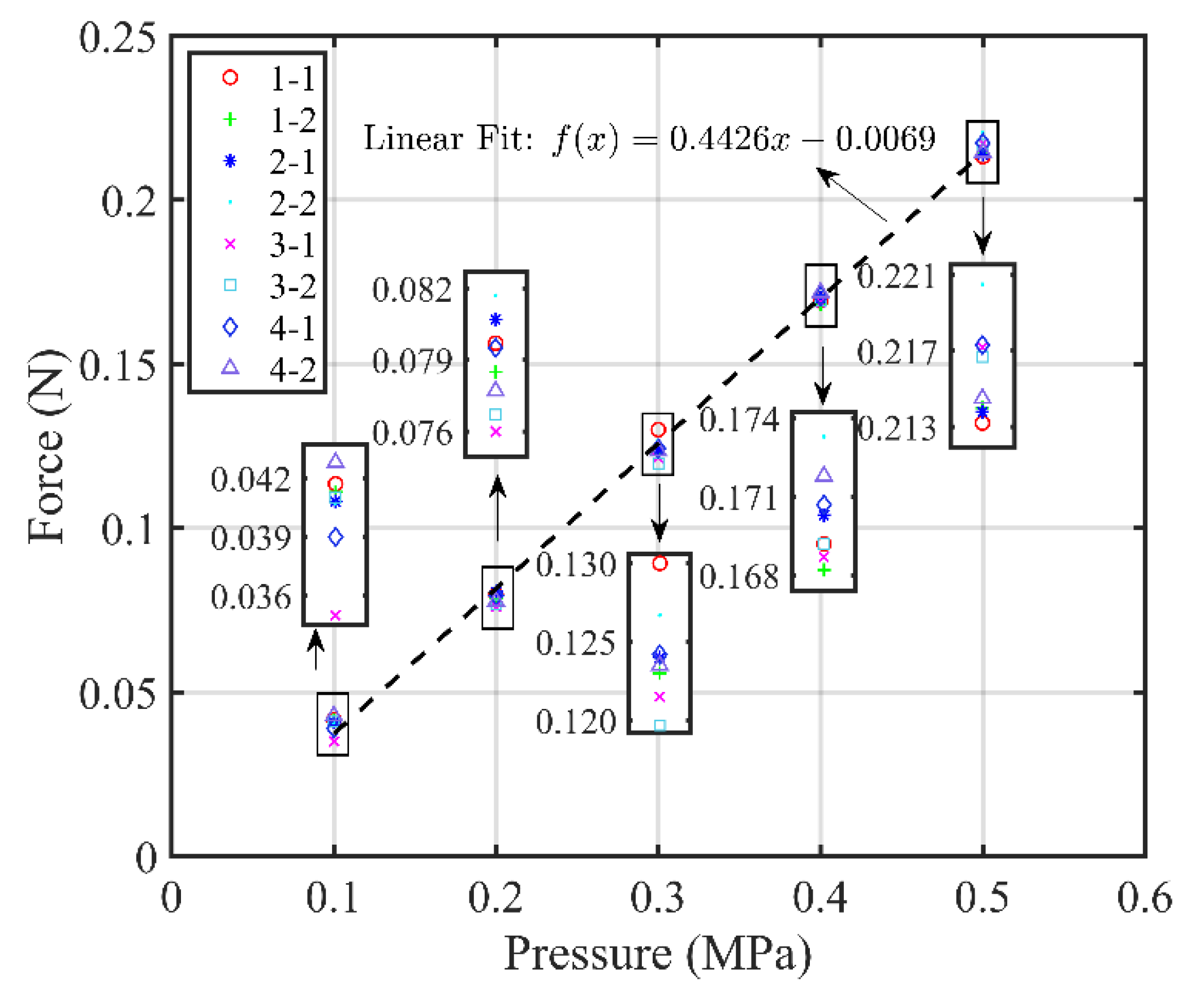
Because the thruster force is strongly affected by the pressure regulator setting, the nominal performance of a single thruster must be characterized at different CO2 pressures. Then, a load cell is used to measure the maximum force produced by the thruster. To ensure the reliability and repeatability of the results, six tests are repeated at a given operating pressure for each thruster. A resolution of 0.001 N is used to measure forces due to instabilities, even though the load cell has a higher resolution. The results are shown in Figure 12, which shows that there are small differences between each thruster at the same pressure, thereby verifying that each thruster has an equal contribution to the produced force.
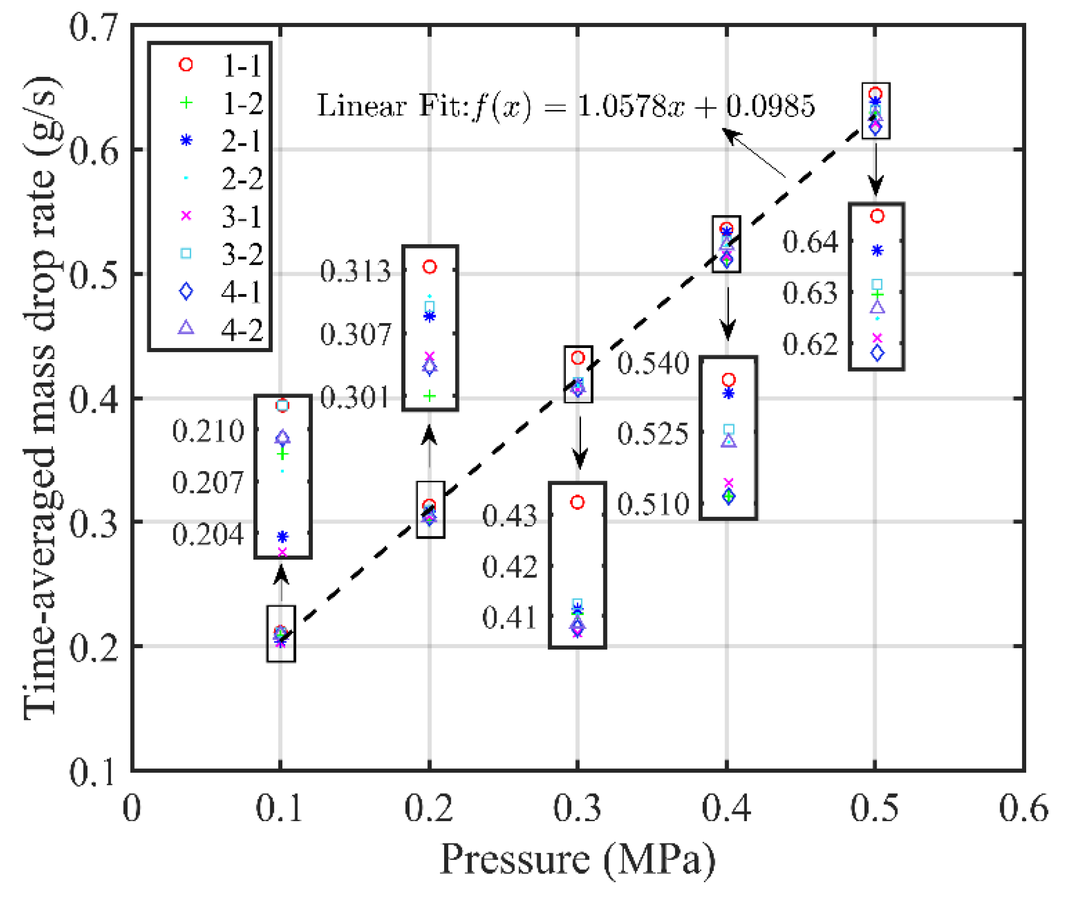
A single thruster was fired during a given time interval (5 s, 10 s, and until 30 s) to measure CO2 consumption. To diminish man-made measurement errors, each operation time interval was controlled by the ROS timer, which was also used in the later consumption experiments. Unlike compressed air, the outlet pressure of the CO2 tank was found to be relatively stable within a certain range. Thus, the single thruster consumption and the single thruster force could be measured concurrently. Consumption was then recorded using an electronic balance with a resolution of 0.1 g. Note that the supply to the air bearings was closed in the above test. CO2 consumption is shown in Figure 13. There are some small variations in the mass drop between each thruster, which could be attributed to assembly errors, manual reading errors, or ice caused by CO2 emissions.
Finally, much more concise results are provided in Table 4. The measurement biases from these tests are small. With the augmentation of the supply pressure, the measured force and consumption rate increased accordingly, and the relation was nearly linear under the experimental conditions. Thus, each thruster likely provides an equal contribution to the force produced and gas consumed.

4.3. Multiple Thrusters Force and Consumption

When the simulator is used in a simulation, two, three, or four thrusters are typically enabled concurrently. Thus, it is necessary to perform multiple thruster force and consumption tests. Similar to the previous section, the multiple thruster tests were conducted identically to the single thruster tests, with the exception that multiple thrusters are activated concurrently. Due to the eight-channel relay module, multiple thrusters could be simultaneously opened (or closed) using one line of command code, which facilitates the operation of the following experiments. For example, the operation time of multiple thrusters could be exactly controlled simultaneously.
The force measurements of the multiple thrusters were considered first. Any two, three, or four thrusters can be selected to operate within a given time. The main results are listed in Table 5, which indicate that the average thruster force is markedly less than that of the single thruster test. However, at the same supply pressure, the force loss does not monotonically increase with an increase in the number of activated thrusters. The force loss of each thruster is small and typically accounts for less than 5% of the single thruster force. This phenomenon could be due to the difference in the length of the pipeline. However, this experiment still proves that the maximum flow rate in this testbed provides a sufficient CO2 supply for every thruster.
The CO2 consumption results are also given in Table 5. By comparing these results with those from the single-thruster consumption tests, the relationship between consumption and supply pressure was nearly linear when opening multiple thrusters.
The maximum flow from the tank of the testbed can thus supply at least four thrusters adequately. The measured force loss is unavoidable when opening two or more thrusters, but is small enough and cannot increase in proportion to the number of thrusters. Therefore, this characteristic must be considered when implementing the position control loop, and the more complex control laws may benefit from such a trend.

4.4. Air Bearing Consumption

To acquire a baseline estimate of CO2 consumption while levitating over a given period, a float duration experiment was performed. For this experiment, the tank was filled with 0.8 kg CO2, which then allows only three air bearings to work concurrently. The gas consumption was recorded by an electronic balance every five minutes until the stored CO2 weighed less than 0.2 kg. Note that the gas supply to the thrusters was rejected during these tests. The air bearing consumption under different supply pressures is shown in Table 6. While the supply pressure is regulated to 0.1 MPa, the simulator cannot float above the surface of the granite. Hence, 0.1 MPa should be excluded from this test. In addition, at least 0.2 kg CO2 should be ensured in the tank for consistency, even though the simulator can still float freely below 0.2 kg. Finally, after comprehensively considering the thruster force value and the CO2 consumption of the thrusters and the air bearings, 0.3 MPa was chosen as the working pressure for the simulator in all subsequent experiments. Thus, the simulator can float above the granite surface for more than 50 min.
Additionally, the CO2 tank cools markedly when exhausting, which can result in a temperature decrease in the tank and the regulation valve. The output pressure falls due to condensation in the tank, which has a strong effect of supplying CO2 to the air bearings and the thrusters, particularly if multiple thrusters are opened concurrently. To evaluate the available operation time and the dynamic parameters of the simulator more accurately, future testbed updates should ask the user to input the initial simulator mass and indoor temperature value or could a microelectronic force sensor and temperature meter could be used instead.

4.5. Moment of Inertia

Similar to the center of mass of the simulator, the moment of inertia also plays a critical role in the system dynamics modeling. To estimate the moment of inertia I Z Z of the simulator on the granite, it was assumed that the linear and angular accelerations of the simulator due to friction while the thrusters are firing are the same as the accelerations due to friction once the thrusters have closed and the simulator is coasting [
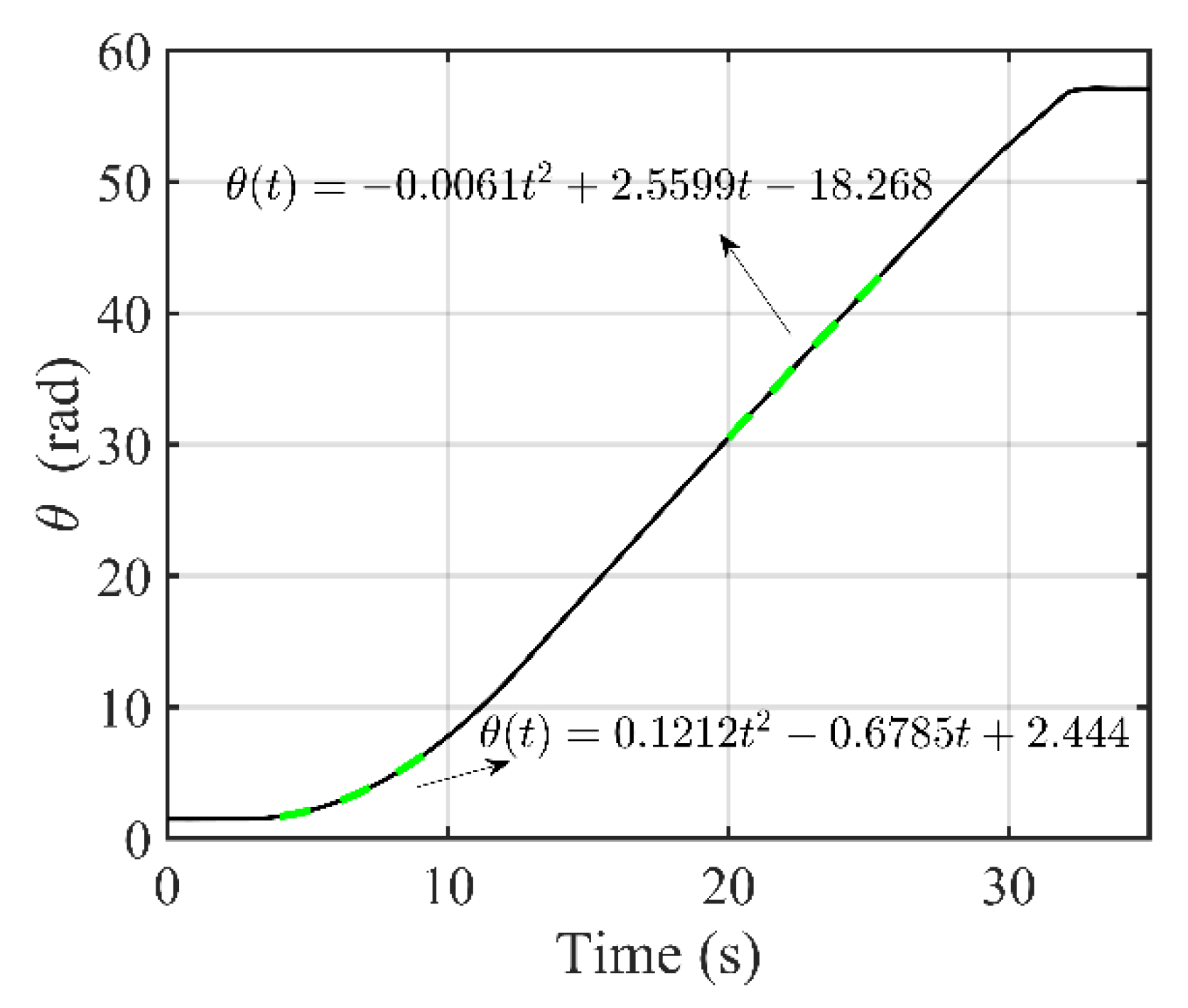
22]. The first step of the experiment is to apply a torque produced by two tangential thrusters to the stationary simulator for a given time interval, where the attitude data are recorded using the OptiTrack camera system. Next, the portions of the attitude data when the thrusters are opened are fit to the second-order model θ t = b 2 t 2 + b 1 t 1 + b 0 , and the angular accelerations are obtained by a θ t = 2 b 2 t = τ t τ f / I Z Z and a θ f = 2 b 2 f = τ f / I Z Z , where τ t is the torque produced by two thrusters applied to the simulator, τ f is the torque produced by friction while the thrusters have closed, and the firing duration of the thrusters is 10 s in all cases. A typical test is shown in Figure 14, and the pressure regulator here is set to 0.3 MPa. As shown in Figure 14, although the operation time of the two thrusters is 10 s, only the middle 6 s are used to reduce error, similarly to the deceleration process. These experiments are performed several times to obtain more reliable data, where the average I zz is 0.1445 kg·m2 and the variance is 0.0045.
Additionally, to decrease other environmental disturbances as much as possible, measures that include thorough granite surface cleaning and the same starting point at each iteration are implemented before each separate set of experiments. Aerodynamic drag is ignored in these tests because the maximum velocity of the simulator is sufficiently small.

4.6. System Latency

To quantify the system latency of the simulator, the following series of descriptions are provided. The onboard Jeston Xavier NX computer is flashed by JetPack 4.5.1 with the L4T 32.5.1 Archive, which includes Linux Kernel 4.9 and a sample filesystem based on Ubuntu 18.04. First, the prebuilt Real-Time Kernel Package for Jeston AGX Xavier was patched to the Linux kernel, and the maximum latency of the onboard operating system was bounded at 80 μs. Second, the time consumptions of the Receive node and Control node were calculated with the ROS timestamp. Finally, the on/off switching time of the relay module and the solenoid valve are given in their product manuals. All results are summarized in Table 7. Therefore, it is easy to calculate that the maximum system latency is approximately 4.05 ms with which to simultaneously open the specified thrusters, and 4.65 ms to close all thrusters. Future work should determine whether the nominal latency of the relay module and the solenoid valve is correct by using an oscilloscope to measure the timing and behavior of the real digital outputs.

5. Case Studies

To experimentally demonstrate the capabilities of the SOOST planar testbed, two typical cases were designed to move the simulator to a specified point at a pre-determined attitude angle, where the OptiTrack camera system was used in the first case for navigation, and in the second case only the onboard D435i camera was used.

5.1. Case Study Setup

The performances of the LSF estimator, the PWPF modulator, and the modified DCF-based visual method are described as follows. Table 8 shows the related test parameters, which can be further divided into the following three categories: the LSF estimator, the PWPF modulator, and the marker parameters. The following are the results when choosing the related parameters of the LSF velocity estimator, the PWPF modulator, and the proposed visual method presented in the remainder of this section. Case study results are provided in the next section.

5.1.1. Performance of the LSF Estimator

A set of motion raw data of the simulator from the OptiTrack camera system was used to estimate the velocity using different methods. The sampling frequency of the OptiTrack camera system was set to 30 Hz. The velocity of the simulator increased due to the thruster firing at the beginning of the experiment, and then, the velocity was adjusted by the thrusters to observe the capacity of the velocity estimator to manage emergencies.
Considering the motion in the x-direction as an example, the corresponding velocities of the simulator were determined by using the first-order backward difference (FBD) method and LSF estimator. The LSF estimator shown in Figure 15a,b uses 20 points for fitting, namely, M = 20, but the interpolation polynomials are of the 1st and 2nd orders, respectively.
As shown in Figure 15, the FBD velocity estimator can generate larger data jitter, which includes obvious high-frequency components. However, the LSF estimator demonstrates a thorough competence when managing these issues, and the curve obtained by the first-order LSF estimator shown in Figure 15a is particularly smooth. The thrusters first opened at approximately 2 s and closed at approximately 12 s. Then, they opened again at approximately 16 s and closed at 17 s. Considering the velocity variations shown in the following figure, the LSF estimator achieves a similar transient response performance to the FBD estimator, and the second-order LSF estimator exhibits no marked time delay, while the first-order estimator lags marginally.

5.1.2. Performance of the PWPF Modulator

The parameters of the PWPF modulator are reported in Table 8 according to the literature [45], where Um is the maximum value of force (produced by a single normal thruster) or torque (produced by two opposite tangential thrusters).
Figure 16 shows the modulation results of the control input signal f(t) = 0.02 cos (t), f(t) = 0.12 cos (t), and f(t) = 0.4 cos (t). Figure 16c shows that if the maximum expected input signal markedly exceeds the maximum output Um of the ST, then the impulse provided by the modulated pulse signal will be less than the expected impulse, and the pulse sequence obtained at this time is similar to the control signal limited by input saturation. Thus, the input saturation is automatically included by the PWPF modulator and will no longer be considered in a later section.

5.1.3. Performance of the Visual Navigation Method

The performance of the designed visual method is described from the following two perspectives: position estimation performance and attitude estimation performance.
First, the position estimation precision can be obtained by comparing the real and measured distances between o 1 m and o 2 m at the marker array. As shown in Figure 10, the distance d m between o 1 m and o 2 m can be obtained by
d m = 2 d gap + d size
According to Table 8, the real d m is 0.05 m, and the results are shown in Figure 17. The experimental test was performed over a period of 40 s, and the camera was in constant motion for the first 30 s but remained still for the remainder of the test. Figure 17 shows that the maximum error between the real and measured values is approximately 0.8 mm during the first 30 s, and is smaller than 0.2 mm when the camera is at rest. These results likely occur because camera motion has an impact on corner recognition, but the position estimation error is still within an acceptable range.
Second, a contrasting experiment was designed to illustrate the attitude estimation performance for the modified DCF-based method. The relevant equipment is shown in Figure 18. While the simulator is in motion, the impulse and vibration caused by the thruster force leads the onboard camera to fluctuate marginally back and forth. Thus, the simulator was controlled to swing back and forth by the experimenter at a given amplitude. The marker array and the original marker (ID = 5) could be measured simultaneously. To ensure the reliability and accuracy of the experimental results, the two markers were designed to be the same size; the sizes of the two red boxes in Figure 18 are the same. The projections for the two markers are all near the image center to mitigate image distortions. Figure 19 depicts the experimental results for a period of 4 s. Evident oscillation and abrupt changes were found in the peak amplitude of the green curve (the results for the single original marker) due to a low precision for corner estimation caused by image blur during relative motion. Compared with the former, the black curve is smooth and steady in the same environment.

5.2. Case Study Results

The PD controllers for the two experiments can be formulated as
f x = k 1 X X d k 2 X ˙ f y = k 1 Y Y d k 2 Y ˙ τ = k 3 θ θ d k 4 θ ˙
where [ X d , Y d , θ d ] T is the desired value, and k 1 , k 2 , k 3 , k 4 are the controller parameters, which are listed in Table 9.

5.2.1. Case I

The experimental results using the external visual system are shown in Figure 20, and the experimental test was performed for 60 s. Figure 20a–c shows the absolute coordinates and attitude of the simulator. The position and attitude of the simulator fluctuate marginally back and forth near the target value, due to the limited precision of the PWPF modulator of the thrust and excessive minimum impulse torque. Therefore, the range of the coordinate fluctuation of the simulator is small, yielding average steady-state errors of approximately 1.5 mm, 0.5 mm, and 0.0 deg, respectively. Additionally, the velocities and the angular velocity of the simulator throughout the experimental test are shown in Figure 20d–f. Similar to the first three graphs, the velocities fluctuate marginally at a steady-state due to the binary nature of the thruster force.

5.2.2. Case II

To demonstrate the visual navigation method proposed in this paper, only the designed marker array was used to complete the experiment. The experimental test was performed over a period of 20 s, and the results shown in Figure 21 were obtained using the onboard camera. Similar to Case I, the position and attitude of the simulator fluctuate back and forth near the target value. However, the oscillation amplitudes are greater than for the former results, which may be due to the coupling between the onboard visual measurement and control system, or the image blur during relative motion. However, the stable periodic motion of the simulator near the target value shows that the proposed method still has a certain level of reliability, which helps to provide a low-cost auxiliary navigation method to use when it does not have a high-precision external visual system.

6. Conclusions

This paper described the design of the SOOST situated in the SKLMCMS at NUAA, which primarily includes a detailed description of the spacecraft simulator. The simulator can operate on the testbed under the motion of two translational and one rotational DOF with quasi-frictionless and microgravity dynamic behavior, and the eight onboard thrusters could provide control forces or torques to maneuver the simulator on the granite testbed. The thrusters are equivalent to the actuators found in real orbital spacecraft and enhance the relevant dynamic equivalence.
The key parameters of the SOOST are identified by a series of systematic characterization tests, which are required in order to build an accurate model for attitude and position control. The centroid of the redesigned testbed system is determined to be within 6 mm of the geometric center, and the moment of inertia on the granite is calculated to be 0.1445 kg·m2. The consumption of the thrusters and the air bearings were discussed in detail for different supply pressures. For example, with a supply pressure of 0.3 MPa, any four thrusters require a consumption rate of 1.656 g/s; all three air bearings require a consumption rate of 0.187 g/s; and a single thruster’s force is 0.12 N. Then, the maximum system latency was found to be approximately 4.05 ms to simultaneously enable the thrusters, and 4.65 ms to close all thrusters. In addition, a modified DCF-based method was presented to provide autonomous navigation without an external visual system. The results of various experiments demonstrate the efficiency and performance of the proposed method.
With a series of systematic characterization tests, a fundamental testbed study could provide high repeatability, consistency, and human-error reduction. Thus, the SOOST developed by NUAA can serve as a valuable tool with which to develop control methods for simulating spacecraft dynamics and control.

Author Contributions

Z.H. and W.Z. completed preliminary research; Z.H. conceived and wrote the paper; T.C., H.W. and D.J. supervised the overall work and reviewed it. All authors have read and agreed to the published version of the manuscript.

Funding

This work was supported by the National Natural Science Foundation of China under Grant 11832005, Grant 11732006 and the Postgraduate Research & Practice Innovation Program of Jiangsu Province under Grant KYCX21_0182.

Institutional Review Board Statement

Not applicable.

Informed Consent Statement

Not applicable.

Data Availability Statement

Not applicable.

Conflicts of Interest

The authors declare no conflict of interest.

References

  1. Modenini, D.; Bahu, A.; Curzi, G.; Togni, A. A dynamic testbed for nanosatellites attitude verification. Aerospace 2020, 7, 31. [Google Scholar] [CrossRef] [Green Version]
  2. Cheng, A.F.; Atchison, J.; Kantsiper, B.; Rivkina, A.S.; Sticklea, A.; Reeda, C.; Galvezb, A.; Carnellib, I.; Michelc, P.; Ulamecd, S. Asteroid impact and deflection assessment mission. Acta Astronaut. 2015, 115, 262–269. [Google Scholar] [CrossRef] [Green Version]
  3. Perez, F.; Modenini, D.; Vazquez, A.; Aguado, F.; Tubío, R.; Dolgos, G.; Tortora, P.; Gonzalez, A.; Manghi, R.L.; Zannoni, M.; et al. DustCube, a nanosatellite mission to binary asteroid 65803 Didymos as part of the ESA AIM mission. Adv. Space Res. 2018, 62, 3335–3356. [Google Scholar] [CrossRef]
  4. Michel, P.; Kueppers, M.; Sierks, H.; Carnelli, I.; Cheng, A.F.; Mellab, K.; Granvik, M.; Kestila, A.; Kohout, T.; Muinonen, K.; et al. European component of the AIDA mission to a binary asteroid: Characterization and interpretation of the impact of the DART mission. Adv. Space Res. 2018, 62, 2261–2272. [Google Scholar] [CrossRef] [Green Version]
  5. Michel, P.; Cheng, A.; Küppers, M.; Pravec, P.; Blume, J.; Delbo, M.; Green, S.F.; Rosenblatt, P.; Tsiganish, K.; Vincent, J.B.; et al. Science case for the Asteroid Impact Mission (AIM): A component of the Asteroid Impact & Deflection Assessment (AIDA) mission. Adv. Space Res. 2016, 57, 2529–2547. [Google Scholar]
  6. Quadrelli, M.B.; Wood, L.J.; Riedel, J.E.; McHenry, M.C.; Aung, M.; Cangahuala, L.A.; Volpe, R.A.; Beauchamp, P.M.; Cutts, J.A. Guidance, navigation, and control technology assessment for future planetary science missions. J. Guid. Control Dyn. 2015, 38, 1165–1186. [Google Scholar] [CrossRef] [Green Version]
  7. Wen, H.; Jin, D.P.; Hu, H. Ground-based experimental study on deployment and retrieval control of tethered satellite. J. Vib. Eng. Technol. 2010, 23, 7–11. [Google Scholar]
  8. Wen, H. Dynamic Control for Deployment and Retrieval of Tethered Satellite Systems. Ph.D. Thesis, Nanjing University of Aeronautics and Astronautics, Nanjing, China, 2009. [Google Scholar]
  9. Chen, H.; Wen, H.; Jin, D.; Hu, H. Experimental studies on tethered satellite systems. Adv. Appl. Mech. 2013, 43, 174–184. [Google Scholar]
  10. Chen, T. State Consensus and Autonomous Assembly for a Team of Flexible Spacecraft. Ph.D. Thesis, Nanjing University of Aeronautics and Astronautics, Nanjing, China, 2017. [Google Scholar]
  11. Yang, S.; Wen, H.; Hu, Y.; Jin, D. Coordinated motion control of a dual-arm space robot for assembling modular parts. Acta Astronaut. 2020, 177, 627–638. [Google Scholar] [CrossRef]
  12. Chen, Y.; Wen, H.; Jin, D. Design and experiment of a noncontact electromagnetic vibration isolator with controllable stiffness. Acta Astronaut. 2020, 168, 130–137. [Google Scholar] [CrossRef]
  13. Wei, Z.; Wen, H.; Hu, H.; Jin, D. Ground experiment on rendezvous and docking with a spinning target using multistage control strategy. Aerosp. Sci. Technol. 2020, 104, 105967. [Google Scholar] [CrossRef]
  14. Yu, B.S.; Huang, Z.; Geng, L.L.; Jin, D.P. Stability and ground experiments of a spinning triangular tethered satellite formation on a low earth orbit. Aerosp. Sci. Technol. 2019, 92, 595–604. [Google Scholar] [CrossRef]
  15. Huang, Z.; Lu, Y.; Wen, H.; Jin, D. Ground-based experiment of capturing space debris based on artificial potential field. Acta Astronaut. 2018, 152, 235–241. [Google Scholar] [CrossRef]
  16. Yu, B.S.; Geng, L.; Wen, H.; Jin, D.P. Ground-based experiments of tether deployment subject to an analytical control law. Acta Astronaut. 2018, 151, 253–259. [Google Scholar] [CrossRef]
  17. Zappulla, R.; Virgili-Llop, J.; Zagaris, C.; Park, H.; Romano, M. Dynamic air-bearing hardware-in-the-loop testbed to experimentally evaluate autonomous spacecraft proximity maneuvers. J. Spacecr. Rockets 2017, 54, 825–839. [Google Scholar] [CrossRef] [Green Version]
  18. Virgili-Llop, J.; Drew, J.V.; Zappulla, R.; Romano, M. Laboratory experiments of resident space object capture by a spacecraft-manipulator system. Aerosp. Sci. Technol. 2017, 71, 530–545. [Google Scholar] [CrossRef]
  19. Sabatini, M.; Palmerini, G.B.; Gasbarri, P. Synergetic approach in attitude control of very flexible satellites by means of thrusters and PZT devices. Aerosp. Sci. Technol. 2020, 96, 105541. [Google Scholar] [CrossRef]
  20. Sabatini, M.; Palmerini, G.B.; Ribet, M.; Gasbarri, P. Effects of a High Fidelity Filter on the attitude stabilization of a flexible spacecraft. Acta Astronaut. 2018, 151, 260–269. [Google Scholar] [CrossRef]
  21. Wapman, J.D.; Sternberg, D.C.; Lo, K.; Wang, M.; Jones-Wilson, L.; Mohan, S. Jet Propulsion Laboratory small satellite dynamics testbed planar air-bearing propulsion system characterization. J. Spacecr. Rockets 2021, 58, 1–18. [Google Scholar] [CrossRef]
  22. Sternberg, D.C.; Pong, C.; Filipe, N.; Mohan, S.; Johnson, S.; Jones-Wilson, L. Jet Propulsion Laboratory small satellite dynamics testbed simulation: On-orbit performance model validation. J. Spacecr. Rockets. 2018, 55, 322–334. [Google Scholar] [CrossRef]
  23. Nieto-Peroy, C.; Palmerini, G.; de Oliveira, É.J.; Gasbarri, P. Simulation of spacecraft formation maneuvers by means of floating platforms. In Proceedings of the IEEE Aerospace Conference, Big Sky, MT, USA, 6–13 March 2021. [Google Scholar]
  24. Kwok-Choon, S.; Buchala, K.; Blackwell, B.; Lopresti, S.; Wilde, M.; Go, T. Design, fabrication, and preliminary testing of air-bearing test vehicles for the study of autonomous satellite maneuvers. In Proceedings of the 31st Florida Conference on Recent Advances in Robotics, Orlando, FL, USA, 10–11 May 2018. [Google Scholar]
  25. Virgili-Llop, J.; Zagaris, C.; Zappulla, R.; Bradstreet, A.; Romano, M. A convex-programming-based guidance algorithm to capture a tumbling object on orbit using a spacecraft equipped with a robotic manipulator. Int. J. Rob. Res. 2019, 38, 40–72. [Google Scholar] [CrossRef]
  26. Virgili-Llop, J.; Romano, M. Simultaneous capture and detumble of a resident space object by a free-flying spacecraft-manipulator system. Front. Robot. AI 2019, 6, 14. [Google Scholar] [CrossRef] [Green Version]
  27. Laurenzi, S.; Rufo, D.; Sabatini, M.; Gasbarri, P.; Palmerini, G.B. Characterization of deployable ultrathin composite boom for microsatellites excited by attitude maneuvers. Compos. Struct. 2019, 220, 502–509. [Google Scholar] [CrossRef]
  28. Sabatini, M.; Palmerini, G.B.; Monti, R.; Gasbarri, P. Image based control of the "PINOCCHIO" experimental free flying platform. Acta Astronaut. 2014, 94, 480–492. [Google Scholar] [CrossRef]
  29. Mantellato, R.; Lorenzini, E.C.; Sternberg, D.; Gasbarri, P. Simulation of a tethered microgravity robot pair and validation on a planar air bearing. Acta Astronaut. 2017, 138, 579–589. [Google Scholar] [CrossRef]
  30. Sternberg, D.C. Development of an Incremental and Iterative Risk Reduction Facility for Robotic Servicing and Assembly Missions; Massachusetts Institute of Technology Department of Aeronautics and Astronautics: Cambridge, MA, USA, 2014. [Google Scholar]
  31. Ivanov, D.; Koptev, M.; Ovchinnikov, M.; Tkachev, S.; Proshunin, N.; Shachkov, M. Flexible microsatellite mock-up docking with non-cooperative target on planar air bearing test bed. Acta Astronaut. 2018, 153, 357–366. [Google Scholar] [CrossRef]
  32. Bevilacqua, R.; Hall, J.S.; Horning, J.; Romano, M. Ad hoc wireless networking and shared computation for autonomous multirobot systems. J. Aeros. Comp. Inf. Com. 2009, 6, 328–353. [Google Scholar] [CrossRef] [Green Version]
  33. Rybus, T.; Seweryn, K. Planar air-bearing microgravity simulators: Review of applications, existing solutions and design parameters. Acta Astronaut. 2016, 120, 239–259. [Google Scholar] [CrossRef]
  34. Du, X.; Liu, B.; Fang, Z.; Jun-an, Z. Research on Laval nozzle and overall simulation analysis based on high speed precision air bearing spindle pneumatic turbine system. In Proceedings of the International Conference on Precision Machining, Non-Traditional Machining and Intelligent Manufacturing, Xi’an, China, 22–24 November 2019. [Google Scholar]
  35. He, X.; Feng, X.; Zhong, M.; Gou, F.; Deng, S. The influence of Laval nozzle throat size on supersonic molecular beam injection. J. Mod. Transp. 2014, 22, 118–121. [Google Scholar] [CrossRef] [Green Version]
  36. Reghenzani, F.; Massari, G.; Fornaciari, W. The real-time Linux kernel: A survey on PREEMPT_RT. ACM Comput. Surv. 2019, 52, 1–36. [Google Scholar] [CrossRef]
  37. Gupta, S.; Durak, U. RESTful software architecture for ROS-based onboard mission system for drones. In Proceedings of the AIAA SciTech Forum, Orlando, FL, USA, 6–10 January 2020. [Google Scholar]
  38. Koopman, P.; Chakravarty, T. Cyclic Redundancy Code (CRC) polynomial selection for embedded networks. In Proceedings of the International Conference on Dependable Systems and Networks, Florence, Italy, 28 June–1 July 2004. [Google Scholar]
  39. Brown, R.H.; Schneider, S.C.; Mulligan, M.G. Analysis of algorithms for velocity estimation from discrete position versus time data. IEEE Trans. Ind. Electron. 1992, 39, 11–19. [Google Scholar] [CrossRef]
  40. Song, G.; Agrawal, B.N. Vibration suppression of flexible spacecraft during attitude control. Acta Astronaut. 2001, 49, 73–83. [Google Scholar] [CrossRef] [Green Version]
  41. Guglieri, G.; Maroglio, F.; Pellegrino, P.; Torre, L. Design and development of guidance navigation and control algorithms for spacecraft rendezvous and docking experimentation. Acta Astronaut. 2014, 94, 395–408. [Google Scholar] [CrossRef]
  42. Romero-Ramirez, F.J.; Muñoz-Salinas, R.; Medina-Carnicer, R. Tracking fiducial markers with discriminative correlation filters. Image Vis. Comput. 2021, 107, 104094. [Google Scholar] [CrossRef]
  43. Bradski, G.; Kaehler, A. Learning OpenCV: Computer Vision in C++ with the OpenCV Library, 2nd ed.; O’Reilly Media, Inc.: Sebastopol, CA, USA, 2013. [Google Scholar]
  44. Lepetit, V.; Moreno-Noguer, F.; Fua, P. EPnP: Accurate non-iterative O(n) solution to the PnP problem. Int. J. Comput. Vis. 2009, 81, 155. [Google Scholar] [CrossRef] [Green Version]
  45. Hu, Q.; Ma, G. Variable structure control and active vibration suppression of flexible spacecraft during attitude maneuver. Aerosp. Sci. Technol. 2005, 94, 307–317. [Google Scholar] [CrossRef]
Figure 1. Overview of the primary elements of the SOOST system.
Aerospace 09 00246 g001
Figure 2. Hardware layout of the fourth-generation simulator.
Aerospace 09 00246 g002
Figure 3. Mechanical structure layout of the spacecraft simulator.
Aerospace 09 00246 g003
Figure 4. Electrical supply and signal block diagram of the testbed.
Aerospace 09 00246 g004
Figure 5. Schematic view of the pneumatic subsystem.
Aerospace 09 00246 g005
Figure 6. Typical thruster structure.
Aerospace 09 00246 g006
Figure 7. Thruster numbering and coordinate system definitions.
Aerospace 09 00246 g007
Figure 8. Overview of the system software architecture.
Aerospace 09 00246 g008
Figure 9. PWPF modulator.
Aerospace 09 00246 g009
Figure 10. A new marker array.
Aerospace 09 00246 g010
Figure 11. Schematic view of the multipoint supporting method.
Aerospace 09 00246 g011
Figure 12. Single thruster force characterization data with the first-order fit.
Aerospace 09 00246 g012
Figure 13. Single thruster consumption characterization data with the first-order fit.
Aerospace 09 00246 g013
Figure 14. Estimate for the moment of inertia with a second-order fit.
Aerospace 09 00246 g014
Figure 15. Velocity estimate using the LSF and FBD estimators. (a) N = 1, (b) N = 2.
Aerospace 09 00246 g015
Figure 16. Results of the PWPF modulator in a cosine function with different amplitudes. (a) f(t) = 0.02 cos (t), (b) f(t) = 0.12 cos (t), (c) f(t) = 0.4cost(t).
Aerospace 09 00246 g016aAerospace 09 00246 g016b
Figure 17. The measurements for the distance d m .
Aerospace 09 00246 g017
Figure 18. Contrasting experiment for attitude measurement.
Aerospace 09 00246 g018
Figure 19. Attitude measurement results.
Aerospace 09 00246 g019
Figure 20. Position and velocity of the simulator during the entire maneuver using the external visual system. (a) Position in the x-direction, (b) Position in the y-direction, (c) Attitude about the z-axis, (d) Velocity in the x-direction, (e) Velocity in the y-direction, (f) Angular velocity about the z-axis.
Aerospace 09 00246 g020aAerospace 09 00246 g020b
Figure 21. Position and velocity of the simulator during the entire maneuver using the onboard camera. (a) Position in the x-direction, (b) Position in the y-direction, (c) Attitude about the z-axis, (d) Velocity in the x-direction, (e) Velocity in the y-direction, (f) Angular velocity about the z-axis.
Aerospace 09 00246 g021
Table 1. Electrical properties of the primary electrical components.
ComponentInput Voltage (Volt)Power Consumption (Watt)
Jeston Computer1910
Display5 (USB)2.5
D435i camera5 (USB)4.5
Relay module240.6
Serial converter 5 (USB)1.5
ZigBee module5 (USB)0.7
Solenoid valve247
Table 2. Pneumatic properties of the testbed.
ParameterValue
Maximum portable CO2 mass 0.8 kg
Tank volume1.1 L
Operating pressure of solenoid valve0.05~0.6 MPa
Maximum allowable pressure of air bearing0.689 MPa
Nominal size of Laval nozzle0.7 mm
Air-bearing pressure (regulated)0.3 MPa
Thruster pressure (regulated)0.3 MPa
Table 3. Total mass and centroid data.
Total Mass (g)Centroid’s Coordinates (mm)
9642.2 (with no load tank)(5.6, −4.6)
10,442.2 (with full load tank)(5.7, −3.3)
Table 4. Single thruster force and consumption data.
Pressure
(MPa)
Averaged Force
(N)
Force ErrorTime-Averaged Consumption (g/s)Consumption Error
0.10.0400.0020.20810.003
0.20.0790.0020.3069 0.004
0.30.124 0.0030.41250.008
0.40.170 0.0020.52230.009
0.50.216 0.0030.62930.009
Table 5. Multiple thruster force and consumption data.
ThrusterPressure
(MPa)
Averaged Force
(N)
Averaged
Force Loss (N)
Time-Averaged
Consumption (g/s)
Any two0.10.0380.0020.432
0.20.0740.0050.622
0.30.1190.0050.820
0.40.1650.0051.028
0.50.2110.0051.220
Any three0.10.0380.0020.634
0.20.0740.0050.910
0.30.1210.0031.274
0.40.1670.0031.596
0.50.2130.0031.878
Any four0.10.0380.0020.848
0.20.0760.0031.240
0.30.1200.0041.656
0.40.1640.0062.084
0.50.2100.0062.496
Table 6. Air bearing consumption data.
Pressure (MPa)Time-Averaged Consumption (g/s)
0.20.106
0.30.187
0.40.288
0.50.387
Table 7. System latency characteristics.
Minimum
Latency (ms)
Average
Latency (ms)
Maximum
Latency (ms)
Nominal
Latency (ms)
Operating latency0.0030.0100.049/
Receive node0.0140.0490.078/
Control node0.0370.2380.136/
Relay module ON///3.0
Relay module OFF///4.0
Solenoid valve ON///0.8
Solenoid valve OFF///0.4
Table 8. Test parameters.
LSF
Parameters
ValuesPWPF
Parameters
ValuesMarker Array
Parameters
Values
M20Km20dgap0.005 m
N2Tm0.5dsize0.04 m
//Um0.12 N or 0.036 Nm//
//Eon0.75 × Um//
//Eoff0.25 × Um//
Table 9. Controller parameters.
Parameters Case ICase II
[ X d , Y d , θ d ] T [ 0.6   m , 0.8   m , 45 ] T [ 0.0   m , 0.4   m , 0.0 ] T
k 1 8.55.0
k 2 30.030.0
k 3 2.01.5
k 4 15.015.0
Publisher’s Note: MDPI stays neutral with regard to jurisdictional claims in published maps and institutional affiliations.

