Article

Micro Coaxial Drone: Flight Dynamics, Simulation and Ground Testing

by
Victor H. Dominguez
,
Octavio Garcia-Salazar
*,†,
Luis Amezquita-Brooks
,
Luis A. Reyes-Osorio
,
Carlos Santana-Delgado
and
Erik G. Rojo-Rodriguez
Aerospace Engineering Research and Innovation Center, Faculty of Mechanical and Electrical Engineering, Autonomous University of Nuevo Leon, San Nicolas de los Garza 66455, Nuevo Leon, Mexico
*
Author to whom correspondence should be addressed.
These authors contributed equally to this work.
Aerospace 2022, 9(5), 245; https://doi.org/10.3390/aerospace9050245
Submission received: 9 February 2022 / Revised: 23 March 2022 / Accepted: 8 April 2022 / Published: 1 May 2022
(This article belongs to the Section Aeronautics)

Abstract

:
This paper describes the conceptual design of a micro coaxial unmanned aerial vehicle (MCR UAV v3.0) based on its flight dynamics and a simple aerodynamic analysis using computational fluid dynamics (CFD). In addition, a simple linear control is proposed with the pole assignment technique. The methodology proposed in this paper involves a standardized path for designing the novel micro coaxial UAV. This begins by selecting the avionics to create a primary dimensional design for a later transient and stationary CFD analysis. In effect, the mathematical model is obtained using the Newton–Euler formulation and is linearized to obtain the dynamical requirements of the vehicle. The requirements allow us to design the control scheme with a linear control technique. This process is iterative and uses a combination of flight dynamics and CFD. The control technique is based on pole assignment, ensuring a specific phase condition is used in the controller gain for the stabilization of the proposed aerial vehicle. The control scheme is analyzed once the CFD analysis is correctly performed; in this sense, the methodology proposed in this paper is capable of converging as a result of the dimensional design. This design ensures a suitable vehicle performance according to the dynamical requirements. Thus, the micro coaxial UAV is completely designed based on its flight dynamics along with a CFD analysis, generating a robust methodology.

1. Introduction

One of the most investigated fields in aeronautical engineering in the last decade was unmanned aerial vehicles (UAVs). Nowadays, specific research tends to be aimed at guidance, navigation, control of UAVs, swarms and nonconventional configurations of UAVs. All these fields have been growing constantly due to their incredible potential in military and civil applications such as recognition, control of disasters, inspection, observation, precision agriculture, vigilance and emergency aid, which require UAVs that are capable of adapting to the mission environment.
Commonly, aerial vehicles with a coaxial configuration require complex mechanisms such as tilt rotors, swashplates and stabilizer bars to control the direction of the rotor thrust vector. These mechanisms give promising results for these types of configurations, even though these are complex systems to control. Theoretical and practical contributions on UAVs with coaxial configurations have been reported in the literature, including the improvement of a new mechanism to control the vehicle motion. A swashplateless coaxial helicopter design to perform trajectory tracking and heading control maneuvers was presented in [1], and experimental results were carried out in closed-loop system using a motion capture environment. In [2], the authors presented the design, modeling and control of a single-rotor UAV, where the mathematical model, along with a control system based on cascaded P-PI and PID controllers, was simulated to demonstrate the tracking performance. Authors in [3] proposed a nonlinear control design for the trajectory tracking of a coaxial rotor UAV using exact feedback linearization and a PI observer. In that paper, simulations were carried out to demonstrate the feasibility of the proposed control strategy. In [4], the authors proposed a similar configuration of a coaxial rotor UAV for indoor missions using a spherical frame. The coaxial UAV was tested using PD and robust controllers for the lateral, longitudinal and vertical dynamics. Ref. [5] presented two different real-time control systems for a single RC coaxial helicopter. These proposed controllers were designed as LQR and H to track the desired points or paths and were presented in a numerical simulation. The authors in [6] presented a nonlinear controller based on the backstepping approach for a gun-launched micro aerial vehicle with a coaxial configuration. The controller was designed to perform trajectory tracking, and numerical and experimental results were provided.
In [7], a hierarchical controller based on a disturbance observer with finite-time convergence was proposed to solve the path tracking of a small coaxial rotor UAV. The proposed observer was designed to estimate the uncertainties and disturbances in finite time. Simulation results were carried out to show the performance of the proposed controller. In [8], a trajectory tracking problem was solved for a small coaxial-rotor UAV, by considering an adaptive fault-tolerant control with partial loss of actuator effectiveness. The results of the simulation were presented to validate the effectiveness of the proposed controller. Ref. [9], proposed a mixed algorithm based on an adaptive control, with a robust decoupling control and adaptive augmentation which were validated in a numerical simulation. These simulation results showed effective responses even under uncertainties and external disturbances. In [10], the authors presented a controller based on switching control theory for an unmanned ducted-fan helicopter. The stability analysis was performed using Lyapunov theory, and nonlinear simulations were run to demonstrate the flexibility and efficiency of the proposed algorithm. A robust controller to track orientation and position with uncertainties rejection was proposed in [11]. The controller used a backstepping-free trajectory tracking strategy for the UAV, and the Lyapunov analysis was presented. Simulation studies were shown to validate the proposed strategy. In [12], the nonlinear modeling of a gun-launched micro aerial vehicle with coaxial contra-rotating rotors was described for the hover flight mode, and the aerodynamic parameters were estimated using the Kalman filter technique. In [13], the design and analysis of a novel tail-sitter mini UAV were proposed, and free software was used in the design process. This process considered the design, aerodynamic analysis and evaluation of control modes.

1.1. State of the Art

The configuration of coaxial rotors has gained significant interest in aeronautics research in the UAV field, since the main advantage of this configuration is to generate a higher thrust than a single rotor on a small disk area. In effect, coaxial rotors are required to be aerodynamically characterized; then, thrust and torque coefficients are obtained as functions of various parameters. For instance, the authors in [14] executed a CFD simulation to obtain the aerodynamic effects of single and coaxial propellers for many pitch angles on a multicopter vehicle. The CFD results showed the interference effect, in which the lower propeller affects the upper propeller through a distorted flow orientation from upstream, especially at low pitches. In [15], the authors presented an analysis based on a CFD simulation and hovering experimental tests to obtain the performance and design parameters involving thrust, torque, power consumption, rotor spacing, rotational speed and angle of attack for a coaxial rotor aircraft. In [16], the authors presented numerical simulations and experimental tests for a hex-rotor micro UAV with coaxial rotors and different rotor spacings. The results showed the performance of the vehicle based on pressure, velocity distribution, thrust and power. The pressure and velocity were obtained using CFD, whereas the thrust and power were obtained from the experimental platform.
In [17], the authors described the solution to 3D unsteady Euler equations numerically, to simulate unsteady flows around a helicopter with a coaxial configuration. The aerodynamic interaction and the influence of the two rotors in a coaxial configuration were analyzed, and results were obtained from the CFD simulations showing that the proposed method of unstructured dynamic overset grids was efficient and robust for simulating unsteady flows around a helicopter with coaxial rotors. In [18], aerodynamic characterization was performed using a wind tunnel, for a coaxial rotor with 4 m diameter composite blades. In addition, the authors simulated a rigid coaxial rotor, employing the CFD technique to obtain the aerodynamic parameters for hover flight with fixed coaxial blades. Then, the forward condition was evaluated by changing the incidence angle of the upper rotor. Another study on the coaxial configuration was presented in [19], including experimental and computational studies of the hovering performance of micro coaxial shrouded rotors, involving factors such as blade pitch angle, rotor spacing and tip clearance. Numerical simulation of the flow field around rotor was performed using the sliding mesh method and multiple reference frame techniques, using Ansys Fluent, and the experimental tests were carried out using an ATI transducer system to obtain the force and moments measurements. Ref. [20] presented an experimental validation for a quadrotor of eight motors arranged in four coaxial pairs. Experiments with different motors and sizes of propellers were carried out to estimate the efficiency of coaxial rotors regarding the useful thrust generated by each configuration. In [21], the authors proposed a procedure that consisted of modeling the flight dynamics, with model-based parameter identification, for coaxial UAVs. This procedure included rotor dynamics and swashplate dynamics. The ground testing procedure was used to characterize the coaxial rotor, obtaining the coefficients of the thrust and angular velocities.

1.2. Problem Statement

UAVs research, development and usage have been increasing in recent years due to civilian and military applications. These applications require UAVs capable of flying autonomously, changing and adapting to the operating environment, for applications such as surveillance and reconnaissance missions. For these reasons, a design methodology involving flight dynamics, simulation and ground testing is proposed, to allow an aerial vehicle to execute tasks such as monitoring and observation while maintaining maneuverability during autonomous flight.

1.3. Previous Work

Our previous studies on the proposed MCR UAV v3.0 were as follows. Ref. [22] presented the mathematical model, control, simulation and experiments in attitude mode of a micro unmanned aerial vehicle with a coaxial motor. The backstepping technique was implemented to stabilize the attitude dynamics of the micro UAV, and it was validated in numerical simulations and experiments in hover flight. Ref. [23] addressed the strategy for the launching problem of a gun-launched micro aerial vehicle (GLMAV). The mathematical model was based on quaternions, and the control strategy was validated by several simulations considering the aerodynamics forces.
In this paper, a micro coaxial UAV, named MCR UAV v3.0, is designed based on its flight dynamics, considering the CFD simulation and ground testing. The study and analysis of the flight dynamics provides a robust methodology for the design of the micro coaxial UAV. The MCR UAV v3.0 differs from other micro UAVs with coaxial rotors since it possesses actuators (ailerons) to control the pitch and roll motion. The vehicle uses a contra-rotating system to maintain a vertical position and obtain a yaw motion. The most remarkable feature is that it is designed to perform in two flight modes. Firstly, hover mode enables it to maintain a specific location and low-speed navigation; this feature is intrinsic to rotary-wing UAVs. Secondly, the high-speed cruise mode enables it to quickly reach dangerous locations and also to move away from them. This characteristic is typical of fixed-wing UAVs. Although a few vehicles have been reported in the literature with a coaxial configuration, the MCR UAV v3.0 differs from these since it possesses a novel design and is intended to be used for high-risk missions where operational performance is crucial. In this paper, the study and analysis of the two modes of flight will not be presented.
The conceptual design of a micro coaxial unmanned aerial vehicle (MCR UAV v3.0) is proposed, based on flight dynamics and aerodynamics analysis. The mathematical design model is obtained using the Newton–Euler formulation and linearized to give a simple linear control using the poles assignment technique. A computational fluid dynamics analysis is performed for transient and stationary modes, providing the information to obtain the dynamical requirements. The results from the CFD simulation are compared with those from the ground testing to validate the proposed design methodology. The main contributions of this paper are summarized as follows:
1.
A design methodology is proposed based on conceptual design, flight dynamics, CFD simulation and ground testing of a micro coaxial unmanned aerial vehicle.
2.
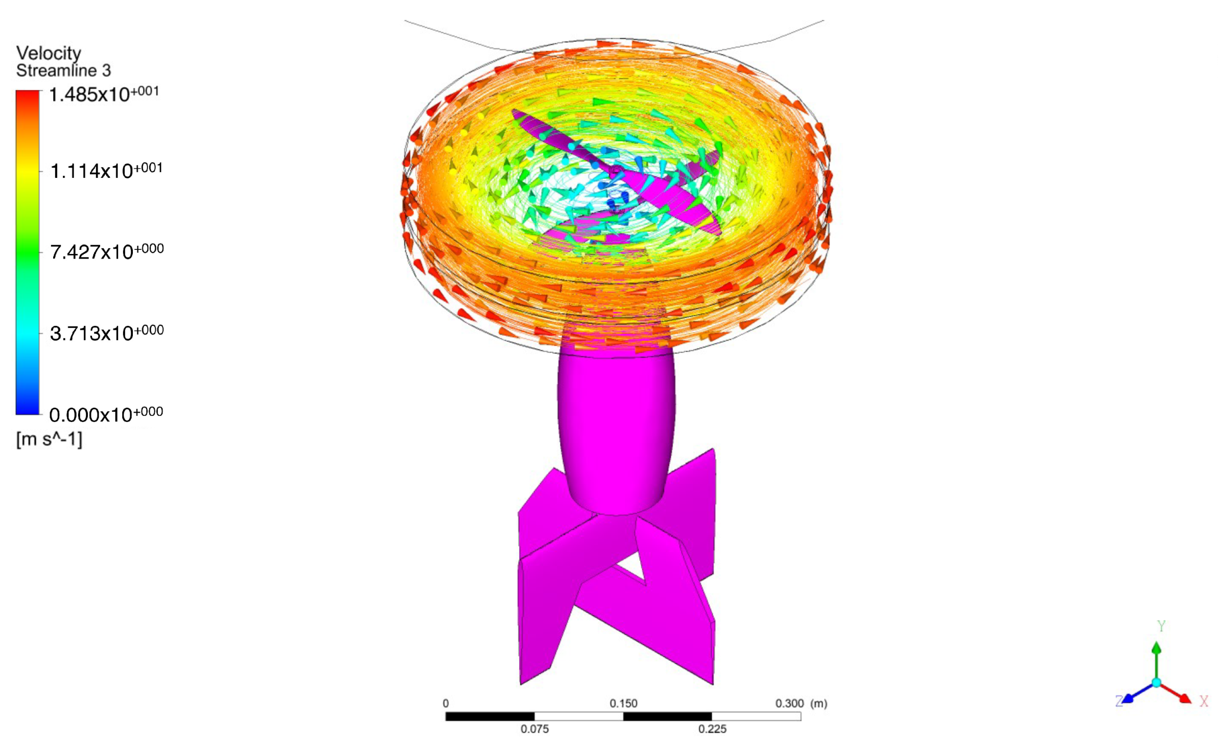
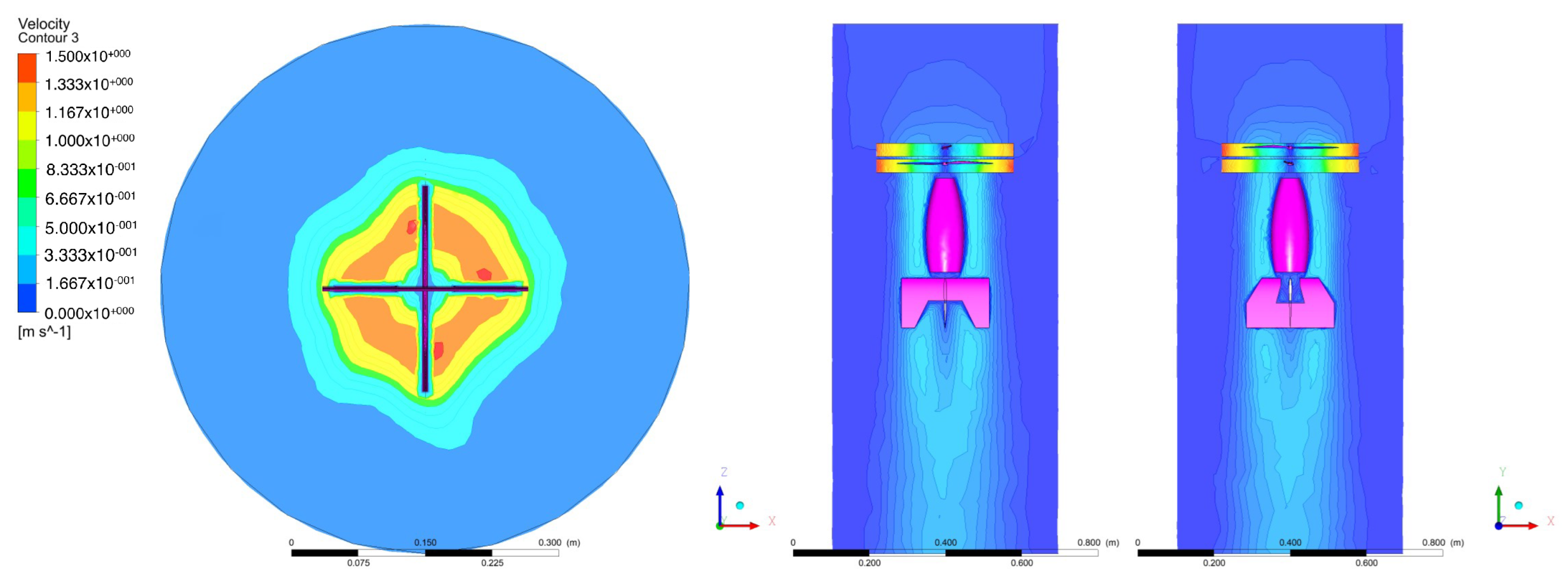
The CFD simulation is obtained for later transient and stationary modes.
3.
The ground testing results are analyzed to validate the proposed computational methodology.
The rest of the paper is organized as follows. Section 2 presents the conceptual design of the micro coaxial rocket UAV (MCR UAV v3.0). Section 3 discusses the CFD simulation of the MCR UAV v3.0 for transient and stationary modes. Section 4 describes the mathematical model using the Newton–Euler formulation to obtain the linear control, while Section 5 provides the results of the UAV from the ground testing. Finally, conclusions are given in Section 6.

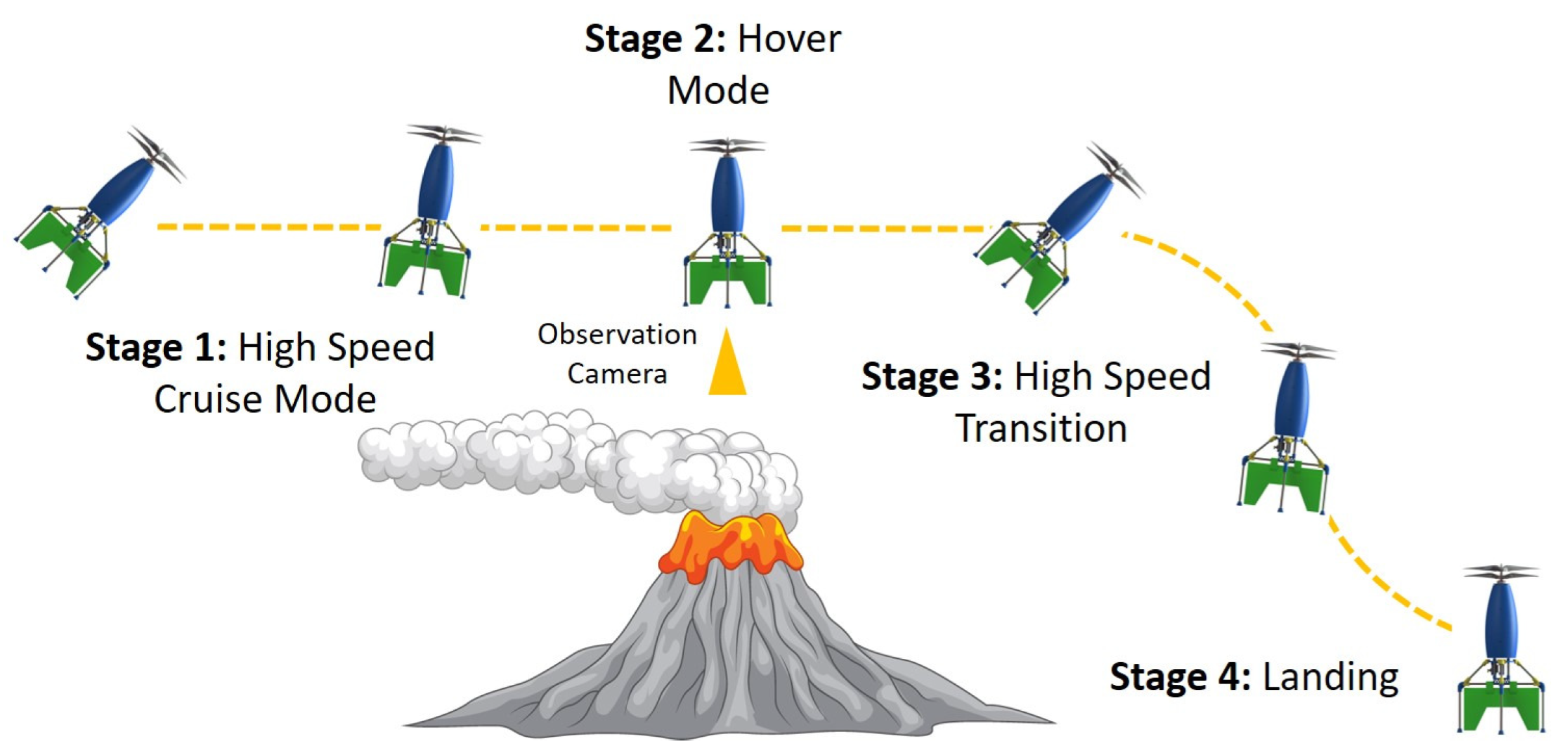
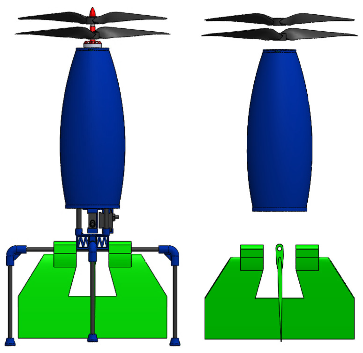
2. Conceptual Design of Micro Coaxial Rocket UAV (MCR UAV v3.0)

The main characteristic of this aerial vehicle is that is capable of performing vertical and hover flight as well as horizontal flight. The main objective of this MCR UAV v3.0 is to enable fixed-wing as well as shuttle operation, then automatic hovering flight once it arrives at the objective where a risk exists for a human being, so that the vehicle can perform monitoring and observation, acquiring and sending data to a ground station using a camera and advanced telemetry (see Figure 1). The proposed methodology for the development of this micro UAV is shown in the following flowchart (see Figure 2).
The MCR UAV consists of two main contra-rotating rotors which provide the vehicle thrust vector, where both are capable of regulating yaw and height motion. It also has two control surfaces or ailerons used to control the vehicle in roll and pitch motion during the flight. Based on the propulsion system capabilities, a contra-rotating brushless motor was used to maintain the micro UAV in a vertical position, and the autopilot was selected based on the vehicle configuration. The fuselage of the vehicle was designed to preserve the autopilot by safely allocating the positions of the electronic components. The fuselage of the vehicle was based on a rocket design of size 225.7 mm to obtain stability in vertical, hover and horizontal flights. The length of the ailerons chord was about 140 mm (see Figure 3).
The autopilot was selected based on the selected propulsion system: CR23L KV1100 with a 9047 CR/CCR propeller. The rotor requires ESCs (electronic speed controllers) capable of maintaining a constant 25A; thus, one AEO E-Power 30A was used for each rotor, and a Pixhawk flight computer with 180 MHz ARM® Cortex was integrated. This computer has an MPU6000 as the IMU, an ST Micro 16-bit barometer and an ST Micro 14-bit magnetometer. In addition, a U-Blox 6 GPS was attached externally. Two Hitec HS65-MG micro servos were used as ailerons. The whole system was controlled by a Spektrum DX8 radio controller (see Table 1).

3. CFD Analysis

Numerical CFD modeling of the MCR UAV was performed using Ansys Fluent and Flow Simulation embedded in CAD-oriented software. To save computational resources, a simplification of the conceptual design was used (see Figure 4) [24,25].
The simplified model was divided into three different control volumes: one for each propeller and another for the entire vehicle. Blade enclosures were excluded from the MCR UAV since these are meshed as a rotating element (see Figure 5).
The first stage of CFD modeling consisted of a transient CFD simulation executed to calculate velocity streams around the ailerons. This information was used as a starting point for a stationary model to calculate the lift and drag coefficients and evaluate the effect of the control surfaces. The ailerons are a secondary source of vehicle transition, and the behavior of the control surfaces is considered critical; thus, a correct prediction of the aerodynamics is essential. The ailerons were subjected to low airstream velocities provided by the two counter-rotating blades, and the rotating elements were not shrouded. As a consequence, low Reynolds Numbers were expected.
For the transient CFD simulation, a pressure-based algorithm and k ϵ turbulence model were selected to solve the second-order equations for incompressible flow. The operation conditions of the MCR UAV were normal atmospheric conditions, since the configuration of a rotatory-wing vehicle is relatively low compared with fixed-wing vehicles. The International Standard Atmosphere (ISA) was used for the boundary conditions at sea level, and it was essential to establish the rotation direction and specific coordinates of the origin of the flow domains. An average angular velocity of 9000 rpm was established for each propeller enclosure in the CFD transient simulation. Hybrid initialization was performed using the vehicle enclosure from the inlet for reference values. The iterations were executed, and 800 steps were defined with a value of 0.1 s. Once the stream velocity was completely defined, the most effective control-surface shape could be obtained by varying a set of aerodynamic parameters of the ailerons, including the chord, span, maximum angle of deflection, total area and sweep angle, for a further stationary CFD analysis. The evaluation process and the computational analysis process were continuously repeated until the dynamic requirements were completely satisfied.
For the steady-state model, Flow Simulation embedded in CAD software was employed, using an inverse engineering procedure from 3D UAV CAD, where a 2D sketch is drawn and modified to obtain a group of coordinates that generates a surface in Fluent. A special surface size is employed to mesh the control surfaces, reducing the element size by up to 0.1 mm. Simulations in 3D were performed to calculate the air distribution around the control surfaces and the force produced by each surface to meet dynamical requirements. The maximum angle of deflection for the ailerons was set to 25 degrees due to the mechanical restrictions. A k ϵ turbulence model with scalable wall functions and ISA air properties was considered for steady modeling (see Table 2).
The numerical modeling results included two control surfaces. The maximum angle of incidence was defined as 25 degrees, calculated based on the dimensions of the control surfaces and mechanical restrictions. A large angle of incidence implies a large aperture in the surface, which decreases the net area and the force produced. For the propulsion system, a transient simulation is fundamental to ensure that the entire computational domain corresponds with the real phenomena. The coaxial configuration of the vehicle consists of two contra-rotating propellers, and the conditions defined in the simulation imply a lower counter-clockwise rotating propeller and a top clockwise rotating propeller (see Figure 6).
The transient simulation allows the stream velocity to be evaluated for a steady analysis and allows the aileron lift and drag forces to be calculated. The main results include a range of velocities from 0 m/s to 14.85 m/s. The maximum velocity is at the propeller tips (see Figure 7).
The transient simulation approximates stream velocities around the control surfaces; thus, a scaling strategy is used, reducing the maximum velocity from 14.84 m/s to 2 m/s. Both propellers’ flow domains are depicted as maximum velocities, since they surpassed the defined scale. The results showed that velocities around the ailerons were from 1 m/s to 1.5 m/s, as shown in Figure 8.
In Figure 9, a refinement of the streamlines around the ailerons can be observed. A plane contour is shown with a scaled maximum velocity of 1.5 m/s. The scaled contour shows that a large amount of air is passing through the control surfaces.
The steady CFD analysis shows a clear pressure gradient for all the angles of deflection, proving the functionality of the surfaces when the airstream impacts upon them. It is expected that the maximum pressure will be found immediately on top of the vehicle fuselage, since there is a completely perpendicular wall against the air flow direction (see Figure 10 and Figure 11).
Since the morphology of the control surfaces was not the same as that of conventional ailerons, lifting line theory could not be used to estimate the lift distribution around the entire area; however, by using computational force reports with each aileron name selection defined in the mesh procedure, it could easily be obtained. The numerical results are shown in tables and graphs for the first aileron and the second aileron, respectively. The CFD simulation showed the largest pressure differential at 80% for both ailerons (see Figure 12 and Figure 13).

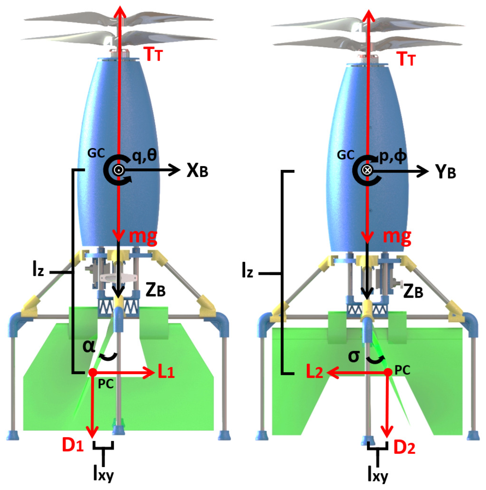
4. Mathematical Model

The model of the MCR UAV v3.0 considers an inertial fixed frame I = { x I , y I , z I } and a fixed body frame attached to the center of gravity of the aircraft B = { x B , y B , z B } . The wind frame W = { x W , y W , z W } is considered during the cruise mode of the airplane [26,27] (see Figure 14).
The equations of motion were obtained by using the Newton–Euler formulation and are given by the following expressions:
ξ ˙ = V
V ˙ = R F + m g e 3
R ˙ = R Ω ^
J Ω ˙ = Ω × J Ω + Γ
where ξ = ( x , y , z ) R 3 and V = ( x ˙ , y ˙ , z ˙ ) R 3 are the position coordinates and the translational velocity relative to the inertial frame. In addition, m R denotes the MCR UAV v3.0 mass, and e 1 , e 2 and e 3 are the vectors of the canonical basis of R 3 in I . Furthermore, e b 1 , e b 2 and e b 3 are the vectors of the canonical basis of R 3 in B , and η = ( ϕ , θ , ψ ) R 3 describes the rotation coordinates, where ϕ , θ and ψ represent the roll, pitch and yaw or the heading, respectively. The rotation matrix, R S O ( 3 ) : B I , satisfies S O ( 3 ) = { R | R R 3 × 3 , det [ R ] = 1 , R R = R R = I } and is parameterized by the Euler angles ϕ , θ and ψ . The rotation matrix is written as:
R = c θ c ψ s ϕ s θ c ψ c ϕ s ψ c ϕ s θ c ψ + s ψ c θ s ψ s ϕ s θ s ψ + c ϕ c ψ c ϕ s θ s ψ c ψ s θ s ϕ c θ c ϕ c θ
Here, Ω = ( p , q , r ) R 3 is the angular velocity in B and Ω ^ denotes the skew-symmetric matrix of the vector which is given by:
Ω ^ = 0 r q r 0 p q p 0
where J R 3 × 3 contains the moments of inertia and Γ = ( Γ x , Γ y , Γ z ) are the moments acting on the drone.

4.1. Forces

The forces acting on the MCR UAV v3.0 are defined as the propulsion, the aerodynamic forces and the weight. The total force is:
F = F x F y F z = F p + F a + F w
The propulsion force of the MCR UAV v3.0 consists of two forces T 1 and T 2 generated by two rotors in a coaxial configuration, as shown in Figure 15.
F p = 0 0 T T
The propulsion thrust force is T T = T 1 + T 2 . The vehicle thrust in B is given by F p = T T e b 3 , assuming that the performance of the upper rotor is not influenced by the lower rotor, that the rotor planes are sufficiently close together and that each rotor provides an equal fraction of the total system [28].
With regard to the aerodynamic forces, the MCR UAV v3.0 was designed with two control surfaces which produce lift L 1 , L 2 and drag D 1 , D 2 forces. This results in:
F a = W L 2 L 1 D 1 + D 2 + D v
with the rotation matrix W S O ( 3 ) : B A that transforms a force from the body frame to the aerodynamic frame described as:
W = c α c β s β s α c β c α s β c β s α s β s α 0 c α
where α is the angle of attack and β is the sideslip angle [28,29].
The weight force is the force due the gravity, given by:
F w = 0 0 m g

4.2. Moments

The moments acting on the aerial vehicle are described as propulsion and aerodynamic moments:
Γ = Γ x Γ y Γ z = Γ r + Γ g + Γ a c + Γ a e
The reaction moment due to the rotor shaft is given by:
Γ r = i = 1 2 Q i ( 1 ) i + 1 e 3 = 0 0 Q T
with Q T = ( Q 1 Q 2 ) for Q i = ρ A i r i 3 c Q i ω i 2 , where ρ is the air density, A i is the rotor disk area, r i is the rotor radius, c Q i denotes the rotor shaft moment coefficient and ω i denotes the angular velocity of the rotor i with i = 1 , 2 .
The gyroscopic moment generated by the rotation of the airframe and the two rotors is described by:
Γ g = i = 1 2 I r i ( Ω × e z ) ( 1 ) i + 1 ω i = Ω 2 ( I r 1 ω 1 I r 2 ω 2 ) Ω 1 ( I r 1 ω 1 + I r 2 ω 2 ) 0
where I r i is the moment of inertia of the rotor i and ω i denotes the angular velocity of the rotor i with i = 1 , 2 .
The actuator moments are generated by the control-surface forces and are described as
Γ a c = L 1 l z + D 1 l x y L 1 l z + D 1 l x y 0
where l z denotes the distance from the center of gravity to the control surfaces through the z axis and l x y denotes the distance between the center of gravity and the control surfaces through the x or y axes. Note that the vehicle is symmetric, so that l x y and l z have the same distance.
Finally, the aerodynamic moments acting on the airframe are described as
Γ a e = L M N
where L , M and N are the aerodynamic rolling, pitching and yawing moments, respectively.
The four independent control inputs, U R 4 in matrix form, provide the following well-posed actuation mapping:
U = A a f
U = 1 0 0 0 0 l z 0 0 0 0 l z 0 0 0 0 1 T T L 1 L 2 Q T
where the mapping A a R 4 × 4 is invertible.

4.3. Equations of Motion

Using Equations(1)–(4), a nonlinear set of equations based on the computed torque can be given:
X ¨ = F x m c θ c ψ + F y m ( s ϕ s θ c ψ c ϕ s ψ ) + F z m ( c ϕ s θ c ψ + s ϕ s ψ )
Y ¨ = F x m c θ s ψ + F y m ( s ϕ s θ s ψ + c ϕ c ψ ) + F z m ( c ϕ s θ s ψ s ϕ c ψ )
Z ¨ = F x m s θ + F y m s ϕ c θ + F z m c ϕ c θ g ϕ ¨ = θ ˙ ψ ˙ c θ + θ ˙ ϕ ˙ s θ c θ + 1 J x x Γ x + q r ( J y y J z z ) + c ϕ s θ c θ J z z Γ z + p q ( J x x J y y )
            + s ϕ s θ c θ J y y Γ y + p r ( J x x J z z )             θ ¨ = ϕ ˙ ψ ˙ c θ + c ϕ J y y Γ y p r ( J x x J z z )
+ s ϕ J z z Γ z p q ( J x x J y y ) ψ ¨ = θ ˙ ϕ ˙ c θ + θ ˙ ψ ˙ s θ c θ + c ϕ c θ J z z Γ z + p q ( J x x J y y )
                    + s ϕ c θ J y y Γ y p r ( J x x J z z )
Remark 1.
In the aerodynamic analysis, the propeller is considered as a disk, and the flow is incompressible. Then, the velocity is constant and the pressure is uniform over the disk.
Remark 2.
The propulsion thrust force T c = T 1 + T 2 , where T 1 = κ w r 1 2 is the upward thrust of the motor and T 2 = κ w r 2 2 is the downward thrust, is generated by the coaxial rotors for an aerodynamic constant κ > 0 . Then, the vehicle thrust in B is given by F p = T T e b 3 , assuming that the performance of the upper rotor is not influenced by the lower rotor. This means that the rotor planes are sufficiently close together and that each rotor provides an equal fraction of the total system.

4.4. Stability Analysis

Considering the approximation of zero Euler angles ϕ = 0 , θ = 0 and ψ = 0 , a simplification of the equations of motion can be performed using Jacobian linearization [30]. The resulting model can be described by:
X ¨ = F x m c θ c ψ
Y ¨ = F y m ( s ϕ s θ s ψ + c ϕ c ψ )
Z ¨ = F z m c ϕ c θ g
ϕ ¨ = θ ˙ ψ ˙ c θ + 1 J x x Γ x + q r ( J y y J z z )
θ ¨ = ϕ ˙ ψ ˙ c θ + c ϕ J y y Γ y p r ( J x x J z z )
ψ ¨ = θ ˙ ϕ ˙ c θ + c ϕ c θ J z z Γ z + p q ( J x x J y y )
These equations can be changed into a state-space form using Euler angles ( ψ , θ , ϕ ) and Euclidean space coordinates (X, Y, Z) as states and forces ( F x , F y , F z ) and moments ( Γ x , Γ y , Γ z ) as inputs. Once the inputs and outputs are stated, state-space matrices are established and converted to transfer functions for frequency domain analysis, to obtain the dynamic requirements using conventional stabilization parameters. The stabilization parameters were defined as time T s = 1.5 s, stationary-state error e ( ) 0 and overshoot M p = 12.5% [31]. Thus, the transfer functions obtained for each of the dynamic requirements of the MCR UAV v3.0 were as follows:
G ( s ) X = 1.199 s 2
G ( s ) Y = 1.199 s 2
G ( s ) Z = 1.199 s 2
G ( s ) ψ = 204.08 s 2
G ( s ) θ = 78.74 s 2
G ( s ) ϕ = 78.74 s 2
A classic control technique was to study and analyze the flight dynamics of the MCR UAV v3.0, and an activation scheme was developed in order to predict the required rotor speed and deflection angles of the control surfaces. This was implemented using a force and moments balance in each axis at the center of gravity, resulting in:
Γ x = L 1 l z + D 1 l x y
Γ y = L 2 l z + D 2 l x y
Γ z = c Q 1 T 1 c Q 2 T 2
F x = L 2
F y = L 1
F z = D 1 + D 2 T 2 T 2
Rewriting the previous set of equations in matrix form, it is possible to obtain the following structure, where the matrix in the middle is called Propulsion Matrix 1 [ M P 1 ] .
Γ x Γ y Γ z F X F y F z = l z 0 l x y 0 0 0 0 l z 0 l x y 0 0 0 0 0 0 c Q 1 c Q 2 0 1 0 0 0 0 1 0 0 0 0 0 1 1 0 0 1 1 L 1 L 2 D 1 D 2 T 1 T 2
Moreover, it is possible to write [ L 1 L 2 D 1 D 2 T 1 T 2 ] as the function of the angular velocities of each rotor:
L 1 = ( α ) ( k L 1 ) ( w r 1 2 + w r 2 2 )
L 2 = ( σ ) ( k L 2 ) ( w r 1 2 + w r 2 2 )
D 1 = ( k D ) ( w r 1 2 + w r 2 2 )
D 2 = ( k D ) ( w r 1 2 + w r 2 2 )
T 1 = ( k ) ( w r 1 2 )
T 2 = ( k ) ( w r 2 2 )
where α and σ represent each angle of deflection of both control surfaces, and k L 1 , k L 2 are the CFD-calculated lift coefficients for each control surface. All the presented equations can be restated in matrix form; however, the [ D 1 D 2 ] expressions are neglected in this procedure. This results in:
T 1 T 2 = k 0 0 k w r 1 2 w r 2 2
L 1 L 2 = ( k L 1 ) ( w r 1 2 + w r 2 2 ) 0 0 ( k L 2 ) ( w r 1 2 + w r 2 2 ) α σ
The middle matrices are denoted Propulsion Matrix 2 [ M P 2 ] and Propulsion Matrix 3 [ M P 3 ] , respectively. It can be observed that the activation scheme was designed by inverting all propulsion matrices; the inverse forms of the matrices allow the required deflection angles of the control surfaces and the angular velocities of each rotor to be calculated (see Figure 16).
Many control approaches have been suggested for similar vehicles in the literature, such as PID, LQR and backstepping. Nonetheless, in this article, the main objective was to approach the vehicle design and control problem from a multidisciplinary point of view, with a particular emphasis on model fidelity. Therefore, a simple root locus control design method was used. The simplicity of this approach also highlights the contribution of the activation scheme in Figure 16, which enables the use of this simple control scheme by successfully decoupling the vehicle dynamics.
According to the proposed stabilization time and overshoot, it is possible to create a second-order ideal closed-loop transfer function where the important element is the denominator. This is called an ideal closed-loop denominator I C L D , where the first-order element contains the damping factor ζ times the undamped oscillation frequency W n times 2, and the independent element is the square of the undamped oscillation frequency (Equation (42)) [30]. The damping factor can be calculated using the required overshoot:
I C L D = s 2 + 5.33 s + 23.34
Obtaining a new second-order function, which is defined as the desired pole for the branches in the root locus diagram, including its roots, gives Equation (43):
S I C L D = 2.66 ± 4.02 j
Considering Equation (22) as an example, and since a constant reference is defined as the input for the control scheme, a simple proportional controller is shown in Equation (44).
C ( s ) = K
Based on linear control theory, which establishes that the difference between the angle summation between zeros γ and poles λ in root locus diagrams give a result of ± 180 , Equation (45) is obtained. This is defined as the phase condition that defines which poles really are on the diagram [30]:
G ( s ) = γ λ = ± 180 ( 2 n + 1 )
According to the root locus plot and the phase condition, the actual branches of the diagram do not intersect the I C L D . As a consequence, the phase condition is not fulfilled with the actual poles. The procedure is performed by calculating the existing angle between the actual transfer function poles (Equation (22)) and the ideal closed-loop denominator poles (Equation (43)). This can be achieved using the arc tangent trigonometric function for each pole, resulting in 123 . 49 for each pole. Substituting the calculated values into the phase condition formula (Equation (45)) results in:
246 . 98 ± 180
To fulfill the phase condition, a new zero γ X term for the controller is required. Adding the new term to the phase condition statement results in Equation (47):
γ X 246 . 98 = ± 180
Equation (47) shows that the new term γ X requires an angle of 66.98 ; therefore, since this term is a non-complex zero, this must be allocated at a real axis. Then, the vertical separation is well known to be 4.02; however, the horizontal separation L between the ideal closed-loop denominator S I C L D and the new non-complex zero is unknown.
The calculation of the horizontal separation L between the new zero and the root of the ideal closed-loop denominator S I C L D pole on the real axis can be calculated using the tangent trigonometric function, marking the adjacent distance as an unknown variable. According to the calculation, this value is 1.67. Since the required angle of 66.98 is acute, the new zero must be allocated on the left of the ideal closed-loop denominator S I C L D pole in the root locus diagram, where the amount of 2.66 is added, resulting in 4.33 for the allocation of the new non-complex zero. This results in a new controller form that includes the new zero in the numerator.
C ( s ) = ( s + 4.33 ) K 1
In essence, this controller is not a proper function, and therefore a non-dominant pole is also required. This must be a minimum of 10 times faster than the real part of S I C L D [30]. This gives:
C ( s ) = ( s + 4.33 ) K ( s + 26.6 )
The addition of a non-dominant pole affects the already calculated phase condition (Equation (47)), resulting in complete reprocessing to modify the real value of the added zero. This results in Equation (50):
C ( s ) = ( s + 5.22 ) K ( s + 26.6 )
At this point, it branches from the transfer function across S I C L D at the root locus, but the value of K and what it does is unknown. The gain margin formulation (Equation (51)) is used to obtain this value, giving a result of 93.32.
K = 1 G ( s ) C ( s ) s = S I C L D
C ( s ) = ( s + 5.22 ) 93.32 ( s + 26.6 )
Note that this process was performed for all transfer functions obtained from the equations of motion, to obtain the dynamic requirements for a posterior CFD validation. Since the vehicle preserves a symmetric configuration along the X and Y axes, only a single simulation was developed to obtain the dynamical requirements.
The control technique and linearized vehicle dynamics were added to activate the scheme previously elaborated, giving, as a result, the entire vehicle control scheme (see Figure 17).

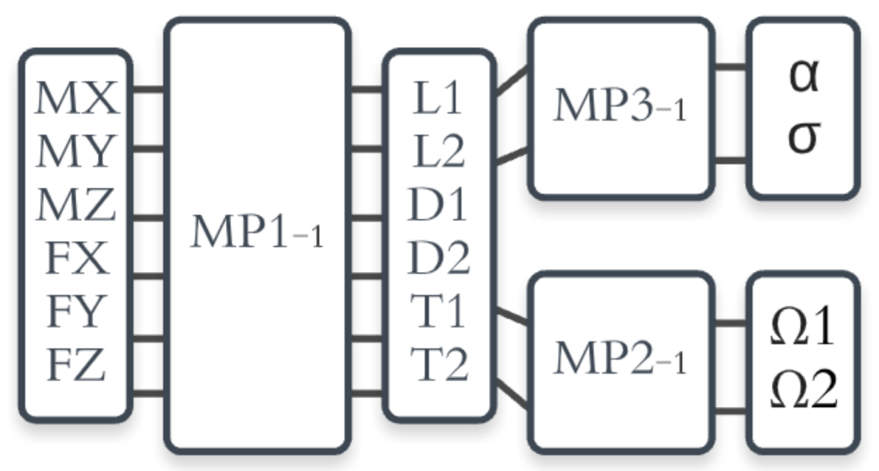
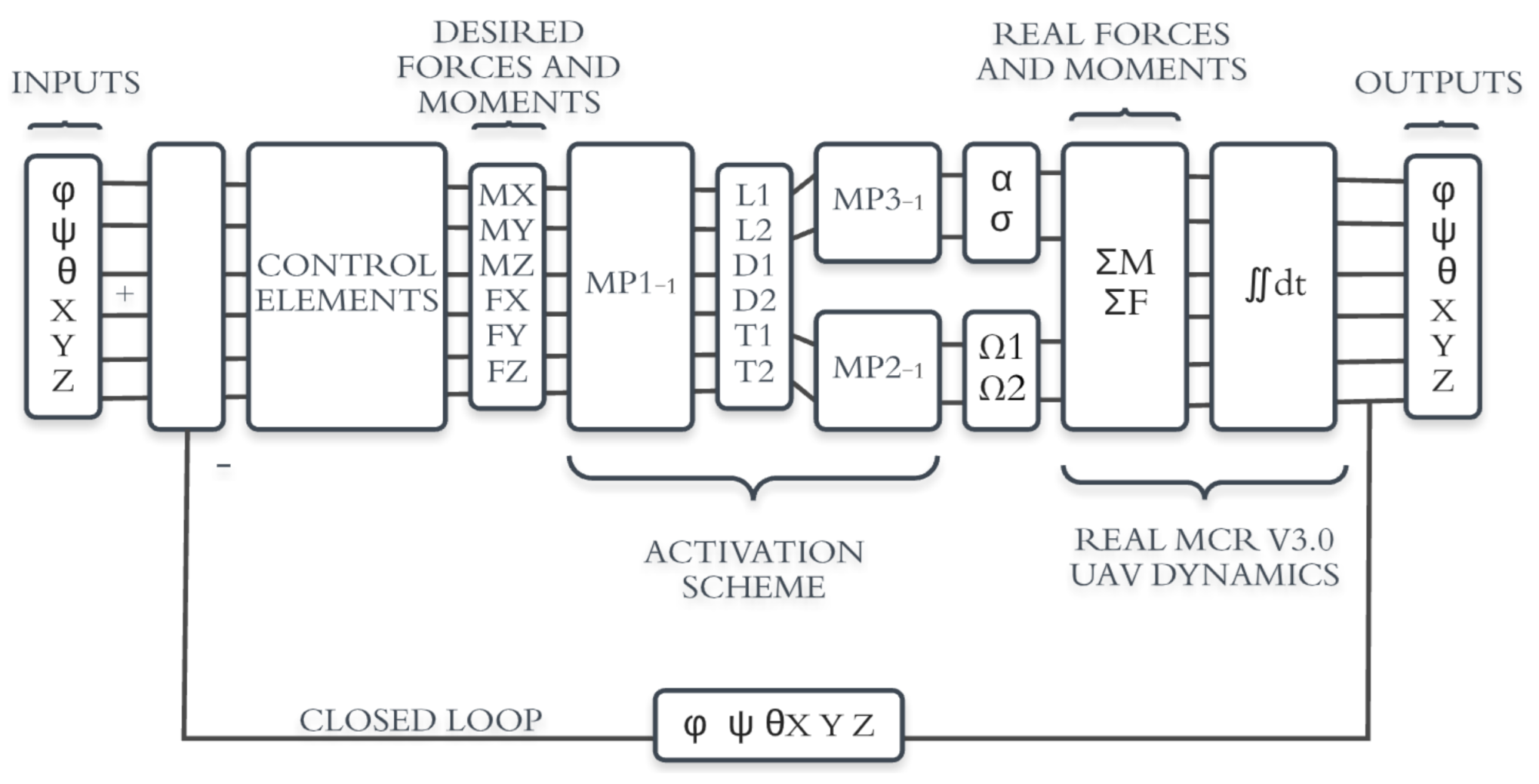
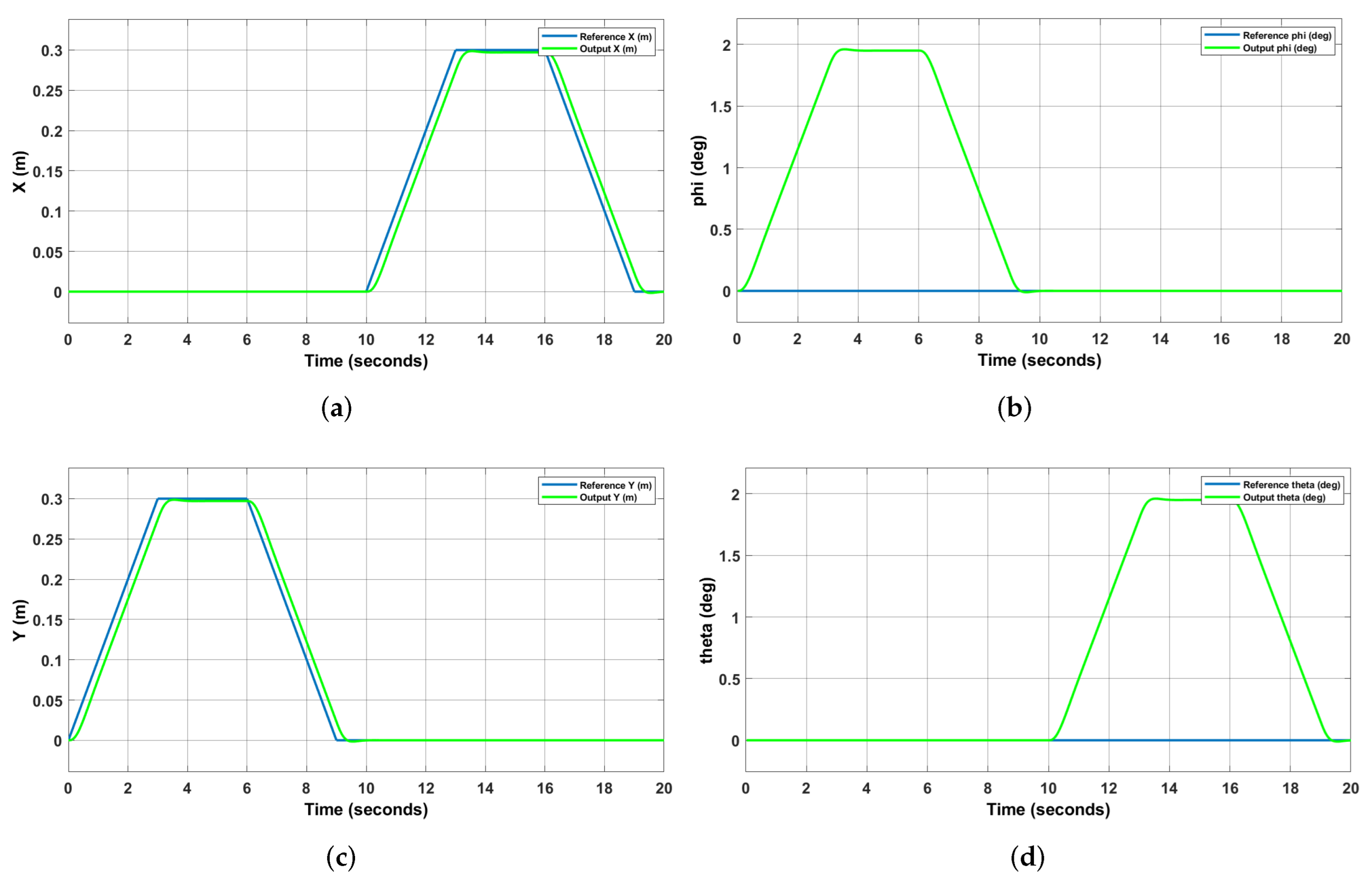
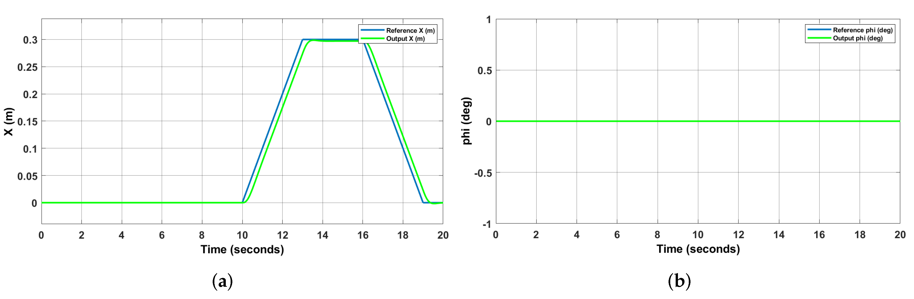
4.5. Simulation Results
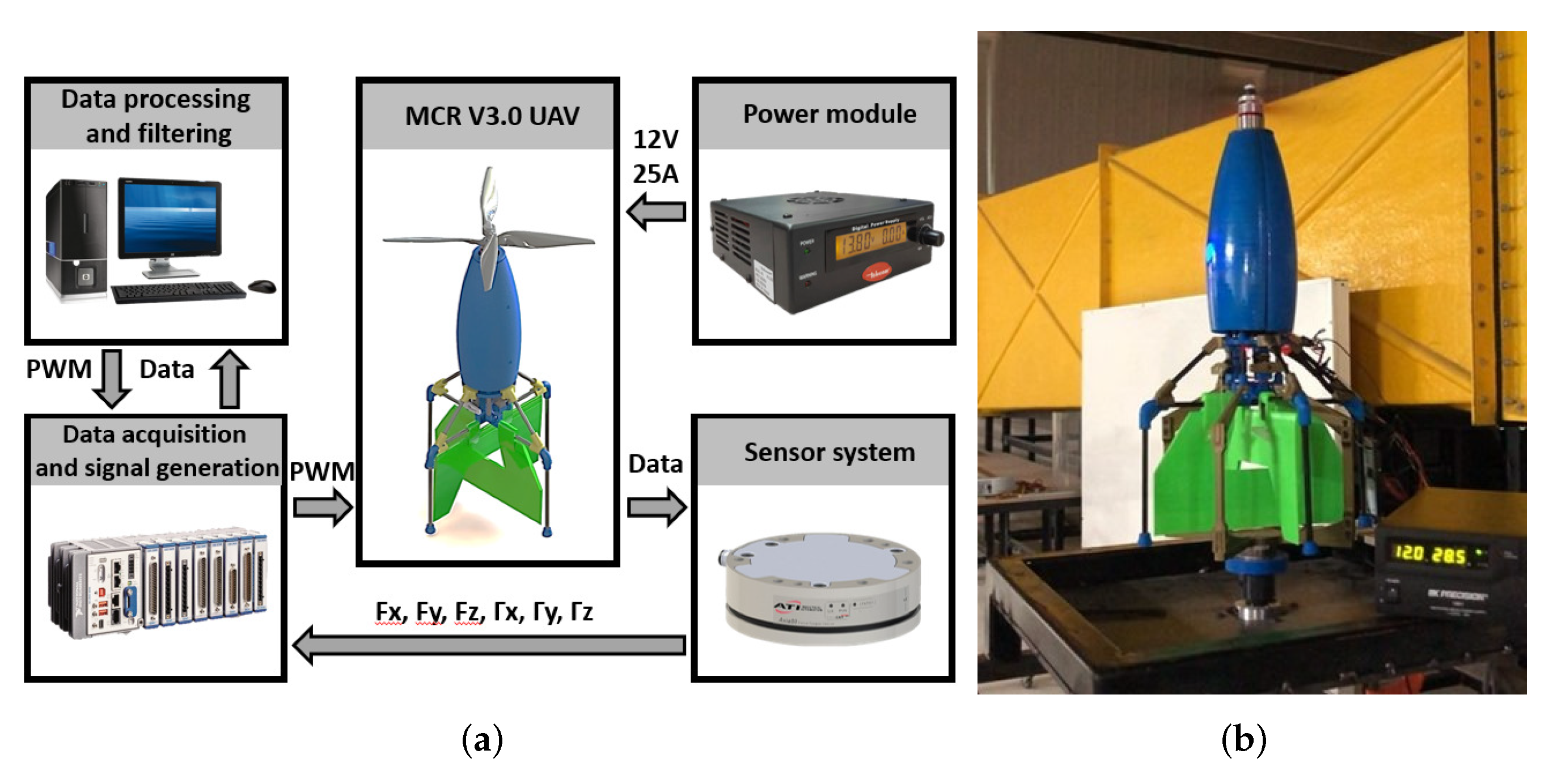
Numerical simulations were run using MATLAB software (version 2018b) to validate the proposed modeling and linear control. For this purpose, a constant input of 0.5 m was selected for the altitude Z to obtain the dynamic requirement for the vehicle. The force magnitude required for a maneuver to reach an altitude was about 3.37 N, which is within the thrust value of the contra-rotating rotors, i.e., 8.33 N (see Figure 18). This figure shows the output response, which performs the desired behavior when the control parameters are fulfilled. In effect, the rotor capabilities are good enough to give a settlement time of less than 1.5 s and an overshoot of less than 20%.
A pre-filtered input was used in the ϕ transfer function to obtain a response with an overshoot of less than 20% and a stabilization time of less than 1.5 s (Figure 19). The moment response is illustrated in Figure 19, and it shows that the moment required to handle the most aggressive maneuver required was about 0.035 Nm, which is within the range previously established by the capabilities of the control surfaces.
The next procedure involved a set of numerical simulations in which a pre-programmed signal was used as an input for the translational dynamics (X, Y, Z) and yaw angle ( ψ ). It should be mentioned that all the reference values of the simulation were properly designed for the MCR UAV v3.0 capabilities. These included a maximum angle of deflection for both ailerons of 25 degrees and a maximum thrust provided by each rotor of 8.3 N. Moreover, with the aim of assuring the stability of the vehicle, the final output must fulfill two different criteria in order to be considered acceptable: an overshoot of less than 12% and a stabilizing time of less than 1.5 s.
The first simulation only included a sinusoidal input in Z, with an amplitude of 1 m and a frequency of 1 rad/s. Other coordinate ( X Y ) references were neglected in this simulation because the purpose was to evaluate the stability of the vehicle’s altitude. In this sense, the rotational dynamics ( ϕ , θ , ψ ) were zero signals, also caused by the lack of X Y input. The thrust for each rotor ( T 1 , T 2 ) and the angles of deflection ( σ , α ) were calculated, as well as the dynamic responses. Unsurprisingly, the thrust response showed a sinusoidal signal similar to that of the altitude response, matching the peaks and the lowest points of the signal. The force required could be provided by the coaxial rotors. The ailerons’ angles of deflection were zero, as for the rotational dynamics in Figure 20.
The second simulation included a sinusoidal signal with the same amplitude and frequency on the same axis. Moreover, in the XY coordinates, a positive displacement of 0.3 m was demanded in a time of 3 s generating a smooth path, remaining at that position for 3 s and returning to the origin. It is important to mention that, applying the same trajectory used to reach 0.3 m, the path described was executed in different time periods for each coordinate.
The results show an accurate response for the XY trajectories, with an overshoot of less than 20% and a stabilization time of less than 1.5 s. However, for the altitude response, a higher overshoot was observed, which is attributed to the thrust vector decomposition when a trajectory is demanded for other longitudinal coordinates. The rotational dynamics values show a natural response in ϕ and θ angles, reaching a maximum point of 2 degrees each, not considered as an elevated angle for this type of coaxial configuration. Furthermore, the thrust response shows a sinusoidal signal highly similar to the altitude input. Nevertheless, fluctuations across the response are visible, caused by the additional force required to accomplish the XY paths. The angle deflections obtained were within the MCR UAV v3.0 mechanical operation range, with a change in aileron deflections requested precisely at each change of trajectory (XY) (see Figure 21).
An accurate response for the X coordinate was obtained, fulfilling the overshoot and stabilization time conditions, and the Y output was a zero signal, since a trajectory was not demanded. The altitude response can be divided into two different parts, each taking 10 s. Firstly, the signal response corresponds well to the sinusoidal input during the initial part, accomplishing the stability requirements. However, the second part shows a higher overshoot. As expected, the rotational dynamics shows a unique response for the θ angle, with the same magnitude as that presented in Figure 21. Furthermore, the thrust response shows a similar behavior to the Z output, including a sine wave signal in the first instance. Nevertheless, after 10 s, fluctuations are observed, and these are attributed to an excess thrust requirement. The deflection angles do not surpass the MCR UAV V3.0 mechanical capabilities, reaching a maximum of 23 degrees (see Figure 22).

5. Ground Testing

The quantification of a methodology that involves several fields of study working together with a specific purpose creates a high-level technique that can be used in non-conventional UAV design. In this part of the study, a series of experiments were carried out as flight statics to obtain performance data for the vehicle, considering the avionics system, structural elements, ailerons, propulsion system and power modules.
The platform used coaxial rotors as a propulsion system. The avionics consisted of a Pixhawk autopilot and two servos for the ailerons of the vehicle [32]. The autopilot processes the data acquired from the sensors and RC inputs, then the control algorithms are executed in order to calculate the command signals, which are sent to the servos and the brushless motor. The GPS provides the position and the speed signals for the translational coordinates. The MCR UAV communicated via wireless to the ground station using telemetry modules which served as a receiver and transceiver. A LiPo battery was used as a power supply and the Spektrum DX8 radio controller was used for manual mode if required. Note that the firmware of the Pixhawk autopilot was modified for our aerial vehicle.
Lightweight metals, composites and high strength polymers are materials widely used in aeronautical applications for various purposes. The MCR UAV v3.0 was mainly built using fused deposition molding (FDM) as the main manufacturing technique, including an MC3D ABS filament. The main parameters of the components and control surfaces were based on the manufacturing theory. Tri-hexagon infill was used for the platform elements and gyroid infill for the ailerons, since these elements require a large plastic deformation [33]. Furthermore, structural elements were principally composed of 7 mm diameter glass-fiber tubes attached to each other with 3M epoxy glue, and nylon screws were used in structural joints and the structural surface joint at the top of the vehicle to reduce the total weight.

5.1. Test Bench

Since the main purpose of the coaxial rotors in hover flight is to provide a vertical lifting force in opposition to the weight of the UAV, the propulsion system was characterized. In this sense, it was proposed to measure the complete propulsion system, including both rotors spinning at the same time along with the control surfaces acting at different angles. This methodology allowed a realistic environment to be used to identify the particular forces and moments produced by the propulsion system. In effect, ground testing allowed the visualizing and measurement of phenomena such as the interaction between the propellers, the interaction with the bullet frame of the vehicle, the power electronics and the autopilot. Since a large number of data points are required to characterize the MCR UAV v3.0, quantifying the forces and moments produced by the actuators, it is possible to determine the capabilities of the vehicle for navigating in real time.
In order to measure the actual forces and moments produced by the propulsion system and to consider the wind effect on the propeller frame, a test bench was implemented in a controlled environment. Ground testing was performed statically, and the vehicle was completely attached to a structure with a strain gauge, designed so that it affected, as a minimum, the air path and the control surfaces deflection. The test bench used for the experiments consisted of a data acquisition system from National Instruments with the following components: cRIO-9035 chassis, 2 NI 9215 analog input modules and 1 NI 9361 digital counter module for duty-cycle measurement. The data were obtained at a sampling rate of 20 kHz, and the six-axis load cell system possessed the following resolution ratings: F x = 1/100 N, F y = 1/100 N, F z = 1/50 N, Γ x = 1/4000 N·m, Γ y = 1/4000 N·m and Γ z = 1/4000 N·m. The computational system used for ground testing was dedicated to the processing/filtering and analysis of the data obtained from the load cell and the data acquisition system. The equipment used was a Dell OptiPlex 3040, with the following characteristics: Intel Core i5-6500 SFF 3.2 GHz, 8 GB DDR3L SDRAM, 500 GB HDD, Intel HD Graphics 530 graphics unit.
Firstly, a PWM time-varying input signal was used to control the position of the ailerons using five time-steps of three seconds each. As a consequence, the aileron changed its position by 5 degrees in every time-step, starting from 0 degrees. This task was developed using a programmed script in MATLAB. Secondly, the propulsion system was required to provide enough thrust to overcome the weight of the MCR UAV v3.0; that is, all the data acquisition was performed in hover conditions. This task was achieved using an external power source capable of providing the cuurent and voltage and holding them constant for a longer time than a common LiPo battery. Moreover, once the programmed PWM signal for both servomotors was online and the MCR UAV v3.0 weight was overcome, the acquisition data algorithm could be executed. This algorithm was used to measure the data, using the load cell in combination with the posterior signal processing and filtering. Note that MCR UAV V3.0 inputs are based on a PWM signal and the required power to the main rotor. The outputs of the ground testing system are the forces and moments for every axis (Figure 23).

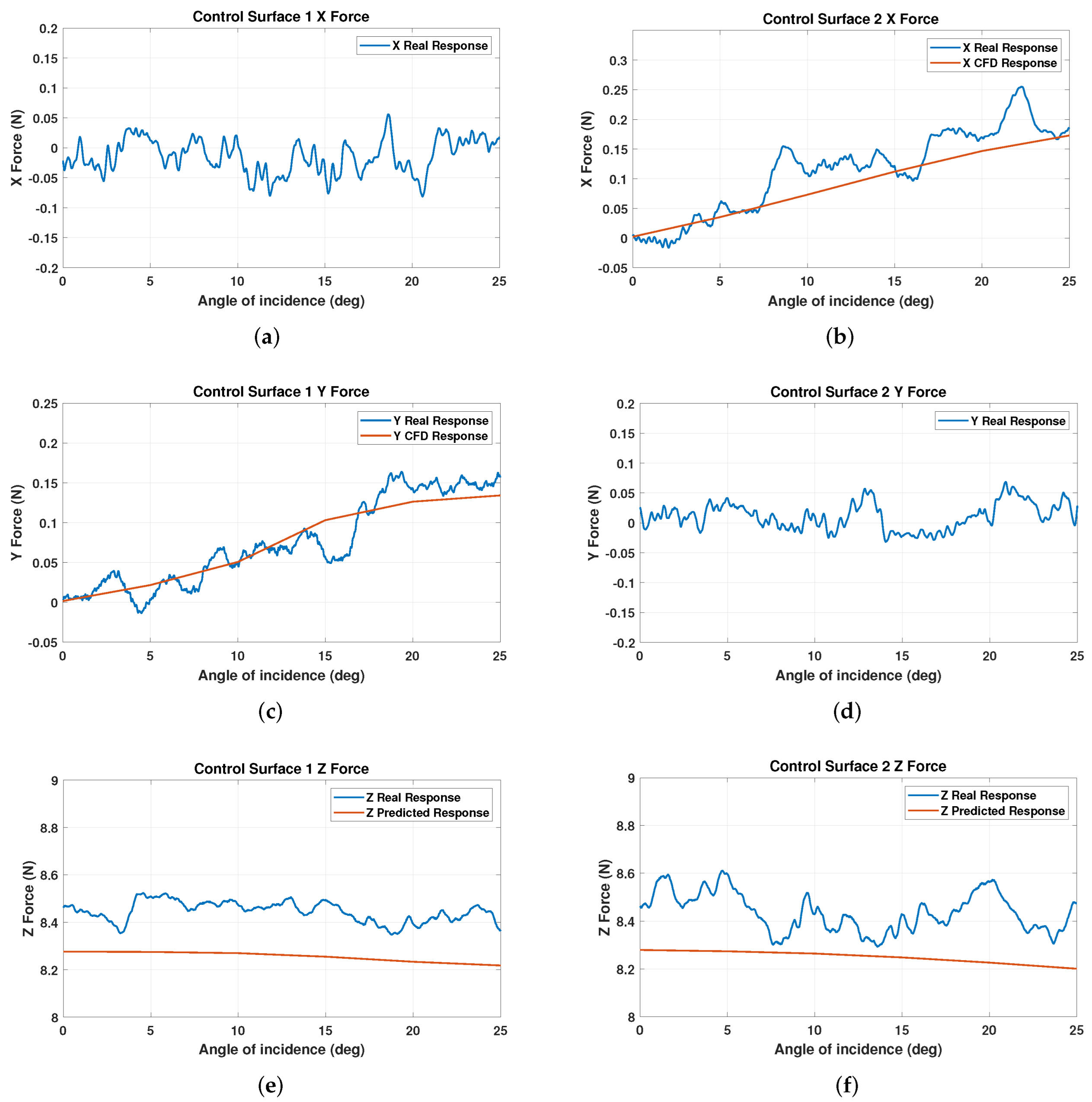
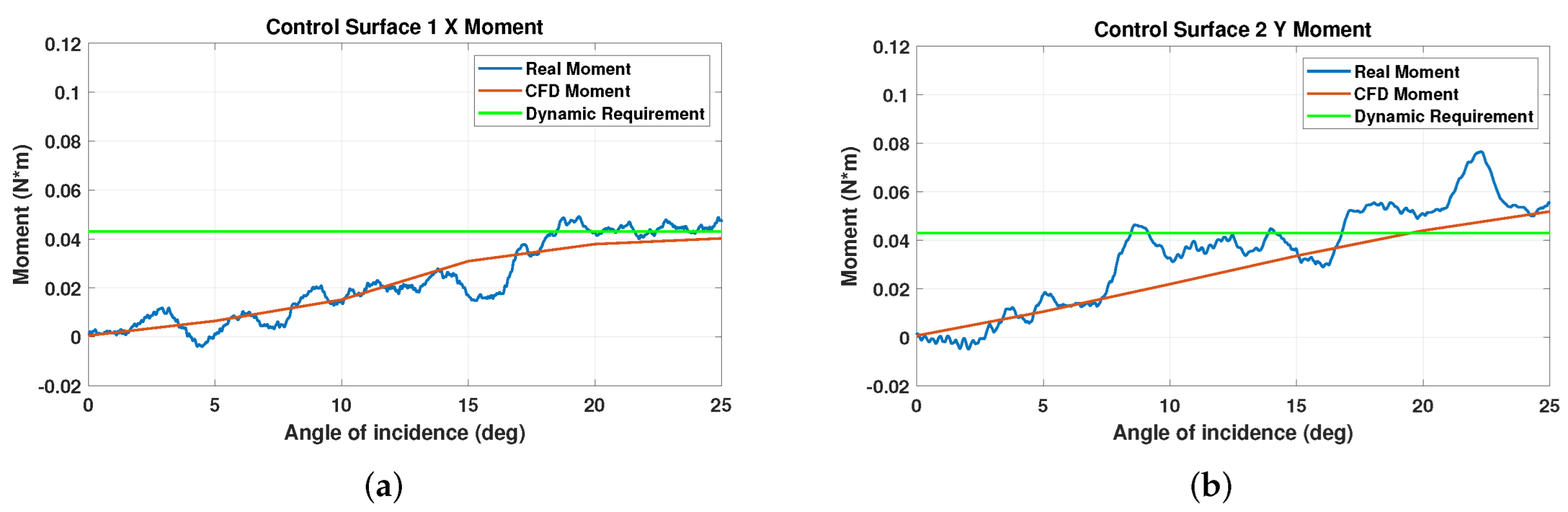
5.2. Comparison of Results

To calculate the real force produced by both ailerons, two different requirements must be fulfilled. Firstly, a PWM time-varying input signal was used to control the position of the ailerons, using five time-steps of five seconds each. As consequence, the ailerons changed their positions by 5 degrees in every time-step, starting from 0 degrees. Secondly, the thrust was required to be enough to overcome the weight of the MCR UAV v3.0. This means that all the data acquisition occurred in the hover condition. Once both conditions were met, it was possible to begin the procedure. However, signal noise, vibration, temperature and external disturbances can cause failures in data acquisition, and these specific issues meant that it was necessary to repeat the procedure until acceptable data were obtained.
Figure 24 shows the forces obtained from the sensor for every axis for both procedures, adding the CFD results for the specific axis where the ailerons generate a force. The first aileron procedure shows a signal approximating to 0 N, since no force is acting on the X axis. However, the Y axis has a force acting on it, attributed to Aileron 1. On this axis, a smooth behavior is observed, with no noise spikes, and both scales show similar standard deviations of 0.0016 N and 0.0043 N as minimum points and 0.134 N and 0.149 N as maximum points from the computational and experimental results, respectively. A Z-axis comparison, subtracting the vehicle weight, was performed between the experimental data and the force obtained from the CFD. Table 3 shows the first aileron results numerically. The second aileron procedure gives the response for the X axis, where a force is acting, and it shows similar signals to those of the first aileron Y-axis response. The Y-axis response shows a signal approximating to 0 N, which is acceptable, and the Z-axis comparison was performed using the same methodology. For Aileron 1, this showed a differential of 0.2 N on average. Table 4 shows the second aileron results numerically (see Figure 24). As a way to enhance the reliability of the results obtained from both strategies, the standard deviation S D was used. The main equation that describes this parameter is defined in Equation (53).
S D = κ μ 2 N
where κ is some value of the data series, μ is defined as the average data value and N is the number of values belonging to the data series.
A surface graphic was used to illustrate the forces obtained for both ailerons on their respective actuating axes (Figure 25). This was performed using the time and deflection angle for X and Y, respectively, whereas Z was used to present the force magnitude. Aileron 1 shows a constant behavior below 20 degrees of deflection; after that point, the force is abruptly increased. Moreover, Aileron 2 shows a non-smooth behavior; however, this can be attributed to noise spikes.
Using the distance from the center of gravity of the MCR UAV v3.0 to the ailerons’ pressure centers (0.30 m) and the forces obtained, it is possible to estimate the momentum of the vehicle and make comparisons regarding the CFD simulation, the experimental platform and the dynamic requirements. Figure 26 shows that the actual surfaces are capable of covering the dynamic requirements provided by the vehicle dynamics, established as 0.043 Nm; however, comparing the actual results from CFD simulations and the experimental data, it can be seen that the experimental data only just meet dynamic requirements. Thus our proposed methodology is feasible. Table 5 and Table 6 show the MCR UAV v3.0 moment results numerically.
A link to a video about our proposed methodology involving flight dynamics, simulation and ground testing can be found at https://youtu.be/iJeO0dtM5ew (accessed on 22 March 2022).

6. Conclusions

This paper described the complete conceptual design of a novel micro coaxial unmanned aerial vehicle (MCR UAV v3.0), encompassing flight dynamics, CFD and linear control theory. The CFD results were obtained for transient and stationary conditions, which provided airstream velocities and aerodynamic forces. Considering the CFD simulation, an iterative process was performed to achieve the dynamical requirements, i.e., the forces and moments required to find suitable control surfaces for the UAV. In effect, the vehicle was mathematically modeled using the Newton–Euler formulation. It was linearized, simulated and validated in a closed loop, along with linear control. The comparison between the CFD simulation and experimental results from the ground testing showed a resemblance in the various aileron angles of deflection, proving the accuracy of both procedures and including a set of parameters, environmental conditions and reference values for the fluid analysis. In addition, by contrasting the experimental and computational responses with the dynamical requirements obtained from the MCR UAV v3.0 dynamics, it was possible to observe that both results just satisfied the calculated dynamic prerequisites and did not surpass the control surfaces’ mechanical restrictions. Finally, the results demonstrated that the proposed methodology was feasible and accurate.

Author Contributions

Conceptualization, V.H.D.; methodology, O.G.-S.; software, V.H.D. and L.A.R.-O.; validation, V.H.D. and L.A.-B.; formal analysis, V.H.D. and O.G.-S.; investigation, V.H.D. and O.G.-S.; resources, O.G.-S., L.A.-B. and L.A.R.-O.; data curation, C.S.-D. and E.G.R.-R.; writing—original draft preparation, V.H.D.; writing—review and editing, V.H.D. and O.G.-S.; visualization, E.G.R.-R. and C.S.-D.; supervision, O.G.-S.; project administration, O.G.-S.; funding acquisition, O.G.-S. All authors have read and agreed to the published version of the manuscript.

Funding

This research was supported by the Office of Naval Research Global through grant number N62909-20-1-2030.

Funding

This research was supported by the Office of Naval Research Global through grant number N62909-20-1-2030.

Institutional Review Board Statement

Not applicable.

Informed Consent Statement

Not applicable.

Data Availability Statement

The data presented in this study are available on request from the corresponding author.

Acknowledgments

The authors would like to thank the Office of Naval Research Global for support through grant number N62909-20-1-2030.

Conflicts of Interest

The authors declare no conflict of interest.

References

  1. Paulos, J.; Yim, M. Flight performance of a swashplateless micro air vehicle. In Proceedings of the 2015 IEEE International Conference on Robotics and Automation (ICRA), Seattle, WA, USA, 26–30 May 2015; pp. 5284–5289. [Google Scholar]
  2. Carholt, O.C.; Fresk, E.; Andrikopoulos, G.; Nikolakopoulos, G. Design, modelling and control of a single rotor UAV. In Proceedings of the 24th Mediterranean Conference on Control and Automation (MED), Athens, Greece, 21–24 June 2016; pp. 840–845. [Google Scholar]
  3. Joel, N.C.; Djalo, H.; Aurelien, K.J. Robust control of UAV coaxial rotor by using exact feedback linearization and PI-observer. Int. J. Dyn. Control 2019, 7, 201–208. [Google Scholar] [CrossRef]
  4. Malandrakis, K.; Dixon, R.; Savvaris, A.; Tsourdos, A. Design and Development of a Novel Spherical UAV. IFAC-PapersOnLine 2016, 49, 320–325. [Google Scholar] [CrossRef]
  5. Lee, S.J. Modeling of real-time flight control system for small coaxial helicopter. In Proceedings of the 2014 IEEE Aerospace Conference, Big Sky, MT, USA, 1–8 March 2014. [Google Scholar]
  6. Drouot, A.; Richard, E.; Boutayeb, M. Hierarchical backstepping-based control of a Gun Launched MAV in crosswinds: Theory and experiment. Control Eng. Pract. 2014, 25, 16–25. [Google Scholar] [CrossRef]
  7. Mokhtari, M.R.; Cherki, B.; Braham, A.C. Disturbance observer based hierarchical control of coaxial-rotor UAV. ISA Trans. 2017, 67, 466–475. [Google Scholar] [CrossRef] [PubMed]
  8. Song, Z.; Sun, K. Adaptive fault tolerant control for a small coaxial rotor unmanned aerial vehicles with partial loss of actuator effectiveness. Aerosp. Sci. Technol. 2019, 88, 362–379. [Google Scholar] [CrossRef]
  9. Fan, W.; Xiang, C.; Najjaran, H.; Wang, X.; Xu, B. Mixed adaptive control architecture for a novel coaxial-ducted-fan aircraft under time-varying uncertainties. Aerosp. Sci. Technol. 2018, 76, 141–154. [Google Scholar] [CrossRef]
  10. Wang, Y.; Song, H.; Li, Q.; Zhang, H. Research on a full envelop controller for an unmanned ducted-fan helicopter based on switching control theory. Sci. Technol. 2019, 62, 1837–1844. [Google Scholar] [CrossRef]
  11. Li, J.; Yang, Q.; Sun, Y. Robust State and Output Feedback Control of Launched MAVs with Unknown Varying External Loads. J. Intell. Robot. Syst. 2018, 92, 671–684. [Google Scholar] [CrossRef]
  12. Koehl, A.; Rafaralahy, H.; Boutayeb, M.; Martinez, B. Aerodynamic modelling and experimental identification of a coaxial-rotor uav. J. Intell. Robot. Syst. 2012, 68, 53–68. [Google Scholar] [CrossRef]
  13. Vogeltanz, T. Conceptual design and control of twin-propeller tail-sitter mini-UAV. CEAS Aeronaut. J. 2019, 10, 937–954. [Google Scholar] [CrossRef]
  14. Kim, Y.T.; Park, C.H.; Kim, H.Y. Three-dimensional CFD investigation of performance and interference effect of coaxial propellers. In Proceedings of the 2019 IEEE 10th International Conference on Mechanical and Aerospace Engineering (ICMAE), Brussels, Belgium, 22–25 July 2019; pp. 376–383. [Google Scholar]
  15. Wei, Y.; Deng, H.; Li, K.; Xiong, H.; Jiang, M. Experimental investigation of aerodynamic characteristic for a coaxial rotor aircraft. In Proceedings of the 2020 3rd International Conference on Unmanned Systems (ICUS), Harbin, China, 27–28 November 2020; pp. 251–257. [Google Scholar]
  16. Lei, Y.; Ye, Y. Aerodynamic Characteristics of a Hex-Rotor MAV With Three Coaxial Rotors in Hover. IEEE Access 2020, 8, 221312–221319. [Google Scholar] [CrossRef]
  17. Xu, H.; Ye, Z. Numerical Simulation of Unsteady Flow Around Forward Flight Helicopter with Coaxial Rotors. Chin. J. Aeronaut. 2011, 24, 1–7. [Google Scholar] [CrossRef] [Green Version]
  18. Deng, J.; Fan, F.; Liu, P.; Huang, S.; Lin, Y. Aerodynamic characteristics of rigid coaxial rotor by wind tunnel test and numerical calculation. Chin. J. Aeronaut. 2019, 32, 568–576. [Google Scholar] [CrossRef]
  19. Han, H.; Xiang, C.; Xu, B.; Yu, Y. Experimental and computational analysis of microscale shrouded coaxial rotor in hover. In Proceedings of the 2017 International Conference on Unmanned Aircraft Systems (ICUAS), Miami, FL, USA, 13–16 June 2017; pp. 1092–1100. [Google Scholar]
  20. Bondyra, A.; Gardecki, S.; Gasior, P.; Giernack, W. Performance of coaxial propulsion in design of multi-rotor UAVs. In Challenges in Automation, Robotics and Measurement Techniques; Szewczyk, R., Zieliński, C., Kaliczyńska, M., Eds.; Springer: Cham, Switzerland, 2016; Volume 440. [Google Scholar]
  21. Wang, F.; Jinqiang, J.; Chen, B.M.; Lee, T.H. Flight dynamics modeling of coaxial rotorcraft UAVs. In Handbook of Unmanned Aerial Vehicles; Valavanis, K., Vachtsevanos, G., Eds.; Springer: Dordrecht, The Netherlands, 2015. [Google Scholar]
  22. Espinoza, E.S.; Garcia, O.; Lugo, I.; Ordaz, P.; Lozano, R.; Malo, A. Micro-Helicopter for Long-Distance Missions: Description and Attitude Stabilization. J. Intell. Robot. Syst. 2012, 70, 151–163. [Google Scholar] [CrossRef]
  23. Chauffaut, C.; Escareno, J.; Lozano, R. The Transition Phase of a Gun Launched Micro Air Vehicle. J. Intell. Robot. Syst. 2013, 70, 119–131. [Google Scholar] [CrossRef]
  24. ANSYS. ANSYS Fluent Theory Guide; ANSYS Inc.: Canonsburg, PA, USA, 2013. [Google Scholar]
  25. Anderson, J.D., Jr. Fundamentals of Aerodynamics, 5th ed.; McGraw-Hill Co.: New York, NY, USA, 2010. [Google Scholar]
  26. Stengel, R.F. Flight Dynamics; Princeton University Press: Princeton, NJ, USA, 2004. [Google Scholar]
  27. Stevens, B.L.; Lewis, F.L. Aircraft Control and Simulation; John Wiley and Sons: Hoboken, NJ, USA, 1992. [Google Scholar]
  28. Leishman, J.G. Principles of Helicopter Aerodynamics; Cambridge University Press: New York, NY, USA, 2006. [Google Scholar]
  29. Kermode, A.C. Mechanics of Flight, 11th ed.; Pearson Prentice-Hall: Harlow, UK, 2006. [Google Scholar]
  30. Chen, C.-H. Linear System Theory and Design, 3rd ed.; Oxford University Press: New York, NY, USA, 1998. [Google Scholar]
  31. Cook, M.V. Flight Dynamics Principles; Butterworth-Heinemann: Oxford, UK, 2007. [Google Scholar]
  32. You, W. Pixhawk Users Manual; Getech Ltd.: Ipswich, UK, 2015. [Google Scholar]
  33. Pecho, P.; Ažaltovič, V.; Kandera, B.; Bugaj, M. Introduction study of design and layout of UAVs 3D printed wings in relation to optimal lightweight and load distribution. Transp. Res. Procedia 2019, 40, 861–868. [Google Scholar] [CrossRef]
Figure 1. MCR UAV v3.0 main objective.
Aerospace 09 00245 g001
Figure 2. Flowchart used for MCR UAV v3.0 design.
Aerospace 09 00245 g002
Figure 3. MCR UAV v3.0 dimensions.
Aerospace 09 00245 g003
Figure 4. MCR UAV v3.0 simplified model for CFD analysis.
Aerospace 09 00245 g004
Figure 5. MCR UAV v3.0 meshing of different control volumes.
Aerospace 09 00245 g005
Figure 6. MCR UAV v3.0 velocity streamlines.
Aerospace 09 00245 g006
Figure 7. MCR UAV v3.0 velocity streamlines.
Aerospace 09 00245 g007
Figure 8. MCR UAV v3.0 scaled streamlines.
Aerospace 09 00245 g008
Figure 9. MCR UAV v3.0 velocity-scaled contours.
Aerospace 09 00245 g009
Figure 10. Pressure contours generated for MCR UAV v3.0 with a control-surface angle of deflection from 5 to 25 degrees for Aileron 1.
Aerospace 09 00245 g010
Figure 11. Pressure contours generated for MCR UAV v3.0 with a control-surface angle of deflection from 5 to 25 degrees for Aileron 2.
Aerospace 09 00245 g011
Figure 12. Pressure contours generated for an 80% MCR UAV v3.0 control-surface chord with angles of deflection from 5 to 25 degrees for Aileron 1.
Aerospace 09 00245 g012
Figure 13. Pressure contours generated for an 80% MCR UAV v3.0 control-surface chord with angles of deflection from 5 to 25 degrees for Aileron 2.
Aerospace 09 00245 g013
Figure 14. MCR UAV v3.0.
Aerospace 09 00245 g014
Figure 15. MCR UAV v3.0 forces.
Aerospace 09 00245 g015
Figure 16. Activation Scheme proposed for the MCR UAV v3.0.
Aerospace 09 00245 g016
Figure 17. Control scheme proposed for the MCR UAV v3.0.
Aerospace 09 00245 g017
Figure 18. Response for Z transfer function with a step input of 0.5 m. (a) Z response. (b) Force required.
Aerospace 09 00245 g018
Figure 19. Response for ϕ transfer function: (a) ϕ response; (b) moment required.
Aerospace 09 00245 g019
Figure 20. Responses for first simulation: (a) X response; (b) ϕ response; (c) Y response; (d) θ response; (e) Z response; (f) ψ response; (g) thrust response; (h) deflection angles response.
Aerospace 09 00245 g020aAerospace 09 00245 g020b
Figure 21. Responses for second simulation: (a) X response; (b) ϕ response; (c) Y response; (d) θ response; (e) Z response; (f) ψ response; (g) thrust response; (h) deflection angles response.
Aerospace 09 00245 g021aAerospace 09 00245 g021b
Figure 22. Responses for third simulation: (a) X response; (b) ϕ response; (c) Y response; (d) θ response; (e) Z response; (f) ψ response; (g) thrust response, (h) deflection angles response.
Aerospace 09 00245 g022aAerospace 09 00245 g022b
Figure 23. MCR UAV v3.0 aerodynamical characterization procedure. (a) Block diagram of the experimental test bench. (b) Experimental platform used to measure forces and moments.
Aerospace 09 00245 g023
Figure 24. Experimental data vs. CFD for both control surfaces. (a) Control Surface 1, real X force vs. CFD. (b) Control Surface 2, real X force vs. CFD. (c) Control Surface 1, real Y force vs. CFD. (d) Control Surface 2, real Y force vs. CFD. (e) Control Surface 1, real Z force vs. CFD. (f) Control Surface 2, real Z force vs. CFD.
Aerospace 09 00245 g024
Figure 25. Surface representation for both control surfaces. (a) Aileron 1, Y real force angle/time surface. (b) Aileron 2, X real force angle/time surface.
Aerospace 09 00245 g025
Figure 26. Experimental, CFD simulation and dynamic requirements comparison for both control surfaces. (a) Experimental vs. CFD moments for Control Surface 1. (b) Experimental vs. CFD moments for Control Surface 2.
Aerospace 09 00245 g026
Table 1. Avionics used in MCR UAV v3.0.
MCR UAV v3.0 AVIONICS
MotorCR23L KV1100
ESC(2×) AEO E-Power 30A
PropellerCR/CCR 9047
Flight ControllerPixhawk 1
CPUCPU: 180 MHz ARM® Cortex
IMUMPU6000
BarometerST Micro 16-bit
MagnetometerST Micro 14-bit
GPSU-Blox 6 (3D Robotics)
ServoHitec HS65-MG
RadioSpektrum DX8
Mass0.843 Kg
Table 2. CFD parameters for MCR UAV v3.0 analysis.
CFD Simulation Parameters
TimeSteady-state modelTransient model
SolverPressure-basedPressure-based
Viscous modelk- ϵ Realizablek- ϵ Realizable Cell zone conditions
Default conditionsPropeller enclosure,
vehicle enclosure
Boundary conditionsVelocity inlet, pressure outletVelocity inlet, pressure outlet
MethodsCoupled default equationsSimple default equation
Solution initializationStandard initialization
coupled from inlet
Hybrid initialization
SolutionIterations: 1000Time step size: 0.1 s
Number of time steps: 800
Max. iterations: 50
Table 3. Forces generated by Control Surface 1 at various deflection angles.
Control Surface 1 forces
Angle (deg)0510152025Deviation
CFD Y Axis (N)0.00160.0210.0500.1030.1260.1345.6%
Real Y Axis (N)0.00430.0290.0350.0810.1250.1495.8%
CFD Z Axis (N)0.0030.0040.0090.0240.0450.0612.4%
Cal. Z Axis (N)8.2768.2758.278.2558.2348.2182.4%
Real Z Axis (N)8.468.568.478.528.398.387.1%
Table 4. Forces generated by Control Surface 2 at different deflection angles.
Control Surface 2 forces
Angle (deg)0510152025Deviation
CFD X Axis (N)0.00230.0350.0730.1110.1460.1726.6%
Real X Axis (N)0.00290.0270.0680.1060.1390.1616.2%
CFD Z Axis (N) 3.7 × 10 5 0.0050.0150.0310.0520.0783.0%
Cal. Z Axis (N)8.2798.2748.2648.2488.2278.2013.0%
Real Z Axis (N)8.478.68.438.428.578.497.0%
Table 5. Moments generated by Control Surface 1 at different deflection angles.
Control Surface 1 Moments
Angle (deg)0510152025Deviation
CFD X Axis (N·m)0.00050.0060.0150.0300.0370.0401.7
Real X Axis (N·m)0.0010.0080.0100.0240.0370.0401.7
Table 6. Moments generated by Control Surface 2 at different deflection angles.
Control Surface 2 Moments
Angle (deg)0510152025Deviation
CFD Y Axis (N·m)0.00060.0100.0210.0330.0440.0512.0
Real Y Axis (N·m)0.00080.0080.0200.0310.0410.0481.9
Publisher’s Note: MDPI stays neutral with regard to jurisdictional claims in published maps and institutional affiliations.

