Optimization of Geostationary Orbit Transfers via Combined Chemical–Electric Propulsion

Abstract

For geostationary orbit transfers, a long duration is required using electric propulsion and a large propellant mass is needed with chemical propulsion. Hybrid transfers can achieve a balance between the fuel consumption and transfer time. In this paper, a trajectory optimization method is proposed for time-fixed minimum-fuel orbital transfer with combined chemical–electric propulsion. The necessary conditions and transversality conditions related to impulsive burns are derived theoretically with Pontryagin’s maximum principle. The long-duration geostationary orbit transfer is a many-revolution transfer, and is solved with the homotopic approach from the short-duration transfer problem. The variation in fuel consumption with transfer time is nearly linear, and the variation in the magnitude of impulsive burn is exponential. A simple model is presented for the estimation of fuel consumption and magnitude of impulsive burn with given transfer time, specific impulse of propulsion system and low-thrust magnitude.

1. Introduction

Most commercial communications satellites, some weather satellites and navigation satellites are placed in geostationary orbit (GEO). The transfers to GEO are generally accomplished by a chemical propulsion (CP) system. The satellites are injected into geostationary transfer orbits (GTOs). Then, they are boosted into GEO using CP in several hours or several days. This transfer is fast but requires a large amount of fuel due to its low specific impulse. In the 1960s, electric propulsion (EP) was introduced as a practical alternative to CP, being able to reduce fuel consumption at the cost of a longer mission time [1]. There have been many works about the optimization of all-electric orbit transfers [2,3,4]. Most of the optimization methods can be generally categorized into direct methods, indirect methods and hybrid methods, which combine the two. In the direct method, the optimization problem is converted into the parameter optimization problem and then nonlinear programming (NLP) can be applied to obtain the solution, which requires a large amount of computation [2,5]. As for the indirect method, the optimization problem is usually solved through a two-point boundary-value problem (TPBVP) or multi-point boundary-value problem (MPBVP), which is difficult to solve due to the small convergence radius [6,7]. Hybrid methods are combinations, which have the advantages of both methods, where the time histories of costate variables are directly parameterized and the optimal solution is obtained through the NLP method [8,9]. Apart from these trajectory optimization methods, the heuristic control law has also been applied to achieve low-thrust orbit transfer. Although the obtained solutions are usually not optimal, the heuristic control law has the advantages of simple formulation and quick calculation speed [4,10,11]. Moreover, the shape-based method was developed to determine the analytical solutions to the low-thrust transfer trajectory [12]. Boeing’s 702SP satellite was the first all-electric propulsion satellite launched into GEO [13]. Although EP is fuel saving, the transfer time is also essential because of the economic benefits. Therefore, all-electric satellites are not applicable in some GEO transfer missions when the mission time is limited. Combined chemical–electric multimode propulsion has been the subject of most recent interest [14]. This type of propulsion has shown benefits for commercial spacecraft, especially for orbit-raising missions. It has been found that the advanced onboard propulsion systems can be used to perform both the north–south station keeping and part of the orbit transfer to GEO [15]. This work shows that the use of EP for portions of the transfer allows a greater net mass of spacecraft by extending the transfer time, in comparison with chemical-only transfer. A hybrid orbital transfer from low Earth orbit (LEO) to GEO was investigated by Mailhe and Heister [16]. The hybrid transfer was proven to be effective in reducing the trip time and radiation damage in the Van Allen belts, and dramatically reducing the vehicle gross weight. Both high–low and low–high–low thrusting strategies are studied in their investigation, and the low–high–low thrusting strategy was proven to be more efficient. Oh et al. developed a simple analytic multistage model for combined chemical–electric orbit-raising missions [17]. They applied the analytic model to estimate the performance of the transfer, along with a graphical–analytic method for a more accurate estimation. Jenkin performed trade studies in a case study of GEO transfer using combined chemical–electric propulsion [18]. In his work, trajectory optimization was used to maximize the GEO insertion mass. His trade studies determined trends among various missions and system parameters, such as the elliptical orbit for the start of the EP phase, the input power for the EP system and the specific impulse of the system. Kluever considered the mission sequence beginning with injection into an elliptical orbit with an arbitrary apogee altitude, an apogee burn using the onboard chemical stage to raise perigee and/or reduce inclination and a low-thrust transfer to geostationary orbit [19]. Kluever also proposed a purely analytical algorithm that can determine spacecraft mass requirements for a desired electric propulsion system and desired transfer time [20].

The main difficulty of hybrid transfer is how to determine the time, magnitude and direction of impulsive burns to minimize the fuel consumption of the whole transfer. Previous works have discussed the relations between the EP transfer stage and starting orbit parameters, such as apogee, perigee altitudes and inclination. With these relations, the delta-v of the chemical stage for a desired EP stage can be determined with Hohmann transfer or some other methods. In this paper, the optimizations of EP stage and CP stage are combined together. Different from previous works, optimal control theory is employed here to determine the timing, magnitude and direction of the impulsive burns along with the low-thrust control law. The impulsive burns can lead to discontinuities in state variables at those moments. The necessary conditions and transversality conditions related to impulsive burns are derived theoretically with Pontryagin’s maximum principle (PMP). The time-fixed minimum-fuel hybrid transfer can be turned into a MPBVP with PMP. This optimization method is similar to the indirect method in the optimization of low-thrust transfer. Moreover, as the long-duration transfer from GTO to GEO is many-revolution, the homotopic approach is taken to solve long-duration transfer with the solution of short-duration transfer. Moreover, a model to estimate the performance of the hybrid transfer is developed here for the determination of the parameters of the propulsion system to meet the mission’s requirements, such as the mission time and fuel consumption. The variations in the fuel consumption and magnitude of impulsive burn are studied to build the interpolation model. With this model, the performance of the hybrid transfer, such as the fuel consumption, magnitude of impulsive burn and transportation rate, can be estimated quickly, while the errors between the estimated values through this model and the accurate solutions through the indirect method are relatively small. There has been some trajectory optimization software developed by the direct method, indirect method or some other methods [21]. For example, GMAT (General Mission Analysis Tool) is a space mission design software for computing multigravity-assisted interplanetary and Earth orbit transfers in accurate dynamical models that implement direct methods combined with gradient-based solvers [22]. In the tool SEPTOP (Solar Electric Propulsion Trajectory Optimization Program), indirect single shooting has been implemented [23]. However, it would be difficult to use the existing software directly for the optimization of the timing, magnitude and direction of the impulsive burns. This work can be used to provide the necessary information for this software to further design the transfer orbit.

In this investigation, the optimization of GEO transfers via combined chemical–electric propulsion is based on the following assumptions: (i) no effect of Earth shadow eclipses is considered, (ii) the chemical burns are modeled as impulsive burns, (iii) switch time between the work of chemical propulsion and electric propulsion is ignored, (iv) electric propulsion is turned on for the whole trip (continuous thrust).

This paper is organized as follows: in Section 2, the method for solving time-fixed minimum-fuel transfer using combined chemical–electric propulsion is introduced. The optimization result and estimation model of hybrid transfer from GTO to GEO with one impulsive burn is presented in Section 3.

2. Materials and Methods

2.1. Dynamic Model

In order to avoid singularities, the orbit of a spacecraft is described using modified equinoctial elements (MEE) [24]:

$$\left\{\begin{array}{c}p=a(1-e^2),\hfill \\ f=ecos\left(\omega +\mathrm{\Omega }\right),\hfill \\ g=esin\left(\omega +\mathrm{\Omega }\right),\hfill \\ h=tan\left(i/2\right)cos\mathrm{\Omega },\hfill \\ k=tan\left(i/2\right)sin\mathrm{\Omega },\hfill \\ L=\mathrm{\Omega }+\omega +\nu \hfill \end{array}\right.$$

(1)

where a is the semi-major axis, e is eccentricity, i is inclination, $\mathrm{\Omega }$ is the longitude of the ascending node, $\omega$ is the argument of perigee, and $\nu$ is a true anomaly.

In this study, the direction of thrust is described in the RSW (where the unit vectors R and S in the orbital plane are along the local radial and transverse direction, and W is along the angular momentum direction) reference frame, where the x axis is oriented along the position vector, z along the angular momentum and y perpendicular to the radius vector in the direction of motion, and ${\mathit{r}}_{\mathrm{RSW}}$, ${\mathit{v}}_{\mathrm{RSW}}$ are used to denote position and velocity vectors in the RSW reference frame. For the preliminary design, it is assumed that the spacecraft is only subject to the central force of Earth’s gravity and the thrust of the electric propulsion system. The differential equations of motion are given as [24]:

$$\frac{\mathrm{d}}{\mathrm{d}t}\left[\begin{array}{c}p\\ f\\ g\\ h\\ k\\ L\end{array}\right]=\frac{T_{max}u}{m}\left[\begin{array}{ccc}0& \frac{2p}{w}\sqrt{\frac{p}{\mu }}& 0\\ \sqrt{\frac{p}{\mu }}{s}_L& \sqrt{\frac{p}{\mu }}\frac{\left(1+w\right)c_L+f}{w}& -\sqrt{\frac{p}{\mu }}\left(h{s}_L-k{c}_L\right)\frac{g}{w}\\ -\sqrt{\frac{p}{\mu }}{c}_L& \sqrt{\frac{p}{\mu }}\frac{\left(1+w\right)s_L+g}{w}& \sqrt{\frac{p}{\mu }}\left(h{s}_L-k{c}_L\right)\frac{f}{w}\\ 0& 0& \sqrt{\frac{p}{\mu }}\frac{s^2}{2w}{c}_L\\ 0& 0& \sqrt{\frac{p}{\mu }}\frac{s^2}{2w}{s}_L\\ 0& 0& \frac{1}{w}\sqrt{\frac{p}{\mu }}\left(h{s}_L-k{c}_L\right)\end{array}\right]\mathbf{\alpha }+\left[\begin{array}{c}0\\ 0\\ 0\\ 0\\ 0\\ \sqrt{\mu p}{\left(\frac{w}{p}\right)}^2\end{array}\right]$$

(2)

$$\frac{\mathrm{d}m}{\mathrm{d}t}=-\frac{T_{max}u}{I_{sp}{g}_0}$$

(3)

where $s_L=sinL$, $c_L=cosL$, $\mu$ is the gravitational constant of Earth, m is the mass of the spacecraft, $T_{max}$ is the maximum of the thrust, $I_{sp}$ is the specific impulse of EP, $g_0$ is the gravitational acceleration of Earth on the sea level, $u\in [0,1]$ is the thrust ratio, and the unit vector $\mathbf{\alpha }$ denotes the direction of thrust, $w=1+f{c}_L+g{s}_L$ and $s^2=1+h^2+k^2$. In this study, all the quantities are nondimensionalized by the Earth’s radius $R_E$, Earth’s gravitational constant $\mu$ and the spacecraft’s initial mass $m_0$.

Let $\mathit{x}=\left[p,f,g,h,k,L\right],\mathit{A}$ and $\mathit{B}$, respectively, denote a $6\times 1$ vector and $6\times 3$ matrix on the right-hand side of Equation (2). The differential equations of motion can be rewritten in a compact form:

$$\dot{\mathit{x}}=\mathit{A}+\frac{T_{max}u}{m}\mathit{B}\mathbf{\alpha }$$

(4)

$$\dot{m}=-\frac{T_{max}u}{I_{sp}{g}_0}$$

(5)

Actually, matrix $\mathit{B}$ is the derivative of MEE with respect to the velocity state in the RSW reference frame, i.e., $\mathit{B}=\frac{\partial \mathit{x}}{\partial {\mathit{v}}_{\mathrm{RSW}}}$. For low-thrust transfer, there are boundary conditions as follows:

$$\begin{array}{c}a\left(t_0\right)=a_0,e\left(t_0\right)=e_0,i\left(t_0\right)=i_0,\\ \mathrm{\Omega }\left(t_0\right)={\mathrm{\Omega }}_0,\omega \left(t_0\right)={\omega }_0,\nu \left(t_0\right)={\nu }_0,m\left(t_0\right)=1,\end{array}$$

(6)

$$\begin{array}{ccc}a\left(t_f\right)=6.6107R_E,& e\left(t_f\right)=0,& i\left(t_f\right)=0.\end{array}$$

(7)

where $t_0$ and $t_f$ are, respectively, the initial and final times. The terminal boundary conditions can also be denoted with MEE:

$$p\left(t_f\right)=6.6107R_E,f\left(t_f\right)=g\left(t_f\right)=h\left(t_f\right)=k\left(t_f\right)=0.$$

(8)

In this problem, the inner constraints regarding impulsive burns should be considered. Assuming that the number of impulsive burns is n, the inner constraints are addressed as

$$\begin{array}{c}{\mathbf{\psi }}_i=\mathit{s}\left(t_i^{+}\right)-\mathit{s}\left(t_i^{-}\right)-\mathsf{\Delta }{\mathit{s}}_i=0,\\ {\varphi }_i=m\left(t_i^{+}\right)-m\left(t_i^{-}\right)exp\left(-\frac{\mathsf{\Delta }{v}_i}{I_{\mathrm{spc}}{g}_0}\right)=0,\end{array}i=1,2,\dots ,n$$

(9)

where $\mathit{s}\triangleq \left[\mathit{r};\mathit{v}\right]$, $\mathit{r}$ and $\mathit{v}$ are position and velocity vectors in the Earth-centered inertial (ECI) reference frame; $\mathsf{\Delta }{\mathit{s}}_i\triangleq \left[0_{3\times 1};\mathsf{\Delta }{\mathit{v}}_i\right]$, $\mathsf{\Delta }{\mathit{v}}_i$ denotes the change in velocity vector in the ECI reference frame conducted by the impulsive burn; $\mathsf{\Delta }{v}_i=\left|\left|\mathsf{\Delta }{\mathit{v}}_i\right|\right|$, $t_i^{-}$ and $t_i^{+}$ are, respectively, time just before and after the i-th impulsive burn; $\mathit{r}$ and $\mathit{v}$ represent the position and velocity vectors of the spacecraft in the ECI reference frame, and $I_{\mathrm{spc}}$ is the specific impulse of CP.

2.2. Optimal Control Theory

The purpose of this problem is to minimize the fuel consumption. The mass of the spacecraft after the i-th impulsive burn is derived as (normalized by $m_0$)

$$m\left(t_i^{+}\right)=exp\left(-\frac{{\sum }_{l=1}^i\mathsf{\Delta }{v}_l}{I_{\mathrm{spc}}{g}_0}\right)-\sum _{l=0}^{i-1}\frac{T_{max}}{I_{sp}{g}_0}exp\left(-\frac{{\sum }_{j=l+1}^i\mathsf{\Delta }{v}_j}{I_{\mathrm{spc}}{g}_0}\right){\int }_{t_i^{+}}^{t_{i+1}^{-}}u\mathrm{d}t$$

(10)

Define the $n+1$-th impulsive burn at $t_f$ as $\mathsf{\Delta }{\mathit{v}}_{n+1}$, and assume $\mathsf{\Delta }{\mathit{v}}_{n+1}=0$. The final mass of the spacecraft can be expressed as

$$m\left(t_f\right)=exp\left(-\frac{{\sum }_{l=1}^n\mathsf{\Delta }{v}_l}{I_{\mathrm{spc}}{g}_0}\right)-\sum _{i=0}^n\frac{T_{max}}{I_{sp}{g}_0}exp\left(-\frac{{\sum }_{j=i+1}^{n+1}\mathsf{\Delta }{v}_j}{I_{\mathrm{spc}}{g}_0}\right){\int }_{t_i^{+}}^{t_{i+1}^{-}}u\mathrm{d}t$$

(11)

Therefore, the performance index is

$$\begin{array}{cc}\hfill J_0& =\mathsf{\Delta }m=1-m\left(t_f\right)\hfill \\ \hfill & =1-exp\left(-\frac{{\sum }_{l=1}^n\mathsf{\Delta }{v}_l}{I_{\mathrm{spc}}{g}_0}\right)+\sum _{i=0}^n\frac{T_{max}}{I_{sp}{g}_0}exp\left(-\frac{{\sum }_{j=i+1}^{n+1}\mathsf{\Delta }{v}_j}{I_{\mathrm{spc}}{g}_0}\right){\int }_{t_i^{+}}^{t_{i+1}^{-}}u\mathrm{d}t\hfill \end{array}$$

(12)

As there are constraints ${\mathbf{\psi }}_{\mathbf{i}}$ and ${\varphi }_i$, Lagrange multipliers ${\mathbf{\chi }}_i$ and ${\kappa }_i$ are applied to transform it into an unconstrained problem. With the assumption that the electric propulsion system turns on for the whole trip, the performance index of the unconstrained problem is given as

$$\begin{array}{cc}\hfill J_1=& J_0+\sum _{i=1}^n\left({\mathbf{\chi }}_i^{\mathrm{T}}{\mathbf{\psi }}_{\mathbf{i}}+{\kappa }_i{\varphi }_i\right)\hfill \\ \hfill =& 1-exp\left(-\frac{{\sum }_{l=1}^n\mathsf{\Delta }{v}_l}{I_{\mathrm{spc}}{g}_0}\right)+\sum _{i=1}^n\left({\mathbf{\chi }}_i^{\mathrm{T}}{\mathbf{\psi }}_{\mathbf{i}}+{\kappa }_i{\varphi }_i\right)\hfill \\ \hfill & +\sum _{i=0}^n\frac{T_{max}}{I_{sp}{g}_0}exp\left(-\frac{{\sum }_{j=i+1}^{n+1}\mathsf{\Delta }{v}_j}{I_{\mathrm{spc}}{g}_0}\right){\int }_{t_i^{+}}^{t_{i+1}^{-}}1\mathrm{d}t\hfill \end{array}$$

(13)

For convenience, define

$$\Phi \triangleq 1-exp\left(-\frac{{\sum }_{l=1}^n\mathsf{\Delta }{v}_l}{I_{\mathrm{spc}}{g}_0}\right)+\sum _{i=1}^n\left({\mathbf{\chi }}_i^{\mathrm{T}}{\mathbf{\psi }}_{\mathbf{i}}+{\kappa }_i{\varphi }_i\right)$$

(14)

$$L^{\left(i\right)}=\frac{T_{max}}{I_{sp}{g}_0}exp\left(-\frac{{\sum }_{j=i+1}^{n+1}\mathsf{\Delta }{v}_j}{I_{\mathrm{spc}}{g}_0}\right)$$

(15)

The Hamiltonian can be built as

$$\begin{array}{cc}\hfill H^{\left(i\right)}=& L^{\left(i\right)}+{\mathbf{\lambda }}^{\mathrm{T}}\dot{\mathit{x}}+{\lambda }_m\dot{m}\hfill \\ \hfill =& \frac{T_{max}}{I_{sp}{g}_0}exp\left(-\frac{{\sum }_{j=i+1}^{n+1}\mathsf{\Delta }{v}_j}{I_{\mathrm{spc}}{g}_0}\right)+{\mathbf{\lambda }}^{\mathrm{T}}\left(\mathit{A}+\frac{T_{max}u}{m}\mathit{B}\mathbf{\alpha }\right)-{\lambda }_m\frac{T_{max}u}{I_{sp}{g}_0}\hfill \end{array}$$

(16)

where $\mathbf{\lambda }\triangleq \left[{\lambda }_p;{\lambda }_f;{\lambda }_g;{\lambda }_h;{\lambda }_k;{\lambda }_L\right]$ is the costate vector related to MEE, ${\lambda }_m$ is the costate related to mass, and the superscript i in $H^{\left(i\right)}$ and $L^{\left(i\right)}$ means the expressions when $t_i<t<t_{i+1}$$\left(i=0,1,2,\dots ,n\right)$. According to PMP, the optimal thrust direction and magnitude, which minimize the Hamiltonian, are determined by

$$\mathbf{\alpha }=-\frac{{\left({\mathbf{\lambda }}^{\mathrm{T}}\mathit{B}\right)}^{\mathrm{T}}}{\left|\left|{\mathbf{\lambda }}^{\mathrm{T}}\mathit{B}\right|\right|},$$

(17)

$$\left\{\begin{array}{cc}u=1\hfill & \mathrm{if}S{F}^{\left(i\right)}<0\hfill \\ u=0\hfill & \mathrm{if}S{F}^{\left(i\right)}>0\hfill \\ u\in \left[0,1\right]\hfill & \mathrm{if}S{F}^{\left(i\right)}=0\hfill \end{array}\right.$$

(18)

where $S{F}^{\left(i\right)}$ is the switching function, which holds the form

$$S{F}^{\left(i\right)}=-\frac{I_{sp}{g}_0}{m}\left|\left|{\mathbf{\lambda }}^{\mathrm{T}}\mathit{B}\right|\right|-{\lambda }_m$$

(19)

Substituting the optimal control law shown by Equation (17) into the Hamiltonian function, the costate differential equations, which are also called the Euler–Lagrange equations, can be obtained as [25]

$$\left\{\begin{array}{c}\dot{\mathbf{\lambda }}=-\frac{\partial H^{\left(i\right)}}{\partial \mathit{x}}=-\left({\mathbf{\lambda }}^{\mathrm{T}}\frac{\partial \mathit{A}}{\partial \mathit{x}}+{\mathbf{\lambda }}^{\mathrm{T}}\frac{T_{max}u}{m}\frac{\partial \mathit{B}}{\partial \mathit{x}}\mathbf{\alpha }\right),\hfill \\ \dot{{\lambda }_m}=-\frac{\partial H^{\left(i\right)}}{\partial m}=-\left|\left|{\mathbf{\lambda }}^{\mathrm{T}}\mathit{B}\right|\right|\frac{T_{max}u}{m^2}\hfill \end{array}\right.$$

(20)

where the derivatives $\frac{\partial \mathit{A}}{\partial \mathit{x}}$ and $\frac{\partial \mathit{B}}{\partial \mathit{x}}$ are shown in Appendix A.

Because the final mass $m\left(t_f\right)$ and $L\left(t_f\right)$ are not constrained, the transversality conditions show that the final costates ${\lambda }_m\left(t_f\right)$ and ${\lambda }_L\left(t_f\right)$ should satisfy

$$\left\{\begin{array}{c}{\lambda }_m\left(t_f\right)=0,\hfill \\ {\lambda }_L\left(t_f\right)=0\hfill \end{array}\right.$$

(21)

Now, the necessary conditions related to impulsive burns can be derived from Equation (13). The first-order variation in performance index is [25]

$$\begin{array}{cc}\hfill \delta J_1=& \dots +\sum _{i=1}^n\left[\frac{\partial \Phi }{\partial \mathit{x}\left(t_i^{-}\right)}-{\mathbf{\lambda }}^{\mathrm{T}}\left(t_i^{-}\right)\right]\delta \mathit{x}\left(t_i^{-}\right)+\sum _{i=1}^n\left[\frac{\partial \Phi }{\partial \mathit{x}\left(t_i^{+}\right)}+{\mathbf{\lambda }}^{\mathrm{T}}\left(t_i^{+}\right)\right]\delta \mathit{x}\left(t_i^{+}\right)\hfill \\ \hfill & +\sum _{i=1}^n\left[\frac{\partial \Phi }{\partial m\left(t_i^{-}\right)}-{\lambda }_m\left(t_i^{-}\right)\right]\delta m\left(t_i^{-}\right)+\sum _{i=1}^n\left[\frac{\partial \Phi }{\partial m\left(t_i^{+}\right)}+{\lambda }_m\left(t_i^{+}\right)\right]\delta m\left(t_i^{+}\right)\hfill \\ \hfill & +\sum _{i=1}^n\left[\frac{\partial \Phi }{\partial t_i}+H^{\left(i-1\right)}\left(t_i^{-}\right)-H^{\left(i\right)}\left(t_i^{+}\right)\right]\delta t_i+\sum _{i=1}^n\left[\frac{\partial \Phi }{\partial \mathsf{\Delta }{\mathit{v}}_i}+\sum _{j=0}^n{\int }_{t_j^{+}}^{t_{j+1}^{-}}\frac{\partial L^{\left(j\right)}}{\partial \mathsf{\Delta }{\mathit{v}}_i}\mathrm{d}t\right]\delta \mathsf{\Delta }{\mathit{v}}_i\hfill \end{array}$$

(22)

where … denotes the terms related to Euler–Lagrange equation (20) and control variables u and $\mathbf{\alpha }$, which have been introduced before.

It is obvious that $\frac{\partial \Phi }{\partial t_i}=0$. Then, let us analyze the derivatives $\frac{\partial \Phi }{\partial \mathit{x}\left(t_i^{\pm }\right)}$, $\frac{\partial \Phi }{\partial m\left(t_i^{\pm }\right)}$, $\frac{\partial \Phi }{\partial \mathsf{\Delta }{\mathit{v}}_i}$ and the term ${\sum }_{j=0}^n{\int }_{t_j^{+}}^{t_{j+1}^{-}}\frac{\partial L^{\left(j\right)}}{\partial \mathsf{\Delta }{\mathit{v}}_i}\mathrm{d}t$. Applying Equations (9) and (14), the following relations can be deduced:

$$\begin{array}{c}\hfill \frac{\partial \Phi }{\partial \mathit{x}\left(t_i^{\pm }\right)}={\mathbf{\chi }}_i^{\mathrm{T}}\frac{\partial {\mathbf{\psi }}_{\mathbf{i}}}{\partial \mathit{x}\left(t_i^{\pm }\right)}=\pm {\mathbf{\chi }}_i^{\mathrm{T}}{\left.\frac{\partial \mathit{s}}{\partial \mathit{x}}\right|}_{t=t_i^{\pm }}\end{array}$$

(23)

$$\frac{\partial \Phi }{\partial m\left(t_i^{+}\right)}={\kappa }_i\frac{\partial {\varphi }_i}{\partial m\left(t_i^{+}\right)}={\kappa }_i$$

(24)

$$\frac{\partial \Phi }{\partial m\left(t_i^{-}\right)}={\kappa }_i\frac{\partial {\varphi }_i}{\partial m\left(t_i^{-}\right)}=-{\kappa }_{i}exp\left(-\frac{\mathsf{\Delta }{v}_i}{I_{\mathrm{spc}}{g}_0}\right)$$

(25)

$$\frac{\partial \Phi }{\partial \mathsf{\Delta }{\mathit{v}}_i}=\frac{1}{I_{\mathrm{spc}}{g}_0}\left[exp\left(-\frac{{\sum }_{l=1}^n\mathsf{\Delta }{v}_l}{I_{\mathrm{spc}}{g}_0}\right)+{\kappa }_{i}m\left(t_i^{-}\right)exp\left(-\frac{\mathsf{\Delta }{v}_i}{I_{\mathrm{spc}}{g}_0}\right)\right]\frac{\mathsf{\Delta }{\mathit{v}}_i^{\mathrm{T}}}{\mathsf{\Delta }{v}_i}-{\mathbf{\chi }}_{i,4\sim 6}^{\mathrm{T}}$$

(26)

$$\begin{array}{cc}\hfill \sum _{j=0}^n{\int }_{t_j^{+}}^{t_{j+1}^{-}}\frac{\partial L^{\left(j\right)}}{\partial \mathsf{\Delta }{\mathit{v}}_i}\mathrm{d}t=& \sum _{j=0}^n\frac{T_{max}}{I_{sp}{g}_0}\frac{\partial }{\partial \mathsf{\Delta }{\mathit{v}}_i}\left(exp\left(-\frac{{\sum }_{l=j+1}^{n+1}\mathsf{\Delta }{v}_l}{I_{\mathrm{spc}}{g}_0}\right)\right){\int }_{t_j^{+}}^{t_{j+1}^{-}}1\mathrm{d}t\frac{\mathsf{\Delta }{\mathit{v}}_i^{\mathrm{T}}}{\mathsf{\Delta }{v}_i}=-\frac{1}{I_{\mathrm{spc}}{g}_0}\sum _{j=0}^{i-1}{\int }_{t_j^{+}}^{t_{j+1}^{-}}{L}^{\left(j\right)}\mathrm{d}t\frac{\mathsf{\Delta }{\mathit{v}}_i^{\mathrm{T}}}{\mathsf{\Delta }{v}_i}\hfill \end{array}$$

(27)

The expression of matrix $\frac{\partial \mathit{s}}{\partial \mathit{x}}$ is shown in Appendix A. In the remaining part, ${\mathit{A}}_{sx}$ is used to denote matrix $\frac{\partial \mathit{s}}{\partial \mathit{x}}$. Substituting Equations (23)–(27) into Equation (22), $\mathbf{\lambda }\left(t\right)$, ${\lambda }_m\left(t\right)$ and $\mathsf{\Delta }{\mathit{v}}_i$ should satisfy

$${\mathbf{\lambda }}^{\mathrm{T}}\left(t_i^{-}\right)=-{\mathbf{\chi }}_i^{\mathrm{T}}{\mathit{A}}_{sx}\left(t_i^{-}\right)$$

(28)

$${\mathbf{\lambda }}^{\mathrm{T}}\left(t_i^{+}\right)=-{\mathbf{\chi }}_i^{\mathrm{T}}{\mathit{A}}_{sx}\left(t_i^{+}\right)$$

(29)

$${\kappa }_i=-{\lambda }_m\left(t_i^{-}\right)exp\left(\frac{\mathsf{\Delta }{v}_i}{I_{\mathrm{spc}}{g}_0}\right)$$

(30)

$${\lambda }_m\left(t_i^{+}\right)=-{\kappa }_i$$

(31)

$$\begin{array}{cc}\hfill & \left[exp\left(-\frac{{\sum }_{l=1}^n\mathsf{\Delta }{v}_l}{I_{\mathrm{spc}}{g}_0}\right)-\sum _{j=0}^{i-1}{\int }_{t_j^{+}}^{t_{j+1}^{-}}{L}^{\left(j\right)}\mathrm{d}t+{\kappa }_{i}m\left(t_i^{-}\right)exp\left(-\frac{\mathsf{\Delta }{v}_i}{I_{\mathrm{spc}}{g}_0}\right)\right]\frac{\mathsf{\Delta }{\mathit{v}}_i^{\mathrm{T}}}{\mathsf{\Delta }{v}_i}\hfill \\ \hfill & =I_{\mathrm{spc}}{g}_0{\mathbf{\chi }}_{i,4\sim 6}^{\mathrm{T}}\hfill \end{array}$$

(32)

$$H^{\left(i-1\right)}\left(t_i^{-}\right)-H^{\left(i\right)}\left(t_i^{+}\right)=0$$

(33)

The Lagrange multipliers ${\mathbf{\chi }}_i$ can be determined with $\mathbf{\lambda }\left(t_i^{-}\right)$ and ${\mathit{A}}_{sx}\left(t_i^{-}\right)$ according to Equation (28), and ${\kappa }_i$ can be determined using Equation (30). Costates $\mathbf{\lambda }\left(t_i^{+}\right)$ and ${\lambda }_m\left(t_i^{+}\right)$ are updated using Equations (29) and (31). From Equation (32), the direction and magnitude of impulsive burn $\mathsf{\Delta }{\mathit{v}}_i$ satisfy

$$\frac{\mathsf{\Delta }{\mathit{v}}_i}{\mathsf{\Delta }{v}_i}=\frac{{\mathbf{\chi }}_{i,4\sim 6}}{\left|\left|{\mathbf{\chi }}_{i,4\sim 6}\right|\right|}$$

(34)

$$\begin{array}{cc}\hfill & exp\left(-\frac{{\sum }_{l=1}^n\mathsf{\Delta }{v}_l}{I_{\mathrm{spc}}{g}_0}\right)-\sum _{j=0}^{i-1}{\int }_{t_j^{+}}^{t_{j+1}^{-}}{L}^{\left(j\right)}\mathrm{d}t+{\kappa }_{i}m\left(t_i^{-}\right)exp\left(-\frac{\mathsf{\Delta }{v}_i}{I_{\mathrm{spc}}{g}_0}\right)\hfill \\ & -I_{\mathrm{spc}}{g}_0\left|\left|{\mathbf{\chi }}_{i,4\sim 6}\right|\right|=0\hfill \end{array}$$

(35)

Equation (34) shows the direction of the impulsive burn in the ECI reference frame. Lagrange multiplier ${\mathbf{\chi }}_i$ is derived from Equation (28) as

$${\mathbf{\chi }}_i=-{\left[{\mathit{A}}_{sx}^{\mathrm{T}}\left(t_i^{-}\right)\right]}^{-1}\mathbf{\lambda }\left(t_i^{-}\right)=-\left[\begin{array}{c}\left({\left.\frac{\partial \mathit{x}}{\partial \mathit{r}}\right|}_{t=t_i^{-}}\right)\mathbf{\lambda }\left(t_i^{-}\right)\\ \left({\left.\frac{\partial \mathit{x}}{\partial \mathit{v}}\right|}_{t=t_i^{-}}\right)\mathbf{\lambda }\left(t_i^{-}\right)\end{array}\right]$$

(36)

Combining Equations (17), (34) and (36), it can be deduced that

$$\frac{\mathsf{\Delta }{\mathit{v}}_i}{\mathsf{\Delta }{v}_i}={\mathbf{\alpha }}_{\mathrm{ECI}}\left(t_i^{-}\right)={\mathbf{\alpha }}_{\mathrm{ECI}}\left(t_i^{+}\right)=-\frac{\left({\left.\frac{\partial \mathit{x}}{\partial \mathit{v}}\right|}_{t=t_i^{-}}\right)\mathbf{\lambda }\left(t_i^{-}\right)}{\left|\left|\left({\left.\frac{\partial \mathit{x}}{\partial \mathit{v}}\right|}_{t=t_i^{-}}\right)\mathbf{\lambda }\left(t_i^{-}\right)\right|\right|}$$

(37)

where ${\mathbf{\alpha }}_{\mathrm{ECI}}$ is the direction of low thrust in the ECI reference frame. Equation (37) proves that the direction of the impulsive burn stays the same as the direction of low thrust just before and after the impulsive burn in the ECI reference frame.

The differential equations shown by Equations (4), (5) and (20) are numerically integrated using the classic eighth-order Runge–Kutta integrator with a seventh-order RKF7(8) for automatic step-size control [26]. The unknowns include seven initial values of costates $\mathbf{\lambda }\left(t_0\right)$, ${\lambda }_m\left(t_0\right)$, the timing and magnitude of impulsive burn $t_i$, $\mathsf{\Delta }{v}_i$$(i=1,2,\dots ,n)$. Numerical Lagrange multipliers ${\mathbf{\chi }}_{\mathbf{i}}$, ${\kappa }_i$$(i=1,2,\dots ,n)$ are obtained using Equations (28) and (30). The direction of impulsive burn can be determined with Equation (34). At the same time, there are also equations consisting of the 5-D Equation (8), the 2-D Equation (21), transversality condition Equation (33) and first-order necessary condition Equation (35). States $\mathit{x}\left(t_i^{+}\right)$ and $m\left(t_i^{+}\right)$ can be updated with Equation (9). Costates $\mathbf{\lambda }\left(t_i^{+}\right)$ and ${\lambda }_m\left(t_i^{+}\right)$ are updated with Equations (29) and (31). Hence, the solution of the MPBVP can be obtained using the numerical method for solving nonlinear equations.

2.3. Steps of Solving Hybrid Transfer Problem

Similar to the all-electric transfer problem, the hybrid transfer problem is difficult to solve when there are many revolutions. For short-duration transfer, the initial guess of the solution can be obtained by the global optimization method improved cooperative evolutionary algorithm (ICEA) [27]. However, as the solution of MPBVP is sensitive to the initial guess, it is difficult to solve the long-duration transfer problem with the initial guess obtained by global optimization. To deal with this issue, homotopy techniques, also called numerical continuation, as introduced in the all-electric transfer problem [28,29], are employed. In this work, the long-duration transfer problem is solved through transfer time continuation and thrust continuation.

The steps of solving the hybrid transfer problem can be concluded as the following.

• Apply the ICEA algorithm to search the approximate solutions of the initial costate vector $\left[\mathbf{\lambda }\left(t_0\right);{\lambda }_m\left(t_0\right)\right]$, the timing and magnitude of impulsive burn $\left[t_i;\mathsf{\Delta }{v}_i\right]$$(i=1,2,\dots ,n)$ and numerical Lagrange multipliers ${\mathbf{\chi }}_{\mathit{j}}$ to the high-thrust short-duration transfer problem $\Gamma \left(T_{max}^{\left(0\right)},t_f^{\left(0\right)}\right)$.
• Take the approximate solutions of step 1 as the initial guess to provide the accurate solution of the high-thrust short-duration transfer problem $\Gamma \left(T_{max}^{\left(0\right)},t_f^{\left(0\right)}\right)$. Go back to step 1 if it does not converge.
• Set $k=1$ and begin the thrust continuation process. Reduce the thrust by $h_T$, i.e., $T_{max}^{\left(k\right)}=T_{max}^{\left(k-1\right)}-h_T$. Employ the solution of the previous problem $\Gamma \left(T_{max}^{\left(k-1\right)},t_f^{\left(0\right)}\right)$ as an initial guess to solve the new problem $\Gamma \left(T_{max}^{\left(k\right)},t_f^{\left(0\right)}\right)$. If it does not converge, reduce $h_T$ and repeat this step. Let $k=k+1$ if it converges.
• When $T_{max}^{\left(k\right)}=T_{max}$, set $j=1$ and begin the transfer time continuation process. Increase the transfer time by $h_{t_f}$, i.e., $t_f^{\left(j\right)}=t_f^{\left(j-1\right)}+h_{t_f}$. Employ the solution of the previous problem $\Gamma \left(T_{max},t_f^{\left(j-1\right)}\right)$ as an initial guess to solve the new problem $\Gamma \left(T_{max},t_f^{\left(j\right)}\right)$. If it does not converge, reduce $h_{t_f}$ and repeat this step. Let $j=j+1$ if it converges.
• When $t_f^{\left(j\right)}=t_f$, output the desired solutions of the hybrid transfer problem $\Gamma \left(T_{max},t_f\right)$.

The time continuation process and thrust continuation process are accomplished separately in the algorithm above. The two steps can also be combined together by reducing the thrust and increasing the transfer time at the same time.

3. Results

Orbit transfer from GTO to GEO via combined chemical-electric propulsion is discussed in this section. The gravitational acceleration of Earth on the sea level is $g_0$ = 9.806 m/s${}^2$, the specific impulse of chemical propulsion is $I_{\mathrm{spc}}$ = 300 s, and the initial mass of the spacecraft is $m_0$ = 800 kg. The initial orbital elements of the spacecraft are listed in

Table 1. Initial orbital elements of spacecraft in J2000.0 for GTO–GEO hybrid transfer.

$\mathit{a}$(${\mathit{R}}_{\mathit{E}}$)	e	$\mathit{i}{(}^{\circ })$	$\mathbf{\Omega }{(}^{\circ })$	$\mathit{\omega }{(}^{\circ })$	$\mathit{M}{(}^{\circ })$
3.82	0.731	27	0	0	0

.

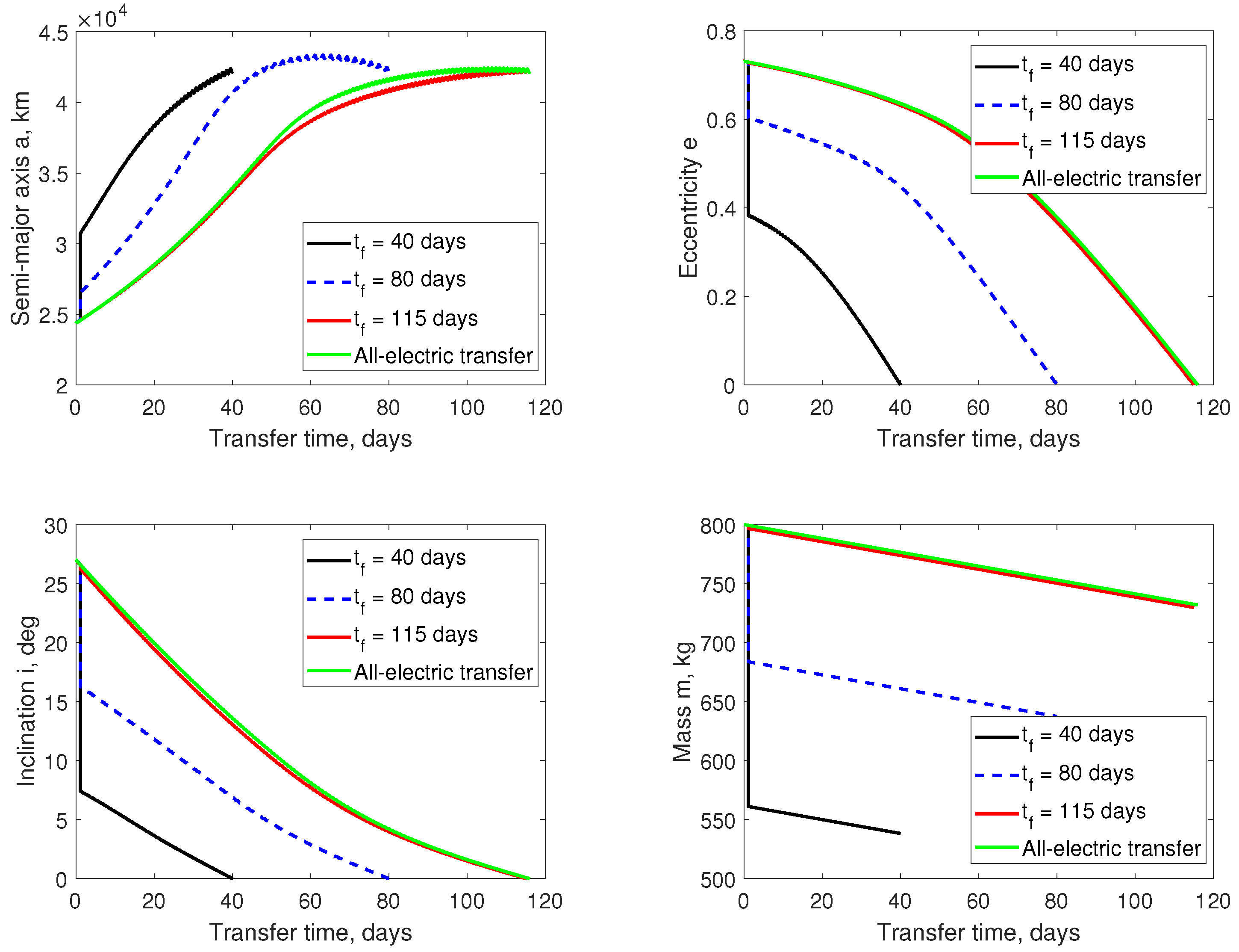
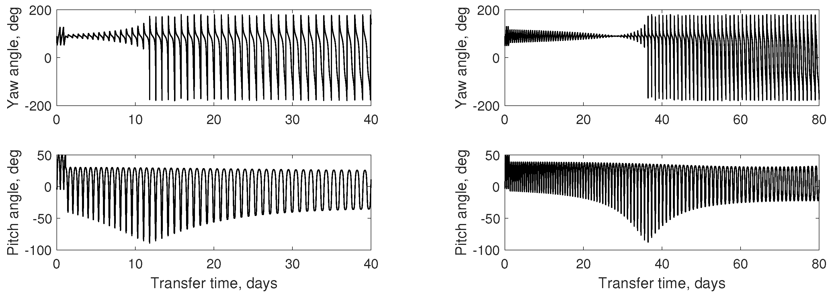
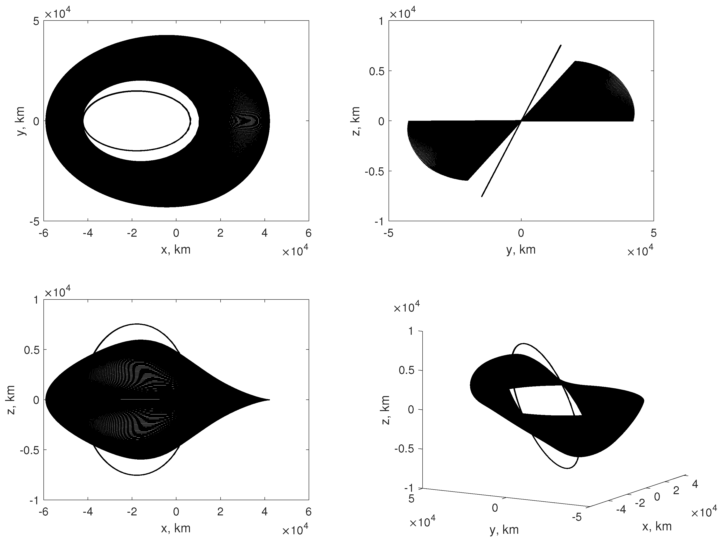
3.1. Solution of Hybrid Minimum-Fuel Hybrid Transfer

Firstly, hybrid transfer orbits with thrust magnitude $T_{\max }=200$ mN and low-thrust specific impulse $I_{sp}=3000$ s are optimized with various transfer times. MinPack-1 [30] and GNU Scientific Library (GSL) are used to solve the MPBVP. In this way, the convergence and efficiency of this algorithm can be discussed with different solvers. In GSL, the hybrid solver, discrete Newton solver and Broyden solver are considered to solve the MPBVP [31,32,33]. Moreover, the hybrid solver in GSL is based on MinPack. The computations are executed on a desktop personal computer with a CPU of 1.8 GHz, and Visual Studio 2019 is used. Considering the homotopic approach from $t_f^{\left(j\right)}$ to $t_f^{\left(j+1\right)}$, set $h_{t_f}=t_f^{\left(j+1\right)}-t_f^{\left(j\right)}$ days, and the maximum iteration number of the solvers in GSL is 100. When it does not converge, set $h_{t_f}=0.8h_{t_f}$. Part of the performance of the algorithm with the four solvers is listed in

Table 2. Performance of the algorithm with different solvers (computation time and fuel consumption of the solution).

${\mathit{t}}_{\mathit{f}}^{\left(\mathit{j}\right)}$(Days)	${\mathit{t}}_{\mathit{f}}^{\left(\mathit{j}+1\right)}$(Days)	MinPack-1	Hybrid	Discrete Newton	Broyden
40	42	1.8 s 257.22 kg	1.2 s 257.22 kg	4.7 s 257.22 kg	1.4 s 257.22 kg
70	72	4.9 s 182.28 kg	3.0 s 182.28 kg	8.6 s 182.28 kg	2.7 s 182.28 kg
100	105	6.9 s 96.59 kg	5.2 s 96.59 kg	19.5 s 96.59 kg	8.6 s 96.59 kg

. According to Table 2, this homotopic approach converges with all of the four solvers. The fuel consumption of the solution with four solvers is the same. However, the efficiency of solving this algorithm with MinPack-1, the hybrid solver and the Broyden solver in GSL is slightly higher than with the discrete Newton solver in GSL. Therefore, it is suggested to use Minpack-1, the hybrid solver and the Broyden solver in GSL to solve this problem. In the following works, MinPack-1 is used to solve this MPBVP.

In this case, chemical-only transfer orbit and all-electric transfer orbit are optimized first for comparison. The minimum time transfer problem with electric propulsion is solved by the indirect method [34] and thrust continuation. The fuel consumption of chemical-only transfer with two impulsive burns is $\mathsf{\Delta }{m}_c=366.86$ kg. Moreover, the magnitude of the two burns is, respectively, 1.805 km/s and 0.22 m/s. The minimum transfer time from GTO to GEO with all-electric propulsion is 115.942 days, and the fuel consumption is 68.10 kg.

For hybrid transfer with two impulsive burns with a transfer time of several days, the solution shows that the first impulsive burn is the same as that of hybrid transfer with one impulsive burn, and the magnitude of the second impulsive burn is 0. Moreover, the positions where the two impulsive burns are conducted are the same as those of chemical-only transfer. The first impulsive burn is conducted at the apogee to raise the perigee and lower the inclination, which is also the descending node. For GTO orbits, the apogee or the descending node is usually close to the GEO orbit (usually with an apogee of 42,164 km), which means that the delta-v of the second impulsive burn is almost 0 for chemical-only transfer. For hybrid transfer from GTO to GEO, the very small delta-v of the second impulsive burn can be completely replaced with the delta-v of EP in a short transfer time. As the magnitude of the second impulsive burn of hybrid transfer with two impulsive burns is 0, only hybrid transfer with one impulsive burn is considered for this transfer mission.

A series of hybrid transfer problems with transfer time varying from several days to 115 days are optimized. There are multiple local optimal solutions for the hybrid transfer problem. In the time continuation process, the timing of impulsive burn $t_1$ varies in a small range. When beginning from solutions with different $t_1$, the homotopy approach will lead to different solutions. In this work, two series of solutions with different values of $t_1$ are studied. The variation in fuel consumption $\mathsf{\Delta }m$ with transfer time $t_f$ and variation in the magnitude of impulsive burn $\mathsf{\Delta }{v}_1$ with $t_f$ are demonstrated in Figure 1. The timing of impulsive burn $t_1$ of the first series of solutions is 1.10 days, and $t_1$ of the second series of solutions is 0.66 days. According to Figure 1, when the transfer time is short enough, the hybrid transfer is close to chemical-only transfer, which requires fuel consumption of 366.86 kg. When the transfer time is close to the minimum transfer time with all-electric propulsion, the performance of hybrid transfer orbit is close to that of all-electric transfer orbit. The local optimal solutions with $t_1=1.10$ days perform better than those with $t_1=0.66$ days. Therefore, only solutions with $t_1=1.10$ days are discussed in the following section.

As is shown in Figure 1, there is a linear relation between fuel consumption $\mathsf{\Delta }m$ and transfer time $t_f$, and also an exponential relation between $\mathsf{\Delta }{v}_1$ and $t_f$. The curve-fitting result with $t_1=1.10$ days is presented in Figure 2. The curves are fitted with linear models, which hold the forms

$$exp\left(-\frac{\mathsf{\Delta }{v}_1}{I_{\mathrm{spc}}{g}_0}\right)=a_0+a_1{t}_f,$$

(38)

$$\mathsf{\Delta }m=b_0+b_1{t}_f$$

(39)

Combining Equations (12), (38) and (39), it can be derived that

$$\begin{array}{c}{b}_0=\left(m_0-\frac{T_{max}{t}_1}{I_{sp}{g}_0}\right)\left(1-a_0\right)\approx m_0\left(1-a_0\right),\\ b_1=-\left[a_1\left(m_0-\frac{T_{max}{t}_1}{I_{sp}{g}_0}\right)-\frac{T_{max}}{I_{sp}{g}_0}\right]\approx -\left(a_1{m}_0-\frac{T_{max}}{I_{sp}{g}_0}\right)\end{array}$$

(40)

Equation (40) describes the relation between coefficients $a_0$, $a_1$ and $b_0$, $b_1$. By MATLAB tool curve-fitting, the linear coefficients are solved:

$$\begin{array}{c}{a}_0=0.5441,a_1=3.9213\times {10}^{-3},\\ b_0=364.4245,b_1=-2.5471,\end{array}$$

(41)

where the units of $a_0$ and $a_1$ are, respectively, 1 and 1/day, and the units of $b_0$ and $b_1$ are, respectively, kg and kg/day. The goodness of the two models is guaranteed, with an $R^2$ statistical value of 0.9999. For a set of data $y_j$$\left(j=1,2,\dots ,n_y\right)$, the estimated value is ${\widehat{y}}_j$, and the average value is $\overline{y}$. The definition of $R^2$ is [35]

$$R^2=1-\frac{S}{S_{yy}},$$

(42)

where $S={\sum }_{j=1}^{n_y}{\left(y_j-{\widehat{y}}_j\right)}^2$ is the sum of the squares of the error, and $S_{yy}={\sum }_{j=1}^{n_y}{\left(y_j-\overline{y}\right)}^2$ is the total sum of squares. The root mean squared error (RMSE) is expressed as $\sqrt{{\sum }_{j=1}^{n_y}{\left(y_j-\widehat{y}\right)}^2/n_y}$. The value of $R^2$ lies between 0 and 1, where the value of 1 means a perfect fit. The curve-fitting result implies that when the transfer time is $t_f=0$, impulsive burn $\mathsf{\Delta }{v}_1$ and fuel consumption $\mathsf{\Delta }m$ satisfy that

$$\begin{array}{c}exp\left(-\frac{\mathsf{\Delta }{v}_1\left(0\right)}{I_{\mathrm{spc}}{g}_0}\right)=a_0=0.5441,\\ \mathsf{\Delta }m=b_0=364.42\mathrm{kg}\end{array}$$

(43)

Equation (43) means $\mathsf{\Delta }{v}_1=1.7906$ km/s and $\mathsf{\Delta }m=364.42$ kg, which is close to the performance of chemical-only transfer. When $\mathsf{\Delta }{v}_1=0$, it can be solved from the fitted linear model that $t_f=116.263$ days, which is close to the minimum time of all-electric transfer, $t_{EP}=115.942$ days. Theoretically, when $t_f$ reaches the minimum time of all-electric transfer, we have

$${\widehat{t}}_{EP}=t_f=\frac{1-a_0}{a_1}=\frac{1-exp\left(-\frac{\mathsf{\Delta }{v}_1\left(0\right)}{I_{\mathrm{spc}}{g}_0}\right)}{a_1}$$

(44)

where ${\widehat{t}}_{EP}$ represents the estimated minimum time of all-electric transfer. Because the value of ${\widehat{t}}_{EP}$ is independent of the term related to chemical propulsion, we have

$$a_1=\frac{1-exp\left(-\frac{\mathsf{\Delta }{v}_1\left(0\right)}{I_{\mathrm{spc}}{g}_0}\right)}{{\widehat{t}}_{EP}\left(T_{max},I_{sp}\right)}$$

(45)

Several previous investigations yielded the empirical conclusion that the product of low-thrust magnitude $T_{max}$ and minimum time of all-electric transfer $t_{EP}$ was nearly constant [6,28,36]. There is also a model suggested for the estimation of ${\widehat{t}}_{EP}$ [35,37]

$${\widehat{t}}_{EP}=c_1{\left(\frac{T_{max}}{m_0}\right)}^{d_1}{\left(I_{sp}\right)}^{d_3}+c_2{\left(\frac{T_{max}}{m_0}\right)}^{d_2}$$

(46)

The values of the coefficients vary with the initial and terminal orbits. However, for transfer missions from GTO to GEO and from LEO to GEO, the values of $d_1$ and $d_2$ are both near -1, which indicates that the empirical conclusion about the constancy of the product $t_{EP}\times T_{max}$ is practical in some cases. Combining Equations (44) and (46), we have the interpolation model in this work:

$$\frac{1-a_0}{a_1}=c_1{\left(\frac{T_{max}}{m_0}\right)}^{d_1}{\left(I_{sp}\right)}^{d_3}+c_2{\left(\frac{T_{max}}{m_0}\right)}^{d_2}$$

(47)

When the coefficients $c_1$, $c_2$, $d_1$, $d_2$ and $d_3$ are determined, the fuel consumption $\mathsf{\Delta }m$ and impulsive burn $\mathsf{\Delta }{v}_1$ can be estimated with transfer time $t_f$, low-thrust magnitude $T_{max}$, specific impulse of CP $I_{\mathrm{spc}}$ and specific impulse of EP $I_{sp}$.

The transportation rate $T_R$, which is the payload mass advantage gained by using EP divided by the low-thrust transit time [17], can be deduced from Equation (39):

$$T_R=\frac{\mathsf{\Delta }{m}_c-\mathsf{\Delta }m}{t_f}=\frac{\mathsf{\Delta }{m}_c-b_0}{t_f}-b_1$$

(48)

Because $\mathsf{\Delta }{m}_c-b_0$ = 2.44 kg, the first term on the right-hand side of Equation (48) can be neglected when $t_f$ is large enough, and the transportation rate is near constant $-b_1$. The actual transportation rate, deduced transportation rate in Equation (48) and simplified quadratic model are presented in Figure 3. For short-duration transfer with several days, the deduced model cannot be applied to estimate the transportation rate. This is because the error is enlarged when the term $\mathsf{\Delta }{m}_c-\mathsf{\Delta }m$ is divided by a small value of $t_f$. For hybrid transfer over 6 days, the deduced model is applicable for the estimation of the transportation rate.

Now, hybrid transfer orbits with transfer time of 40 days, 80 days and 115 days are shown among the transfer orbits with $t_1=1.10$ days. Moreover, the time-optimal transfer orbit with all-electric propulsion is also shown for comparison. The time histories of the semi-major axis, eccentricity, inclination and mass are presented in Figure 4. As is shown in Figure 4, the transfer orbit with $t_f=115$ days is close to the all-electric transfer orbit. For hybrid transfer orbits with transfer time of 40 days and 80 days, time histories of thrust direction angles in the RSW reference frame are illustrated in Figure 5. The trends of thrust direction and the transfer orbit with transfer time of 80 days are shown in Figure 6. As is presented in Figure 6, the impulsive burn is conducted at the ascending/descending node, which is also the apogee, to raise the perigee and lower the inclination.

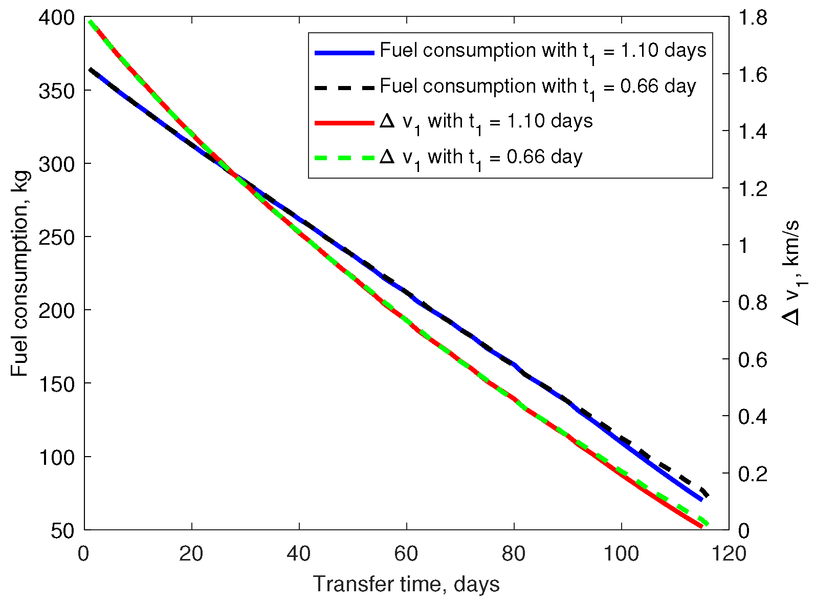
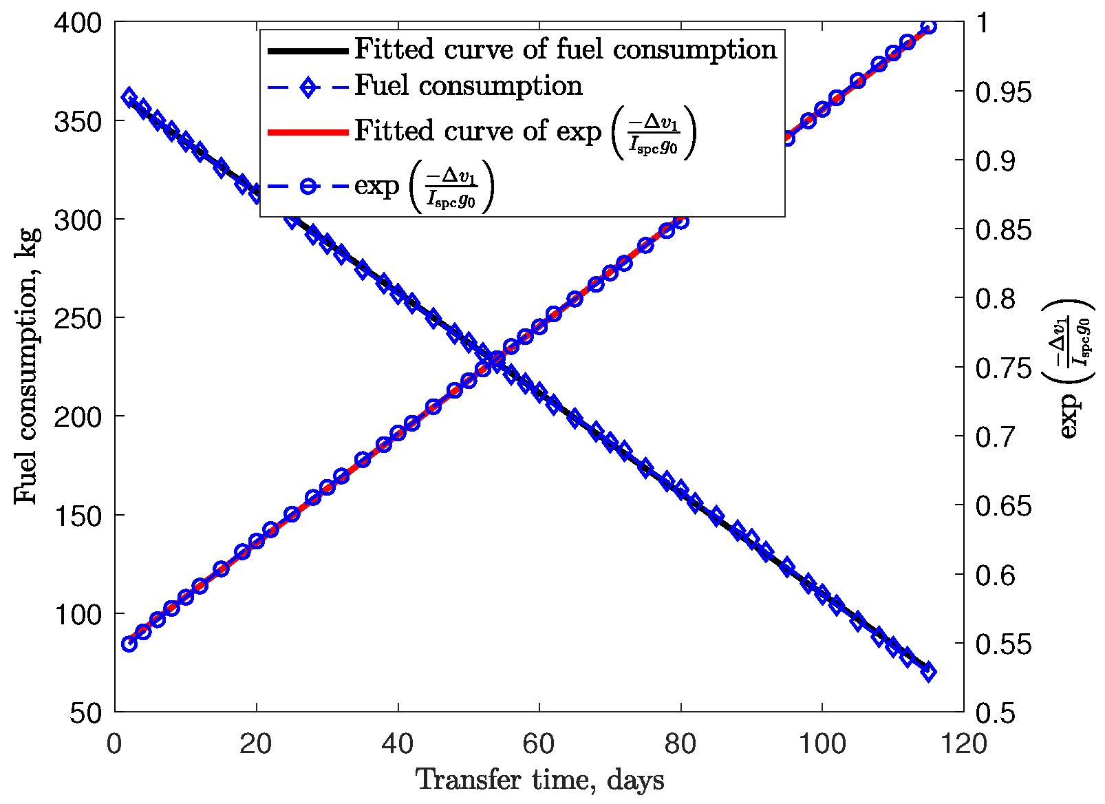
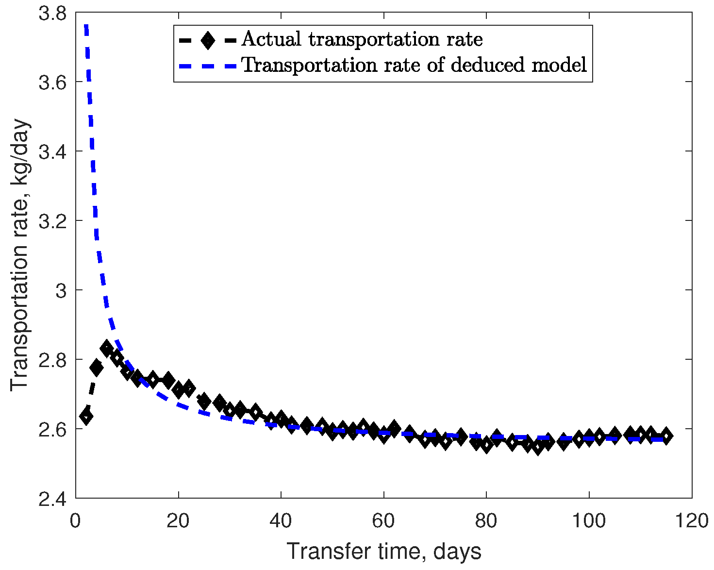
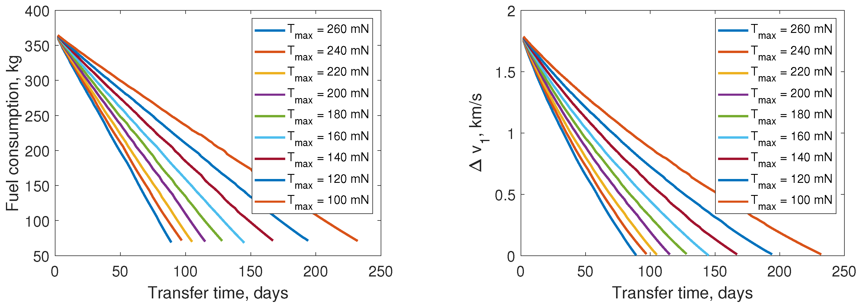
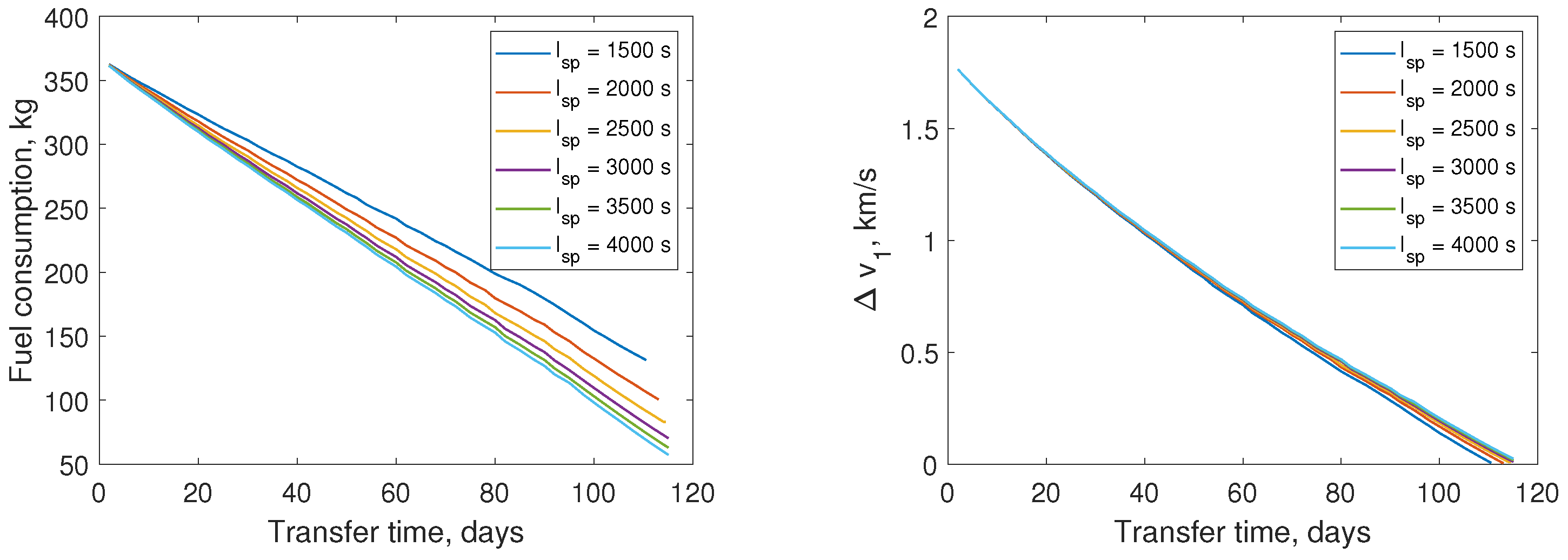
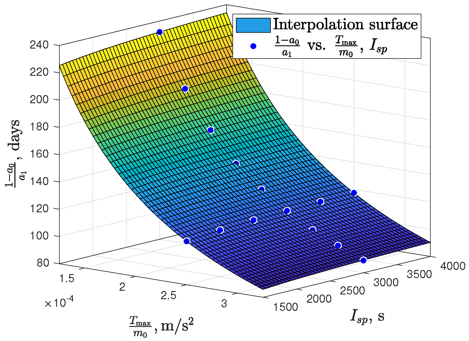
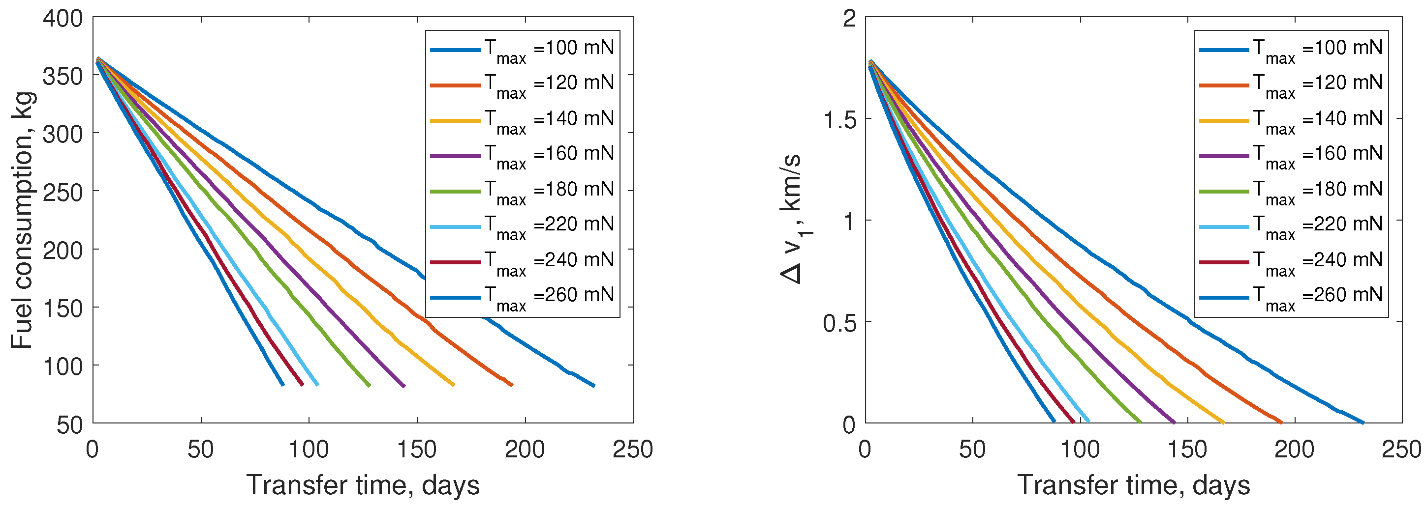
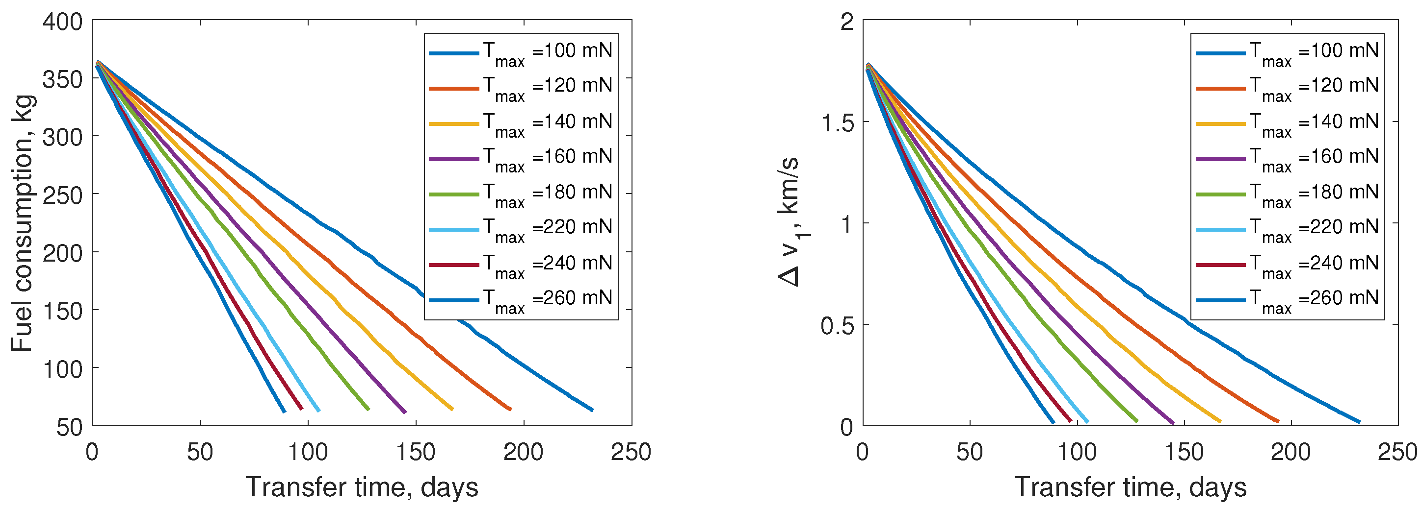
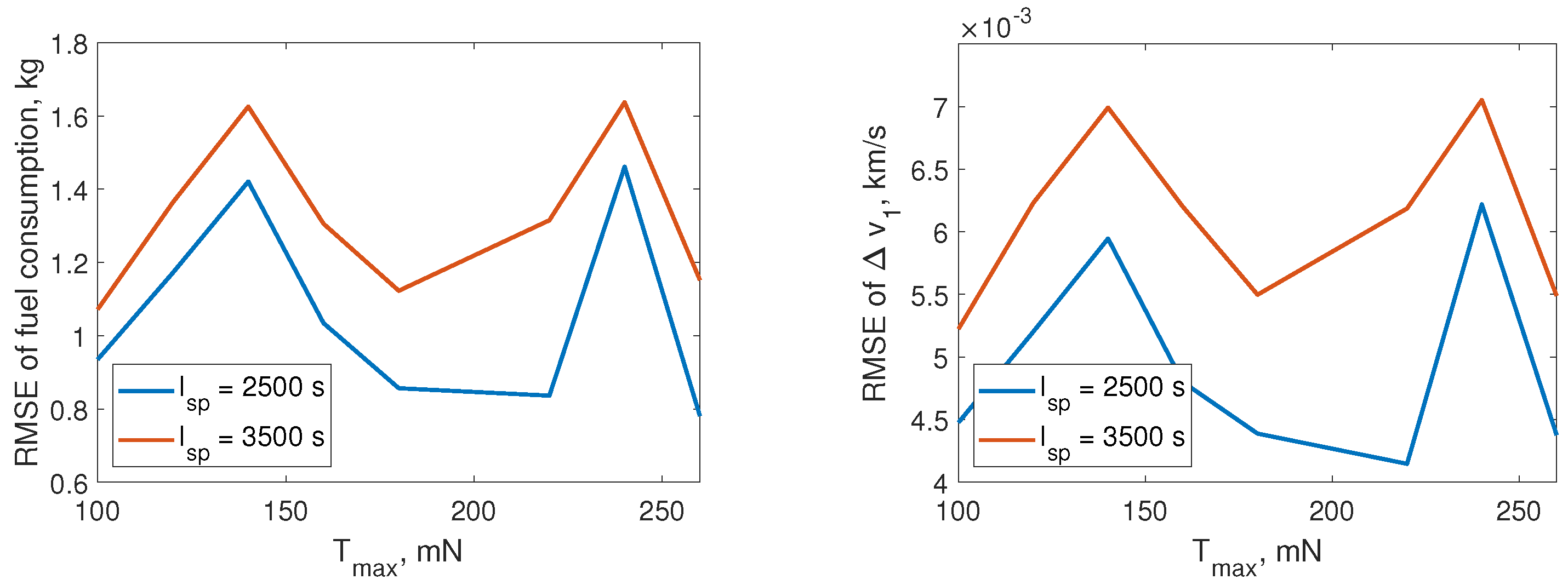
3.2. Performance of Hybrid Transfer with Various Low-Thrust Maximum Magnitude and Specific Impulse

As is mentioned above, the linear coefficients in Equations (38) and (39) are related to low-thrust maximum magnitude $T_{max}$ and specific impulse $I_{sp}$. A group of values of $T_{max}$ and $I_{sp}$ are considered to determine the coefficients in Equation (46). The hybrid transfer problems are solved when $T_{max}$ and $I_{sp}$ are set with different values. When $T_{max}$ takes various values, the variation in fuel consumption $\mathsf{\Delta }m$ with transfer time $t_f$ and the variation in the magnitude of the impulsive burn $\mathsf{\Delta }{v}_1$ with $t_f$ are demonstrated in Figure 7. When $I_{sp}$ takes various values, the variation in fuel consumption $\mathsf{\Delta }m$ with transfer time $t_f$ and the variation in the magnitude of impulsive burn $\mathsf{\Delta }{v}_1$ with $t_f$ are demonstrated in Figure 8. The data are fitted with the linear model presented in Equations (38) and (39). Then, the coefficients $a_0$ and $a_1$ can be obtained on different occasions.

With the model described in Equation (47) for curve fitting, the coefficients of the interpolation model are shown in

Table 3. Coefficients of the interpolation model.

${\mathit{c}}_1$	${\mathit{c}}_2$	${\mathit{d}}_1$	${\mathit{d}}_2$	${\mathit{d}}_3$
−3.99577	0.03540	−0.70065	−0.98333	−0.65100

. The goodness of the fit is guaranteed, with an $R^2$ statistical value of 1.0000. The interpolation surface is illustrated in Figure 9. In these cases, the coefficient $a_0$ varies between 0.5413 and 0.5453, and its average value is 0.5441. Therefore, the coefficient $a_0$ is determined as $a_0=0.5441$. Then, the coefficient $a_1$ can be obtained using Equation (47), and coefficients $b_0$ and $b_1$ can be computed with Equation (40).

The value of the term $c_1{\left(\frac{T_{max}}{m_0}\right)}^{d_1}{\left(I_{sp}\right)}^{d_3}$ is much smaller than that of the term $c_2{\left(\frac{T_{max}}{m_0}\right)}^{d_2}$ in Equation (47). Moreover, the value of $d_2$ is 0.98333, which is close to −1. This suggests that the product $\left(1-a_0\right)/a_1\times T_{max}$ is nearly constant when $I_{sp}$ is fixed, which has only a small range of variation. This simplified conclusion can be applied for a fast estimation of $a_1$ with low precision.

Once the coefficients are determined, the model can be applied for estimating the fuel consumption $\mathsf{\Delta }m$ and impulsive burn $\mathsf{\Delta }{v}_1$. The hybrid transfer problems with another group of values of $T_{max}$ and $I_{sp}$ are solved for validation. When $I_{sp}=2500$ s and $I_{sp}=3500$ s, considering different values of $T_{max}$, the variation in fuel consumption $\mathsf{\Delta }m$ with transfer time $t_f$, and the variation in the magnitude of impulsive burn $\mathsf{\Delta }{v}_1$ with $t_f$ are, respectively, illustrated in Figure 10 and Figure 11. The values of RMSE of the model for estimation are presented in Figure 12. Applying this model for estimation, the RMSE of the fuel consumption is no more than 2 kg, and the RMSE of the magnitude of impulsive burn is approximately ${10}^{-3}$ km/s.

Among these cases, the case where $T_{max}=100$ mN, $I_{sp}=3500$ s is discussed as an example. The variation in relative error $\left(\mathsf{\Delta }\widehat{m}-\mathsf{\Delta }m\right)/\mathsf{\Delta }m$ with transfer time $t_f$ and the variation in error $\mathsf{\Delta }{\widehat{v}}_1-\mathsf{\Delta }{v}_1$ with transfer time $t_f$ are presented in Figure 13. It can be seen that the estimated fuel consumption error is less than 5%, and the estimated error of the impulsive burn’s magnitude is within 0.015 km/s. The estimation of the transportation rate is shown in Figure 14. Starting from $t_f=10$ days, the estimated transportation rates are essentially the same as the real transportation rates. The large error with a small value of $t_f$ has been explained before. The relative error of the transportation rate is presented in Figure 15, where the error with $t_f$ less than 10 days is ignored. It can be seen from Figure 15 that the transportation error is mainly within 2%.

4. Discussion and Conclusions

In this paper, a trajectory optimization method is proposed for time-fixed minimum-fuel orbital transfer with combined chemical–electric propulsion. The first-order necessary conditions for impulsive burn constraints are derived analytically. The long-duration geostationary orbit transfer is many-revolution, and is solved through the homotopic approach from the short-duration transfer problem. For hybrid transfer missions from GTO to GEO, the solution of hybrid transfer with two impulsive burns shows that the magnitude of the second impulsive burn is 0, which indicates that only hybrid transfer with one impulsive burn should be considered.

There are multiple local optimal solutions of this problem. Some of the local optimal solutions have different timings of impulsive burn $t_1$. When the transfer time is close to 0, the performance of hybrid transfer is close to that of chemical-only transfer. Moreover, when the transfer time reaches the minimum all-electric transfer time, the performance of the hybrid transfer is close to that of all-electric transfer. The variation in fuel consumption with transfer time is nearly linear, and the variation in the magnitude of the impulsive burn is exponential. The models in Equations (38) and (39) are applied to describe the two relations. According to the linear coefficients $a_0$ and $b_0$, the magnitude of impulsive burn $\mathsf{\Delta }{v}_1$ and fuel consumption at $t_f=0$ are close to those of chemical-only transfer. The coefficients $a_0$ and $b_0$ are constant when the specific impulse of chemical propulsion $I_{\mathrm{spc}}$ is fixed. The coefficient $a_1$ can be expressed with $a_0$ and the estimated minimum time of all-electric transfer ${\widehat{t}}_{EP}$. The value of ${\widehat{t}}_{EP}$ is estimated with an interpolation model. The coefficients of the interpolation model are related to the initial and terminal orbits. Once the coefficients are determined, the model can be applied for estimating the fuel consumption and magnitude of the impulsive burn with a given transfer time, specific impulse of the propulsion system and low-thrust magnitude. A group of hybrid transfer cases with various low-thrust magnitude $T_{max}$ and specific impulse of EP $I_{sp}$ are optimized to offer data for the determination of the coefficients. Then, a new group of hybrid transfer cases are optimized for the validation of the model. The initial mass of the spacecraft is 800 kg, and the specific impulse of CP is fixed with $I_{\mathrm{spc}}=300$ s. For the cases for validation, the RMSE of the fuel consumption is within 2 kg, and the RMSE of magnitude of the impulsive burn is approximately ${10}^{-3}$ km/s. For hybrid transfer with $T_{max}=100$ mN and $I_{sp}=3500$ s, the fuel consumption prediction error is less than 5%. The error of the impulsive burn’s magnitude is within 0.015 km/s. Finally, the transportation error is mainly within 2%.

Because this paper is based on some assumptions, the solution of this method is not accurate enough to design a precise transfer trajectory. The results and model can be used to provide an initial solution for existing software or programs such as GMAT, which can be used to further design a precise transfer trajectory.

References

1. Martinez-Sanchez, M.; Pollard, J.E. Spacecraft electric propulsion-an overview. J. Propuls. Power 1998, 14, 688–699. [Google Scholar] [CrossRef] [Green Version]
2. Yang, G. Direct optimization of low-thrust many-revolution earth-orbit transfers. Chin. J. Aeronaut. 2009, 22, 426–433. [Google Scholar] [CrossRef] [Green Version]
3. Scheel, W.A.; Conway, B.A. Optimization of very-low-thrust, many-revolution spacecraft trajectories. J. Guid. Control Dyn. 1994, 17, 1185–1192. [Google Scholar] [CrossRef]
4. Dalin, Y.; Bo, X.; Youtao, G. Optimal strategy for low-thrust spiral trajectories using Lyapunov-based guidance. Adv. Space Res. 2015, 56, 865–878. [Google Scholar] [CrossRef]
5. Hargraves, C.R.; Paris, S.W. Direct Trajectory Optimization Using Nonlinear Programming and Collocation. J. Guid. Control Dyn. 1987, 10, 338–342. [Google Scholar] [CrossRef]
6. Haberkorn, T.; Martinon, P.; Gergaud, J. Low thrust minimum-fuel orbital transfer: A homotopic approach. J. Guid. Control Dyn. 2004, 27, 1046–1060. [Google Scholar] [CrossRef] [Green Version]
7. Quarta, A.A.; Mengali, G.; Bassetto, M. Optimal solar sail transfers to circular Earth-synchronous displaced orbits. Astrodynamics 2020, 4, 193–204. [Google Scholar] [CrossRef]
8. Gao, Y.; Kluever, C. Low-Thrust Interplanetary Orbit Transfers Using Hybrid Trajectory Optimization Method with Multiple Shooting. In Proceedings of the AIAA/AAS Astrodynamics Specialist Conference and Exhibit, Providence, RI, USA, 16–19 August 2004; Volume 2. [Google Scholar] [CrossRef]
9. Ilgen, M.R. A hybrid method for computing optimal low thrust otv trajectories. Spacefl. Mech. 1994, 2, 941–958. [Google Scholar]
10. Petropoulos, A.E. Simple Control Laws for Low-Thrust Orbit Transfers; Jet Propulsion Laboratory, National Aeronautics and Space Administration: Pasadena, CA, USA, 2003. [Google Scholar]
11. Ilgen, M.R. Low thrust OTV guidance using Liapunov optimal feedback control techniques. Astrodynamics 1994, 85, 1527–1545. [Google Scholar]
12. Bassetto, M.; Quarta, A.A.; Mengali, G.; Cipolla, V. Spiral trajectories induced by radial thrust with applications to generalized sails. Astrodynamics 2021, 5, 121–137. [Google Scholar] [CrossRef]
13. Feuerborn, S.A.; Perkins, J.; Neary, D.A. Finding a way: Boeing’s all electric propulsion satellite. In Proceedings of the 49th AIAA/ASME/SAE/ASEE Joint PropulsionConference, San Jose, CA, USA, 15–17 July 2013; p. 4126. [Google Scholar]
14. Rovey, J.L.; Lyne, C.T.; Mundahl, A.J.; Rasmont, N.; Glascock, M.S.; Wainwright, M.J.; Berg, S.P. Review of multimode space propulsion. Prog. Aerosp. Sci. 2020, 118, 100627. [Google Scholar] [CrossRef]
15. Oleson, S.R.; Myers, R.M.; Kluever, C.A.; Riehl, J.P.; Curran, F.M. Advanced propulsion for geostationary orbit insertion and north-south station keeping. J. Spacecr. Rocket. 1997, 34, 22–28. [Google Scholar] [CrossRef] [Green Version]
16. Mailhe, L.M.; Heister, S.D. Design of a hybrid chemical/electric propulsion orbital transfer vehicle. J. Spacecr. Rocket. 2002, 39, 131–139. [Google Scholar] [CrossRef]
17. Oh, D.Y.; Randolph, T.; Kimbrel, S.; Martinez-Sanchez, M. End-to-end optimization of chemical-electric orbit-raising missions. J. Spacecr. Rocket. 2004, 41, 831–839. [Google Scholar] [CrossRef]
18. Jenkin, A. Representative mission trade studies for low-thrust transfers to geosynchronous orbit. In Proceedings of the AIAA/AAS Astrodynamics Specialist Conference and Exhibit, Honolulu, HI, USA, 18–21 August 2004; p. 5086. [Google Scholar]
19. Kluever, C.A. Optimal geostationary orbit transfers using onboard chemical-electric propulsion. J. Spacecr. Rocket. 2012, 49, 1174–1182. [Google Scholar] [CrossRef]
20. Kluever, C.A. Designing transfers to geostationary orbit using combined Chemical–Electric propulsion. J. Spacecr. Rocket. 2015, 52, 1144–1151. [Google Scholar] [CrossRef]
21. Morante, D.; Sanjurjo Rivo, M.; Soler, M. A survey on low-thrust trajectory optimization approaches. Aerospace 2021, 8, 88. [Google Scholar] [CrossRef]
22. Hughes, S.P.; Qureshi, R.H.; Cooley, S.D.; Parker, J.J. Verification and validation of the general mission analysis tool (GMAT). In Proceedings of the AIAA/AAS Astrodynamics Specialist Conference, San Diego, CA, USA, 4–7 August 2014; p. 4151. [Google Scholar]
23. Sauer, J.R.C. Optimization of multiple target electric propulsion trajectories. In Proceedings of the 11th Aerospace Sciences Meeting, Washington, DC, USA, 10–12 January 1973; p. 205. [Google Scholar]
24. Walker, M.; Ireland, B.; Owens, J. A set modified equinoctial orbit elements. Celest. Mech. 1985, 36, 409–419. [Google Scholar] [CrossRef]
25. Bryson, A.E. Applied Optimal Control: Optimization, Estimation and Control; CRC Press: Boca Raton, FL, USA, 1975. [Google Scholar]
26. Fehlberg, E. Classical fifth-, sixth-, seventh-, and eighth-order Runge-Kutta formulas with stepsize Control. NASA Tech. Rep. 1968, R-287. [Google Scholar]
27. Lei, H.; Xu, B.; Sun, Y. Earth–Moon low energy trajectory optimization in the real system. Adv. Space Res. 2013, 51, 917–929. [Google Scholar] [CrossRef]
28. Caillau, J.B.; Gergaud, J.; Noailles, J. 3D geosynchronous transfer of a satellite: Continuation on the thrust. J. Optim. Theory Appl. 2003, 118, 541–565. [Google Scholar] [CrossRef]
29. Pan, B.; Lu, P.; Pan, X.; Ma, Y. Double-homotopy method for solving optimal control problems. J. Guid. Control Dyn. 2016, 39, 1706–1720. [Google Scholar] [CrossRef]
30. Moré, J.J.; Garbow, B.S.; Hillstrom, K.E. User Guide for MINPACK-1; Technical Report, CM-P00068642; Cern Libraries: Geneva, Italy, 1980. [Google Scholar]
31. Powell, M.J. A hybrid method for nonlinear equations. In Numerical Methods for Nonlinear Algebraic Equations; Gordon and Breach: London, UK, 1970. [Google Scholar]
32. Moré, J.J.; Cosnard, M.Y. Numerical solution of nonlinear equations. ACM Trans. Math. Softw. (TOMS) 1979, 5, 64–85. [Google Scholar] [CrossRef]
33. Broyden, C.G. A class of methods for solving nonlinear simultaneous equations. Math. Comput. 1965, 19, 577–593. [Google Scholar] [CrossRef]
34. Li, H.; Baoyin, H.; Topputo, F. Neural Networks in Time-Optimal Low-Thrust Interplanetary Transfers. IEEE Access 2019, 7, 156413–156419. [Google Scholar] [CrossRef]
35. Graham, K.F.; Rao, A.V. Minimum-time trajectory optimization of multiple revolution low-thrust earth-orbit transfers. J. Spacecr. Rocket. 2015, 52, 711–727. [Google Scholar] [CrossRef] [Green Version]
36. Yue, X.; Yang, Y.; Geng, Z. Indirect optimization for finite-thrust time-optimal orbital maneuver. J. Guid. Control Dyn. 2010, 33, 628–634. [Google Scholar] [CrossRef]
37. Ramos Moron, N. Indirect Optimization of Electric Propulsion Orbit Raising to GEO with Homotopy. Master’s Thesis, Politecnico di Milano—School of Industrial and Information Engineering, Milan, Italy, 27 July 2017. [Google Scholar]
Figure 1. The variation in fuel consumption with transfer time and variation in magnitude of impulsive burn with transfer time.
Aerospace 09 00200 g001
Figure 2. Curve-fitting results of fuel consumption and impulsive burn’s magnitude.
Aerospace 09 00200 g002
Figure 3. Transportation rate versus transfer time.
Aerospace 09 00200 g003
Figure 4. The time histories of the semi-major axis, eccentricity, inclination and mass of hybrid transfer orbit with transfer time of 40 days, 80 days, 115 days and all-electric transfer orbit.
Aerospace 09 00200 g004
Figure 5. The time histories of thrust direction angles with transfer time of 40 days and 80 days.
Aerospace 09 00200 g005
Figure 6. Hybrid transfer orbit when transfer time is 80 days.
Aerospace 09 00200 g006
Figure 7. The variation in fuel consumption with transfer time and variation in magnitude of impulsive burn with transfer time for different values of T max when I s p = 3000 s.
Aerospace 09 00200 g007
Figure 8. The variation in fuel consumption with transfer time and variation in magnitude of impulsive burn with transfer time for different values of I s p when T max = 200 mN.
Aerospace 09 00200 g008
Figure 9. Interpolation surface and the real values of 1 a 0 / a 1 .
Aerospace 09 00200 g009
Figure 10. The variation in fuel consumption with transfer time and variation in magnitude of impulsive burn with transfer time for different values of T max when I s p = 2500 s.
Aerospace 09 00200 g010
Figure 11. The variation in fuel consumption with transfer time and variation in magnitude of impulsive burn with transfer time for different values of T max when I s p = 3500 s.
Aerospace 09 00200 g011
Figure 12. RMSE of the estimation of fuel consumption and magnitude of impulsive burn with the interpolation model.
Aerospace 09 00200 g012
Figure 13. Prediction error of fuel consumption and magnitude of impulsive burn when T max = 100 mN and I s p = 3500 s.
Aerospace 09 00200 g013
Figure 14. Transportation rate versus transfer time when T max = 100 mN and I s p = 3500 s.
Aerospace 09 00200 g014
Figure 15. Transportation rate error versus transfer time when T max = 100 mN and I s p = 3500 s.
Aerospace 09 00200 g015