Article

Active Fault-Tolerant Control for Near-Space Hypersonic Vehicles

1
School of Astronautics, Beihang University (BUAA), Beijing 100191, China
2
School of Automation Science and Electrical Engineering, Beihang University (BUAA), Beijing 100191, China
*
Author to whom correspondence should be addressed.
Aerospace 2022, 9(5), 237; https://doi.org/10.3390/aerospace9050237
Submission received: 12 March 2022 / Revised: 19 April 2022 / Accepted: 22 April 2022 / Published: 25 April 2022
(This article belongs to the Special Issue AI/Machine Learning in Aerospace Autonomy)

Abstract

:
Due to the harsh working environment, Near-Space Hypersonic Vehicles (NSHVs) have the characteristics of frequent faults, which seriously affect flight safety. However, most researches focus on active fault-tolerant control for actuator faults. In order to fill the gap of active fault-tolerant control for sensor faults, this paper presents an Active Fault-Tolerant Control (AFTC) strategy for NSHVs based on Active Disturbance Rejection Control (ADRC) combined with fault diagnosis and evaluation. With the proposed AFTC strategy, both sensor faults and actuator faults can be compensated within 0.5 s. Wavelet packet decomposition and Kernel Extreme Learning Machine (KELM) are associated to ensure the high accuracy and real-time ability of fault diagnosis. Simulation results show that the proposed fault diagnosis method can significantly reduce the divergence of diagnosis results by up to 98%. The fault information is used to generate tolerant compensation, which is combined with the ADRC to achieve AFTC. Statistical results indicate that AFTC has significantly lower static error than ADRC. The proposed AFTC method endows NSHVs with the ability to complete missions even when various types of faults appear. Its advantages are demonstrated in comparison with other fault diagnosis and tolerant control methods.

1. Introduction

In recent years, Near-Space Hypersonic Vehicles (NSHVs) have become the central issue in aerospace. However, due to the severe near-space flight environment, NSHVs are prone to various types of small faults with concurrency [1,2]. Moreover, in the dynamic closed-loop system, small faults are easily amplified into significant faults, leading to serious consequences. The existence of the closed-loop control strategy causes fault deterioration, which can mask early features [3]. Therefore, the design of a high-quality fault-tolerant control strategy is urgently needed and becomes a new hotspot [4,5].
Fault-tolerant control methods for complex nonlinear systems are divided into Passive Fault-Tolerant Control (PFTC) and Active Fault-Tolerant Control (AFTC) [6]. A PFTC system is designed by experts, which can accommodate prescribed faults using its robustness, without the knowledge of faults [7,8]. Active Disturbance Rejection Control (ADRC) is widely used in PFTC for its simple structure and outstanding performance in anti-disturbance and actuator fault tolerance. Zhang et al. [9] designed a double closed-loop ADRC for the quadrotor UAV, and the total disturbances are estimated and compensated by ESO which can improve the anti-disturbance ability.
On the contrary, an AFTC strategy requires the fault information to reconstruct the controller. The fault information is provided by an onboard fault diagnosis and evaluation unit. Compared with PFTC, the addition of fault information makes AFTC more adaptable, and makes it possible to solve sensor faults. And that’s why AFTC has become a new research focus [5,10,11,12]. Xu et al. [13] developed an adaptive fault-tolerant control method for hypersonic vehicles considering unexpected elevator faults, uncertain parameters, and external disturbances. Wu et al. [14] used a fault diagnosis unit, based on the long short-term memory neural network, to diagnose actuator faults, and the fault tolerance was realized both in the control allocation and control layers. However, the papers above focus on the actuator faults, but neglect fault tolerance for sensor faults. For the severe flight environment, actuator faults and sensor faults are common for NSHVs. Therefore, both of these faults are considered in this paper.
For NSHVs, both PFTC and AFTC have been widely studied. The former needs the system to be strong enough in face of faults, but cannot well handle significant faults. The latter has higher fault tolerance ability for obvious faults. However, study on the AFTC concentrates mainly on actuator faults, relying on the correct sensors’ feedback. Table 1 shows the capabilities of different control methods. It’s evident that sensor faults should also be taken into consideration for AFTC [15,16,17].
An AFTC system usually consists of three parts: a PFTC unit, a fault diagnosis and evaluation unit, and a controller reconstruction unit [18,19]. The use of PFTC is to track the control instruction and implement passive fault tolerance before the controller is reconstructed when there are faults. The key point of fault diagnosis and evaluation unit is to get information about faults. To some extent, the accuracy of fault diagnosis and evaluation decides the effect of AFTC. Thus, different methods have been researched explosively. Currently, the widely used methods are mainly divided into two categories, namely model-based methods and data-driven methods [20]. Model-based methods rely on the mathematical of models, which are unsuitable for complex nonlinear systems such as NSHVs. Meanwhile, in data-driven methods, machine-learning methods are generally used, such as neural networks or classifiers. The advantage is that accurate models are not required, which are more beneficial for complex systems [21]. To achieve AFTC, the fault diagnosis and evaluation unit should gives types and severity of faults to the subsequent controller. Meanwhile, it should have the capability of real-time computing. Considering noises and various types of faults, higher requirements are put forward for fault diagnosis.
Above all, although plenty of researches have focused on Fault Tolerant Control (FTC) or fault diagnosis, there are still some problems that need to be solved: (1) most of the PFTC-adopted researches are helpful for actuator faults depending on the correct sensors’ feedback, but cannot handle sensor faults [17,22,23]; (2) plenty of researchers focus on faults classification, ignoring the requirement of faults identification [24,25]. Motivated by the aforementioned challenges and demands, this paper proposes a novel Active Disturbance Rejection Control and Kernel Extreme Learning Machine (ADRC-KELM) based AFTC scheme for NSHVs with actuator faults and sensor faults.
The main contribution of this paper is to introduce a novel method for fault diagnosis, evaluation and AFTC algorithm for NSHVs. The introduction of sliding window and KELM enables faults diagnosis less than 0.5 s. Furthermore, the joint time-frequency analysis makes fault identification possible. Finally, the AFTC endows NSHVs with the ability to complete missions in the face of multiple faults.
The remainder of this paper is organized as follows. In Section 2, model of NSHVs, the Reaction Control System (RCS), and an ADRC controller are proposed. Details of ADRC-KELM based AFTC are addressed in Section 3. In Section 4, results of various simulations are illustrated and analyzed. Finally, Section 5 draws the conclusion.

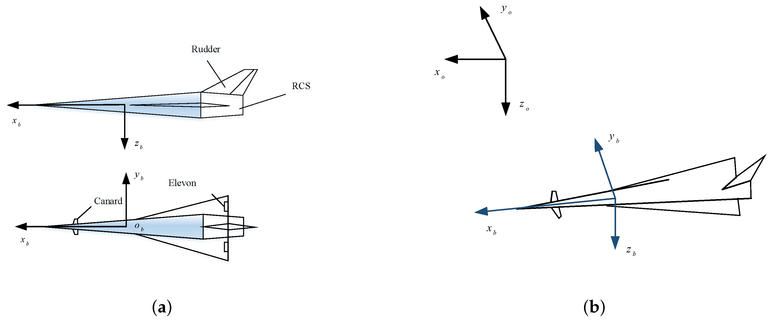
2. Nonlinear Model of NSHV with Closed-Loop Faults

In this section, a nonlinear model is provided. The nonlinear model established under ideal conditions lays the foundation for flight simulation experiments. The PFTC is established for disturbance rejection and uncertainty suppression. Main ideas and implementation of the AFTC method are briefly described in Figure 1.
The AFTC method is composed of two parts: online and offline. The task of the offline part is to train KELM for obtaining an efficient classifier. First, simulation results of different states constitute the database. Then Wavelet Packet Transformation (WPT) is used to extract features to train the KELM. For the online part, a sliding window is adopted to realize real-time fault diagnosis. And the trained parameters are passed to classify faults. Finally, joint time-frequency analysis of the residual signal is employed to identify fault sizes.
As shown in Figure 2a, the studied NSHV has delta wings, foldable horizontal canards, a vertical tail, and the RCS. Due to the low atmospheric density, the aerodynamic rudder surface efficiency is insufficient, which makes it difficult to meet the control requirements. Therefore, RCS is adopted to complete attitude control.
Figure 2b depicts the inertia coordinate o x o y o z o , body coordinate o x b y b z b . Without loss of generality, only the longitudinal channel of the aircraft is considered. The reentry process of the NSHV can be modeled by the following equations:
x ˙ = v cos γ z ˙ = v sin γ v ˙ = ( D m g sin γ T y sin α ) m γ ˙ = Y + T y cos α m g cos γ m v α ˙ = ω y γ ˙ ω ˙ = l T y I y y ,
where x , z denote the position of the NSHV in the inertia coordinate system. v is the velocity. γ , α denote the trajectory inclination angle and the angle of attack, respectively. m is the mass of NSHV, which is regarded as a constant. g indicates the gravitational acceleration. D , T y , Y are the aerodynamic drag, propulsion, and aerodynamic force, respectively. w y represents the pitch angular rate. I y denotes the moment of inertia for the y coordinate axes. l means the distance from the RCS to the center of mass. More details are cited from [1].

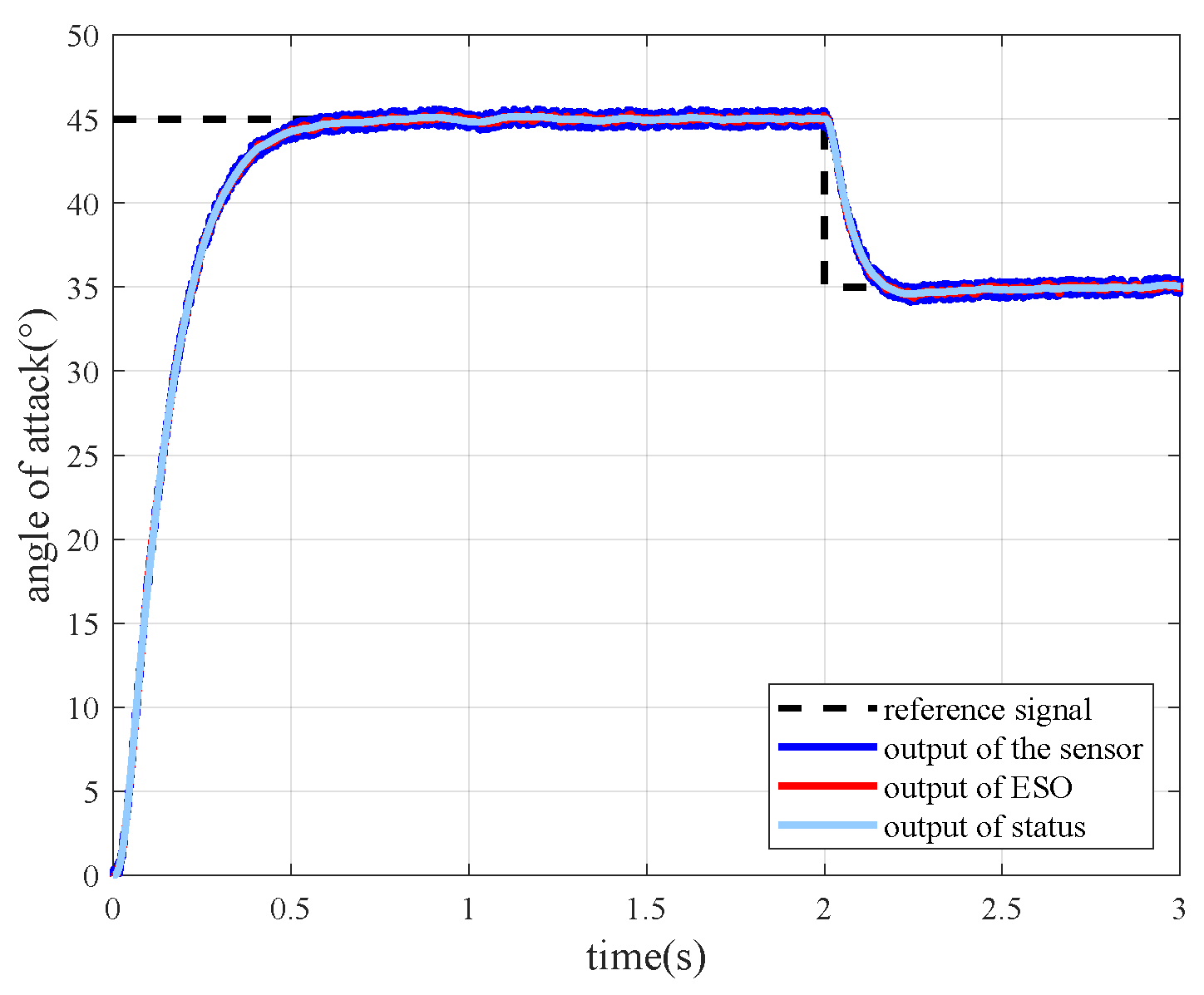
2.1. NSHV Passive Fault-Tolerant Control

The construction of ADRC is designed as Figure 3. The Extended State Observer (ESO) can be regarded as a reference model, which is established as follow:
e = z 1 θ z ˙ 1 = z 2 β 1 e z ˙ 2 = z 3 β 2 e + b u z ˙ 3 = β 3 e ,
where z 1 , z 2 , z 3 are observations of ESO, which are angle of attack, its differential, and the total disturbance. e is the residual signal. β 1 , β 2 , β 3 are the tunable parameters with different values, which are generally determined by the bandwidth of the observer and can affect tracking performance [26]. The Tracking Differentiator (TD) is defined as follows:
a 1 ( k + 1 ) = a 1 ( k ) + T s a 2 ( k ) a 2 ( k + 1 ) = a 2 ( k ) T s ( ( a 1 ( k ) T c 2 a * ( k ) ) + 2 a 2 ( k ) T c ) ,
where a 1 ( k ) , a 1 ( k + 1 ) denote the estimated angle values of the current time and next time, respectively. a 2 ( k ) , a 2 ( k + 1 ) are the derivatives of a 1 ( k ) , a 1 ( k + 1 ) , respectively. a * ( k ) represents the desired signal. T s and T c are the sampling time and the time constant, respectively. The larger T s , the better noise filtering [27].

2.2. Description and Modeling of Actuator Faults and Sensor Faults

During the stage of reentry, for the low atmospheric density, RCS is necessary for attitude control. Actuators directly decide the performance of control. That’s why FTC for actuators is widely studied. But for sensor faults, most researchers regard them as interference terms and their causes are ignored. Building on previous work, the fault mechanisms are summarized [3,28,29].
Stuck fault: The output maintains a certain value and no longer changes. For RCS, once the adjust venturi tubes are stuck, the thrust maintains a constant value. For sensors, it is usually caused by unstable signal transmission.
Gain variation fault: The output deviates from the desired value. Usually, gain is multiplied by the desired value. For RCS, this fault is mainly caused by the change of throat diameter due to ablation. For sensors, temperature change and parts aging usually cause a slight variation or static error.
Outlier data fault: This kind of fault is a short-term fault. When it occurs, the output changes suddenly and returns to normal quickly without lasting effect, which is unique for sensor faults. This occurs when there is communication interference or other disturbances.
Above all, the faults are summarized as follows:
O f , s = O ( t ) + f a l s ( O ( t ) , t s ) O f , g = O ( t ) + f a l g ( O ( t ) , K g , t g ) O f , o = O ( t ) + f a l o ( O ( t ) , δ , t o ) ,
where O ( t ) is the output of sensors or actuators. O f , s , O f , g , O f , o are outputs under the stuck fault, the gain variation fault, and the outlier data fault, respectively. t s , t g , t o are the time of faults occur. K g , δ are fault sizes, and f a l ( · ) is the fault model.

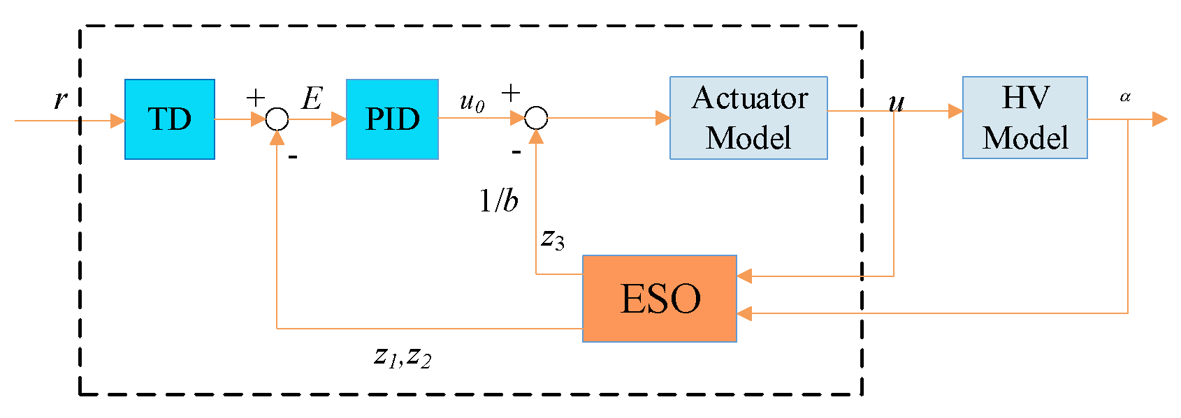
3. Construction of ADRC Based AFTC

Due to the existence of ESO, noise and disturbance are tolerated, to some extent. But when sensor faults occur, the PFTC cannot handle them. The information about sensor faults is needed for controller reconstruction to achieve AFTC. Thus, it is urgent to carry out fault identification to diagnose and identify sensor faults online.

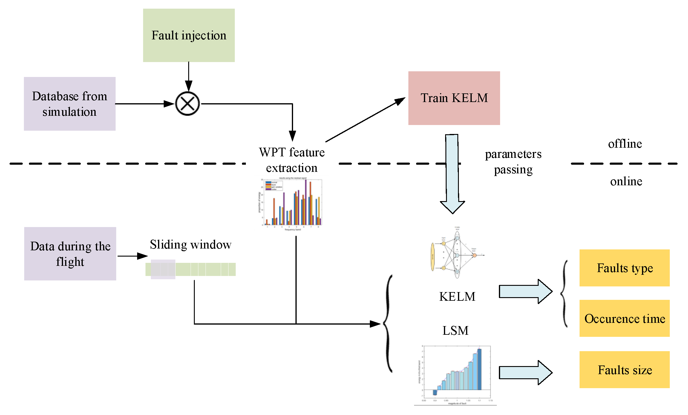
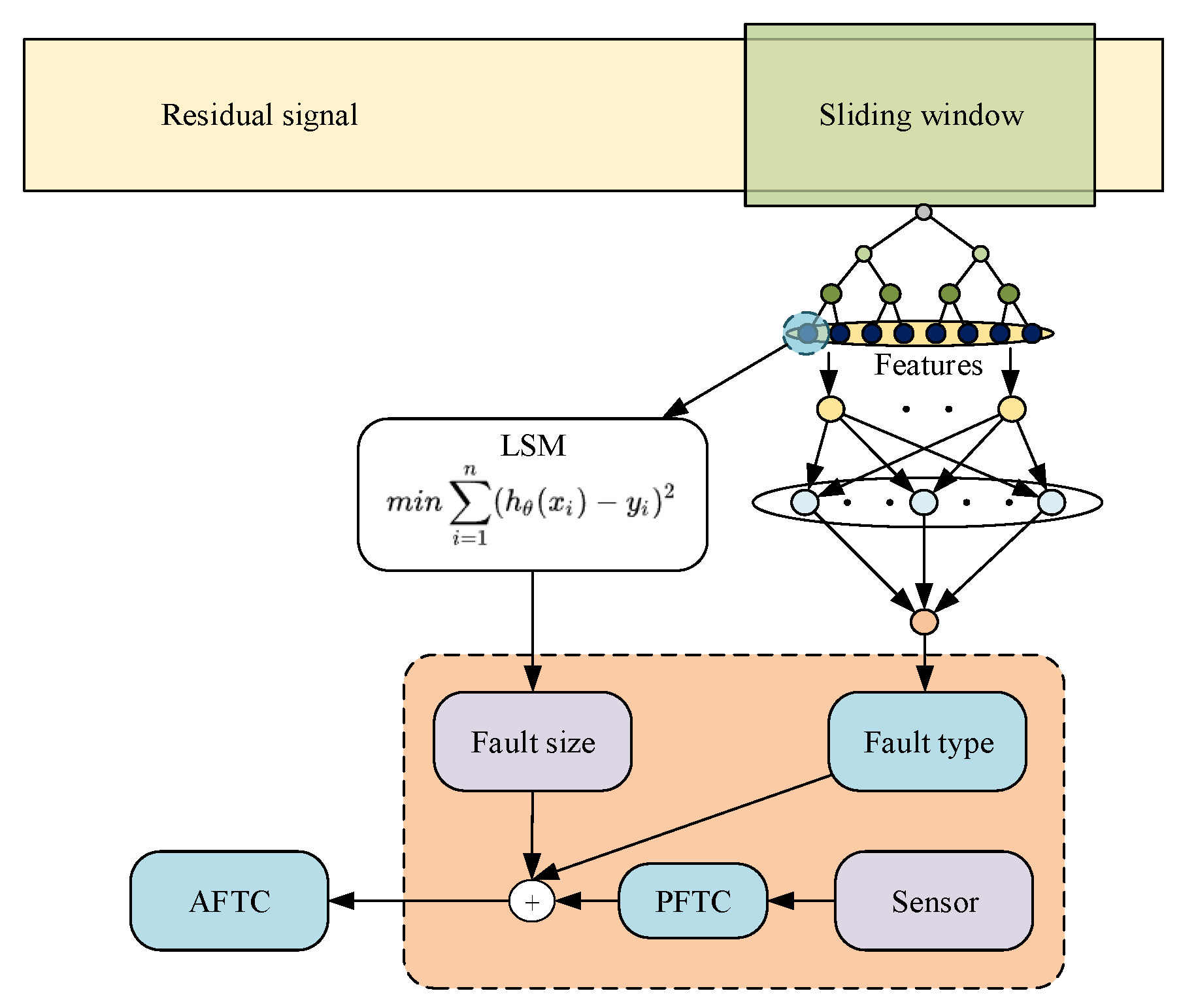
3.1. Fault Diagnosis and Identification

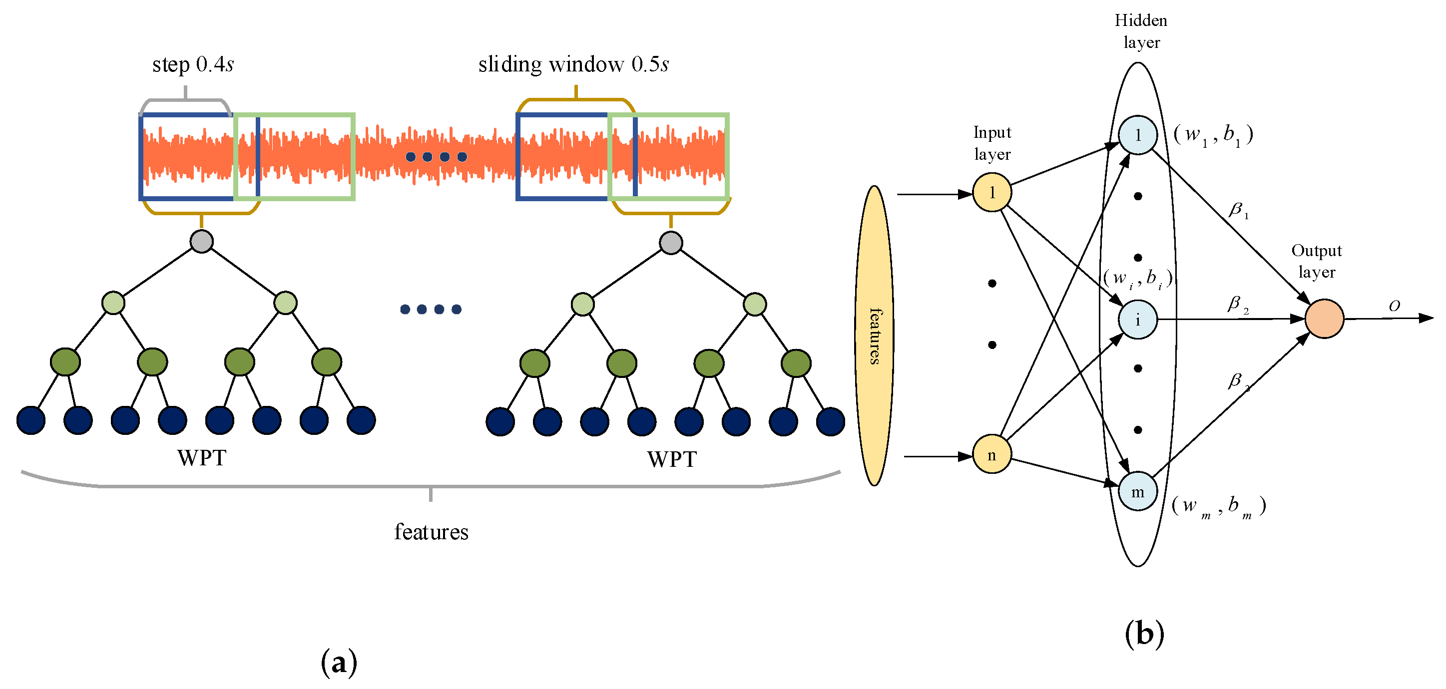
3.1.1. Fault Diagnosis by WPT and KELM

According to (2), ESO can be regarded as a reference model. Therefore, the residual between the observation of ESO and the output of NSHV contains the fault information. Efficient feature extraction is beneficial for fault diagnosis and evaluation. However, in the stage of reentry, NSHVs are affected by the severe environment. Considering maneuver and disturbance, the signal is characterized as a non-stationary signal. WPT is adopted to extract features, for wavelet transform’s unique advantages in processing non-stationary signals and its time-frequency feature processing ability. Sliding-window based feature extraction is adopted in view of real-time fault diagnosis. Figure 4a illustrates the structure of real-time fault identification.
Then, a classifier is used to classify sensor faults. Extreme Learning Machine (ELM) is a single hidden layer forward neural network, which has the advantage of calculation speed and accuracy. Figure 4b depicts the structure.
The output of ELM is O = i = 1 m β i g ( W i X i + b i ) , where g ( · ) is the activation function, W i is the weight, b i is the bias, and β i is the output weight. The output can be represented by the matrix O = H β , where H , β are the hidden layer’s output, and the output weights, respectively.
For ELM, once the W i , b i is given, the β can be calculated by β ^ = H + T , where H + is the Moore-Penrose pseudoinverse of H, T is the target output. Usually, a positive value I / C is added, where C is a user-defined parameter for calculating the output weights. Then the formula is rewritten as β ^ = H T ( I / C + H H T ) 1 T . The output of ELM is y ( x ) = h ( x ) β ^ , where h ( x ) is the hidden layer [30].
Further, KELM is raised to overcome the dimension disaster.
Ω E L M = H H T : Ω E L M i , j = h ( x i ) · ( x j ) = K ( x i , x j ) ,
where K ( x i , x j ) is a kernel function. In this paper, the Radial Basis Function (RBF) kernel is used. Finally, the output of KELM is obtained [31]:
f ( x ) = K ( x , x 1 ) K ( x , x N ) T ( I / C + Ω E L M ) 1 T
In this paper, the inputs of KELM are the features extracted by WPT and the outputs are types of sensor faults.

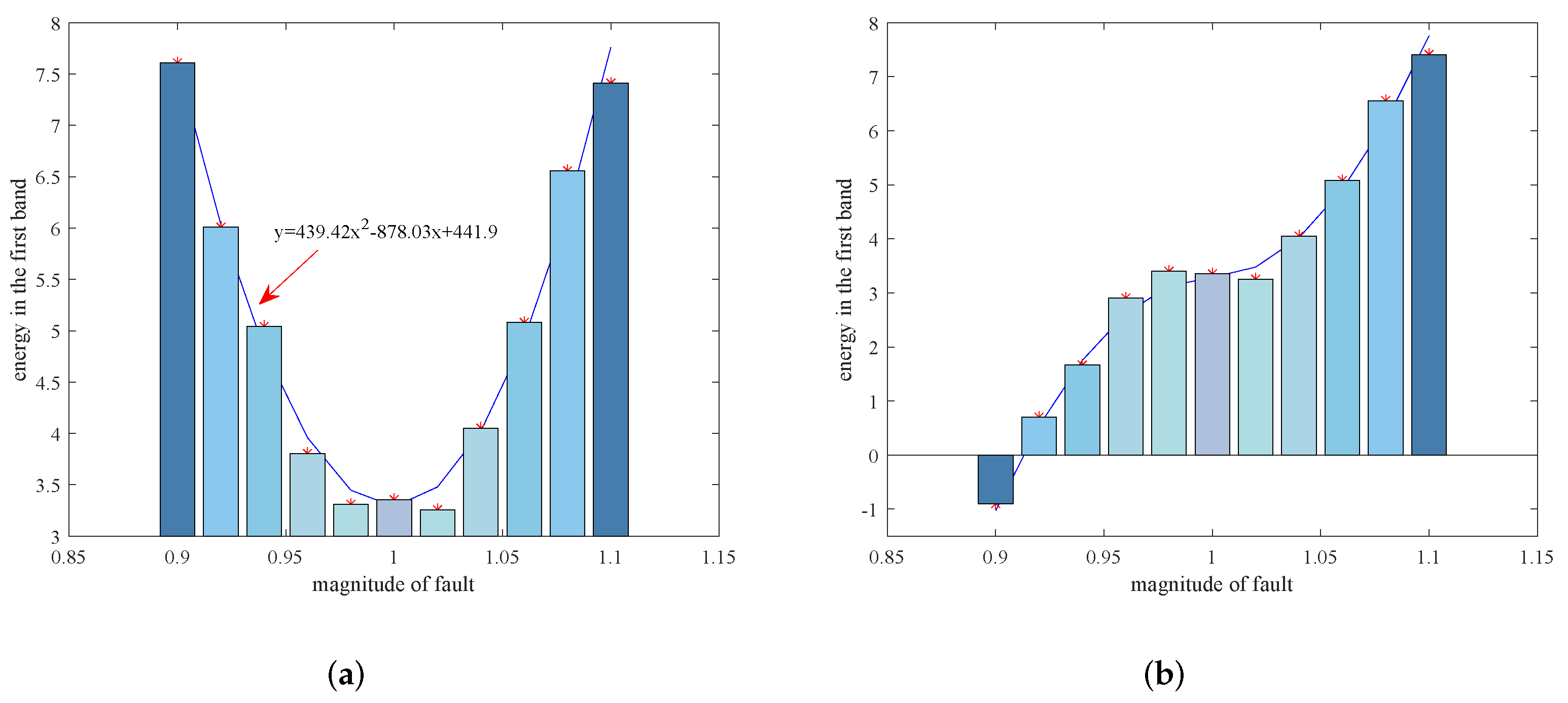
3.1.2. Joint Time-Frequency Analysis Based Fault Identification

Energy is extracted by WPT from the residual, and its expression is:
f 2 = | f ( x ) | 2 d x
In the low-frequency bands, the energy reflects the size of the sensor faults. Meanwhile, in the high-frequency ones, the energy is affected by sensor noise and the sensor faults. Least Square Method (LSM) is widely used in data fitting, for its simplicity and efficiency. And considering that the noise is concentrated in the high-frequency bands, it’s more accurate to use the energy in low-frequency bands to fit the size of sensor faults.

3.2. Policy of Controller Reconstruction

So far, Fault Diagnosis and Evaluation (FDE) is achieved by the proposed fault diagnosis method. And the whole AFTC structure is illustrated in Figure 5.
The AFTC is designed as:
α A F T C ( t ) = α ( t ) , 0 t t f α ( t ) , t f t t d α ( t ) + Δ F D E , t d t ,
where t f , t d are the time when faults occur and the time when the FDE unit determines the faults, respectively. α ( t ) is the output of the sensor. Δ F D E is the amount of compensation for sensor faults.

4. Simulation Results

To verify the effectiveness of the proposed AFTC method, simulations under the standard condition and fault conditions are presented. The mid-term of reentry segment of NSHVs is selected. In this stage, the NSHV adopts a large angle of attack for decelerating. The simulation conditions are H = 33.5 km , v = 15 Ma , α = 45 , q = 0 , and the angle of attack decreases to α = 35 , 2 s later, and the random noise μ = 0 . 5 is added to the data of the sensor. When the conditions are determined, the response is shown in the Figure 6.
The simulation shows that the NSHV can normally track the command with a raise time of 0.32 s, and the designed ESO observes the sensor output correctly under the fault-free condition. The sensor and actuator faults may occur at any time in the reentry process. To simplify the training process, faults are injected at 1.5 s during the simulation.

4.1. Simulations with Actuator Faults

According to the introduction of actuator faults model above, the gain variation fault K g = 0.9 and the stuck fault are injected separately.
It can be seen from Figure 7a,b that the designed PFTC has strong adaptability to the actuator gain variation fault. The steady-state time is only 0.2 s longer than the fault-free state. Meanwhile, the actuator stuck fault can be solved by redundant actuators, which is out of the range of this paper.

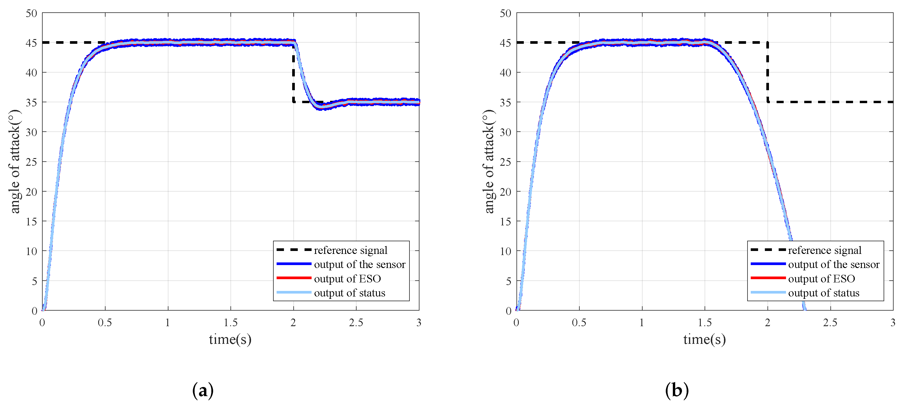
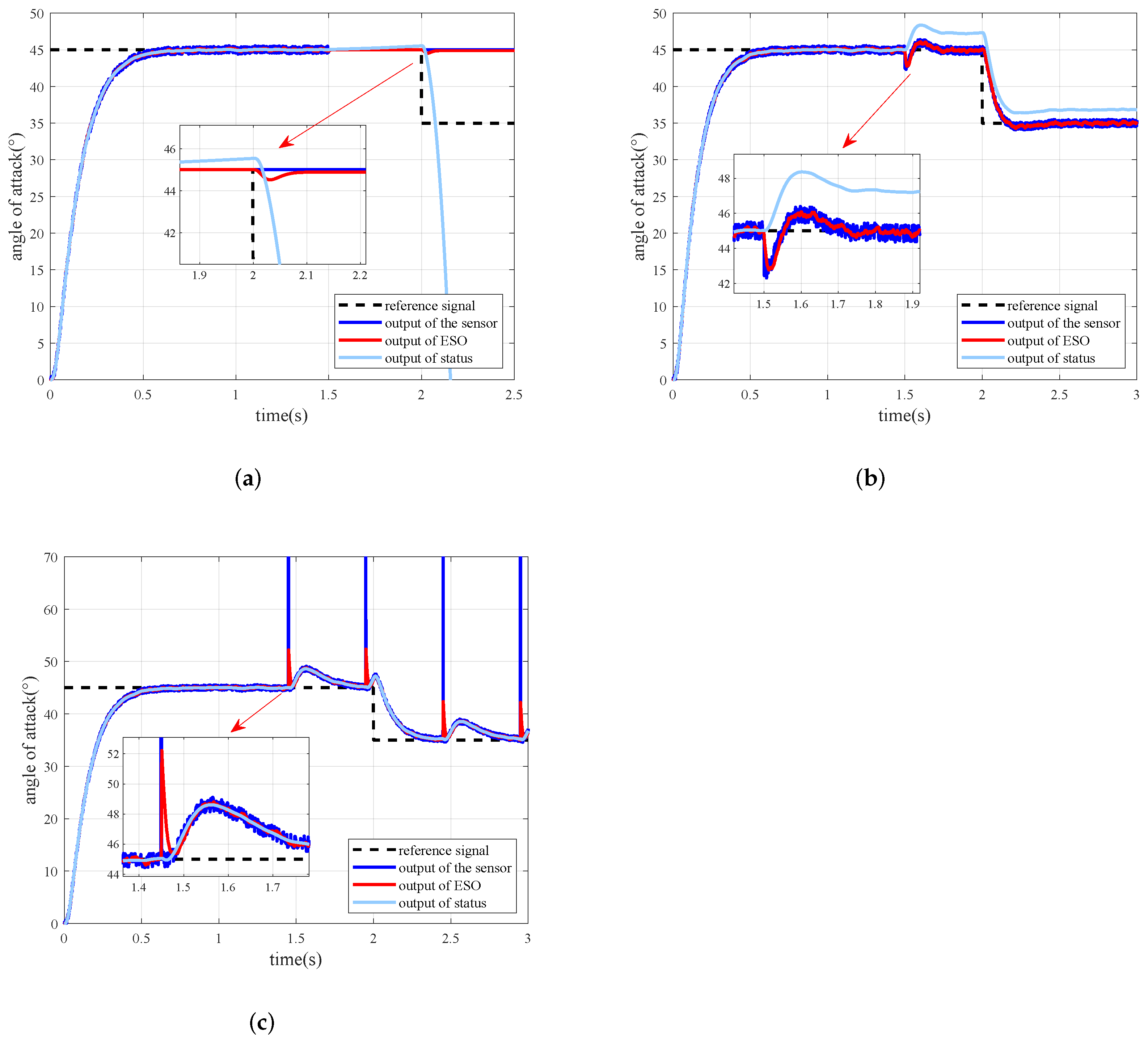
4.2. Simulations with Sensor Faults

The angle of attack of sensor fault states is compared with that of the fault-free state. The results of the stuck fault, gain variation faults and the outlier data fault are shown in Figure 8a, Figure 8b and Figure 8c, respectively.
The results show that the designed PFTC cannot handle sensor faults, although it has better performance in actuator faults. The NSHV cannot follow flight instructions properly because of the presence of faulty sensors. Sensor faults can reduce the flight quality and even seriously imperil the safety of NSHV.

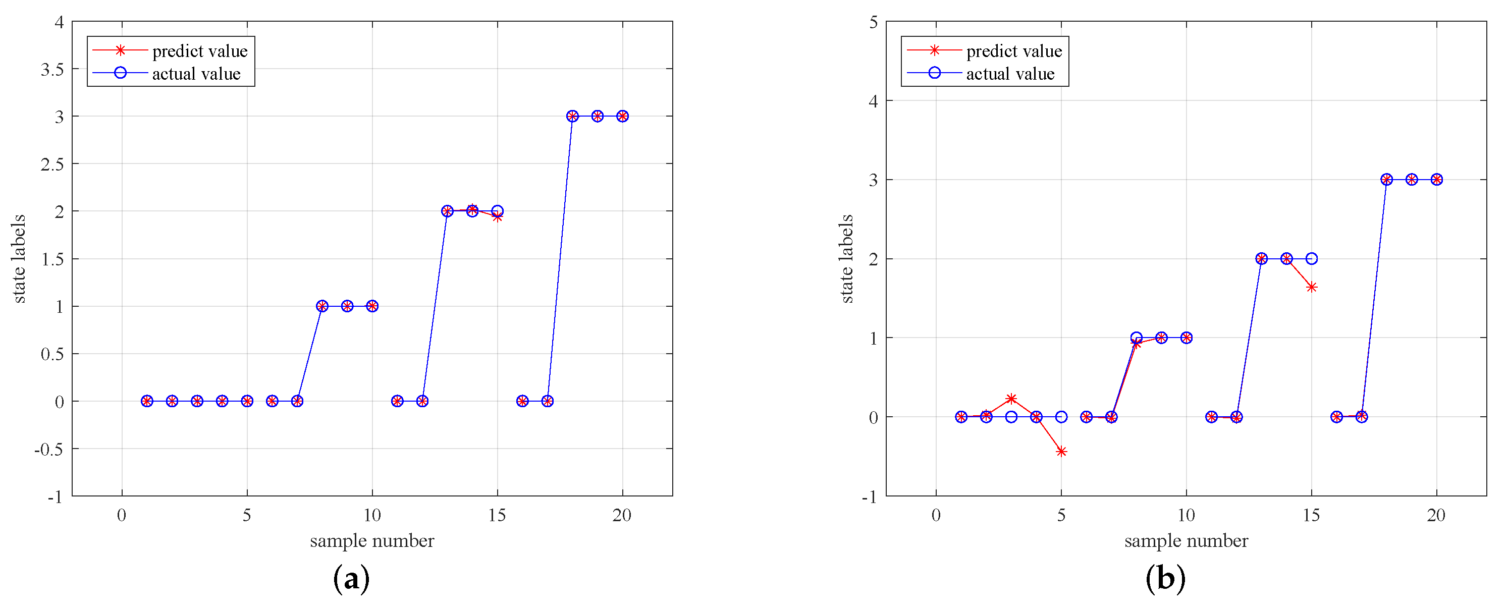
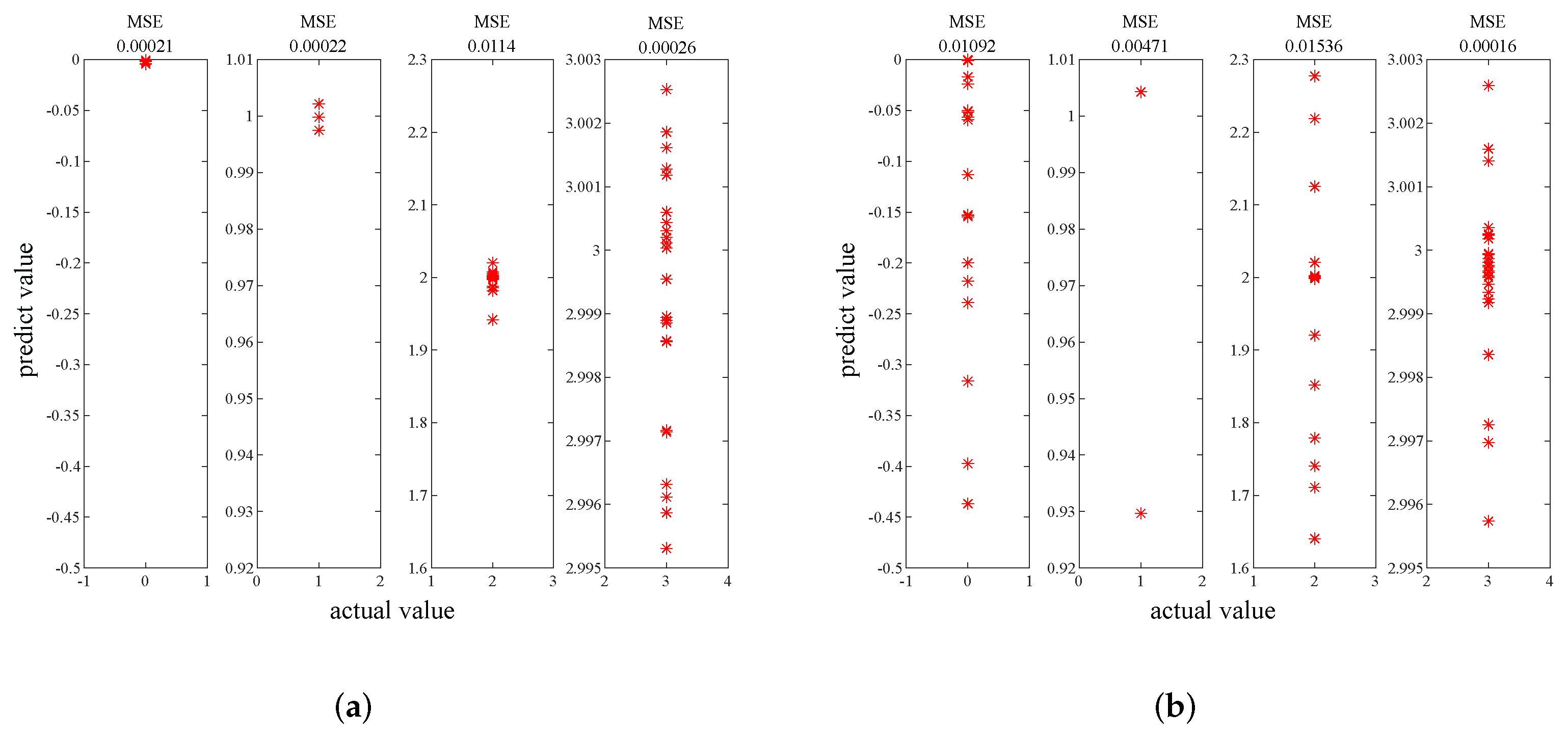
4.3. Simulations of the Proposed Fault Diagnosis Method

As our previous work showed, the energy distributions of diverse faults in different bands are various [3]. The energy caused by faults of different sizes shows a positive correlation with fault sizes, which can also get from the definition of energy (7).
For online FDE, a sliding window is adopted, with a 0.5 s sliding window and 0.4 s step time. The simulation result is shown in Figure 9a, where the labels 0, 1, 2, and 3 respectively represent the fault-free state, the stuck fault, the gain validation fault, and the outlier data fault.
To verify effectiveness of the proposed method, feature extraction and classification performed on the sensor output directly are adopted as the contrast method. It can be seen from results in Figure 9b that the contrast algorithm has greater uncertainty, especially in the fault-free state. This is because in the proposed method, the ESO estimates the total disturbance and counteracts the external interference, which is beneficial to improve the accuracy.
The distribution of multiple simulations is displayed in Figure 10a,b and Table 2. The Mean Squared Error (MSE) results show that except the outlier data fault, the proposed algorithm reduces the distribution of diagnostic results by up to 98%. The lower MSE indicates that the proposed method is more reliable. Although the MSE of the outlier data fault is slightly larger, the results of both methods are good enough in the diagnosis of the outlier data fault.
Furthermore, in terms of AFTC, it is necessary to know not only types of sensor faults but also sizes of faults. Energy in the low-frequency bands reflects sizes of the sensor fault. Under gain variation faults, as shown in Figure 11a, there is a quadratic correlation between the energy in the first band and gains, and the coefficients are calculated by LSM.
It should be noticed that the energy is symmetrically distributed, which is determined by the definition of residual energy. It can be solved by joint time-frequency analysis of the residual signal. Then, the energy can be redefined as:
E = s i g n ( K g 1 ) ( p 1 K g 2 + p 2 K g + p 3 ) + 2 ( K g < 1 ) · ( p 1 + p 2 + p 3 ) ,
where K g is the gain of the gain variation fault, p 1 , p 2 , p 3 are the coefficients calculated by LSM. The result is shown in Figure 11b.
According to (9), the gains can be solved by the energy:
x = p 2 + ξ ( r ) s q r t ( p 2 2 4 p 1 p 3 ) 2 p 1 ,
where ξ ( r ) is the sign of the residual signal. Above all, the fault identification with diagnosis delay less then 0.5 s is realized.

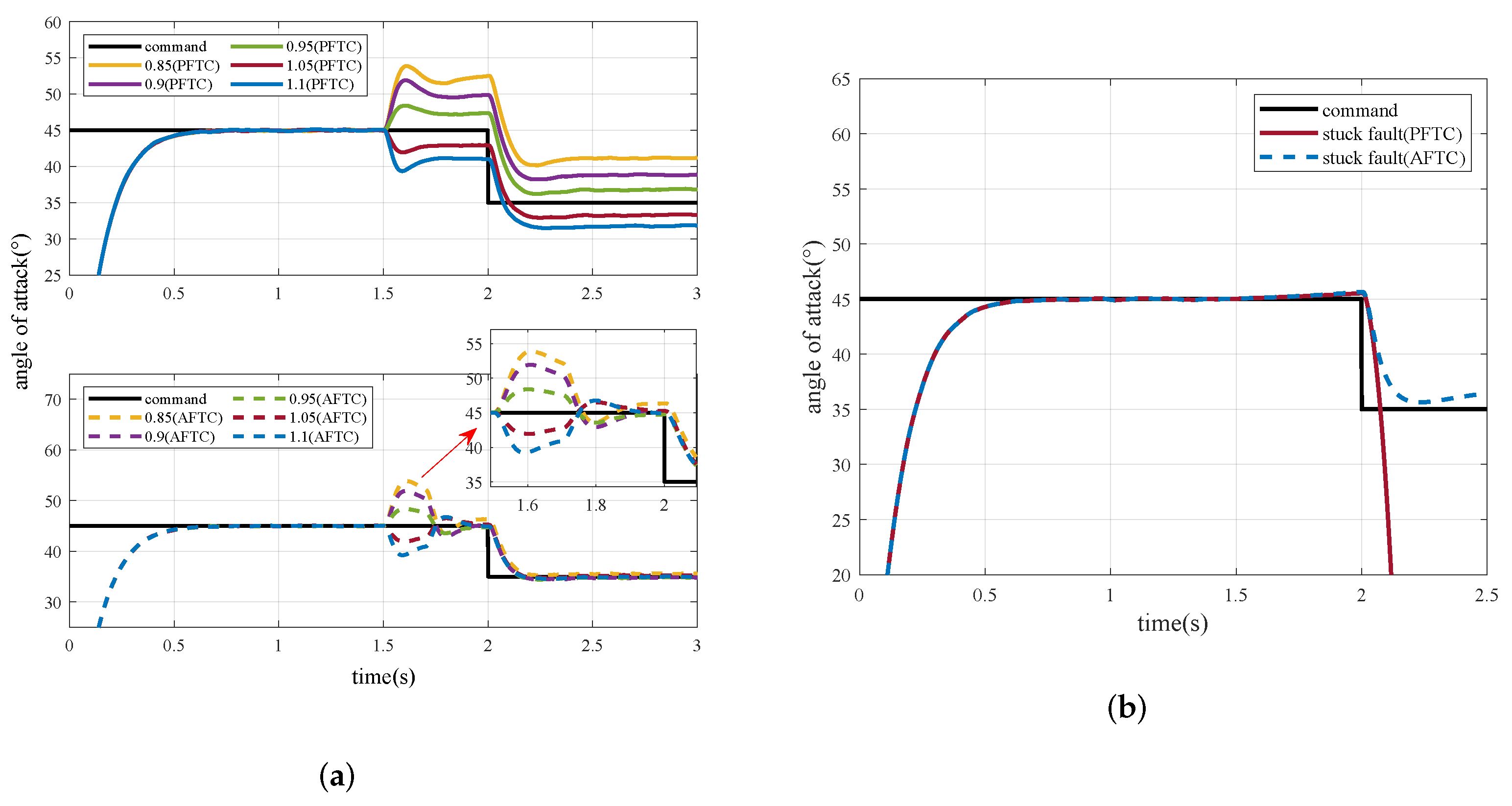
4.4. Simulations of AFTC

Once sensor faults occur during the flight, the fault diagnosis and identification unit generates information about the faults. According to the information, the strategy reconstruction is carried out by the AFTC proposed. The simulation results of different gain variation faults are described in Figure 11b and Table 3.
It can be seen that, when sensor faults occur, the PFTC strategy cannot counteract the wrong measurements. However, the NSHV adopted the proposed AFTC strategy can still follow the command correctly. The control command can be tracked correctly 0.4s after the fault occurs.
As the Figure 12b illustrates, under the stuck fault, the output of ESO is used as feedback to achieve security control to some extent. Compared with the PFTC strategy, the AFTC strategy has a stronger fault tolerant ability to the stuck fault. Command tracking can be maintained after the fault occurs, although it slowly diverges.

5. Conclusions

In this paper, a novel AFTC control strategy is proposed for NSHVs with actuator and sensor faults. An ADRC controller is adopted for command tracking and uncertainty compensation. To obtain accurate and real-time fault information, an estimation unit using ESO combined with KELM is presented. The ESO in ADRC is creatively used to generate residual signals to extract the features of different faults. Then, joint time-frequency analysis is adopted to estimate the sizes of faults. Combined ADRC with controller reconstruction strategy, AFTC is finally achieved. Actuator and sensor faults are discussed and analyzed to verify the effectiveness of the proposed reconfigurable control method. Simulation results show that the introduction of sliding window and KELM realizes real-time fault diagnosis, and the joint time-frequency analysis method makes fault identification possible. Finally, the NSHV adopted the proposed method can track the command precisely under the actuator and sensor faults. This paper provides new ideas for advanced active fault-tolerant control, especially for sensor faults.

Author Contributions

Conceptualization, J.S. and K.Z.; methodology, K.Z. and S.A.; software, K.Z.; validation, K.Z., S.A. and Y.L.; formal analysis, J.S. and X.X.; investigation, K.Z. and X.X.; resources, K.Z. and Y.L.; data curation, J.S.; writing—original draft preparation, K.Z.; writing—review and editing, K.Z.; visualization, K.Z.; supervision, J.S.; project administration, J.S.; funding acquisition, J.S. All authors have read and agreed to the published version of the manuscript.

Funding

This work was supported by the National Natural Science Foundation of China under Grants 61473015, 91646108 and 62073020.

Institutional Review Board Statement

Not applicable.

Informed Consent Statement

Not applicable.

Data Availability Statement

Not applicable.

Acknowledgments

The authors thank the colleagues for their constructive suggestions and research assistance throughout this study.

Conflicts of Interest

The authors declare no conflict of interest.

Abbreviations

The following abbreviations are used in this manuscript:
AFTCActive Fault-Tolerant Control
NSHVNear-Space Hypersonic Vehicle
ADRCActive Disturbance Rejection Control
KELMKernel Extreme Learning Machine
PFTCPassive Fault-Tolerant Control
AFTCActive Fault-Tolerant Control
FTCFault Tolerant Control
RCSReaction Control System
WPTThenWavelet Packet Transformation
ESOExtended State Observer
TDTracking Differentiator
RBFRadial Basis Function
LSMLeast Square Method
FDEFault Diagnosis and Evaluation
MSEMean Squared Error
Symbols
xhorizontal position, m
zvertical position, m
vvelocity, m/s
γ trajectory inclination angle, rad
α angle of attack, rad
mmass of NSHV, kg
ggravitational acceleration, m/s 2
Daerodynamic drag, N
T y propulsion, N
Yaerodynamic force, N
w y pitch angular rate, rad/s
I y moment of inertia for the y coordinate axes, kg · m 2
ldistance from the RCS to the center of mass, m
eresidual signal, rad
z 1 observation of the angle of attack, rad
z 2 observation of angular velocity of attack, rad/s
z 3 observation of total disturbance
β 1 , β 2 , β 3  tunable parameters
a 1 ( k ) estimated angle values of the current time, rad
a 1 ( k + 1 ) estimated angle values of the next time, rad
a 2 ( k ) derivative of a 1 ( k ) , rad/s
a 2 ( k + 1 ) derivative of a 1 ( k + 1 ) , rad/s
a * ( k ) desired signal, rad
T s sampling time, s
T c time constant, s
O ( t ) output of sensors or actuators
O f , s output under the stuck fault
O f , g output under the gain variation fault
O f , o output under the outlier data fault
t s time of stuck fault occur, s
t g time of gain variation fault occur, s
t o time of outlier data fault occur, s
K g gain variation fault size
δ outlier data fault size
f a l ( · ) the fault model
Ooutput of ELM
mnumber of neurons
β the output weights
g ( · ) activation function
W i weights of neurons
b i biases of neurons
X i inputs of ELM
Hhidden layer’s output
H + Moore-Penrose pseudoinverse of H
Ttarget output
Cuser-defined parameter
K ( · ) kernal function
α A F T C Control instruction of AFTC
α ( t ) output of the sensor
Δ F D E amount of compensation
t f time of fault occur
t d time when the fault is diagnosed
p 1 , p 2 , p 3 coefficients calculated by LSM
ξ ( r ) sign of the residual signal

References

  1. Gao, K.; Song, J.; Wang, X.; Li, H. Fractional-order proportional-integral-derivative linear active disturbance rejection control design and parameter optimization for hypersonic vehicles with actuator faults. Tsinghua Sci. Technol. 2020, 26, 9–23. [Google Scholar] [CrossRef]
  2. Zhai, R.; Qi, R.; Zhang, J. Compound fault-tolerant attitude control for hypersonic vehicle with reaction control systems in reentry phase. ISA Trans. 2019, 90, 123–137. [Google Scholar] [CrossRef] [PubMed]
  3. Kai, Z.; Jia, S.; Xinlong, W. ESO-KELM-based minor sensor fault identification. J. China Univ. Posts Telecommun. 2021, 28, 53. [Google Scholar]
  4. Jiang, B.; Zhao, J.; Qi, R.; Xu, D.; He, N. Survey of fault diagnosis and fault-tolerant control for near space vehicles. J. Nanjing Univ. Aeronaut. Astronaut. 2012, 44, 603–610. [Google Scholar]
  5. Hu, H.; Wang, B.; Cheng, Z.; Liu, L.; Wang, Y.; Luo, X. A novel active fault-tolerant control for spacecrafts with full state constraints and input saturation. Aerosp. Sci. Technol. 2021, 108, 106368. [Google Scholar] [CrossRef]
  6. Amin, A.A.; Hasan, K.M. A review of fault tolerant control systems: Advancements and applications. Measurement 2019, 143, 58–68. [Google Scholar] [CrossRef]
  7. Wang, B.; Yu, X.; Mu, L.; Zhang, Y. A dual adaptive fault-tolerant control for a quadrotor helicopter against actuator faults and model uncertainties without overestimation. Aerosp. Sci. Technol. 2020, 99, 105744. [Google Scholar] [CrossRef]
  8. Tahavori, M.; Hasan, A. Fault recoverability for nonlinear systems with application to fault tolerant control of UAVs. Aerosp. Sci. Technol. 2020, 107, 106282. [Google Scholar] [CrossRef]
  9. Zhang, Y.; Chen, Z.; Zhang, X.; Sun, Q.; Sun, M. A novel control scheme for quadrotor UAV based upon active disturbance rejection control. Aerosp. Sci. Technol. 2018, 79, 601–609. [Google Scholar] [CrossRef]
  10. Hu, K.; Chen, F.; Cheng, Z. Fuzzy Adaptive Hybrid Compensation for Compound Faults of Hypersonic Flight Vehicle. Int. J. Control Autom. Syst. 2021, 19, 2269–2283. [Google Scholar] [CrossRef]
  11. Wang, B.; Shen, Y.; Zhang, Y. Active fault-tolerant control for a quadrotor helicopter against actuator faults and model uncertainties. Aerosp. Sci. Technol. 2020, 99, 105745. [Google Scholar] [CrossRef]
  12. Rudin, K.; Ducard, G.J.; Siegwart, R.Y. Active fault-tolerant control with imperfect fault detection information: Applications to UAVs. IEEE Trans. Aerosp. Electron. Syst. 2019, 56, 2792–2805. [Google Scholar] [CrossRef]
  13. Xu, B.; Qi, R.; Jiang, B. Adaptive fault-tolerant control for HSV with unknown control direction. IEEE Trans. Aerosp. Electron. Syst. 2019, 55, 2743–2758. [Google Scholar] [CrossRef]
  14. Wu, T.; Wang, H.; Yu, Y.; Liu, Y.; Wu, J. Hierarchical fault-tolerant control for over-actuated hypersonic reentry vehicles. Aerosp. Sci. Technol. 2021, 119, 107134. [Google Scholar] [CrossRef]
  15. Yu, Y.; Wang, H.; Li, N. Fault-tolerant control for over-actuated hypersonic reentry vehicle subject to multiple disturbances and actuator faults. Aerosp. Sci. Technol. 2019, 87, 230–243. [Google Scholar] [CrossRef]
  16. Han, J.; Liu, X.; Wei, X.; Hu, X.; Zhang, H. Reduced-order observer based fault estimation and fault-tolerant control for switched stochastic systems with actuator and sensor faults. ISA Trans. 2019, 88, 91–101. [Google Scholar] [CrossRef]
  17. Zhai, D.; An, L.; Li, X.; Zhang, Q. Adaptive fault-tolerant control for nonlinear systems with multiple sensor faults and unknown control directions. IEEE Trans. Neural Netw. Learn. Syst. 2017, 29, 4436–4446. [Google Scholar] [CrossRef]
  18. Liu, Y.; Hong, S.; Zio, E.; Liu, J. Fault Diagnosis and Reconfigurable Control for Commercial Aircraft with Multiple Faults and Actuator Saturation. Aerospace 2021, 8, 108. [Google Scholar] [CrossRef]
  19. Ossmann, D.; Pusch, M. Fault Tolerant Control of an Experimental Flexible Wing. Aerospace 2019, 6, 76. [Google Scholar] [CrossRef] [Green Version]
  20. Lei, Y.; Yang, B.; Jiang, X.; Jia, F.; Li, N.; Nandi, A.K. Applications of machine learning to machine fault diagnosis: A review and roadmap. Mech. Syst. Signal Process. 2020, 138, 106587. [Google Scholar] [CrossRef]
  21. Liu, R.; Yang, B.; Zio, E.; Chen, X. Artificial intelligence for fault diagnosis of rotating machinery: A review. Mech. Syst. and Signal Process. 2018, 108, 33–47. [Google Scholar] [CrossRef]
  22. Li, X.J.; Yang, G.H. Adaptive fault-tolerant synchronization control of a class of complex dynamical networks with general input distribution matrices and actuator faults. IEEE Trans. Neural Netw. Learn. Syst. 2015, 28, 559–569. [Google Scholar] [CrossRef] [PubMed]
  23. Gao, Y.; Wu, L.; Shi, P.; Li, H. Sliding mode fault-tolerant control of uncertain system: A delta operator approach. Int. J. Robust Nonlinear Control 2017, 27, 4173–4187. [Google Scholar] [CrossRef]
  24. Li, H.; Gao, Y.; Shi, P.; Lam, H.K. Observer-based fault detection for nonlinear systems with sensor fault and limited communication capacity. IEEE Trans. Autom. Control 2015, 61, 2745–2751. [Google Scholar] [CrossRef]
  25. Dong, J.; Yang, G.H. Reliable state feedback control of T–S fuzzy systems with sensor faults. IEEE Trans. Fuzzy Syst. 2014, 23, 421–433. [Google Scholar] [CrossRef]
  26. Gao, K.; Song, J.; Yang, E. Stability analysis of the high-order nonlinear extended state observers for a class of nonlinear control systems. Trans. Inst. Meas. Control 2019, 41, 4370–4379. [Google Scholar] [CrossRef] [Green Version]
  27. Han, J. From PID to active disturbance rejection control. IEEE Trans. Ind. Electron. 2009, 56, 900–906. [Google Scholar] [CrossRef]
  28. Ai, S.; Song, J.; Cai, G. A real-time fault diagnosis method for hypersonic air vehicle with sensor fault based on the auto temporal convolutional network. Aerosp. Sci. Technol. 2021, 119, 107220. [Google Scholar] [CrossRef]
  29. Ai, S.; Song, J.; Cai, G. Diagnosis of Sensor Faults in Hypersonic Vehicles Using Wavelet Packet Translation Based Support Vector Regressive Classifier. IEEE Trans. Reliab. 2021, 70, 901–915. [Google Scholar] [CrossRef]
  30. Huang, G.B.; Zhu, Q.Y.; Siew, C.K. Extreme learning machine: A new learning scheme of feedforward neural networks. In Proceedings of the 2004 IEEE International Joint Conference on Neural Networks (IEEE Cat. No.04CH37541), Budapest, Hungary, 25–29 July 2004; Volume 2, pp. 985–990. [Google Scholar]
  31. Iosifidis, A.; Tefas, A.; Pitas, I. On the kernel extreme learning machine classifier. Pattern Recognit. Lett. 2015, 54, 11–17. [Google Scholar] [CrossRef]
Figure 1. Flowchart of the AFTC.
Aerospace 09 00237 g001
Figure 2. (a) Schematic drawing of NSHV; (b) the inertia and body coordinate.
Aerospace 09 00237 g002
Figure 3. The construction of ADRC. r is the desired angle of attack.
Aerospace 09 00237 g003
Figure 4. (a) Sliding-window based feature extraction; (b) structure of ELM.
Aerospace 09 00237 g004
Figure 5. The structure of AFTC.
Aerospace 09 00237 g005
Figure 6. Angle of attack under fault-free.
Aerospace 09 00237 g006
Figure 7. (a) Angle of attack under the gain variation fault; (b) angle of attack under the stuck fault.
Aerospace 09 00237 g007
Figure 8. (a) Angle of attack under the stuck fault; (b) angle of attack under the gain variation fault; (c) angle of attack under the outlier data fault (the maximum outputs of the outlier data are 90 ).
Aerospace 09 00237 g008
Figure 9. (a) Results of fault diagnosis using the method proposed; (b) results of fault diagnosis using the contrast method.
Aerospace 09 00237 g009
Figure 10. (a) Distribution of results using the method proposed; (b) distribution of results using the contrast method.
Aerospace 09 00237 g010
Figure 11. (a) Energy in the first band under different gain variation faults; (b) the relationship between the energy and the gain, considering the fault direction.
Aerospace 09 00237 g011
Figure 12. (a) Comparison of PFTC and AFTC under the gain variation faults; (b) comparison of PFTC and AFTC under the stuck fault.
Aerospace 09 00237 g012
Table 1. Capability of different control methods.
MethodAnti-InterferenceActuator Fault ToleranceSensor Fault Tolerance
PFTCpartly
Previous AFTC
AFTC proposed
Table 2. Distribution of results.
Fault TypeMSE Using the Proposed MethodMSE Using the Contrast Method
fault-free state0.000210.01092
stuck fault0.000220.00471
gain validation fault0.01140.01536
outlier data fault0.000260.00016
Table 3. Comparison of the control effects of PFTC and AFTC.
Fault SizeStatic Error Using PFTC ( )Static Error Using AFTC ( )
k = 0.856.280.49
k = 0.93.76−0.33
k = 0.951.71−0.2
k = 100
k = 1.05−1.820.14
k = 1.1−3.31−0.14
Publisher’s Note: MDPI stays neutral with regard to jurisdictional claims in published maps and institutional affiliations.

