Fault Detection of Aero-Engine Sensor Based on Inception-CNN

Abstract

The aero-engine system is complex, and the working environment is harsh. As the fundamental component of the aero-engine control system, the sensor must monitor its health status. Traditional sensor fault detection algorithms often have many parameters, complex architecture, and low detection accuracy. Aiming at this problem, a convolutional neural network (CNN) whose basic unit is an inception block composed of convolution kernels of different sizes in parallel is proposed. The network fully extracts redundant analytical information between sensors through different size convolution kernels and uses it for aero-engine sensor fault detection. On the sensor failure dataset generated by the Monte Carlo simulation method, the detection accuracy of Inception-CNN is 95.41%, which improves the prediction accuracy by 17.27% and 12.69% compared with the best-performing non-neural network algorithm and simple BP neural networks tested in the paper, respectively. In addition, the method simplifies the traditional fault detection unit composed of multiple fusion algorithms into one detection algorithm, which reduces the complexity of the algorithm. Finally, the effectiveness and feasibility of the method are verified in two aspects of the typical sensor fault detection effect and fault detection and isolation process.

1. Introduction

As the measuring element of the aero-engine control system, the function of the sensor is fundamental and essential for the system. However, with the increasing control demand and the increasing complexity of the control system, new requirements are put forward for the number and reliability of sensors, and in the poor working environment of aero-engine sensors, faults are difficult to avoid [1,2]. According to statistics, sensor faults cover more than 80% of faults in the aero-engine control system [3], so the fault detection and isolation (FDI) of aero-engine sensors are vital to improving the reliability of aero-engine control systems.

At present, the FDI methods of aero-engine sensors can be divided into two types: model-based and signal-based. The main idea of the model-based method is to establish the mapping relationship between the actual input and output of the controlled object by analyzing the physical characteristics of the controlled object and then analyzing the residuals between the output of the actual system and the output of the model for diagnosis and isolation [4]. The prominent representatives are the Kalman filter [5,6,7,8,9,10], particle filter [11], etc. Based on the model method, sensor fault detection becomes very simple under the premise of accurate model mapping. However, the complexity of actual controlled objects is the difficulty of its practical application.

Signal-based methods directly analyze signals through reliability analysis or machine learning, among which machine learning has made significant progress in the field of sensor FDI. Regarding fault identification based on one-dimensional sensor signals, literature [12] expands the one-dimensional signals of a single sensor into two-dimensional data. It inputs them into a CNN for fault detection through time series misalignment. However, this approach has poor randomness and reliability for aero-engines with complex control systems and diverse working conditions. Therefore, the most common solution is to use the analytically redundant space information between multiple sensors to detect faults of single or multiple sensors. In literature [13,14,15], the support vector machine (SVM) algorithm is used to build a nonlinear mapping relationship between faulty sensors and healthy sensors. Finally, an appropriate threshold is selected for the predicted value of the algorithm to determine whether the sensor is faulty. The literature [16,17,18] used the Levenberg–Marquardt algorithm, Artificial Bee Colony algorithm, and adaptive method to optimize a BP neural network to construct the mapping relationship between sensors for banning SVM. All of the above methods have high accuracy for single-sensor fault diagnosis. However, for multi-sensor diagnosis, it is necessary to build multiple algorithm units and match them with a complex logical judgment method or fusion judgment algorithm to make its accuracy usable. As mentioned in reference [19], assuming that no more than three sensors fail simultaneously among the nine sensors, 84 multi-input multi-output generalized regression neural networks (MIMOGRNNs) should be constructed for fusion diagnosis. In literature [20,21], the structure of the self-associative neural network and the extreme learning machine algorithm are optimized and changed by the genetic algorithm, respectively, to achieve multi-sensor detection, but its detection accuracy is still far from the 95% specified in the literature [22].

In recent years, CNN, as an essential part of deep learning algorithms, has had many applications in different engineering fields. Especially in data-based prediction, CNN shows good performance due to its robust feature extraction ability. Literature [23] proposed a prediction model based on CNN and lion algorithm fusion; the model was improved by niche immunity and finally used in the short-term load prediction of electric vehicles; the optimized prediction model can allow the existence of deformed data and has good prediction performance. Literature [24] proposed an innovative hyperspectral remote sensing image classification method based on CNN. The parameter update of the model adopts an extreme learning machine; finally, the model’s accuracy has been verified on the remote sensing image Jiuzhaigou. Literature [25] proposed a prediction model for detecting power theft by combining the bidirectional gated recurrent unit and CNN. Compared with the multilayer perceptron, the long short-term memory network (LSTM), and the single gated recurrent unit, the model performs better in this application scenario. Moreover, in the field of power protection, the author proposes a deep hybrid neural network model that combines CNN and particle swarm optimization (PSO) in literature [26]. The model uses CNN as the feature extractor of the PSO algorithm, which aims to condense useful feature information in the original time series. Literature [27] proposed a one-dimensional CNN prediction model for the real-time detection of motor faults. The model has a simple structure, low hardware requirements, and a fast detection speed. Literature [28] uses CNN to predict the sound source of plate-like structures. Compared with stacked autoencoders, CNN can accept more information input and has a flexible information input method. In the literature [29], the author converts the vibration sensor signal of the motor into a three-dimensional feature matrix as the input of the CNN, and different sensors occupy different channel dimensions in the feature matrix. This paper provides ideas for the situation in which there are different kinds of feature data as CNN input. In the literature [30], the author used the output of the virtual sensor of the aero-engine physical model and the Kalman filter as the input of a one-dimensional CNN and realized the life prediction of the aero-engine. Compared with feed-forward neural networks (FNN) and LSTM, this method has smaller variance and higher accuracy in multiple predictions. In literature [31], the object detection deep learning algorithm YOLOv3 based on CNN is used. The prediction model built by this algorithm realizes the detection of the number of people in an air-conditioned room and reduces the energy consumption of the air conditioning. Literature [32] built a predictive model for power transformer and cyberattack fault diagnosis.

This paper proposes a convolutional neural network based on the inception block; the Inception-CNN uses the convolution layer and pooling layer to extract the analytical redundancy information between each sensor. Next, this information is used to adjust network parameters and predict the probability of individual sensor failures.

The innovations of this paper are as follows.

(1)

The construction of the forecasting model

Compared to the various signal-based methods mentioned above, Inception-CNN can take advantage of the characteristics of the inception block to incorporate more interphase information of sensors of different scales into the fault detection model, which is undoubtedly beneficial to the signal-based method. In addition, the method is based on the self-iterative characteristics of neural networks; thus, it does not require a tedious parameter optimization process, and can focus more on the construction of the network model itself.

(2)

Generation of fault datasets

Actual aero-engine sensor failure data are very sparse, which contradicts the large amount of training data required for deep learning algorithms. This paper generates sufficient data for training by the Monte Carlo simulation method.

(3)

The optimization of the forecasting model input

In this paper, the one-dimensional data of the sensor are converted into a two-dimensional feature matrix by the pan and regroup method. This method makes the extraction of sensor phase information more sufficient, and the prediction model’s accuracy is improved.

(4)

The optimization of the forecasting model details

The activation function and output mode of the predictive model are optimized so that the model can perform fault detection on all target sensors simultaneously, and the accuracy of the model is improved.

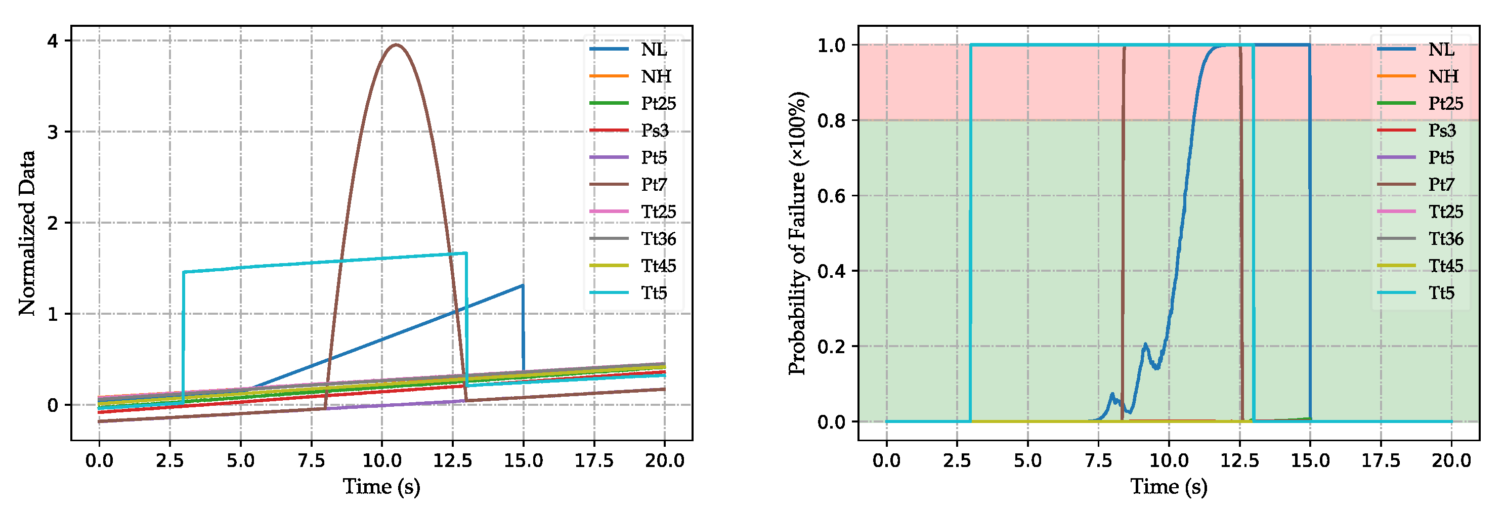
The rest of the paper is organized as follows: Section 2 introduces the research object of the prediction model in this paper and the construction of training data and validation data. Section 3 shows the various parts of the CNN and how they work and then shows the specific architecture of the Inception-CNN prediction model. Section 4 verifies the feasibility and effectiveness of Inception-CNN in terms of fault detection effect and FDI process, respectively. Section 5 concludes this paper.

2. Data Preparation

This paper takes a Geared Turbofan Engine (GTF) as the research object, which can be expressed as Equation (1):

$$\left[x_s^{\left(t\right)},x_v^{\left(t\right)}\right]=F\left(w^{\left(t\right)},{\theta }^{\left(t\right)}\right)$$

(1)

Among them, w is the operating condition, including height (alt), flight speed (Mach), power lever angle (PLA), etc. $\theta$ is a health parameter. $x_s$ is a measurable physical property, including the values of each sensor, and $x_v$ is an unobservable physical quantity.

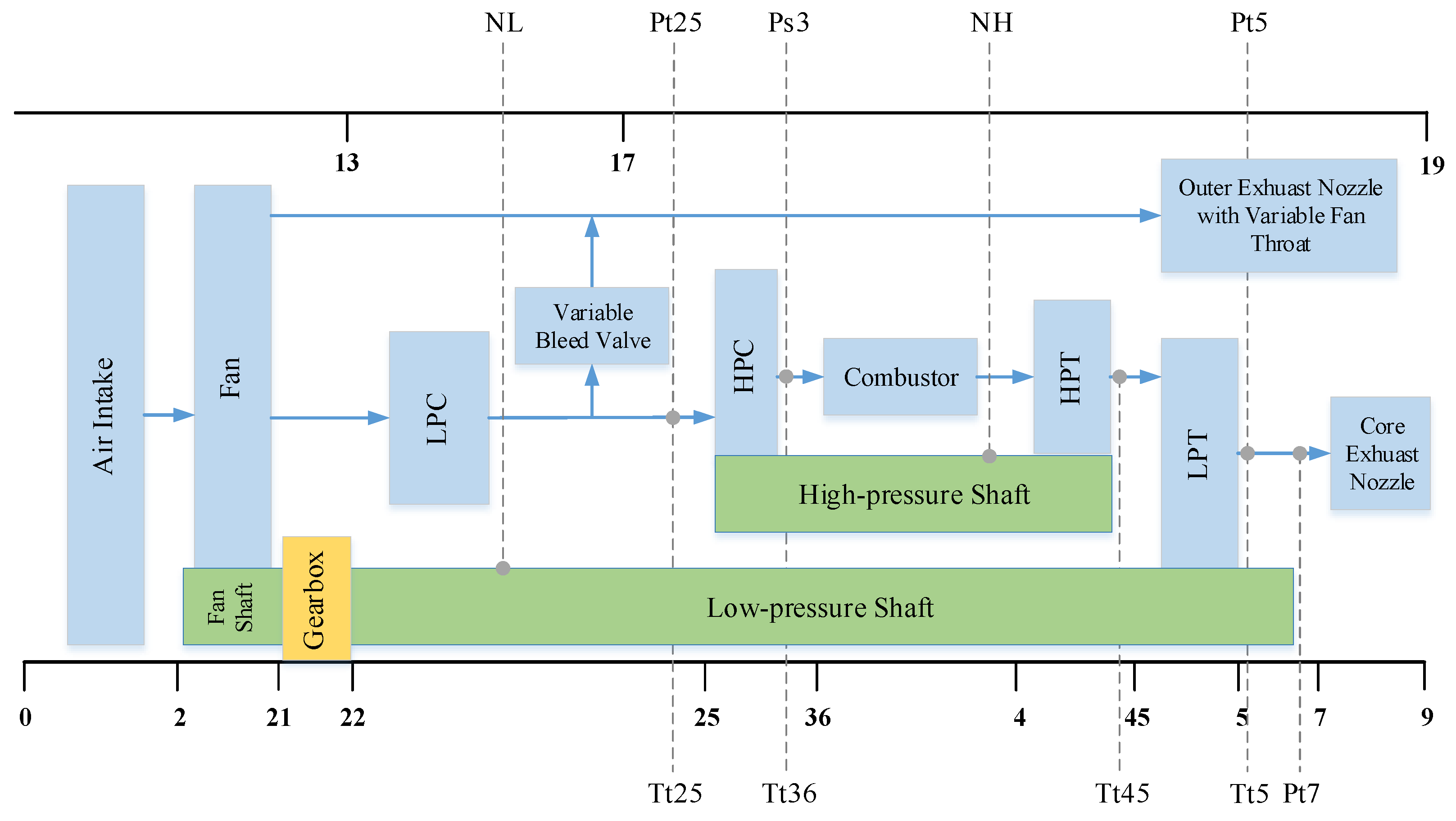
Due to the limitation of calculation conditions, this paper only studies the ground operation of an aero-engine, namely height = 0 and speed = 0. Ten sensors are selected as the research object of this paper, as shown in Equation (2), and the cross-section position of the aero-engine is shown in Figure 1.

$$x_{sensor}=\left[\begin{array}{c}\mathrm{NL},\mathrm{NH},\mathrm{Pt}25,\mathrm{Ps}3,\mathrm{Pt}5,\mathrm{Pt}7,\mathrm{Tt}25,\mathrm{Tt}36,\mathrm{Tt}45,\mathrm{Tt}5\end{array}\right]$$

(2)

In this paper, the method is tested and verified by the GTF model of NASA/T-MATS master [33] in the simulation environment of Matlab/Simulink2021a.

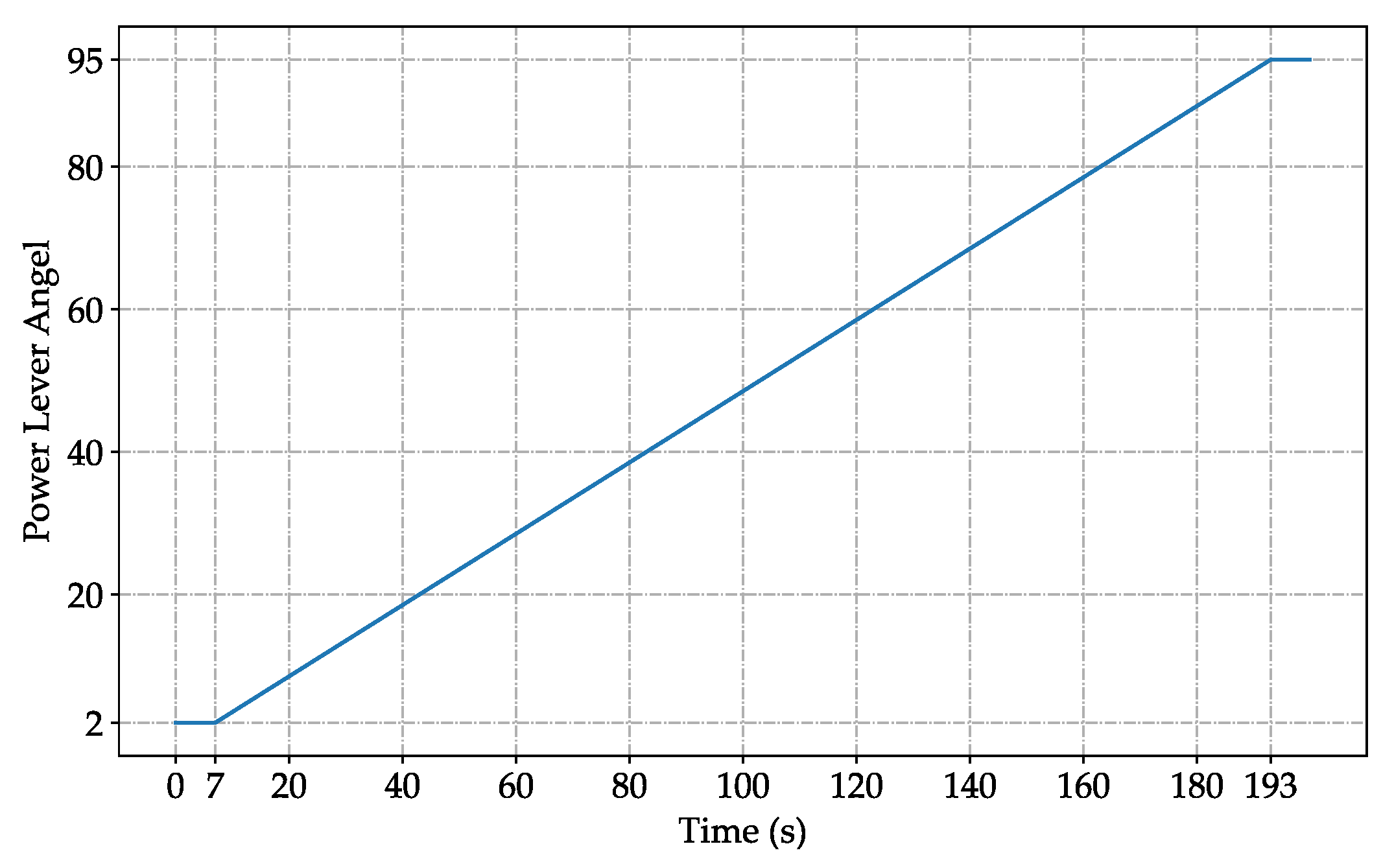
By referring to the verification method of the civil turbofan engine fault diagnosis system proposed by Donald et al. [34,35], the Monte Carlo simulation method is used to generate the training and verification data set of the neural network. Firstly, the power lever angle (PLA) of the healthy running engine model is given, as shown in Figure 2, and sensor data $x_{sensor}$ are derived. Then, ten sensor data $x_{sensor}$ are randomly disturbed by the normal distribution, as shown in Equation (3).

$$y_{sensor}^i=x_{sensor}^i+{\alpha }^{i}XX\sim N\left(0,1\right)$$

(3)

The coefficient ${\alpha }^i$ is determined by the average $Mean\left(x_{sensor}^i\right)$ of the input sensor value.

In the training data set and validation data set, the data point that exceeds 5% of the original value of the sensor is set as the fault point. For example, if $|{\left(y_{sensor}^i\right)}_j-{\left(x_{sensor}^i\right)}_j|>0.05\times {\left(x_{sensor}^i\right)}_j$, sensor i is considered a failure at j data points, whereas sensor i is considered to have no failure. 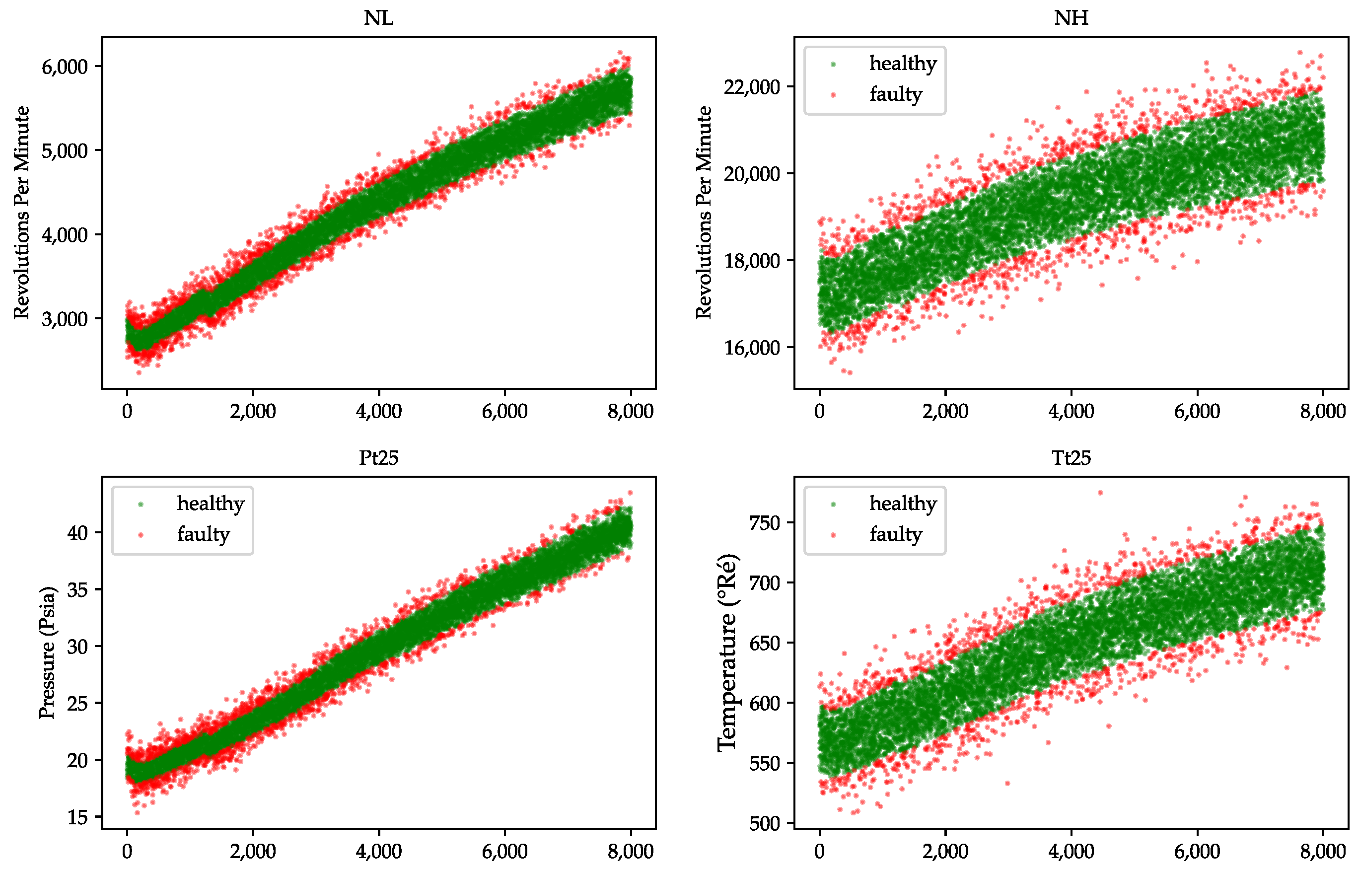Since class imbalance can adversely affect network training, this paper adjusts ${\alpha }^i$ to reduce the gap between faulty and healthy data points and loops to generate data multiple times. Since the probability of failure of more than three sensors at the same time is extremely small, and the redundant information between the sensors decreases with the increase in the number of simultaneously failed sensors, the data points where more than three sensors fail at the same time ${\sum }_{i=1}^{10}\phi \left[{\left(x_{sensor}^i\right)}_j\right]>3$ are deleted. The scatter plot of a small part of the value of NL, NH, Pt25, and Tt25 sensors after adding disturbance is shown in Figure 3, where the abscissa represents the label of the data points.

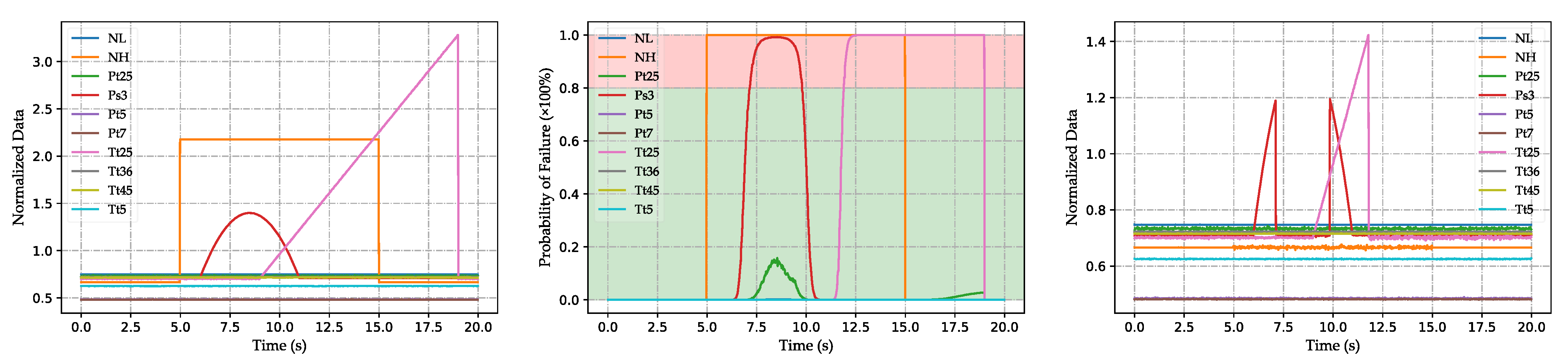
In the final method verification link, we adjust the coefficient ${\alpha }^i$ to ensure that the sensor data $y_{sensor}$ are equivalent to the actual engine data collected and filtered, add the typical faults shown in

Table 1. Typical sensor failure.

Type of Failure	Cause of Failure
Impulse	Random disturbances, surges, sparks, etc.
Drift	Sensor component deterioration, etc.
Bias	Bias current, bias voltage, etc.

, and change the PLA to verify the neural network’s generalization performance.

3. Introduction to Inception-CNN

3.1. Introduction to CNN

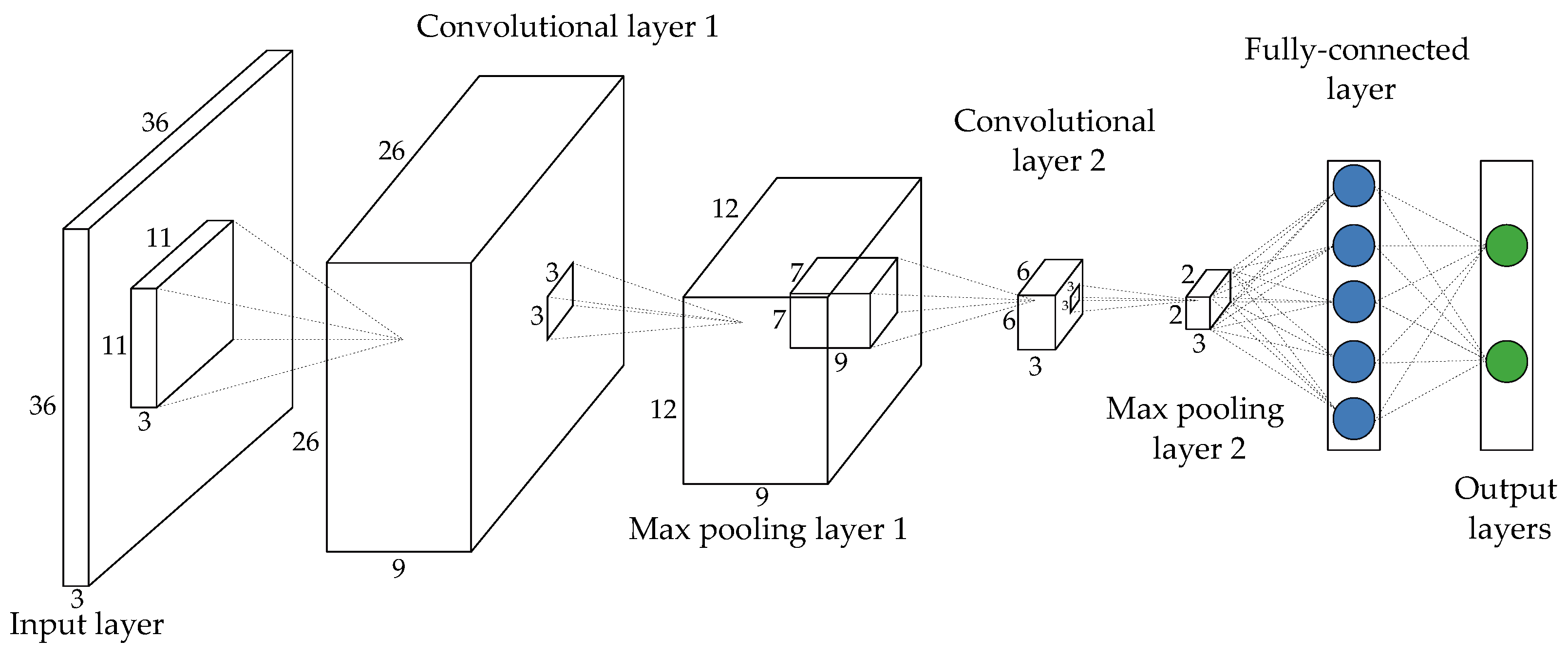
As a transformed form of multilayer perceptron, the convolutional neural network (CNN) was developed based on studies on the visual cortex of cats [36]. It was initially applied in the field of image recognition. Now, CNN has become a hot spot in many research fields. A typical CNN consists of convolutional layers, pooling layers, and fully connected layers, as shown in Figure 4.

Convolutional layers extract local features of the input data by a perceptual structure and reduce the number of parameters of the CNN by sharing weights. The pooling layer merges adjacent data into a single datum, reduces the dimensionality of the data, speeds up the calculation, and prevents the overfitting of the parameters. The fully connected layer is the basic unit of the BP neural network, which generates output based on the feature data extracted by the previous layer.

3.2. The Basic Module of CNN

The input of each node of the convolutional layer is only the local features of the previous layer, and the convolution kernel is used to convert the subnode matrix of the current layer into a unit node matrix with unlimited channel dimensions in the next layer. Under normal circumstances, the convolution layer generally only converts the channel dimension of the input data and adopts the method of edge zero-padding to ensure that the length and width of the input data remain unchanged. For example, the convolution kernel transforms the matrix of $m_1\times n_1\times k_1$ into $1\times 1\times k_2$ as Equation (4).

$$g\left(i\right)=f\left({\Sigma }_{x=1}^{m_1}{\Sigma }_{y=1}^{n_1}{\Sigma }_{z=1}^{k_1}{a}_{x,y,z}\times w_{x,y,z}^i+b^i\right),0<i⩽k_2$$

(4)

Among them, $g\left(i\right)$ represents the value of the ith identity matrix of this node, and $a_{x,y,z}$ represents a certain length and width of the convolution kernel sampling in the input matrix of this node. The interception matrix with the channel dimension $\left(x,y,z\right)$. $w_{x,y,z}^i$ represents the convolution kernel weight value matrix corresponding to the ith unit matrix, $b^i$ represents the bias value corresponding to the ith unit matrix, and f represents the activation function. In this paper, Scaled Exponential Linear Units (SELU) is selected as the activation function, which normalizes the data distribution and ensures that the gradient will not explode or disappear during the training process. The SELU activation function can be expressed as Equation (5):

$$selu\left(z\right)=\lambda \left\{\begin{array}{c}zz>0\hfill \\ \alpha e^z-\alpha z⩽0\hfill \end{array}\right.$$

(5)

where z represents the output value of the convolution operation, and $\lambda$ and $\alpha$ are constants, $\lambda \cong 1.051$, $\alpha \cong 1.673$.

Pooling layers sample the data by sliding the pooling kernel. Unlike convolutional layers, pooling layers generally only change the length and width of the input matrix. The most common types of pooling layers are max pooling and average pooling. The process of converting the $m_1\times n_1\times k_1$ matrix to $1\times 1\times k_1$ by max layer pooling is as Equation (6):

$$g\left(i\right)=Subsampling\left(a_{x,y}^i\right),0<x⩽m_1,0<y⩽n_1,0<i⩽k_1$$

(6)

Among them, $g\left(i\right)$ represents the value of the ith unit matrix of this node, and $a_{x,y}^i$ represents the interception matrix of a length and width $\left(x,y\right)$ sampled by the pooling kernel when the input matrix of this node corresponds to the ith unit matrix. The pooling layer reduces the data size, speeds up computation, and prevents parameter overfitting without losing data features.

Finally, the network expands the feature matrix extracted by the convolutional and pooling layers into a one-dimensional vector, which is input to the fully connected layer and produces an output based on these features.

3.3. The Calculation Process of CNN

Minimizing the loss function $L\left(W,b\right)$ as much as possible is the goal of neural network training, where W and b represent the weights and bias parameters in the neural network, respectively. The loss function consists of two parts: the first part is the residual between the output value and the expected value, and the second part is the regularization loss caused by overfitting, which is regulated by the parameter $\theta$. The loss function can be expressed as Equation (7):

$$L\left(W,b\right)=E\left(W,b\right)+\frac{\theta }{2}{W}^{T}W$$

(7)

This paper uses the Stochastic Gradient Descent plus Momentum (SGDm) as the solver to update the CNN parameters. Through the back-propagation of the loss function, the trainable parameters of each layer in the CNN can be updated layer by layer. The mathematical representations are as Equations (8) and (9):

$$W_i=W_{i-1}+m_i,m_i=\left(\eta \frac{\partial L\left(W_i,b_i\right)}{\partial W_i}+\beta m_{i-1}\right)$$

(8)

$$b_i=b_{i-1}+m_i,m_i=\left(\eta \frac{\partial L\left(W_i,b_i\right)}{\partial b_i}+\beta m_{i-1}\right)$$

(9)

where $\eta$ is the learning rate, and $\beta$ is the momentum coefficient.

3.4. Inception Block

Although a deep neural network can be abstractly considered the superposition of several neural networks, different network architectures and choices of hyperparameters will make a huge difference in the performance of deep neural networks. Furthermore, with the deepening of the network, the interpretability of the deep neural network becomes worse. A deep neural network with good performance often needs to explore the design intuition formed in this field for many years, so it is vital to master and use the previous exploration results.

The inception block is the basic module of the GoogLeNet network architecture proposed in 2014 [37], and GoogLeNet prevailed in the ImageNet competition that year.

Earlier convolutional neural networks are often series architectures. The size of the convolution kernel is also very different, such as from $1\times 1$ to $11\times 11$, etc. However, the inception block parallels convolutional layers with convolution kernels of different sizes in order to have the ability to extract correlated features at different scales. It has been shown that using convolution kernels of different sizes is beneficial for feature extraction.

In addition, deeper neural networks are often helpful to improve prediction accuracy. However, deep networks also bring the risk of gradient disappearance, which will cause the model to fail to converge eventually. Furthermore, due to the exponential increase in computing parameters in deeper networks, the demands on computing equipment are further increased. The inception block can reduce the network computing parameters effectively.

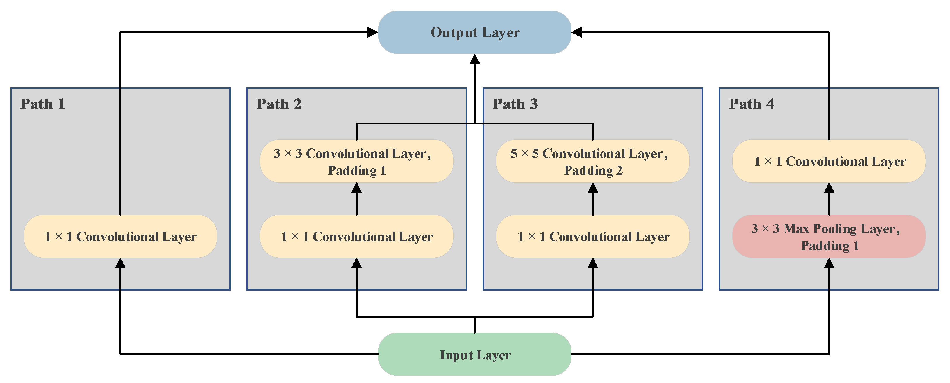
As shown in Figure 5, the inception block consists of four parallel paths. The first three paths use convolutional layers with kernel sizes $1\times 1$, $3\times 3$, and $5\times 5$ to extract information from different spatial sizes. The two paths in the middle first perform $1\times 1$-convolution on the input to reduce the number of channels and reduce the complexity of the model. The fourth path uses a pooling layer with a pooling kernel size $3\times 3$ and then uses a $1\times 1$ convolution kernel to vary the number of channels. All four paths use appropriate padding to match the height and width of the input and output and, finally, join the output of each line in the channel dimension and form the output of the inception block. In the inception block, the adjusted hyperparameters are mainly the number of output channels per layer.

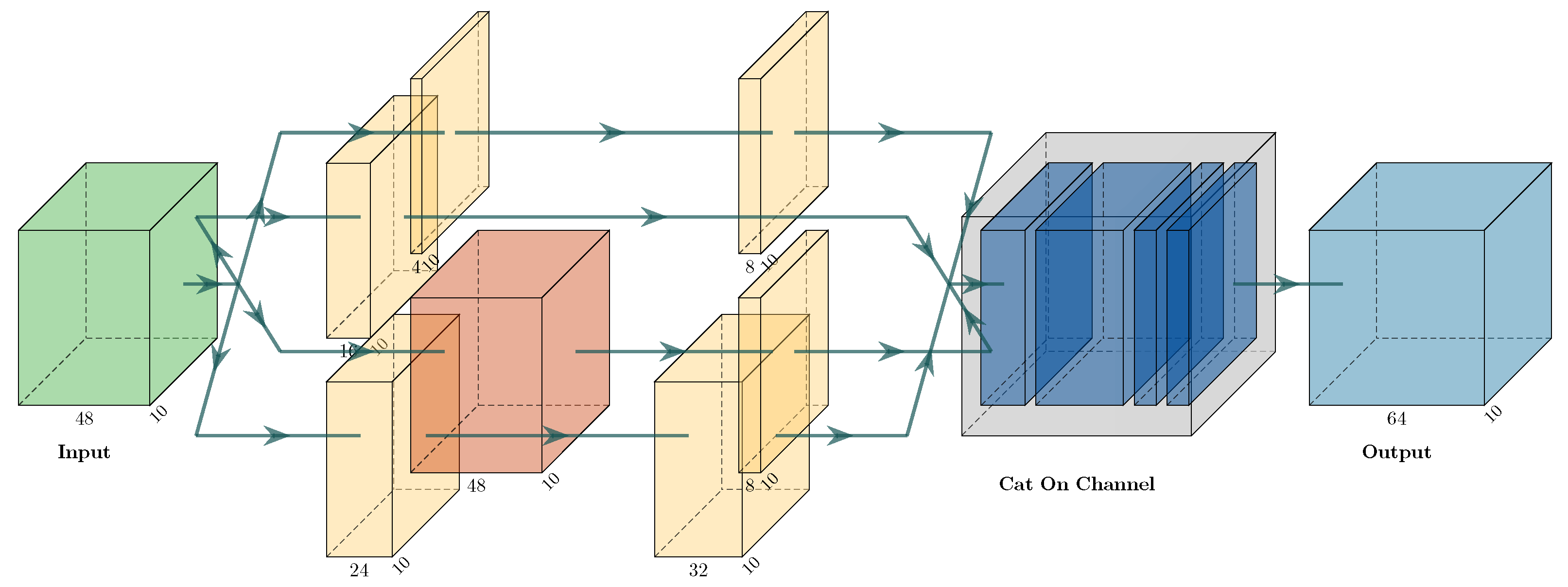
The specific representation of the first inception block used in this paper is shown in Figure 6. The input is an $10\times 10$ matrix with a channel number of 48, which passes through four paths, respectively. After the different convolution pooling operations, which are shown in Figure 5, the number of channels is changed and merged into the output matrix in the channel dimension, as the following input to one layer of the neural network.

3.5. Architecture of Inception-CNN

Considering that the convolution kernel has the characteristics of the local receptive field, for one-dimensional data, it is difficult for the convolution kernel to extract the interphase features of the data with a large separation distance. In order to fully extract the relevant features between sensor signals, this paper performs two-dimensional expansion and recombination of the original data before the data are input into the neural network. That is, the size of the data $1\times n$ is expanded to $n\times n$.

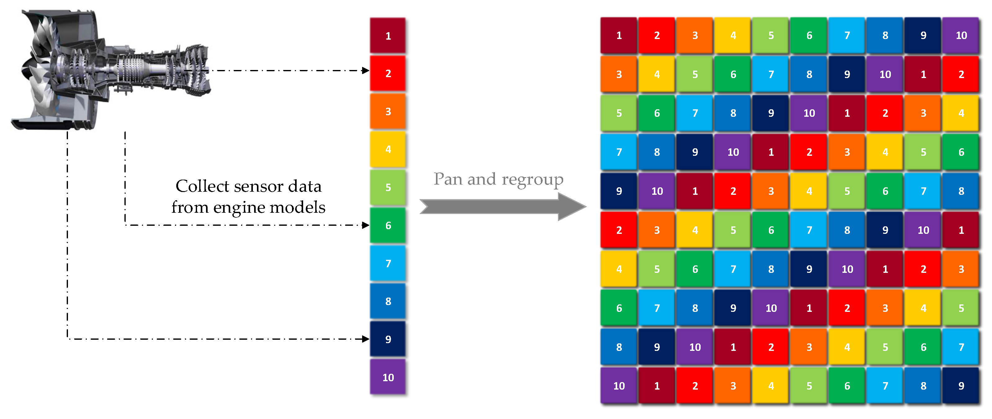
As shown in Figure 7, first, through the method described in Section 1, a one-dimensional sensor data set is obtained by collecting data from the engine model. Different colored and numbered squares represent data from different sensors. Then, the one-dimensional data group is expanded into a two-dimensional data group while rearranging the data through the data translation operation. For example, the second row of the two-dimensional data group in the figure is obtained by shifting the original one-dimensional data group by two units.

Suppose that a convolution kernel of size three is used to extract the interphase features of the sensor data. In this case, it is impossible to extract the interphase features of the sensor data with an interval greater than 3 in the original one-dimensional data set. However, it can be done in the two-dimensional data set after translation expansion.

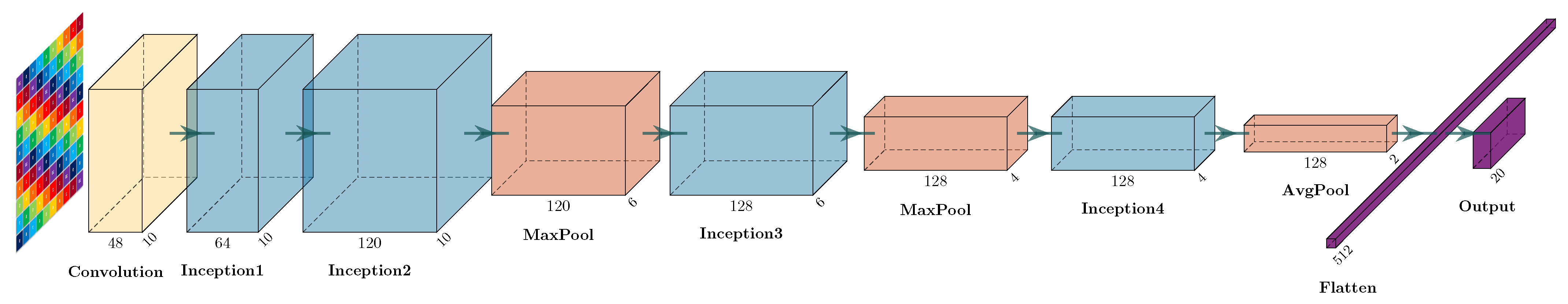
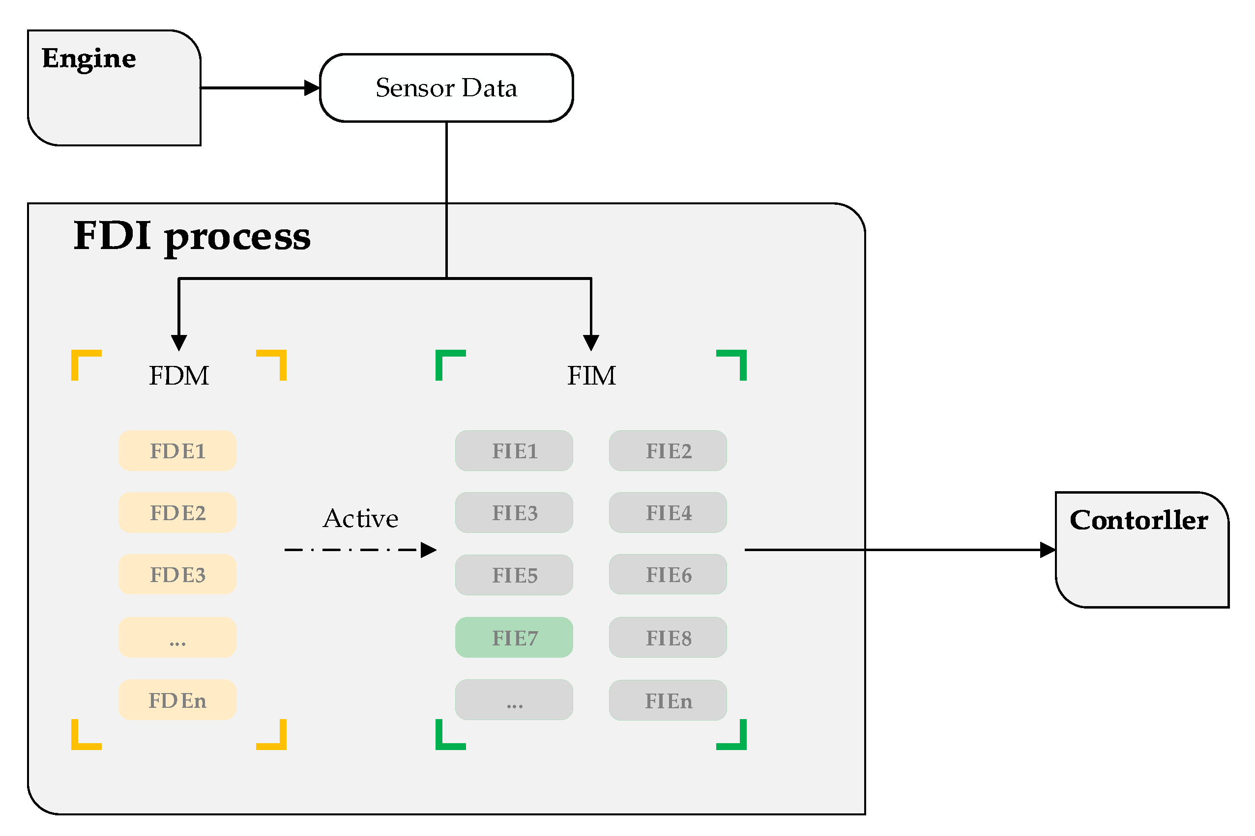
Since the neural network model requires a large amount of data for parameter updating, this paper adopts the operating mode of offline training and online detection. The Inception-CNN architecture is shown in Figure 8. A large amount of perturbed and labeled sensor data is used as the network input during offline training, and the network parameters are updated. During online diagnosis, the data format is kept unchanged, the sensor data that match the actual situation are input to the network, and the prediction is made based on the updated parameters during offline training.

As shown in Figure 8, the two-dimensional sensor data set expanded by translation is input into the network and passes through one convolution layer, four inception blocks, two max pooling layers, and one average pooling layer. The first convolutional layer has 48 convolution kernels of size $3\times 3$, which converts the original data of size $1\times 10\times 10$ into a feature response matrix of size $48\times 10\times 10$. The pooling kernel size of all pooling layers in the network is $2\times 2$. After the last average pooling, the three-dimensional matrix is converted to a one-dimensional vector with no information loss. Finally, the extracted feature response vector is input to the fully connected layer and produces an output with 20 nodes.

The parameters of the four inception block convolution kernels and pooling kernels are shown in Figure 5. The changed hyperparameters are only the number of channels output by each layer. The channel parameters are shown in

Table 2. Channel parameters for each inception block.

Serial Number	Path 1	Path 2	Path 3	Path 4	Number of Output Channels
1	16	24.32	4.8	48.8	64
2	32	32.48	8.24	64.16	120
3	48	24.52	4.12	120.16	128
4	40	28.56	6.16	128.16	128

.

3.6. Loss Function

In the traditional multiclassification problem using neural networks, if the classification category is n, it is necessary to construct an n-dimensional one-hot encoding vector to represent the category, and network output nodes are required. For example, in the three-classification problem, the three one-hot vectors $\left[1,0,0\right]\left[0,1,0\right]\left[0,0,1\right]$ represent three different categories. It can be seen that one element in the vector is 1, and the others are 0.

$$y_i=\frac{e^{a_i}}{{\sum }_{k=1}^C{e}^{a_k}}\forall i\in 1\cdots C$$

(10)

Equation (10) is the softmax function expression, where a is the output value of the last fully connected layer. By calculating the natural logarithm, the softmax function converts the network’s output into the probability of each category on the one-hot encoding, i.e., $\left[p1,p2,p3\right]$. Among them, $p1+p2+p3=1$. The softmax function is widely used in multi-classification problems due to its fit with one-hot encoding and its ability to widen the difference between categories in most cases.

However, in the sensor fault detection problem in this paper, due to the assumption that multiple sensors fail simultaneously, the detection vector output by the network will present multiple 1s at the same time. For example, $\left[1,0,1,0,0,0,0,0,0,0\right]$ means that the NL sensor and the Pt25 sensor fail simultaneously, so the softmax function is no longer applicable in the network, and the sensor failure probability is only calculated during model validation.

For multi-classification problems, a combination of the softmax function and cross-entropy loss function is often used. The expression of the cross-entropy loss function is as Equation (11).

$$E\left(W,b\right)=-\frac{1}{N}\sum _i\sum _{c=1}^M{y}_{ic}log\left(p_{ic}\right)$$

(11)

Among them, M is the number of categories, y is the symbolic function, i is the batch data size, and p is the predicted probability of the category, which is the output of softmax. Since softmax is no longer applicable, the output of the fully connected layer a is replaced with p.

There are two types of individual sensors, faulty and healthy, and one-hot encoding is constructed for each sensor separately, so the number of final output nodes of Inception-CNN is $10\times 2$, a total of 20 output nodes. Every two nodes constitute a prediction unit of the sensor. The output value of the cross-entropy loss function of each prediction unit is accumulated as a total loss value for the back-propagation of the network.

In summary, the loss function expression used in this paper is as Equation (12):

$$E\left(W,b\right)=\sum _{j=1}^{10}\left(-\frac{1}{N}\sum _i\sum _{c=1}^M{y}_{ic}log\left(a_{ic}\right)\right)$$

(12)

where j is the number of the prediction unit, and a is the output of the last fully connected layer of the network.

4. Validation and Analysis

4.1. Training the Networks

The Inception-CNN and other comparative neural networks in this paper are trained in the simulation environment of Python3.9/Pytorch1.10.1. The rest of the non-neural network machine learning algorithms are trained in the simulation environment of Matlab2021a. For the data set constructed in Section 1, the accuracy of some neural networks during the training process is shown in Figure 9, and the accuracy of each algorithm when it converges is shown in

Table 3. Performance comparison of Inception-CNN and other algorithms.

Algorithm	Activation Function	Loss Function	Accuracy at Convergence
Gaussian Naive Bayes	\	\	67.81%
Cubic SVM	\	\	73.35%
Cosine KNN	\	\	75.54%
Gaussian SVM	\	\	78.14%
BP Neural Networks	ReLU (Rectified Linear Unit)	MSE	82.72%
Simple 4-Tier CNN	ReLU	MSE	85.41%
Inception-CNN	ReLU	MSE	91.82%
Inception-CNN	SELU	MSE	92.13%
Inception-CNN	SELU	Cross-Entropy	95.41%

:

Each neural network sets the same training hyperparameters. The learning rate is 0.0001, and the batch size is 256.

It can be seen from Table 3 that the accuracy of the neural network is significantly improved compared to other non-neural network algorithms. For example, a simple BP neural network improves the accuracy by 4.58% compared to the best-performing Gaussian SVM in a non-neural network. Compared with the simple BP neural network, the accuracy of the simple four-layer CNN network is increased by 2.69%, so the CNN fits this data set better than other algorithms; thus, the improved CNN was chosen as the fault detection algorithm in this paper.

Figure 9 takes Epoch as the abscissa and the ordinate as the accuracy of each network on the test data set. The first three CNN networks use the mean square error (MSE) loss function, and the fourth network uses the improved cross-entropy loss function in the paper. It can be seen from Figure 9 and Table 3 that the CNN based on the inception block has a rapid increase in accuracy and a higher upper limit than the simple four-layer CNN. After replacing the traditional ReLU activation function with the SELU activation function, the convergence time of the network is reduced, and the training time is reduced by approximately 60%. After replacing MSE with the improved cross-entropy loss function in this paper, the network’s sensitivity to wrong predictions is improved. The accuracy rate rises faster, and the accuracy during convergence is 3.28% higher than that of Inception-CNN using the MSE loss function. The final accuracy of Inception-CNN used in this paper is 95.41%.

4.2. Typical Sensor Failure Validation

The typical sensor fault verification link is divided into two parts. On the one hand, it tests the detection effect of Inception-CNN itself for typical faults, and on the other hand, it verifies the effectiveness of the network in the FDI process.

Excellent generalization performance is an important indicator to measure the performance of neural network models. For the research content of this paper, even if the data set for training Inception-CNN is only composed of a simple slope response after adding disturbance, it is still expected to have good prediction results for all ground operating conditions of the engine model.

Therefore, in a typical sensor failure verification process, the steady-state or transition-state conditions used for each verification are different.

4.2.1. Validation of Fault Detection Effect

First, we verify the case of a single fault and simultaneous multiple faults in the steady state of the engine.

A single sensor failure occurs at a steady state, as shown in Figure 10. Under different steady-state conditions, the impulse, drift, and bias fault are added to the NL, Pt25, and Tt36 sensor, respectively. It can be seen from the figure that when the fault probability is 80% as the threshold, the injected impulse fault, drift fault, and bias fault are identified by the fault detection system after delays of around 0.1 s, 4.2 s, and 0 s, respectively. The drift fault has a relatively long detection delay due to the small offset in the early stage when the fault occurs. In addition, after injecting faults, the failure probabilities of other sensors without faults are all below 6% and fluctuate much less than the threshold.

As described in Section 1, when constructing the neural network training data, this paper removes data points where more than three sensors fail simultaneously. Thus, the simultaneous failure of up to three sensors is the assumption of this paper.

The simultaneous failure of multiple sensors in a steady state is shown in Figure 11. Under a specific steady-state condition, the bias, impulse, and drift fault are injected into the NH, Ps3, and Tt25 sensor at approximately 5 s, 6 s, and 9 s, respectively. The detection delay of each fault is around 0 s, 1.6 s, and 2.5 s, respectively. Among them, the delay of drift fault detection is still caused by insufficient offset in the early stage of fault occurrence. As can be seen from the figure on the right, although multiple faults occur simultaneously, it does not affect the accurate identification of a single fault by the fault detection system, and the detection delay is hardly affected by multi-sensor faults. Among the non-faulty sensors, the failure probability of the Pt25 sensor fluctuates up to approximately 19%, but it is still far below the failure probability threshold.

Next, we verify the case of a single fault and simultaneous multiple faults in the transition state of the engine.

A single sensor failure occurs at a transition state, as shown in Figure 12. Under different transition state conditions, the impulse, drift, and bias fault were injected into the NH, Pt5, and Tt45 sensor, respectively. The situation is similar to a single sensor failure in a steady state. The detection system identifies each fault after delaying by 0.1 s, 2.6 s, and 0 s, respectively. It can be seen that the performance of Inception-CNN in the transition state and steady state is comparable.

The simultaneous failure of multiple sensors in a transition state is shown in Figure 13. Under a specific steady-state condition, the drift, impulse, and bias fault are injected into the NL, Pt7, and Tt5 sensor at approximately 5 s, 3 s, and 9 s, respectively. The detection delay of each fault is approximately 5.9 s, 0.2 s, and 0 s, respectively. The delay in detecting drift faults is due to the fact that the injected drift fault offset is small, and the drift fault itself has the characteristic of slowly increasing the offset.

4.2.2. Validation in the FDI Process

As shown in Figure 14, the FDI process consists of a fault detection module (FDM) and a fault isolate module (FIM). The FDM contains fault detection estimators (FDE) running in real time, and the FIM contains fault isolate estimators (FIE) that require the output of the FDM to activate. The essence of each estimator is a method of fault detection or isolation. The Inception-CNN proposed in this paper is an FDE in the FDI process.

The Gaussian process regression algorithm is used to build the FIE module.

Due to space limitations, the FDI process verification is only carried out for the simultaneous failure of multiple sensors. First, we verify the FDI flow of the engine at a steady state.

As shown in Figure 15, when multiple sensors fail simultaneously in a steady state, FDM effectively activates FIM through the built-in Inception-CNN. After the FDI process, the injected fault offsets of drift, impulse, and bias faults are reduced by around 81%, 61%, and 100%, respectively, which correspond to different faults’ detection delays. The lower impulse fault offset reduction percentage is the lower injected impulse fault offset.

When multiple sensors fail simultaneously in the transition state, it is similar to the steady state, as shown in Figure 16. After the FDI process, the drift, impulse, and bias fault offsets were reduced by 76%, 56%, and 100%, respectively. The effectiveness of Inception-CNN in the FDI process is verified.

5. Conclusions

In this paper, a convolutional neural network based on an inception block is proposed and utilized for aero-engine sensor fault detection. The traditional detection unit composed of multiple fusion algorithms is simplified into one detection algorithm, which mainly solves the problems of traditional sensor FDI methods with many parameters and complex systems.

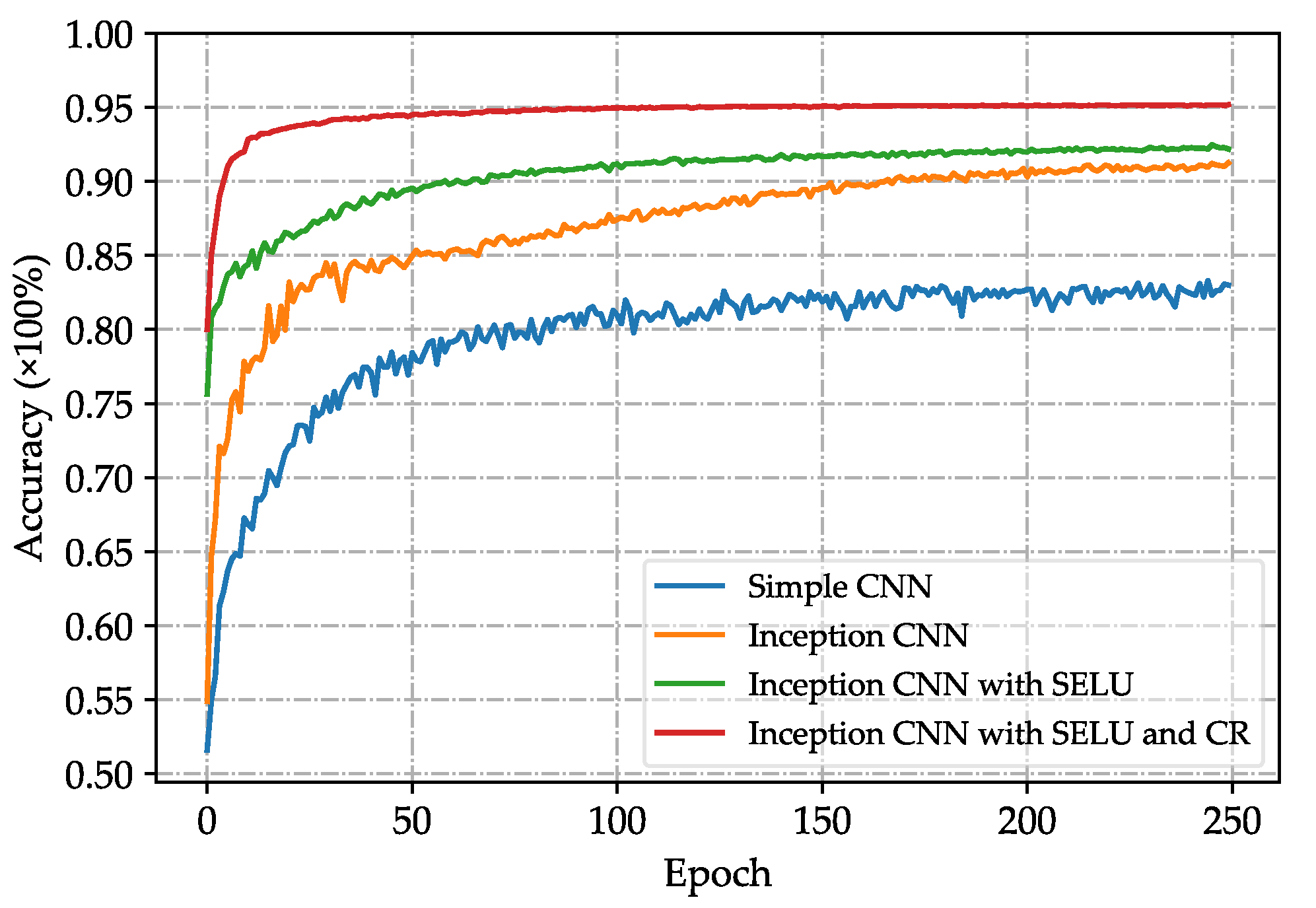
The effectiveness and feasibility of the method are verified by the detection effect and the FDI process. On the data set of this paper, the detection accuracy of Inception-CNN is 95.41%, which improves the prediction accuracy by 17.27% and 12.69% compared with the best-performing non-neural network algorithm and simple BP neural networks tested in the paper, respectively.

In addition, this paper constructs the training data set and validation data set of the signal-based sensor FDI method through the Monte Carlo simulation method, which solves the problem wherein the experiment cannot be carried out due to insufficient fault data.

The sensor fault detection method based on Inception-CNN proposed in this paper is a data-driven algorithm. Its accuracy and applicability are positively related to the quality of the data. Thus, in the future, this method can be combined with the mechanism study of the engine to improve the algorithm’s performance through higher-quality data. In addition, the research content of this paper can be combined with the research on the safety control strategy of aero-engines based on sensor value judgment. Taking the research [38] of Cao et al. as an example, if FDI is used as the front module of the safety protection control module in the control loop, the possibility of control strategy failure due to sensor failure can be reduced, and the robustness of the system can be improved.