1. Introduction
Lagrangian points (LPs) have received great interest in the last few decades. LPs represent equilibrium positions in the three-body dynamics, and a spacecraft at an LP remains locked in the reference frame (RF) which rotates with the two primaries (e.g., Sun and Earth or Earth and Moon), maintaining a fixed position [
1]. In addition to these peculiar dynamical characteristics, these positions offer highly advantageous strategic locations for both logistic purposes and the study and analysis of deep space [
2,
3,
4,
5,
6,
7]. For these reasons, the scientific community is showing great interest in visiting LPs and, in the near future, numerous space missions are planned towards these points.
Among other initiatives, the European Space Agency is planning a mission [
8] (formerly known as LAGRANGE) with two spacecraft in Sun-Earth L1 and L5 for observation and monitoring of interplanetary space and solar activity, and the PLATO mission [
9], in Sun-Earth L2 (SEL2). In addition to being targets of specific missions, LPs could also be used as departure points for interplanetary missions. For instance, a recent contribution [
10] showed how departures from either Sun-Earth L4 or Sun-Earth L5 might be extremely favorable for missions to near-earth asteroids (NEAs) that have small minimum orbit intersection distance (MOID), in particular when the target asteroid passes relatively close to the Earth.
In a similar way, the future Lunar Orbital Platform Gateway (LOP-G; formerly named Deep Space Gateway—DSG) is a joint effort led by NASA, in collaboration with CSA, ESA, and JAXA, in order to place a platform close to the Moon, on a stable orbit around, though quite far from, Earth-Moon L2 (EML2). This orbiting platform will be used to greatly simplify some deep space operations, produce a more practical handling of lunar resources, and serve as a supply point for spacecraft, such as Deep Space Transport, moving to and from distant destinations [
11,
12,
13]. NASA published a reference trajectory in the full ephemeris model for a 15-year-long positioning [
14] of the LOP-G. The selected orbit is a southern L2 near rectilinear halo orbit (NRHO) with 9:2 lunar synodic resonance, which minimizes the required station-keeping maneuvers while eliminating eclipses almost completely.
Very small propulsive requirements ( below 100 m/s and often even below 10 m/s) are needed to escape from LPs on low energy trajectories with final C3 () below 0.5 (km/s); these values are suitable, for instance, for missions to NEAs. These kinds of trajectories are the focus of the present paper, which aims at an initial evaluation of escape from SEL2 and EML2 for an electric propulsion (EP) spacecraft.
The optimization of EP escape trajectories is here carried out with an indirect method, which is based on the theory of optimal control and transforms the propellant minimization problem into a multipoint boundary value problem (BVP). The BVP is solved with an iterative single-shooting procedure based on Newton’s method. High-accuracy results were sought. The dynamic model considers four-body gravitation (spacecraft, subject to Earth, Moon, and Sun gravity), JPL ephemeris for the position of the bodies, and solar radiation pressure (SRP). It also includes an 8 × 8 spherical harmonic model for Earth [
15,
16], even though its effect is negligible as no close passage occurs; the harmonic model for the Moon is here neglected but can be easily implemented if needed.
Indirect methods are computationally efficient but may suffer from poor convergence. Techniques to address numerical issues and to find proper tentative solutions are here introduced. The present analysis considers escapes from L2 and does not impose a constraint on the escape velocity direction. Analysis and results are to be transitioned in future studies on escape trajectories for specific missions. A proper tentative solution is needed, and the use of partial solutions and/or solutions of simpler problems is often an effective means to find such tentative solutions [
17]. The solutions obtained here are suitable as tentative guesses for escape from orbits with practical uses, such as NRHOs, and linked to the analysis of the interplanetary phase for the joint optimization of escape and interplanetary transfer to the selected interplanetary destination [
18].
In the recent literature, Ref. [
19] considered evasion from SEL2 in the circular restricted three-body problem. Direct escape was compared to trajectories with Earth gravity assist; impulsive maneuvers were first considered and then extended to EP, using direct collocation and a nonlinear programming optimization scheme. The analysis is here extended to take orbit eccentricity and Moon gravity into account. In the Earth-Moon system, access to LPs was analyzed in Ref. [
20], but the emphasis was not on EP escape trajectories. Impulsive escape trajectories from EML2 were analyzed in Ref. [
21] in the Sun-Earth-Moon bi-circular restricted four-body problem, either for direct escape or via Earth swing-by; the Sun gravitational perturbation and the relative Moon angular position were both considered. Here the analysis is extended by implementing the use of EP, the JPL’s DE430 ephemeris, and a higher fidelity model for non-assisted EML2 escapes. Results will highlight the influence that the most relevant parameters (e.g., time of flight, positions of the perturbing bodies with respect to each other and to the spacecraft) have on propulsive requirements and characteristics of the optimal escape trajectories.
Section 2 introduces the dynamic model with a detailed analysis of the relevant perturbations taken into consideration.
Section 3 describes how the optimal control problem is developed and implemented.
Section 4 and
Section 5 show the optimal trajectories obtained for departures, respectively, from SEL2 and EML2; both sections include subsections resulting from trajectories obtained with different boundary conditions.
Section 6 provides examples of applications of the results. Finally,
Section 7 presents the paper’s conclusions.
2. Dynamic Model
The dynamic model considers a point-mass spacecraft with variable mass. The problem state variables are position
r, velocity
V, and mass,
m, of the spacecraft, and are ruled by the following differential equations:
where
is the spherical Earth gravitational acceleration,
is the perturbing acceleration due to Earth’s non-sphericity,
is the perturbing acceleration due to Moon (lunar) and Sun (solar) gravity (i.e., lunisolar effect), and
is the perturbation due to SRP. The trajectory is controlled by the thrust vector
T. The available power and thrust are inversely proportional to the squared distance from the Sun, assuming efficiency,
, and effective exhaust velocity,
c, as constants—
—where
and
are the values at 1 AU and
is expressed in AU.
The Earth Mean Equator and Equinox of Epoch J2000 frame (i.e., EME2000) is adopted (
Figure 1);
I,
J,
K are unit vectors along the reference axes of EME2000. Precession and nutation are neglected. Right ascension
and declination
are introduced along with the radius magnitude
r to write the position vector as
. The topocentric RF, identified by unit vectors
𝚤 (radial),
𝚥 (eastward), and
k (northward) is introduced. The unit vectors are defined by the following:
The position vector in the topocentric frame is
and the velocity vector is expressed as
, with
u,
v, and
w as the radial, eastward, and northward components, respectively. The seven scalar state equations are easily derived as
Boundary conditions contain initial values of position (
,
,
), velocity (
,
,
), and mass (
), and final values of
. Constraints on either the final value of
or the final time may be introduced. No constraint is imposed on the final value of the terrestrial longitude and latitude. The final mass is maximized. The perturbation due to Earth’s harmonic potential was already present in the dynamical model and has been maintained, even though it has negligible influence on results and speed of calculations—it is described in Refs. [
15,
16]; details are here omitted for the sake of conciseness. Results show that SRP has a negligible influence on performance for the present study, causing variations of the final mass of a few grams. Nevertheless, the SRP perturbation is included in the integration (for further references, please refer to Ref. [
15]), but it is not further analyzed in the results.
Lunisolar Effect
DE430 JPL ephemerides [
22] are used to retrieve Moon (subscript
ℓ) and Sun (subscript
s) positions. If subscript
b is used to indicate a generic body, its position vector
is given in rectangular coordinates
,
,
with respect to the Earth in the international celestial reference frame (ICRF), i.e.,
. The small differences between ICRF and EME2000 are neglected, and the latter is used in the present analysis. The gravitational perturbation caused by the body, which has gravitational parameter
and position vector with respect to the Earth
, is obtained as the difference of the gravitational accelerations on spacecraft (
) and Earth (
). One has
where
is the spacecraft relative position vector (and
is Earth’s relative position) with respect to the perturbing body. A schematic representation is provided in
Figure 2 below.
The acceleration is projected onto the topocentric frame at epoch to easily obtain the perturbing components. When the perturbing body is very far compared with the Earth–spacecraft distance (i.e., when
, as it happens for the Sun) and coplanarity is assumed, a simple expression of the tangential and radial components of the perturbation can be derived (please refer to Refs. [
15,
16] for further details).
where
and
are, respectively, the tangential and radial unit vectors.
The spacecraft velocity has main components along tangential and radial directions, so these terms can be used to estimate the positive or negative effects of solar perturbation during the escape. Equations (13) and (14) show that it is possible to enclose the perturbation effect dependence on Sun–spacecraft position in the two following proportionality terms:
where
is the angular difference between the Sun and the spacecraft. Energy is increased by the acceleration component along the spacecraft direction. Large positive
tends to be more useful during the initial phase (tangential velocity), whereas large
should be preferred in the final phases, when the velocity tends to the radial direction. Large
occurs when the Sun is in the first (
) or third (
) quadrant in the spacecraft rotating frame, whereas other
combinations may have null or negative influence on the spacecraft energy if the spacecraft is continuously moving outward. The radial acceleration, on the other hand, cannot produce a negative effect (unless the spacecraft is moving towards the Earth) and has a maximum positive influence when the Sun is in between the fourth and first quadrants (
) or in between the second and the third quadrants (
and
). In general, the combined effect of the two solar perturbation components may produce an overall positive effect on the spacecraft energy when the Sun is either close to
or
with respect to the Earth–spacecraft direction.
3. Optimization
The theory of optimal control [
23,
24] is applied to the differential system described above to determine the optimal solution for escape. The final mass is maximized, given the initial state (position, velocity, and mass) and the final distance from the Earth. The final time and/or the final value of
C3 may be added to the boundary conditions. Thrust (magnitude, constrained between 0 and the maximum available value, and direction) is the control variable. Adjoint variables
are coupled to the state differential equations and the Hamiltonian is defined as
. Euler–Lagrange equations provide differential equations for the adjoint variables; they are presented in
Appendix A, and additional details can be found in Ref. [
15]. The Hamiltonian must be maximized by the optimal controls, i.e., thrust magnitude and direction, in agreement with Pontryagin’s maximum principle (PMP). The thrust
T must be parallel to the adjoint vector
, also named the primer vector. The Hamiltonian is rewritten as
, and is linear with respect to
T; a bang–bang control arises and the thrust must be maximized,
, when the switching function
, while the thrust shall be null
, when
. Singular arcs, usually associated with atmospheric flight, are here excluded.
The handling of thrust discontinuities is one of the main challenges in indirect optimization, because they can create numerical problems in the gradients evaluation. Several techniques have been used to deal with this problem, such as smoothing techniques [
25,
26,
27] or homotopy and continuation approaches [
28,
29]. More recently, new regularization techniques, such as uniform trigonometrization methods [
30] and integrated control regularization methods [
31], have also been introduced to handle thrust discontinuities and other kinds of path constraints.
In this analysis, a different approach is adopted. The switching structure (i.e., a suitable sequence of thrust and coast arcs) is specified a priori, and modified if PMP is violated. The simplest thrust–coast structure is initially assumed and eventually modified when required, according to PMP. Each trajectory is divided into a number of distinct phases equal to the number of thrust and coast arcs specified, thus producing a multipoint boundary value problem. The duration of each j-th phase, , is unknown and subject to optimization. Additional boundary conditions specify that the switching function must be null at the switching points, where the engine is turned on or off. This approach guarantees improved numerical accuracy and convergence speed/robustness compared with the alternative strategy of deciding the thrust level during integration, according to the instantaneous value of the switching function.
The equations are integrated by using a variable-order, variable-step integration scheme based on Adams–Moulton formulas. The achieved numerical accuracy is therefore comparable to the one obtained via high-precision orbital propagators in commercial or open-source software, such as STK or GMAT; as expected for indirect methods, computational times are minimal—below 10 seconds per trajectory on a standard 2.70 GHz CPU laptop—if the initial guesses are within a reasonable error range.
The initial values for some variables, e.g., the adjoint variables, are generally unknown. In order to solve the BVP, a Newton’s scheme is adopted. Tentative values
q are assumed for the unknowns (switching/final times and unknown adjoint initial values) and the error on the boundary conditions is determined after integration. Each
i-th component of
q is perturbed by a small quantity
(e.g.,
) and the variation of the error
is evaluated, again after integration. The unknowns are corrected at each iteration, aiming at nullifying the errors by assuming linear behavior and evaluating numerically the error–gradient matrix
, so that
where
K is a relaxation parameter. Values between 0.01 and 1 are usually suited to obtain convergence.
A suitable tentative guess can be built from simple considerations. Given the initial state, a switching structure with a thrust arc followed by a coasting arc can initially be assumed. The length of the burn can be estimated from the available thrust acceleration, assuming a reasonable (e.g., 50–100 m/s for these cases). The velocity adjoint vector is taken parallel to the spacecraft velocity (energy gain is usually sought), with a magnitude that makes the switching function positive. The position adjoint vector is taken in the radial direction and with magnitude to have a decreasing magnitude of primer vector and switching function. Once a solution for a specific case is found, it can be used as a tentative guess for different scenarios (e.g., departure date, constraints on escape C3, etc.).
The boundary conditions at escape are geocentric. In addition to the final radius, the escape characteristic energy, and therefore C3, may also be specified. It follows that the same geocentric C3 can produce different heliocentric energies based on the escape direction, which is here not constrained. The Results Section will present some observations about the heliocentric escape conditions, but a detailed analysis is left for future studies.
4. Escape Trajectories from Sun-Earth L2
In 2018, the European Space Agency proposed an F-class mission [
32] departing from SEL2, where the spacecraft is carried as a piggyback of the ARIEL or PLATO missions. The spacecraft would remain in L2 for a suitable time and then depart from this point for an interplanetary trajectory; the escape trajectory is analyzed here. According to the preliminary mission specifications, a spacecraft mass of 850 kg is considered. The propulsion system is based on the performance of the ArianeGroup RIT 2X: Power available to the thruster
kW (distance from the Sun
in AU), constant efficiency 0.625, constant specific impulse 3300 s, with the thrust that scales as power.
Departures from the Lagrangian point L2 of the Sun-Earth system are considered. The initial distance from the Earth is the radius of Hill’s sphere, evaluated by supposing that the mass of the smaller primary (Moon with respect to Earth or Earth with respect to Sun) is much smaller than the bigger primary. Velocity is selected to have the same angular velocity of the primaries relative motion. One has
where
is the Sun-Earth distance at epoch
. Quantities are here normalized by using Earth’s ellipsoid major semi-axis
km and the corresponding circular velocity
as reference values, where
km
3/s
2 is Earth’s gravitational parameter. The normalized gravitational parameter of the Earth is equal to one.
The reference departure date is 15 October 2025, when the instantaneous Earth-Moon distance matches its average value of 384,400 km. The analysis time is extended up to the point in which the instantaneous Earth-Moon distance is again at the average value, which happens on 12 November 2025. Five sample cases are of interest, namely one each week, hereinafter referred to as cases 1–5.
SEL2 departures have been analyzed under different constraints. In particular, the distance of escape is always fixed at 3 million km from the Earth, namely beyond Earth’s sphere of influence (SOI), when the combination of gravitational attractions of Earth and Moon becomes negligible compared with the Sun’s one. The first analysis bounds the time to escape at 90 days, while leaving the final energy as a free parameter. Then, escape C3 equal to 0.2 and 0.5 (km/s), with no constraints on the escape time will be considered.
4.1. Sun-Earth L2 Escapes with Constrained Final Time
The solutions for the five departure dates show a common trend during the escape.
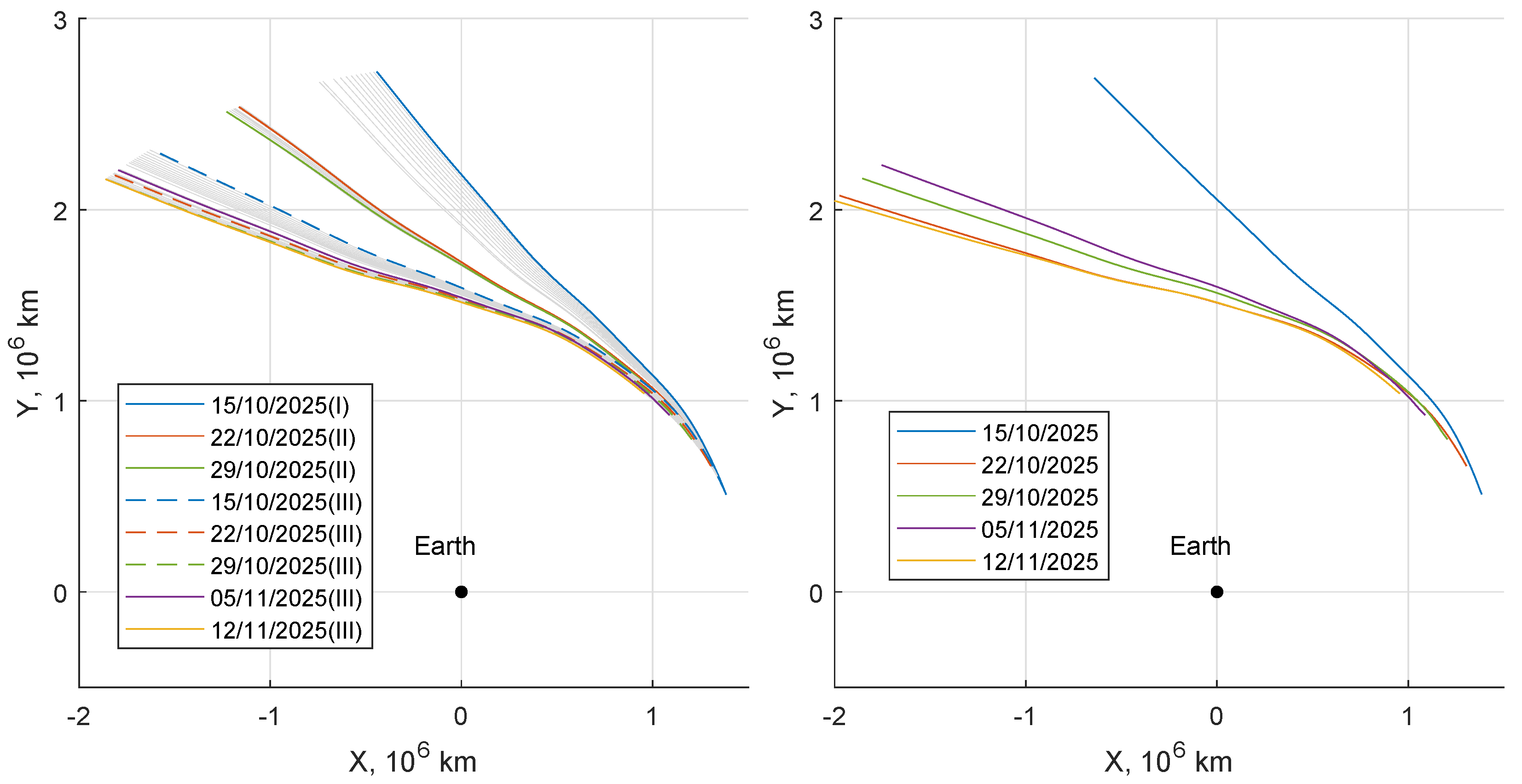
Figure 3 highlights a whole family of solutions (represented by the hundreds of subtle lines) with departures starting from case 1, on 15 October 2025, up to case 5, on 12 November 2025. These selected five cases are henceforth highlighted with specific styles. A family collects solutions that can be found with a continuation approach: There are close similarities, and, at a first approximation, each curve seems simply rotated due to the different departure position. Each trajectory is however different, mainly due to the Moon position during flight, which changes with the departure date.
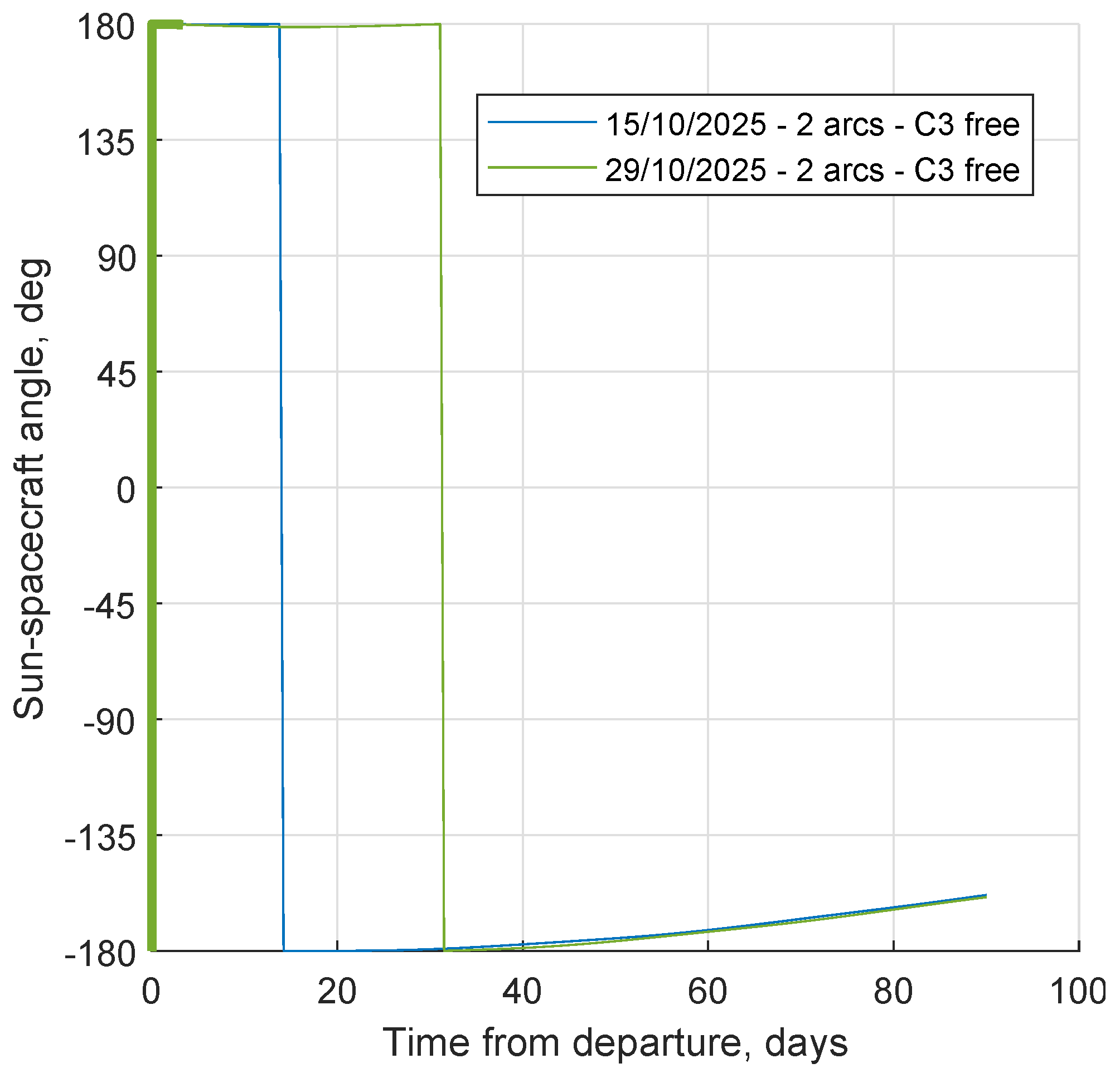
The spacecraft is actually pulled towards the boundary of the SOI by the Sun, which has a large positive overall effect on the orbit energy. Its direction at the beginning and at the end of each selected escape is represented in the lower part of the figure. Thrust is therefore used to achieve a trajectory that maintains the Sun in a favorable position, maximizing the effect of its pull (
close to 180
, see
Figure 4).
Figure 5 shows that for the selected SEL2 escapes the whole energy gain, except for a minor thrust contribution at the beginning, is due to the solar perturbation. Please note that, henceforth, thrust phases are shown as bold lines in those figures that may contain that information.
Thrust is used so that the Sun moves from the second to the third quadrant of the frame that rotates with the spacecraft, where Sun’s gravity acts to increase the orbit energy. The spacecraft remains close to
and/or between
and
in the rotating frame, exploiting both tangential and radial components of Sun’s perturbation. The same trend is shown for different departure dates, with the initial thrust arc adapting to produce the same effects, as shown in
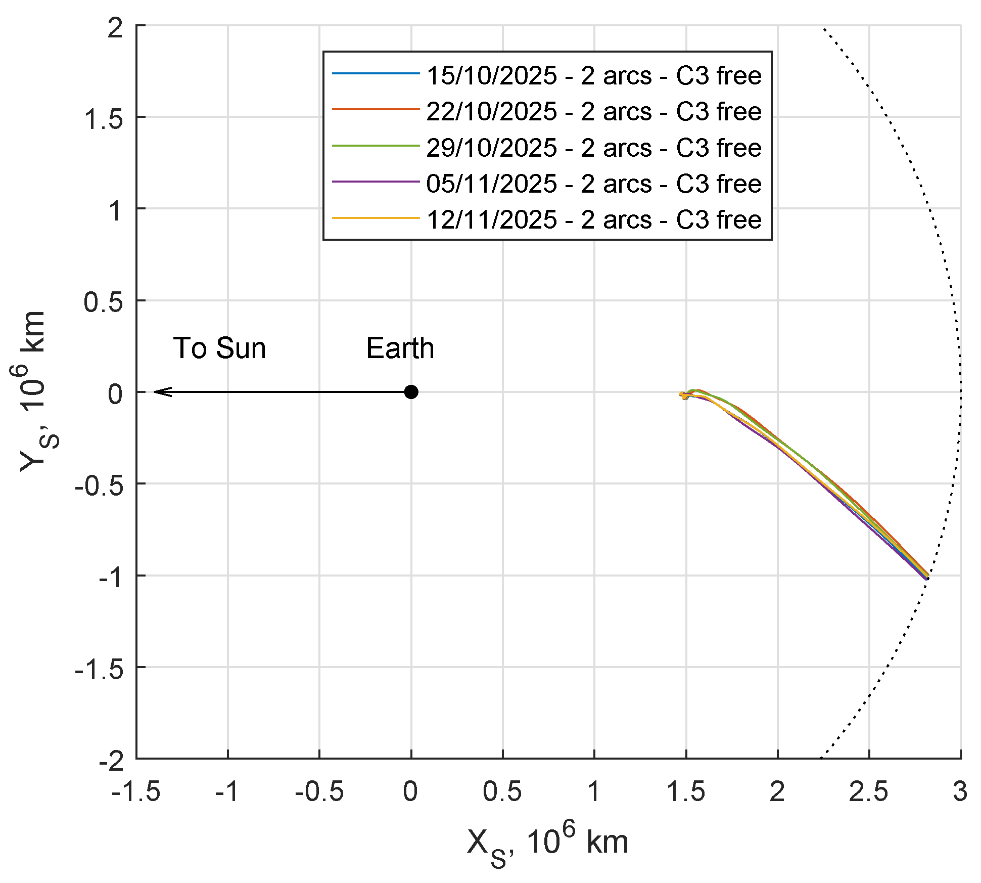
Figure 4. In a Sun-Earth synodic RF centered on Earth (
Figure 6), such trajectories are all located in the fourth quadrant and show evident similarities during the escape.
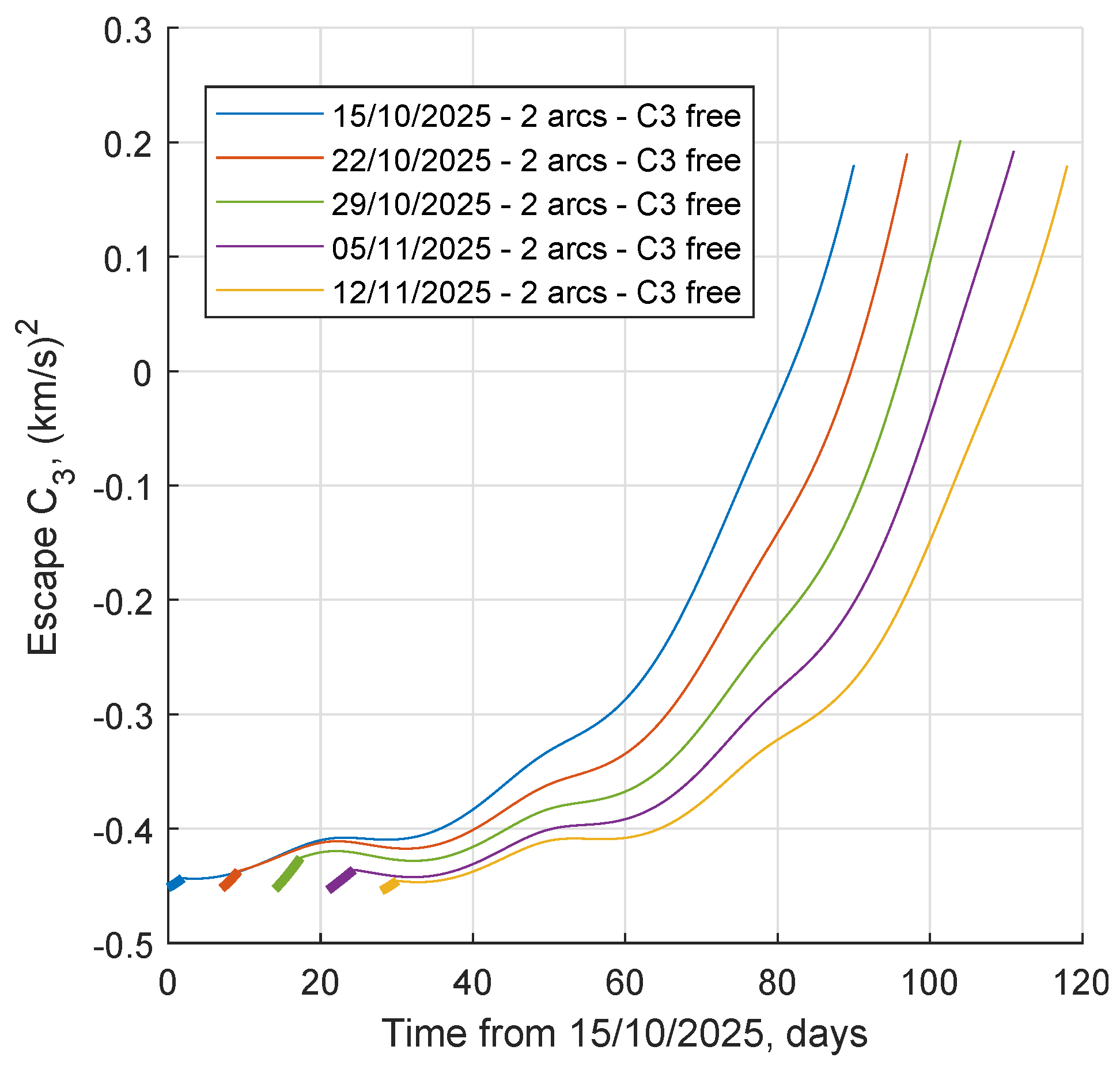
The effects of Moon’s perturbation are shown in
Figure 7, which presents the trend of the propellant requests, and thus the
, to reach an escape in 90 days with free final energy. The reference departure date (15 October 2025) is in the region where
and
C3 values are lowest. The spacecraft is relatively far from the Moon, and Moon’s gravity acts mainly on the Earth. The initial geometry on the reference departure date shows that the Moon reduces the spacecraft’s geocentric energy by pulling the Earth; this perturbation modifies the Sun-Earth–spacecraft geometry so that the Sun’s pull on the spacecraft is increased, and a lower propulsive effort is needed. The opposite happens after half the lunar period. The final value of
C3 depends on the energy gain provided by thrusting and the overall effect of the perturbing bodies, causing oscillations in the trajectory performance.
The effect of Sun’s pull is dominant, and two simple coefficients are defined to assess how much the influence of the solar perturbation is acting favorably on the escape,
and
. The radial and tangential perturbation weights are introduced to evaluate the normalized contributions of solar perturbation along the whole trajectory. The trajectory is split into
n uniform intervals and
and
are evaluated as
For each family of solutions, the are normalized with respect to the longest mission among them. This allowed us to produce a general parameter able to compare those escapes with a different total duration.
The 1/2 coefficient in
is introduced to make
for maximum favorable effect, whereas
corresponds to null effect. The values of
, instead, range between −1 (most unfavorable) and 1 (most favorable).
Figure 8 shows the trend of these coefficients; it is clear that SEL2 escapes exploit mostly the radial perturbation, with slight fluctuations of the tangential perturbation that, however, acts always favorably. Even though they are not an exact measure of solar effect, these coefficients correctly match the actual propellant consumption trend, with minimum propellant requirements in the region between maximum
and
.
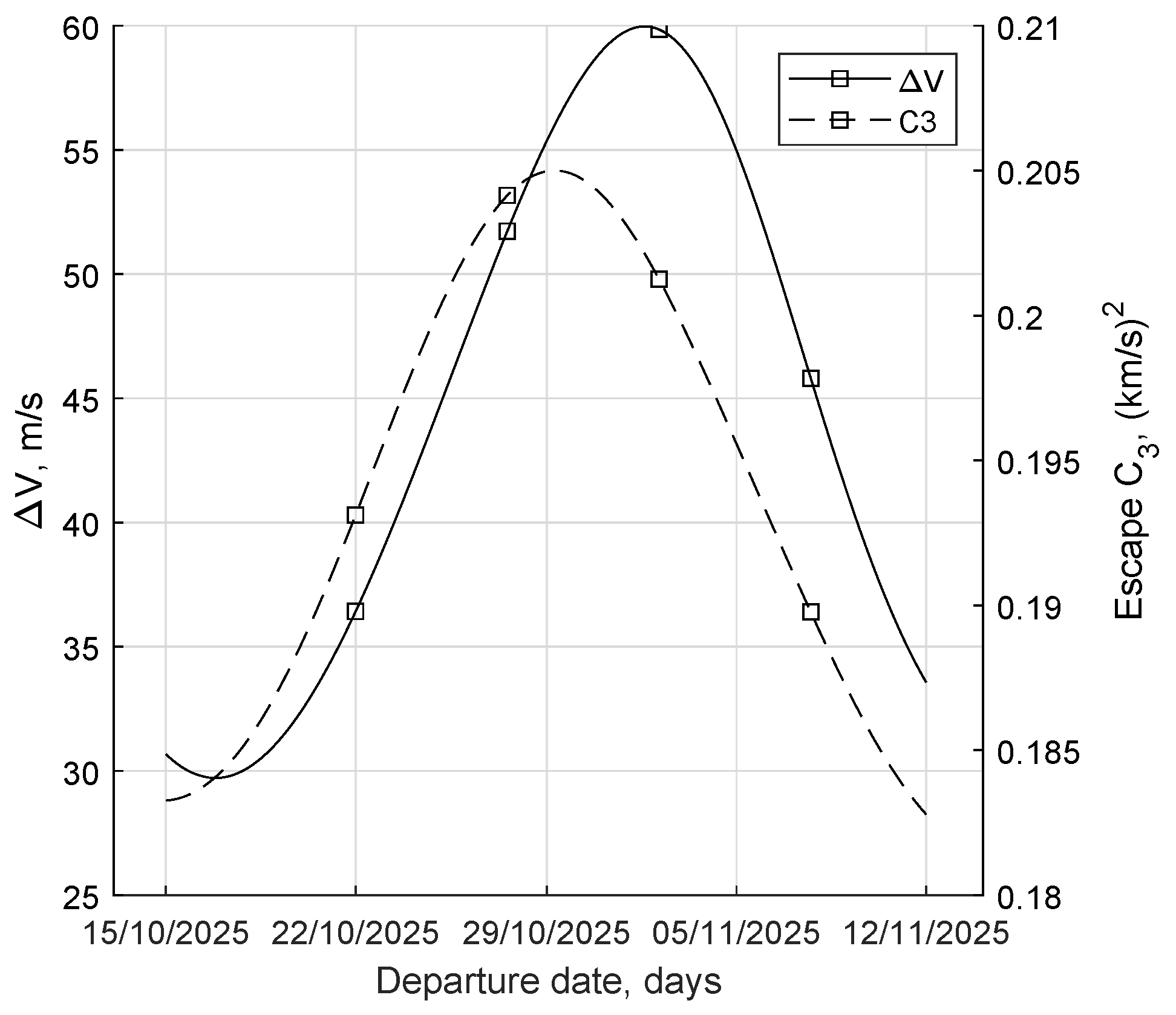
Table 1 compares the performance of the reference cases C = 1–5, depending on the departure date. All the solutions belong to the same family (f = I) and have a 2-phase structure (
p = 2).
4.2. Sun-Earth L2 Escapes with Constrained Final Energy
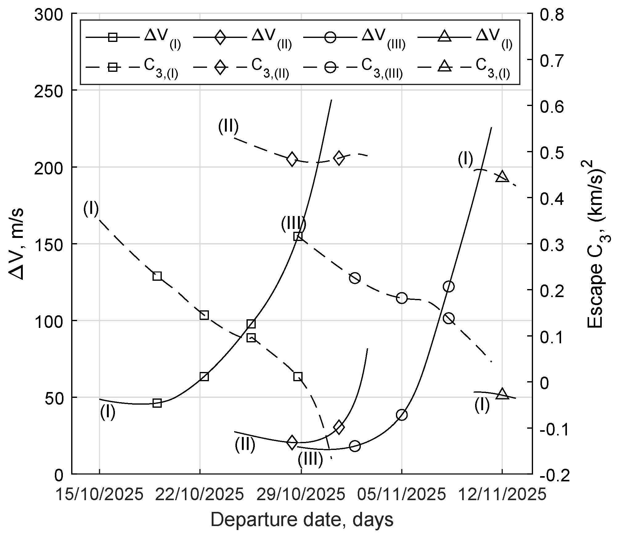
When the escape maneuver is the start of an interplanetary transfer, specific values of escape energy and C3 could be sought. If the final C3 value is constrained, then the escape trajectory is modified to change the overall effect of Sun’s pull. Two case studies have been analyzed, by imposing the final C3 equal to 0.2 and 0.5 (km/s).
Given the high sensitivity of the convergence process to the adjoint variables initial values, both the exploration procedure to generate a family of solutions, and the passage from a solution with the same departure date to a new case with different final conditions, are particularly delicate. Compared with the previous study [
16], various methodologies and techniques have been developed and implemented to guarantee robustness to the method and to automate many of these processes. The case studies solutions at fixed
C3 have been found one-by-one starting from a set of tentative solutions built on user experience (initial thrust aligned with velocity, thrust–coast structure). The other solutions have been found similarly or via an ad hoc continuation method. A gradual variation is imposed, starting from the free final
C3 solution towards the constrained one (or from the lower to the higher constrained final
C3) or using the closest available solution in terms of departure date as a tentative guess. It can happen that a forward search from a certain date and a backward search from a later date do not end up to the same point; therefore, for the same departure date, solutions belonging to different “families” are found.
This bifurcation phenomenon is visible in
Figure 9 (left), which shows that three families of solutions arise from the single family at fixed escape time when solutions are forced to
. On the contrary, all the solutions for
have the same strategy. Analogous considerations are shown in
Figure 10, in which all the trajectories reach the same final
C3 but with different costs and mission durations.
The first family is found for departure between 15 October 2025 and 21 October 2025, with trajectories that tend to be radial and have short trip times. The second family is for departures between 18 October 2025 and 2 November 2025. The third family extends over the whole launch period considered, and has trajectories with a more tangential velocity with respect to the other solutions. This result shows how, for the same departure date, it is possible to pick different strategies according to the specific needs; at the same time, it is clear that the improved code allows the indirect method to find various solutions without falling in the same local minima. In this case, family III is always the better solution for what concerns propellant consumption, but different constraints (C3 value, additional time constraints) may change the scenario.
Figure 11 shows the trend of the spacecraft energy over time. It can be seen that the solution with final
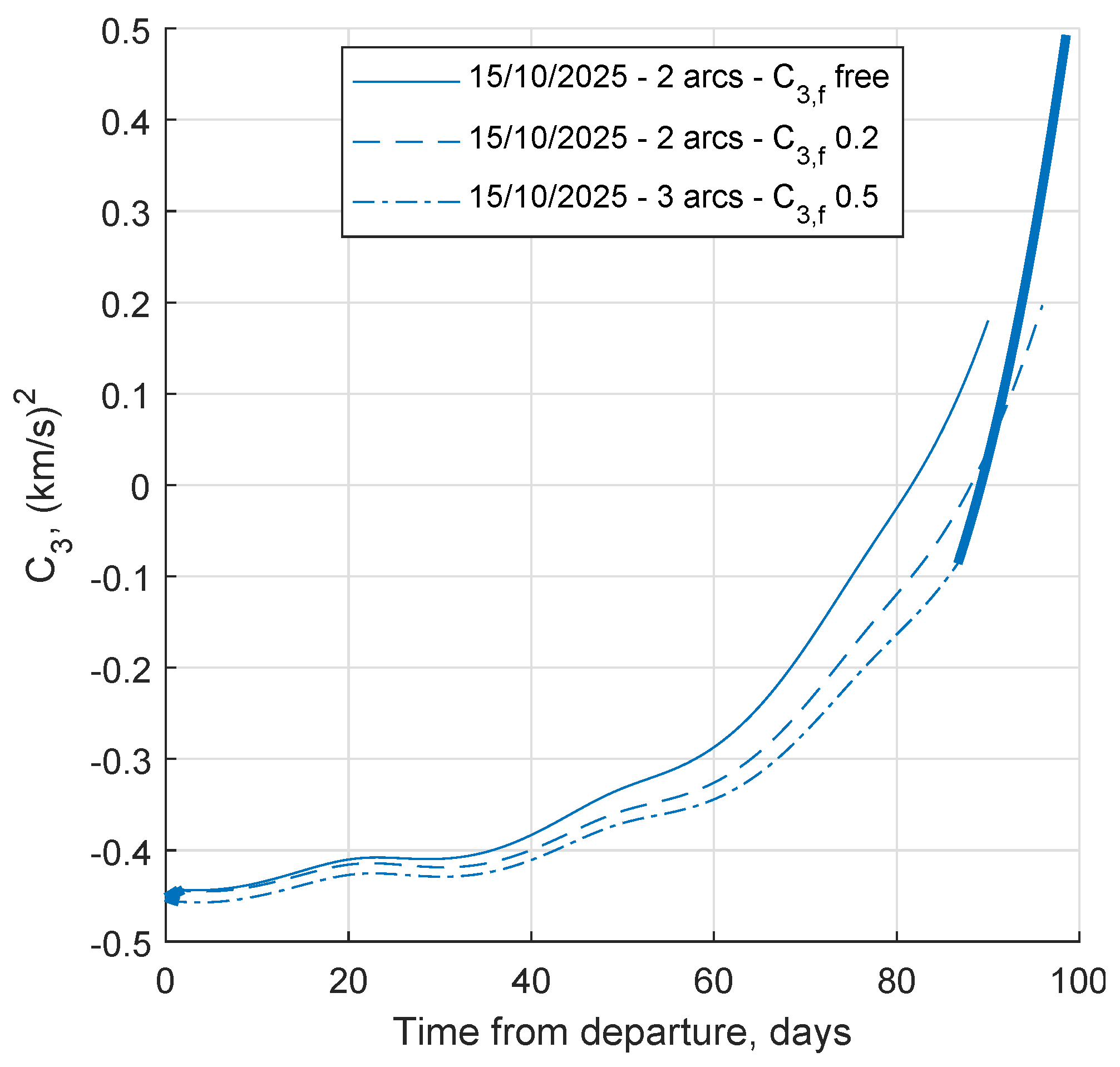
includes an evident second thrust arc (T) after a coast arc (C), for a total of three phases in a T–C–T strategy. In this case, later thrusting is preferred to achieve the desired large final energy, instead of increasing the initial burn duration, in order to maintain an unaltered positive effect of solar perturbation.
Table 2 and
Table 3, instead, show the solutions for the escapes with fixed final energy, while in the lower final energy scenario multiple families of solutions arise, in which some trajectories exploit more consistently the solar perturbation, whereas others use more propellant, the scenario with higher final energy only relies on a second consistent final burn to reach the desired final energy as the only feasible option.
Figure 12 shows the semi-major axes of all these trajectories in the heliocentric ecliptic reference frame, on the left for the lower energy scenario and on the right for the higher one. The integration is extended to 2.5 times the time to escape to show the evolution after the exit from Earth’s SOI; while for the final
(km/s)
case, this operation produces a simple extension of the final coasting phase, in the
(km/s)
scenario, the appearing of a fictitious terminal fourth coasting phase is needed. All the trajectories have similar trends with comparable costs, almost equal use of the solar perturbation and similar final energies. However, as anticipated, the escape directions are different; therefore, the orbital parameters, as shown in
Figure 12, show slightly different trends. It is worth noting that small variations occur after the escape for the residual influence of Earth’s gravity. Nevertheless, departures spaced apart by one lunar month overlap again quite precisely.
5. Escape Trajectories from Earth-Moon L2
The dynamics in the vicinity of EML2 is characterized by a complex gravitational interaction between the Sun, the Earth, and the Moon. Nevertheless, several researches and missions have exploited this region for the numerous strategic and design advantages that it can offer. Indeed, in 2004, the ESA’s Advanced Concepts Team researched the use of Lagrange points as departure and arrival points of space missions, demonstrating that the characteristic orbits nearby of these points are accessible in reasonable times and costs [
20].
Lissajous orbits around EML2 have been used for the Artemis P1 mission in 2010 and Chang’e 5-T1 in 2014. The recent Chang’e 4 mission used a halo orbit around EML2 for its relay satellite, Queqiao, which is positioned at EML2 since 2018 for signal-and-sunlight eclipses avoidance. The NASA’s Exploration Campaign in 2018 assessed that the Artemis program would include the positioning of an outpost in the vicinity of EML2, the LOP-G, in a Southern Synodic 9:2 NRHO, that will serve to enable future deep space exploration missions. By the middle of 2022, the NASA Artemis 1 mission, formerly Exploration Mission 1, is expected to take place. NASA selected 13 secondary payloads to be transported in the new SLS Block 1, among which there will be EQUULEUS, a 6U Cubesat proposed by JAXA and the University of Tokyo [
33]. Its primary goal is a low-energy trajectory control experiment near EML2; its mission and scientific objectives are discussed in Ref. [
34].
These important missions and programs simultaneously show the high scientific interest and the complexities in the use of such L2 points. The proposed analysis implements direct escapes from EML2 and disregards the complexities that would derive from the inclusion of NRHOs or Lissajous orbits as departure points, which will be subject of future research. As per the SEL2 case, the propulsion system has the same values for power and efficiency, but the specific impulse is imposed constant at 2000 s, like in a typical, current Hall thruster.
The same specific five departure times in a lunar synodic period of the previous section are again considered to explore the effect of the relative position of the Moon and the Sun on the escape maneuver. The first (15 October 2025) and last (12 November 2025) departures happen at times with the nominal Moon’s mean orbital radius; a perturbed Moon orbit is considered so the positions in EME2000 are slightly different. The linearized L2 distance is again used to define the spacecraft initial position. One has
The final radius is fixed at 3 million km, beyond Earth’s SOI boundary. Like in the SEL2 departure analysis, three scenarios are considered: the first with a fixed time to escape and a free final energy, and other two with escape C3 fixed at a lower (0.2 (km/s)) and higher (0.5 (km/s)) value with free time to escape.
5.1. Earth-Moon L2 Escapes with Constrained Final Time
In similarity to the escape from SEL2, single burn trajectories are initially sought; these trajectories are characterized by a first thrust (T) arc followed by a coast (C) arc.
Figure 13 shows the manifold of departure trajectories for the selected dates. Those trajectories exploiting a second burn are distinguished by a small dot at the arc end. The first (15 October 2025) and last (12 November 2025) departures, i.e., cases 1 and 5, have slightly different initial positions in EME2000 and the Sun relative angle has a difference of about
. Nonetheless, the two solutions are similar with a difference in spacecraft final angular positions close to the
between Sun positions. When additional departure dates are considered, three families of solutions can be distinguished (see also
Figure 14). Due to the greater dynamic complexity of the Earth-Moon system, even the trajectories with fixed final time and free final energy split into several families.
Table 4 shows the performance for the selected departure dates in each family, and
Figure 15 shows some of them to highlight the differences.
In particular, by observing the same trajectories in the Sun-Earth synodic reference frame centered on Earth (
Figure 16), three escape trends arise. Cases 1, 2, and 3 of family I occupy the first and fourth quadrants, favorably exploiting the radial component of Sun’s perturbation in the final part of the escape, in accordance with
Figure 15. The spacecraft always shows terminal
close to
, while case 2 exploits a short second burn to align the final leg of the trajectory, the late departure of case 3 forces a longer initial burn to achieve a similar result (
Figure 16, right). The specular scenario, for cases 3 and 4 of family III, sees escape points on the L1 side (i.e., between Earth and Sun, see
Figure 4). These trajectories occupy the second and third quadrants in the rotating reference frame, tending to null
, which, again, implies favorable radial perturbation. The single trajectory in the second quadrant, case 3 family II, exploits more substantially the tangential component with an escape tending to
. The last trajectory, case 5, repeats the trend of family I solutions, being in particular very close, as expected, to the solution departing a lunar synodic month earlier, even though the different position of the Sun affects the trajectory details.
The reference departure date has a T–C escape strategy with low propellant consumption, which corresponds to a positive use of both the tangential and radial solar perturbation as seen from the evolution of the relative angle between the spacecraft and the Sun. The same switching structure does not respect PMP for the second departure date. In this case, the switching function becomes negative during the thrust arc, suggesting that the thruster should be turned off. The switching structure is modified in agreement with this behavior and a four-arc trajectory, T–C–T–C, is adopted. The two-burn solution respects PMP and is therefore optimal; the propellant consumption is correspondingly reduced with a significant improvement. Case study 3 has solutions pertaining to three different families, and by analyzing the Sun–spacecraft relative angle from family I to family III, one can notice that increasingly improved strategies can be implemented. The first family shows a very high propellant usage to contrast the long period (roughly, between 15 and 50 days since departure) in which the spacecraft is at a null or negative configuration for the tangential perturbation. The second family has a similar condition but has favorable radial perturbations, leading to a wider trajectory at a lower cost. The third family, which spans also to the fourth departure date, is the most favorable one, and it exploits a consistently positive tangential perturbation. Indeed, even if cases 3 and 4 from family III have departures separated by
, they tend to both end at
. The same considerations are highlighted in
Figure 17.
It is noteworthy that the second family of solutions has a very low propellant consumption with a very high free final energy, implying that constrained final energy solutions, especially the ones fixed at lower values, will have to reduce somehow the spacecraft energy to achieve the desired boundary conditions. The same applies to part of family III solution and to case 5 (family I).
5.2. Earth-Moon L2 Escapes with Constrained Final Energy
The trajectories with fixed final energy have been calculated with the same strategies implemented for the SEL2 case. The complexities due to the proximity of the Moon and the perturbations of the third body divide more evidently the families of solutions compared to the cases with free final energy.
Figure 18 shows on the left all the solutions found for the fixed low energy scenario, while on the right those for
(km/s)
. The families still have many solutions within them, but most of them tend to overlap in their final phase when the final energy is fixed.
Many T–C solutions of the free
C3 case assume the two-burn T–C–T–C structure when constrained to
(km/s)
, especially those belonging to the second family. Moreover, a peculiarity to be observed, clearly shown in the corresponding
Table 5 and
Table 6, is that low-energy and high-energy fixed solutions, for selected studies, tend to invert the optimal thrust structure from 2 to 4 phases and vice versa.
Figure 19 shows that solutions group themselves towards favorable values of the solar perturbation. For the
(km/s)
scenario on the left, some trajectories are shown; case 1 and case 2, from the family I, have high positive values of the solar tangential perturbation, while cases 3 and 4 from family III overlap towards the same scenario, in the opposite heliocentric direction. The corresponding family II solution of case 3, which is a two-burn trajectory, exploits more consistently the radial component and uses more propellant to achieve the escape. The
(km/s)
case, on the other hand, has trajectories that move towards positive influences of the tangential solar perturbation, with cases 1, 2, and 5 that favor the Sun in the third quadrant and cases 3 and 4 in the first quadrant. Only case 2, depicted in
Figure 18 (right), which departs 90
later than case 1 but converges to the same final point, needs to perform a longer burn at the beginning to align the outward trajectory to the correct direction.
Figure 20 shows two sample cases, 2 and 3, selected to show low- and high-energy trajectories that must either increase or decrease the energy to achieve the fixed energy counterparts. In particular, case 2 from the free energy scenario has a very low final energy, whereas case 3 has a very high one. The four-arc solution for case 2 slightly reduces its duration while increasing the first thrust phase to comply with the final energy increase and keep similar
during the escape. This action eliminates the second burn making it a T–C trajectory. When forced to have the higher final energy, the optimal strategy keeps reducing the overall duration to escape, while increasing the thrust phase length; indeed, the solution forces the relative angle to stay in the third quadrant between
and
, where the solar perturbation acts more favorably.
With an opposite behavior, the single burn solution in the scenario with free final energy for case 3 has to reduce its overall energy to achieve the required lower C3. This increases the overall length of the trajectory with a strong reduction in the first burn phase, showing that the optimal strategy relies mainly on the solar perturbation to achieve the desired energy. Indeed, the majority of the escape, after the initial 30 days, remains in a region in which the Sun perturbation has a negative effect, retarding the energy increase.
6. Applications
The results obtained in this article represent a preliminary approach to the indirect optimization of escape trajectories from Lagrangian points. On the one hand, they can be used as tentative solutions for the indirect optimization of escape transfers from practical orbits around/in the vicinity of Lagrangian points. On the other hand, these escape transfers can be coupled to the analysis of interplanetary legs for the design of missions aimed at near-earth asteroids.
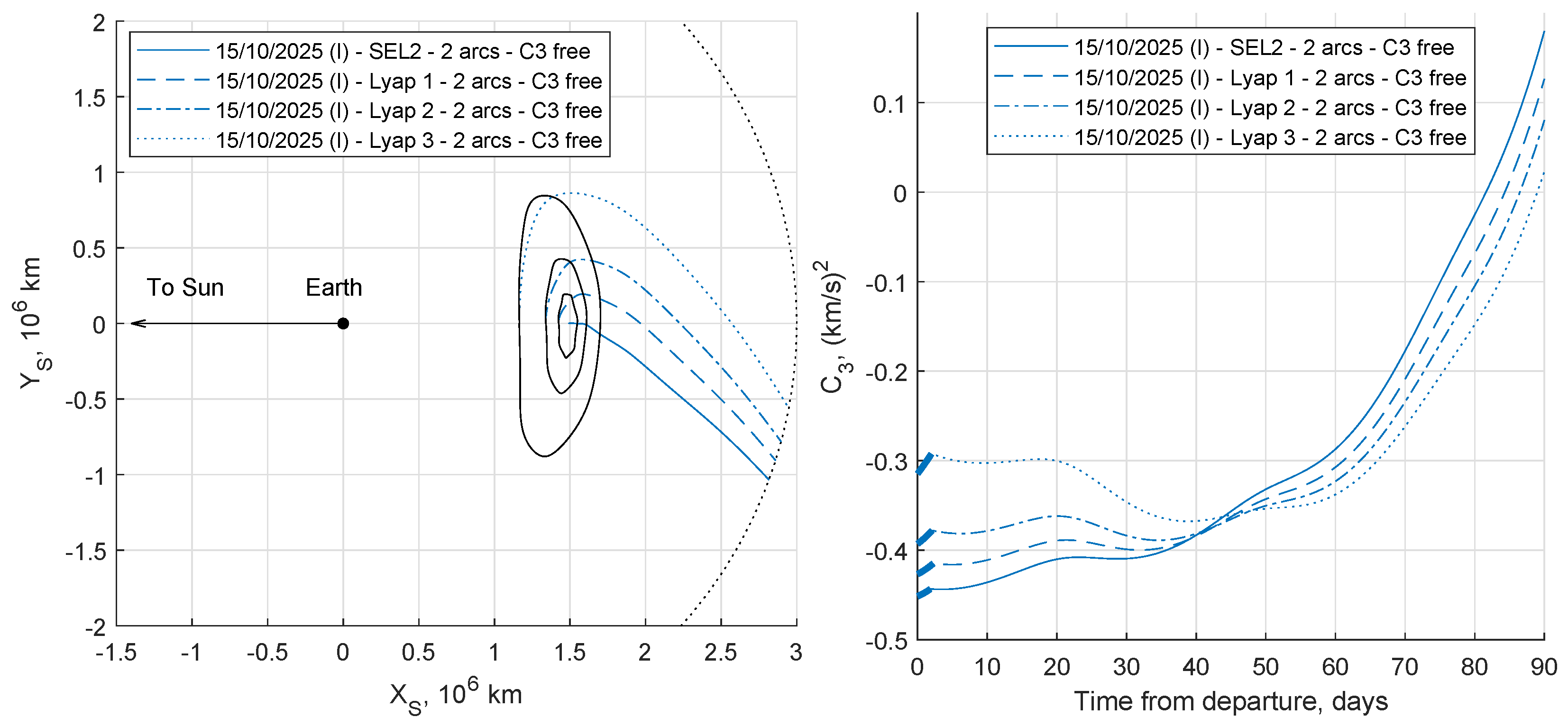
A complete analysis of escape transfers for different orbits around SEL2 and EML2, considering the influence of orbit characteristics, departure point and date, etc., is beyond the scope of the present article. Only high-fidelity Lyapunov orbits around SEL2 are considered as examples. Departure occurs on October 15 2025, from the orbit intersection with the Sun-Earth L2 line, i.e., the
x-axis of the Sun-Earth synodic frame, (between Earth and L2) and 90-day escape transfers with free
C3 are considered. The initial orbits are characterized by their Jacobi constant and start from the
x-axis at about
km,
km, and
km from L2. The solution starting from L2 is used as a tentative solution for departures from Lyapunov orbits and convergence is readily obtained. It is worth noting that the new solutions can, in turn, be used as tentative guesses for other studies (e.g., for the optimization of departure point and/or escape duration).
Table 7 and
Figure 21 compare the escape trajectories from L2 and from the three Lyapunov orbits. The escape transfers show similar propulsive requirements. Escape
C3 tends to be smaller for the larger Lyapunov orbits; this value is however sensibly influenced by the escape duration and different control structures (e.g., a second thrust arc) could eventually become optimal for constrained
C3 values.
The preliminary design of interplanetary trajectories usually starts from the patched-conic approximation. The analysis of escape maneuvers and heliocentric leg are often treated separately at an initial state, and the results are then coupled for a high-fidelity analysis of the complete transfers. This approach was, for instance, used to design the ARRM mission [
18,
35]. In a similar way, the results for the L2 escape obtained in this article can be useful to design interplanetary transfers. Only the 90-day escape from SEL2 with free
C3 and departure on 15 October 2025, is again taken as an example. The small
C3 value suggests that this trajectory can be fit for transfers to NEAs and a set of 75 asteroids considered in previous works [
36,
37] is explored. The escape direction has a specific orientation in the Sun-Earth system (see
Figure 6), which should be suited to reach only the targets that require a similar orbit correction at the selected departure.
The interplanetary leg with two-body dynamics is optimized with different initial conditions to highlight the effect of the actual escape maneuver on the overall performance. Departure from Earth’s position with C3 = 0 (km/s) on 13 January 2026 (i.e., 15 October 2025, +90 days) is assumed as the reference trajectory. The length of the heliocentric transfer to rendezvous with the asteroid is 3 years. The reference solutions are compared to trajectories with departure from the actual heliocentric position and velocity corresponding to the 90-day escape trajectory departing 15 October 2025.
In this example, escape from L2 improves the reference trajectory for 21 out of 75 available targets. Propellant budget comparison for these solutions is shown in
Table 8, ordered by percentage propellant saving. Note that 8 out of the first 10 asteroids have perihelion in the first quadrant, where the perihelion of the heliocentric orbit at escape lies; the required change in orbital elements is reduced, explaining the saving. The optimal rendezvous transfer is also influenced by a phasing constraint, which may require different orbit adjustments; therefore, this general observation has exceptions.
7. Conclusions
An indirect method has been used for the optimization of EP escape trajectories from either Sun-Earth or Earth-Moon L2. Even in the presence of complex dynamics and nonlinear effects, the method proves to be fast and reliable, thanks to the peculiar treatment of the thrust magnitude. The complexity of motion dynamics makes convergence difficult and causes the existence of local optima. The techniques to obtain converged solutions introduced in this article allow one to efficiently explore the solution space and identify local and global minima of the propellant consumption.
Escape from Sun-Earth L2 is relatively simple, as proper selection of time of flight and departure date can guarantee suitable escape conditions with extremely low propulsive requirements. Escape from Earth-Moon L2 shows the complex interaction that the relative positions of the Moon and the Sun produce on the escape trajectory. On the one hand, the departure date determines the direction of the escape hyperbola; on the other hand, it influences the switching structure as the spacecraft tries to maximize the effect of solar gravity. Privileged escape directions are easily recognized.
The results obtained in this paper offer a good understanding of the main driving effects that characterize escape trajectories from L2. This analysis provides the basis for consideration of different departure conditions. Departure from Lyapunov orbits is straightforward using escape trajectories from L2 as tentative guess. Extension to other cases—such as those that correspond to an NRHO in the Earth-Moon system or a Lissajous orbit around Sun-Earth L2—can then be pursued using continuation approaches to modify the initial orbit.
Indirect optimization is computationally fast and escape trajectories can be rapidly evaluated to build a database of escape conditions/cost. These results can in turn be coupled to the optimization of the heliocentric leg for the preliminary design of interplanetary missions, providing a more accurate evaluation of the propulsive requirements.


