
Flight Speed Evaluation Using a Special Multi-Element High-Speed Temperature Probe


Department of Fluid Dynamics and Thermodynamics, Faculty of Mechanical Engineering, Czech Technical University in Prague, 160 00 Prague, Czech Republic
Aerospace 2022, 9(4), 185; https://doi.org/10.3390/aerospace9040185
Submission received: 15 February 2022
/
Revised: 17 March 2022
/
Accepted: 30 March 2022
/
Published: 31 March 2022
(This article belongs to the Collection Avionic Systems)
Abstract
:In the context of aircraft aerodynamics, the compressibility of air flowing around the aircraft must always be considered. This fact brings with it one inconvenience: to evaluate the velocity of the flowing air (airspeed), it is necessary to know its temperature as well. Unfortunately, direct measurement of the temperature of air flowing at high speed (usually at Ma > 0.3) is practically impossible without knowledge of its velocity. Thus, there are two unknown quantities in the problem that depend on each other. The solution is achieved by a method that uses temperature probes composed of multiple sensors with different properties (different recovery factors). The comparison of rendered temperatures subsequently allows the elimination of the necessary knowledge of static temperature and the evaluation of velocity. In this paper, one of such probes is described together with its thermodynamic properties and possible applications.
1. Introduction
The world has accelerated incredibly in the last 100 years and is accelerating all the time. Whether this is good or not is a rather philosophical question and is not the focus of this article. However, what is important in our field is the fact that the range of fluid velocities whose flow field we would need to describe for a variety of reasons is constantly increasing. The maximum achievable speeds of vehicles or the performance of various turbo machines are increasing. We accepted nature’s challenge of a race against the speed of sound, and in 1947, with the Bell X-1, we won [1]. We are flying into space, building space stations, and preparing for interplanetary flights. All of these activities moving humanity forward have at least one common denominator, and that is the fact that, at the speeds at which our present flying machines move, the compressibility of the fluids in which they move, or which pass through their propulsion units, can no longer be neglected. Other technical applications where this is the case are also numerous, and each of them would certainly be sufficient to warrant a separate publication.
Let us now move on to the heart of the matter, which is related to the possibility of local measurement of the velocity and temperature in the flow field of fluids for which, due to high pressure changes, their compressibility cannot be neglected. The present problem, which was also the motivation for the scientific work largely described in this paper, is that the velocity and temperature of a compressible fluid flow are interdependent, and thus one or the other cannot be measured. In other words, if we were to use a temperature probe placed in a stream of compressible fluid to evaluate the temperature of that fluid, we would also need to know its velocity. Yes, we have velocity probes. However, if we wanted to measure the velocity of a fluid, for example, with pressure probes, we would also need to know its temperature. One solution to this impasse is to use multi-element temperature probes, which are described later in this paper.
Measurement of the flow velocity of compressible fluids using temperature probes, specifically thermocouples, is a well-known method. It was described, for example, by Ishibashi and Morioka in their 2009 [2] and 2012 [3] papers. The method here is named RTA (Recovery Temperature Anemometry) and, as the name suggests, uses a temperature probe with a given recovery factor (described below) to measure the fluid flow velocity. The advantage of the method is the miniature size of the thermocouple node and thus the possibility of placing the probe very close to the wall and measuring inside the velocity boundary layer. Another advantage is the generally low directional sensitivity of the probes that work on this principle. However, the disadvantage is the aforementioned number of unknowns, i.e., the fluid flow velocity and temperature. Ishibashi and Morioka measured the velocity profiles of the air flow behind a precision nozzle made with the ISO 9300 standard cited in the article. They assumed isentropic flow due to the precision nozzle. Therefore, they determined the air temperature behind the nozzle by measuring the total temperature and static pressure upstream the nozzle and pressure downstream the nozzle according to the following equation:
where represents Poisson’s constant (adiabatic power), using for air. Thus, this assumption eliminated one unknown, namely, static temperature, and allowed the velocity, and consequently the Mach number, to be evaluated. However, this step limits the applicability of the method to cases where the temperature can be indirectly determined.
A method that does not require explicit knowledge of the temperature of the flowing fluid is described later in this paper. The described method has been named DRTA (Double-sensor Recovery Temperature Anemometry). Schmirler and Krubner provided a more detailed explanation of the idea and the proposal for the probe design [4]. In summary, the problem can be described as follows.
Let us consider one stagnation point on the front side of the considered temperature probe. Then, it can be expected that the fluid stream is completely decelerated at that point and that the temperature is equal to the stagnation temperature . However, for temperature probes of realistic dimensions, the average temperature of the temperature-sensitive element is also affected by points where only a partial current deceleration occurs, and the resulting temperature is not equal to , but equal to a kind of recovery temperature of the whole probe . That temperature then lies somewhere between the stagnation temperature and the static temperature . The static temperature is sometimes called the temperature of an undisturbed stream of the fluid and is referred to as . The following equation can then be used to determine the recovery temperature of the probe:
where is the above-mentioned temperature of the undisturbed stream, is its velocity, and is the isobaric specific heat capacity of the flowing gas. The probe recovery factor plays an essential role here. For the case where the flowing gas can be described by the ideal gas model, i.e., where can be considered as a constant depending on the specific gas constant and the adiabatic power only such that
it is possible, together with the definition of the Mach number, to rewrite Equation (2) as follows:
Let us assume that the temperature is the temperature rendered by the temperature probe and the probe recovery factor was obtained by calibration, and thus these two quantities are known at the time of measurement. Looking at Equation (2) or Equation (4), respectively, it can be seen that two unknown quantities remain, namely, the temperature and the velocity . The additional use of a velocity probe (e.g., a pitot tube or a pitot-static probe) to determine the velocity and, in that way, to reduce the number of unknown quantities is not helpful at that time, since for its evaluation, knowledge of both the local gas density and the compressibility correction factor is necessary. This issue will be explained later in the paper. However, what is currently important is the fact that both the gas density and the correction factor depend directly or indirectly on the static temperature [5]. A solution to this situation is offered exactly using multi-element temperature probes with different recovery factors.
Let us assume the use of two temperature probes, A and B, each with its recovery factor, and , respectively. If these two probes are inserted into a stream of compressible fluid at a high subsonic velocity, they will render temperatures and . Following Equation (2), the relationship between these rendered temperatures, the static temperature, and the velocity of the flowing gas can be described as follows:
Equations (5) and (6) represent two equations with two unknowns, and . Again, it is assumed that the rendered temperatures, recovery factors, and specific heat capacity are known. By subtracting these two equations, it is possible to eliminate the unknown temperature and finally express the relationship for the velocity calculation as
Equation (7) above expresses an essential conclusion for the use of the DRTA method as a tool for flight speed evaluation. Looking at that equation, one fact is noticeable, namely, the dependence of the evaluated flow velocity, in addition to the measured temperatures, on the difference in the recovery factors of the two probes and not on their absolute values. Since the value of the recovery factor is not constant but depends on numerous parameters, this is an essential fact for the applicability of DRTA probes to velocity measurements. Generally speaking, the variable value of the recovery factor is related to heat exchange by convection between the probe body and the flowing fluid. Generally, dependences on the Reynolds, Prandtl, and Mach numbers are given, that is, dependences on the nature of the flow around the probes and on the physical properties of the flowing fluid [5]. The effect of the above-mentioned similarity numbers is usually different for the laminar/turbulent boundary layer, and moreover, the subsonic/supersonic flow regime must also be distinguished.
2. Materials and Methods
The principle of the DRTA method that uses temperature sensors with different recovery factors to measure the velocity of the compressible fluid stream was described in detail in the previous chapter. Attention will now be focused on the description of the experimental setup used to validate the parameters of the proposed probes, together with a method to evaluate the measurement uncertainties.
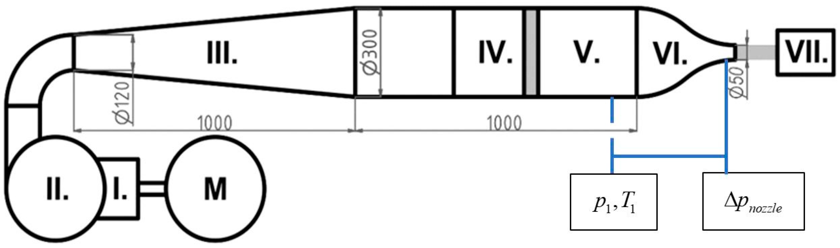
A special high-speed wind tunnel was used to verify the expected thermodynamic parameters of the designed probes. The high-speed track scheme is shown in Figure 1. The track consists of a total of five main parts: radial turbocharger, diffuser, air bleed system, plenum chamber, and high-contraction nozzle.
The electric motor is asynchronous, controlled by a frequency converter, with a rated power of 110 kW. Siemens Sinamics Micromaster STARTER software is used for remote control, allowing synchronous speed control from 100 to 3000 rpm. The compressor (HV Turbo A/S, Denmark, manufactured in 2002) is equipped with a 9:1 gearbox at the input. The compressor speed can therefore be controlled between 900 rpm and 27,000 rpm. The manufacturer specifies the maximum compression ratio of the compressor as 1.69 at maximum speed. The operating characteristics of the compressor have not been investigated, but its parameters allow achieving a nozzle outlet speed of about 280 m/s. The correlation between the compressor characteristics and the track characteristics causes a pumping mode of the compressor in the range of about 70 to 80% of the rated power, which must be eliminated by means of the air bleed system located between the diffuser and the plenum chamber. The outlet nozzle has a contraction coefficient of 36.
During operation, the static pressure and total temperature inside the plenum chamber and the pressure gradient at the nozzle were measured. The total temperature was measured using a Pt100 RTD sensor with a shaft length of 150 mm and a diameter of 3 mm. Due to the large contraction of the nozzle, the velocity in the plenum chamber was low enough to consider the measured airflow temperature static. The individual devices used to measure each quantity are listed in Table 1.
The Compact DAQ system from National Instruments was used for data acquisition. Specifically, it was a four-slot cDAQ 7194 chassis with individual dedicated modules for current measurement and temperature measurement using the RTD sensors NI-9203 and NI-9216, respectively. MATLAB software with appropriate drivers was used to control the measurement hardware and subsequent data evaluation.
The static temperature of the air that exited the nozzle was determined indirectly for calibration of the DRTA temperature probes. Its value calculation assumed that the flow of air through the nozzle is an isentropic expansion as follows:
where temperature and pressure represent the static values of pressure and temperature upstream the nozzle, and is the pressure drop in the nozzle. For the possibility of successful use of the high-speed track for verifying the parameters of the designed probes and their subsequent calibration, it was necessary to map the parameters of the flow field in the test section, which means in the area downstream the nozzle, where the probes were inserted for measurement. The two main parameters that needed to be experimentally measured were the velocity profile and the intensity of the turbulence.
(a) Velocity profile: The data rendered by the verified DRTA probe were compared with the velocity obtained from the Prandtl probe during calibration. The distance between the two probes was always kept as small as possible, but it had to be large enough so that the two probes did not interfere with each other. At the same time, it must be assumed that both probes operate under the same conditions, that is, that they are charged with the same velocity. The axial distance of the two probes (the Prandtl probe and the closer temperature probe) was chosen as the value ( = mean outer diameter). Therefore, the conclusion of these considerations was the requirement for a flat velocity profile in a sufficient neighborhood of the inserted probes.
(b) Turbulence intensity: This is not only a general quantity for evaluating the quality of the air flow entering the measuring space but also a parameter that has a significant influence on the value of the recovery factor of temperature probes. This issue has been addressed, for example, by Kulkarni, Madanan, and Goldstein, who in their paper [6] compared the recovery factor of a temperature probe for turbulence intensities of and In their conclusions, they described a significant effect on the recovery factor of the probe, with the observation that, for increasing values of the intensity of the turbulence of the incoming air stream, the recovery factor decreases significantly. Specifically, for their probe, the recovery factor was equal to the value for of the turbulence intensity and equal to the value of for of the turbulence intensity. At the same time, they concluded that their measured values are consistent with the deviation from the predictions of the probe recovery factor behavior as a function of the turbulence intensity made by Stinson and Goldstein [7]. Here, they considered the dependence of the thermocouple probe recovery factor on the value of the turbulence intensity. The probe was in the shape of a cylinder, placed perpendicular to the direction of the incoming air flow. They performed their experiments for Mach numbers ranging from 0 to 2 and for turbulence intensities ranging from to . The following equation was presented as the resulting relationship to predict the dependence of the recovery factor on the turbulence intensity of the incoming air stream.
The value of the turbulence intensity was evaluated according to the following equation:
where is the squared time mean value of the velocity fluctuations at a given point, and is the time mean value of the velocity at the same point [8]. The data were acquired at a sampling rate of 20 kHz, and the length of each recording was 20 s. A separate chapter of this article is devoted to the determination of the measurement uncertainties for each parameter.
The uncertainty analyses: Experimental results were evaluated and are presented in the form , where represents the evaluated quantity, shows its magnitude (measured directly or calculated), and is the expanded uncertainty, obtained by multiplying the combined standard uncertainty by a coverage factor . Typically, is in the range from 2 to 3, where, considering a normal distribution, the value of defines an interval having a level of confidence of approximately 95% and defines an interval having a level of confidence greater than 99%. The value of was used for the results presented in this article. The combined uncertainty was evaluated as a combination of uncertainties of Type A and Type B as follows:
The Type A uncertainty evaluation method is based on the statistical analysis of a series of observations (mean value and its standard deviation). On the other hand, Type B uncertainty evaluation is based on statistical analyses of recorded data (accuracy and precision of sensors, quality of the calibration, etc.).
During the evaluation of the experimental data presented in this article, data sets that contained hundreds of samples were always dealt with. Therefore, Type A uncertainty was neglected when evaluating the combined uncertainty, and the expanded uncertainty was calculated as follows:
Type B uncertainty, based on the accuracy of the sensors and transducers used, the geometric precision of the pressure probes, etc., was evaluated as
where represents the measured quantity (pressures, temperatures), corresponds to the uncertainty of its measurement, and is the sensitivity coefficient describing the propagation of the uncertainty of the measured quantity to the final value of . For indirect measurements, where the final quantity , the sensitivity coefficients are calculated as partial derivatives of function with respect to all measured quantities:
The uncertainty of mean velocity measurement.
The velocity of an undisturbed stream was measured indirectly with the help of a pitot-static tube. This means the final value of was calculated by the following equation:
where quantities were measured directly. The pressure difference in Equation (15) is the pressure difference in the pitot-static tube used for the velocity measurement, and represents the compressibility correction coefficient usually calculated as a function of the Mach number. According to Equation (13), the uncertainty was calculated as follows:
The sensitivity coefficients were calculated as follows:
where constant . The uncertainties for all measured quantities, based on manufacturer data or the calibration method, are shown in Table 2.
The same approach was also used to assess the uncertainties in measuring the intensity of the turbulence and assessing the recovery factor.
3. Results
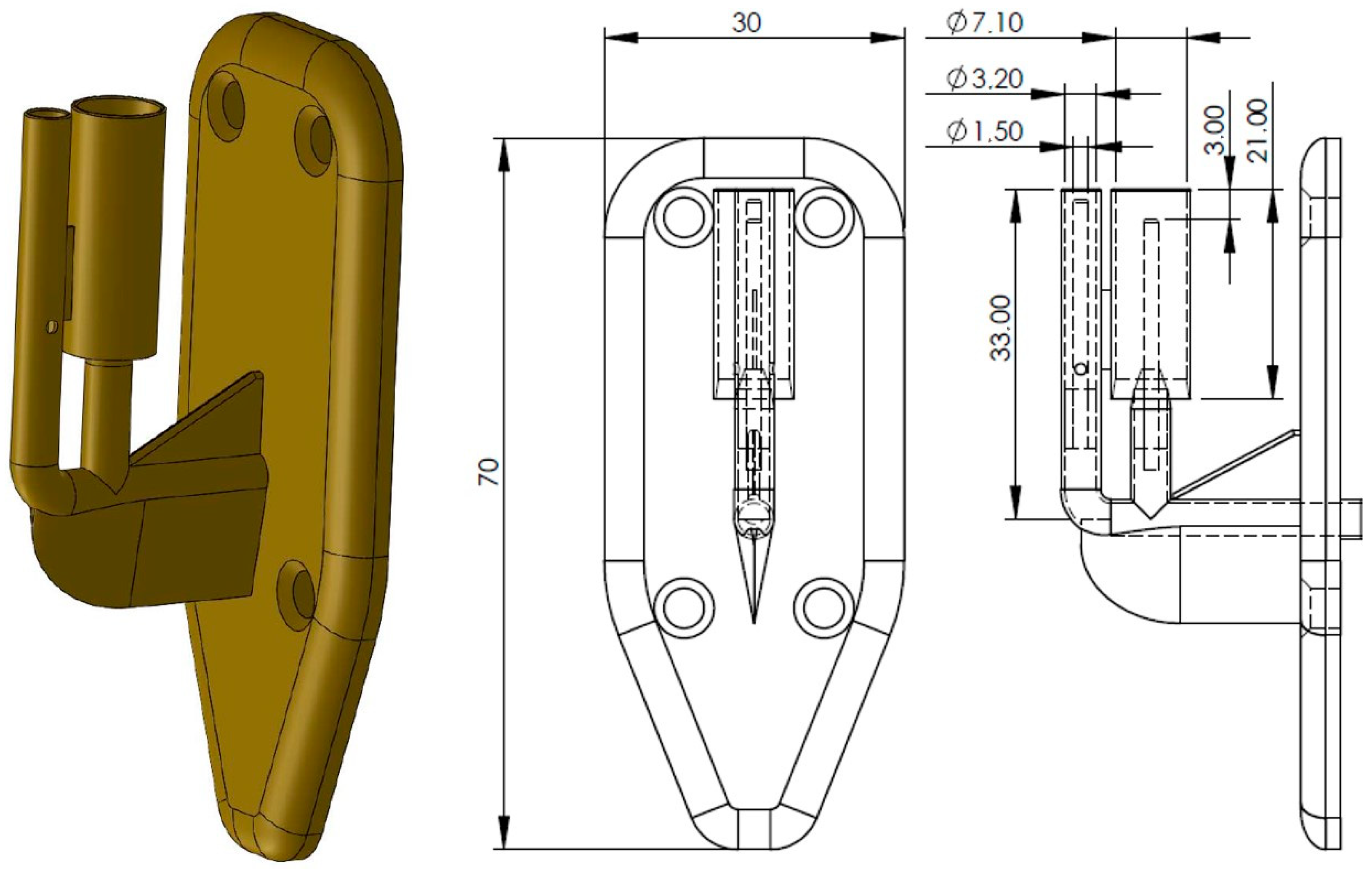
The final geometry of the designed multi-element temperature probe and its important parameters are described in this section. The results of the probe testing indicate its suitability for use as a probe for airspeed measurements. The described probe has undergone a long evolution and is currently the fourth modification of the original design. The DRTA probe, originally developed in 2020 to enable the measurement of compressible fluid flow velocity through the temperature measurements described in [4], has been modified in 2022 for use in high-radiant-energy flow environments. The latest proposed probe geometry is shown in the following figure. The temperature measurement is performed using two Pt100 sensors, which provide sufficient measurement accuracy. The sensors in this case are 25 mm long and have a diameter of 1.5 mm.
The last modification, shown in Figure 2, consisted in modifying the probe to allow its use in aviation. The probe is designed to be mounted on the outer skin of the aircraft, either on the fuselage or the wing.
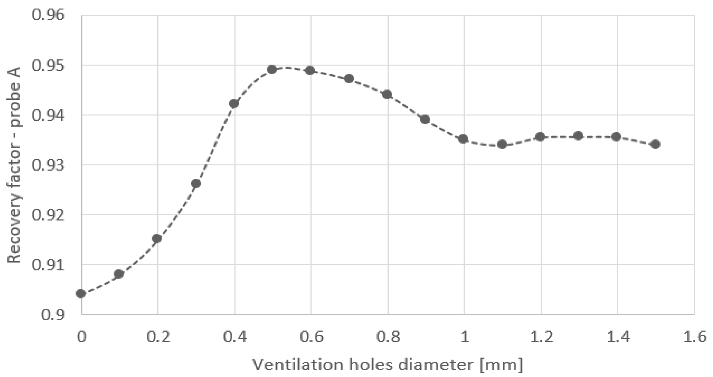
As shown by Villafae and Paniagua [9], the recovery factor value for a shielded probe was expected to be higher than the value for an unshielded probe. In this case, the shielded probe means probe A. Probe B, originally unshielded, was equipped with a shield that minimally affects the flow field in its vicinity, and its task is only to eliminate ambient thermal radiation. For the shielded temperature sensor, emphasis was placed on the ratio of the size of the input cross-section to the cross-section of the ventilation openings. As with the original probe, this was based on a study by Rom and Kronzon [10], where for a given probe geometry, the maximum recovery factor was achieved for a design with two ventilation holes with a diameter of 0.5 mm. The size of the ventilation holes was investigated by numerical simulations to determine the dependence of the recovery factor on the size of the ventilation holes. For the resulting geometry, the results of the numerical analyses were verified experimentally. All CFD analyses were performed using ANSYS Fluent software, and the results of the analyses are shown in Figure 3.
Numerical simulations were performed for a dry air model with a velocity of 250 m/s and a temperature of 300 K. A k-epsilon turbulence model that includes fluid heating due to boundary layer energy dissipation was used for the simulation. The turbulence intensity was chosen to be 2.5%, and the mixing length was 0.01 m. Much attention has been focused on testing the quality of the mesh as a very important parameter for the correct determination of the recovery factor. For the purpose of these simulations, 10 grid cells were placed across the boundary layer.
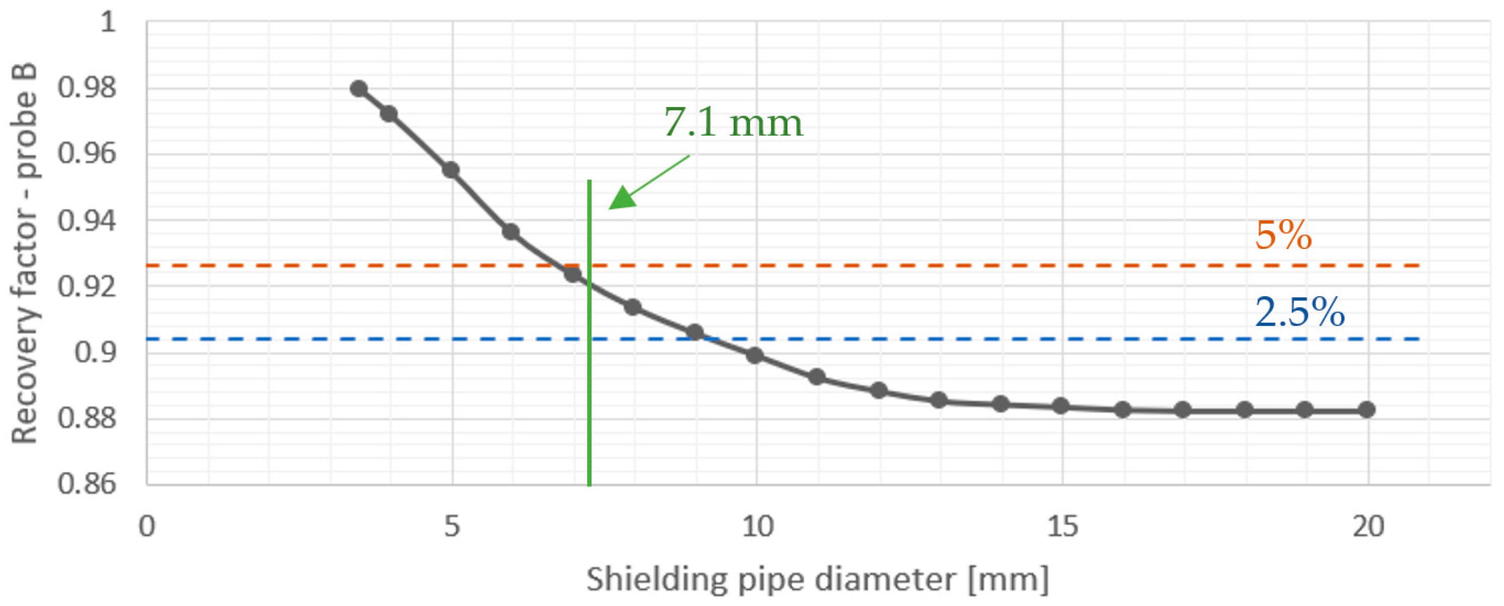
For probe B, however, it was necessary to achieve the lowest possible recovery factor. Again, numerical simulations were used for the correct probe design. In this case, the dependence of the recovery factor on the diameter of the probe shield was evaluated. The results are shown in Figure 4.
The diameter of the shielding tube chosen for the probe tested was 7.1 mm. As can be seen from the simulation results, the influence of probe B by the shield is less than 5%. It should be noted that in probe design, the choice of shielding tube diameter is always a compromise between the influence on the recovery factor and the directional insensitivity of the probe or other design conditions.
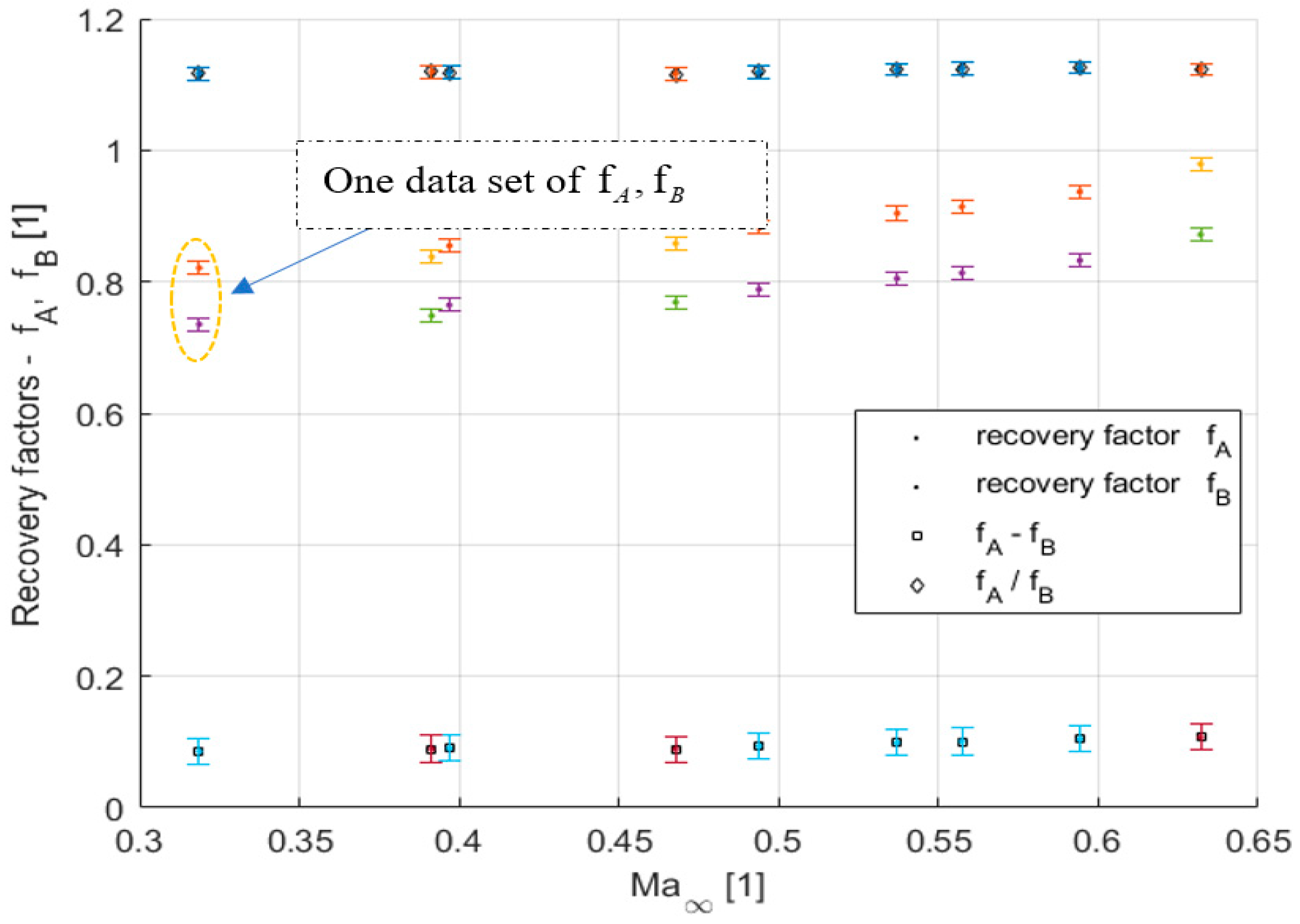
As mentioned previously, a sufficiently large difference between the two recovery factors is important for the successful use of a multi-element temperature probe for speed measurement and its sufficient sensitivity. The results of both recovery factors are shown in Figure 5.
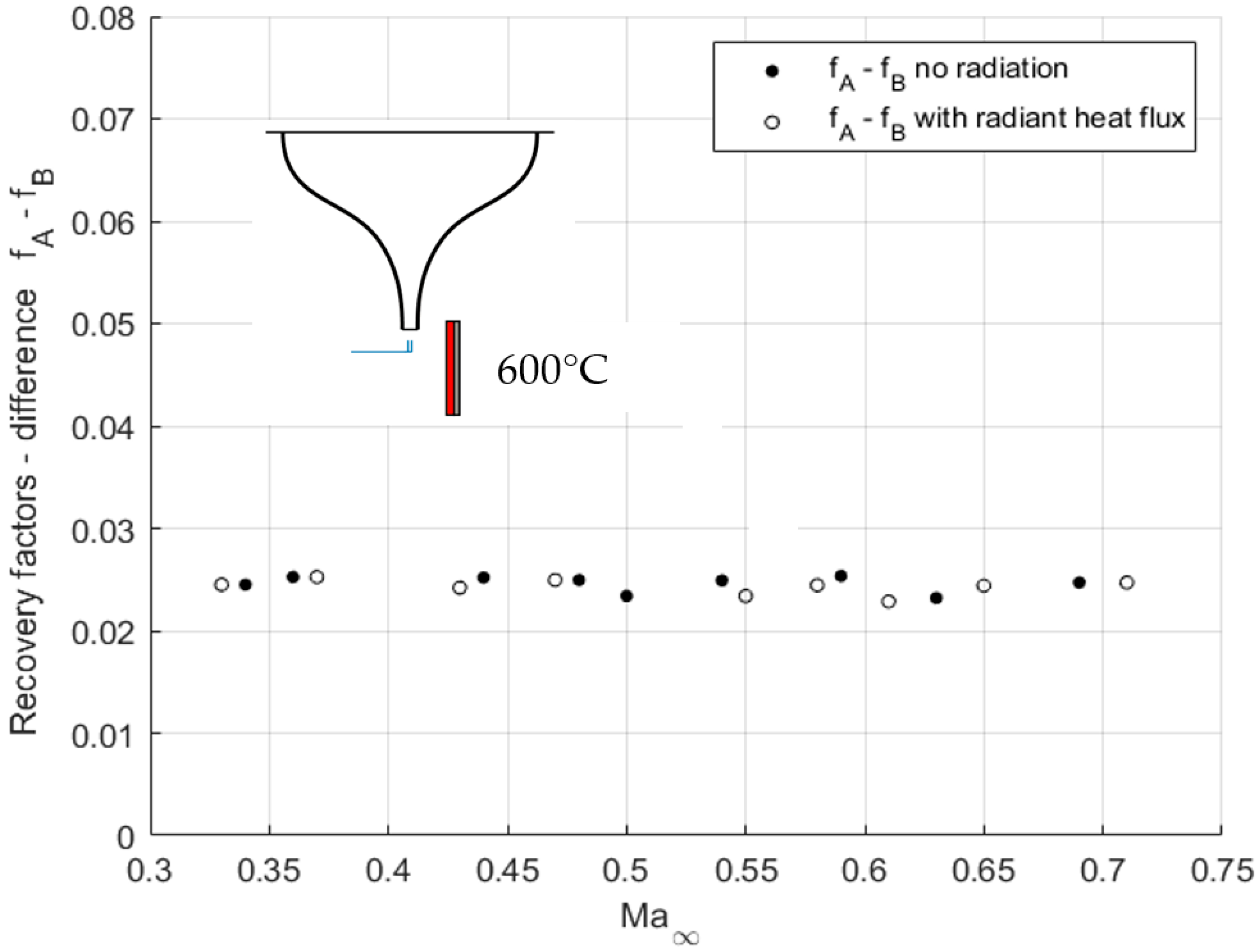
The measurements carried out showed not only a sufficiently large difference between the two recovery factors but also its sufficient independence from the Mach number. The stability of the difference in the recovery factors () is another important condition for the successful usability of the probe. The difference in the recovery factors of the two temperature sensors is shown as a dependence on the Mach number in the following Figure 6.
Due to the very small differences in the temperature measurements of the two temperature sensors, the heat flux into the probe body and the heat flux due to radiation from surrounding bodies play an important role. Therefore, the effect of the presence of a thermal emitter near the DRTA probe was also tested. The radiator was in the form of a flat plate with dimensions of 200 × 100 mm, and its surface was painted with a special paint with emissivity of 0.95. The radiator was heated to a temperature of 600 °C using resistive electrical elements. The radiator was placed 100 mm from the temperature probe, as shown in Figure 6.
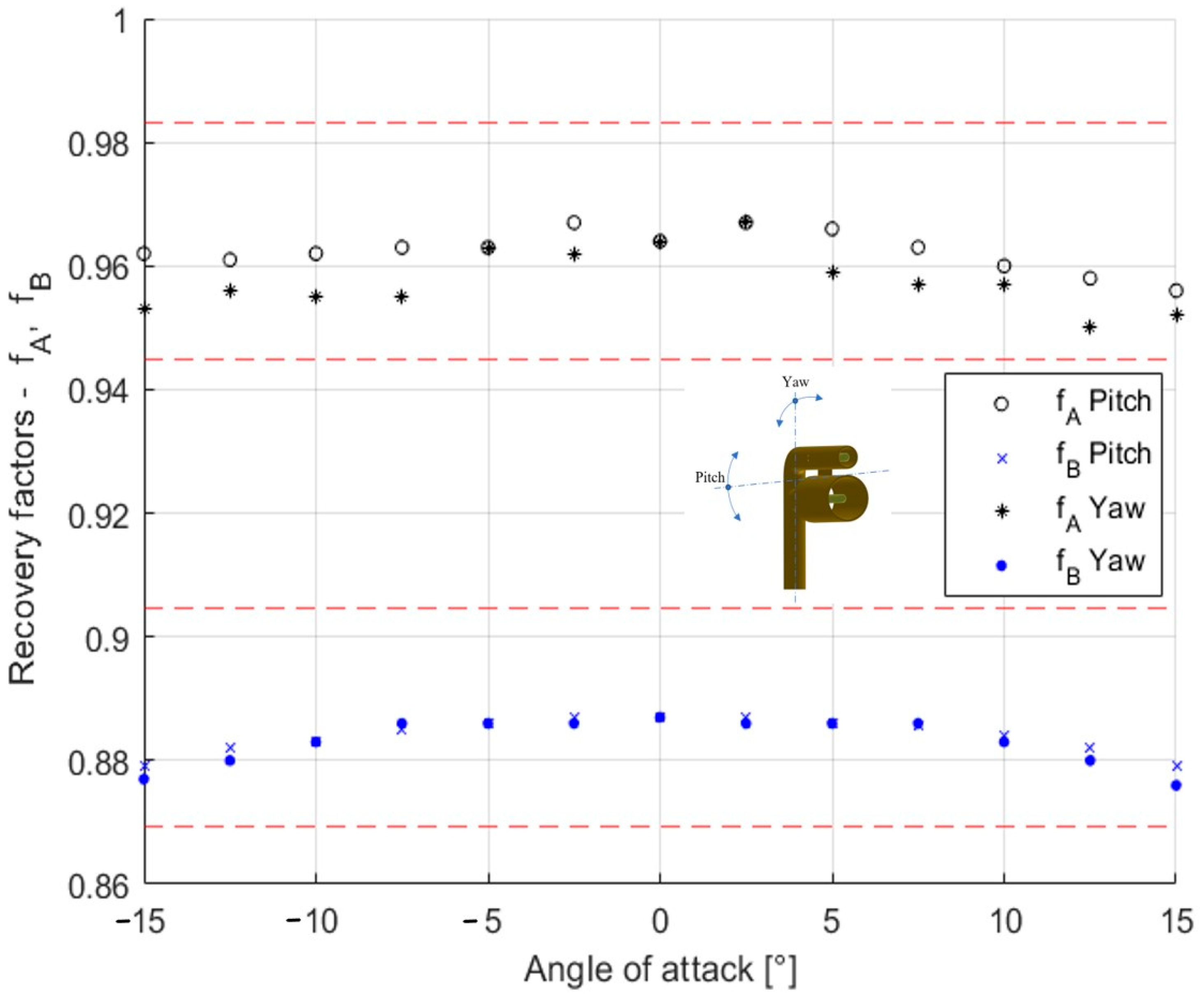
In the last step, the directional sensitivity of the developed DRTA temperature probe was tested. The dependence of the recovery factors of both sensors on the angle of attack of the probe was tested in both the pitch and yaw directions. The measurement results are shown in Figure 7.
The measurement results confirm the original assumptions about the high directional insensitivity of both temperature probes. Therefore, the proposed temperature probe can be used in the range of ±15° with an error of less than 2%.
4. Discussion
A multi-element temperature probe designed to be used for the measurement of the speed of flight of subsonic aircrafts was described in this article. Although the probe can also be used for supersonic speed, this issue was not discussed here in the article because it represents a challenge in its own right. In any case, there is always a problem of compressible fluid flow. Generally speaking, the principle of the described probe is based on the method called RTA (Recovery Temperature Anemometry). A modification of this method using multiple temperature sensors with different recovery factors results in the DRTA method (Double-sensor Recovery Temperature Anemometry).
It is known that the recovery factor of the temperature probe depends on many parameters such as the Reynolds number, Mach number, physical properties of the flowing fluid, and turbulence intensity. The main advantage of the application of two probes with different recovery factors is that there is only the need for knowing the difference between both recovery factors of the used probes, as described in Equation (7). Due to the location of the probes close to each other, it can be assumed that the change in the recovery factors of both probes will be the same and the difference in their values will remain constant. This was confirmed by the experiments performed, in which the flow velocity of the inflowing air and its temperature were different, as shown in Figure 5 or Figure 6.
The experiments performed showed the constant difference in the recovery factors even if both were not constant individually. This confirmed the main premise for the helpful use of this probe for the airflow velocity measurement. The situation is more complicated in the case of the Mach number evaluation. The Mach number can be evaluated as follows:
Unfortunately, in this case, the dependence is not only on the difference between the two recovery factors but also on its absolute value. It is obvious that a greater difference in the recovery factors for the two probes used means a better sensitivity and accuracy of the probe. That is why our previous research work was focused on finding the best geometry of subsonic DRTA probes that show the best possible sensitivity and accuracy.
Many sources describe the best design of probes to measure the stagnation temperature, whose recovery factors are relatively high, up to a value of 0.98. The goal for future research work is to build such a temperature sensor into the DRTA probe, which will significantly increase its sensitivity. For now, the CFD simulation was used for the determination of the best size of ventilation holes for the total temperature probe, where the best ratio between the size of the inlet area cross-section and the area of the ventilation holes was determined as 16 with the probe A recovery factor of 0.968.
5. Conclusions
This article presents the results of many years of research in the field of high-speed temperature probes and the possibility of their use in aircraft airspeed measurements. Although this article essentially focuses on the presentation of the most important features of these probes, the author aims to open the space for their deployment in aviation, which is also reflected in the title of the article.
This article briefly describes the principle of operation of these high-speed probes, the conditions used for their testing, and the analysis of measurement uncertainties. Furthermore, the following properties of the proposed probe are presented in this article:
- -
- A geometric design with the main dimensions—the main dimensions of the probe are shown in Figure 2.
- -
- Detailed analysis of the effect of the size of the vents on the recovery factor of probe A: based on the results of the numerical analysis, two ventilation holes with a diameter of 0.5 mm were used for the given geometry. In general, it seems best to keep the ratio of probe inlet area to vent area equal to 16.
- -
- A detailed analysis of the effect of the diameter of the shielding tube on the recovery factor of probe B: in general, the larger the diameter of the shielding tube, the smaller the effect on the recovery factor. However, the design is always a compromise with respect to other design options. When using a 7.1 mm-diameter shielding tube (for a 1.5 mm-diameter sensor), the increase in the recovery factor is up to 5%.
- -
- The dependence of the recovery factors of probe A and probe B on the Mach number; the experimental results showed the independence of the difference between the recovery factors of probe A and probe B on the Mach number as a great advantage when using this probe for velocity measurements.
- -
- The independence of the probe from ambient thermal radiation was confirmed experimentally.
- -
- The directional sensitivity of the probe; the experimental results confirmed the high directional insensitivity of the probe, which can be used at angles of attack of ± 15° with an error of up to 2%.
The author believes that the information presented will be useful to other scientists working on the development of high-speed probes.
Funding
This research was funded by Czech Technical University in Prague, grant number RVO12000.
Data Availability Statement
Not applicable.
Acknowledgments
The author would like to express his deep gratitude to the Czech Technical University in Prague, Faculty of Mechanical Engineering, for providing the laboratory facilities and equipment necessary to perform the presented experiments.
Conflicts of Interest
The author declares no conflict of interest. The funders had no role in the design of the study; in the collection, analyses, or interpretation of data; in the writing of the manuscript; or in the decision to publish the results.
Nomenclature
| Latin: | Unit: | Description: |
| sensitivity coefficient: uncertainty calculation | ||
| [ms−1] | free-stream velocity | |
| [ms−1] | velocity fluctuation | |
| [J·kg−1K−1] | specific heat at constant pressure | |
| recovery factor | ||
| turbulence intensity | ||
| coverage factor, expanded uncertainty calculation | ||
| the compressible flow correction coefficient | ||
| static pressures upstream/downstream of the nozzle | ||
| pressure difference through the nozzle | ||
| stagnation and static pressure difference in a pitot-static tube | ||
| [J·kg−1K−1] | specific gas constant | |
| thermodynamic temperature | ||
| temperature of the fluid upstream of the nozzle | ||
| recovery temperature | ||
| free-stream temperature | ||
| uncertainty, Type B | ||
| expanded uncertainty | ||
| Greek: | ||
| heat capacity ratio | ||
| [kg·m−3] | the density of air | |
| Dimensionless: | ||
| Mach number | ||
| Prandtl number | ||
| Subscripts: | ||
| A, B | - | quantities related to both temperature sensors A and B |
References
- Anderson, J.D. Modern Compressible Flow, 2nd ed.; McGraw-Hill: New York, NY, USA, 1990; ISBN 0-07-001673-9. [Google Scholar]
- Ishibashi, M. pRTA (Probe Recovery Temperature Anemometry). In Proceedings of the ASME 2004 Heat Transfer/Fluid Engineering Summer Conference, Charlotte, NC, USA, 11–15 July 2004; pp. 613–618. [Google Scholar]
- Ishibashi, M.; Morioka, T. Velocity field measurements in critical nozzles using Recovery Temperature Anemometry (RTA). Flow Meas. Instrum. 2012, 25, 15–25. [Google Scholar] [CrossRef]
- Schmirler, M.; Krubner, J. Double probe recovery temperature Anemometry. Therm. Sci. Eng. Prog. 2021, 23, 100875. [Google Scholar] [CrossRef]
- Shapiro, A.H. The Dynamics and Thermodynamics of Compressible Fluid Flow; The Ronald Press Company: New York, NY, USA, 1953; Volume 1. [Google Scholar]
- Kulkarni, K.S.; Madanan, U.; Goldstein, R.J. Effect of freestream turbulence on recovery factor of a thermocouple probe and its consequences. Int. J. Heat Mass Transfer. 2020, 152, 119498. [Google Scholar] [CrossRef]
- Stinson, M.; Goldstein, R.J. Effect of freestream turbulence on recovery factor of a cylindrical temperature probe. In Proceedings of the First Thermal and Fluids Engineering Summer Conference, New York, NY, USA, 9–12 August 2015; pp. 945–958. [Google Scholar] [CrossRef]
- Bruun, H.H. Hot-Wire Anemometry. Principles and Signal Analysis, 1st ed.; Oxford Science Publications: Oxford, UK, 2009. [Google Scholar] [CrossRef] [Green Version]
- Villafane, L. Aero-thermal analysis of shielded fine wire thermocouple probes. Int. J. Therm. Sci. 2013, 65, 214–223. [Google Scholar] [CrossRef]
- Rom, J.; Kronzon, Y. Small-Shielded Thermocouple Total Temperature Probes; AD668466, TAE Report No.79; Israel Institute of Technology: Haifa, Israel, 1967. [Google Scholar]
Figure 1.
Scheme of the used high-speed track: M, electric motor; I., silencer in the compressor suction; II., radial turbocompressor; III., diffuser; IV., bleed valve; V., plenum chamber with static pressure and total temperature measurement; VI., nozzle; VII., test section.
Figure 1.
Scheme of the used high-speed track: M, electric motor; I., silencer in the compressor suction; II., radial turbocompressor; III., diffuser; IV., bleed valve; V., plenum chamber with static pressure and total temperature measurement; VI., nozzle; VII., test section.

Figure 2.
The final geometry of the proposed multi-element temperature probe for speed of flight measurement. (Left): 3D model, (right): main dimensions.
Figure 2.
The final geometry of the proposed multi-element temperature probe for speed of flight measurement. (Left): 3D model, (right): main dimensions.

Figure 3.
The dependence of the recovery factor of probe A on the size of the ventilation openings; CFD simulation results.
Figure 3.
The dependence of the recovery factor of probe A on the size of the ventilation openings; CFD simulation results.

Figure 4.
The dependence of the recovery factor on the probe B shield diameter; CFD simulation results.
Figure 4.
The dependence of the recovery factor on the probe B shield diameter; CFD simulation results.

Figure 5.
Results of the experimental investigation of the recovery factors of both temperature sensors of a multi-element temperature probe designed for airspeed measurement.
Figure 5.
Results of the experimental investigation of the recovery factors of both temperature sensors of a multi-element temperature probe designed for airspeed measurement.

Figure 6.
Measured difference in recovery factors as a function of the Mach number. The effect of the presence of a 600 °C radiator on the measured data was also tested.
Figure 6.
Measured difference in recovery factors as a function of the Mach number. The effect of the presence of a 600 °C radiator on the measured data was also tested.

Figure 7.
The recovery factors of both temperature sensors as a function of the angle of attack. The 2% insensivity bands are shown by the red dashed lines.
Figure 7.
The recovery factors of both temperature sensors as a function of the angle of attack. The 2% insensivity bands are shown by the red dashed lines.


Table 1.
Quantities measured on the aerodynamic track and related equipment.
| Quantity | Device | Description |
|---|---|---|
| Absolute pressure transducer | BD Sensors, type XMPi, range 0–2 bar abs., uncertainty 0.1% FS, output sig. 4–20 mA. | |
| RTD sensor Pt 100 | Pt 100, three wire, diam. 3 mm, temp. range −50 °C up to +250 °C, manuf. Omega Engineering, series PR–10. | |
| Differential pressure transducer | BD Sensors, type XMD, range 0–2 bar diff., uncertainty 0.1% FS, output sig. 4–20 mA. |
Table 2.
Uncertainties of Type B for all measured quantities for velocity evaluation.
| Name | Value | Description |
|---|---|---|
| K | Pt100, platinum temperature sensor | |
| Pa | A differential pressure transducer, range 40 kPa, 0.1% FS | |
| Pa | A differential pressure transducer, range 2 bar, 0.1% FS | |
| Pa | An absolute pressure transducer, range 2 bar, 0.1% FS | |
| K | Pt100, platinum temperature sensor |
Publisher’s Note: MDPI stays neutral with regard to jurisdictional claims in published maps and institutional affiliations. |
© 2022 by the author. Licensee MDPI, Basel, Switzerland. This article is an open access article distributed under the terms and conditions of the Creative Commons Attribution (CC BY) license (https://creativecommons.org/licenses/by/4.0/).
Share and Cite
MDPI and ACS Style
Schmirler, M. Flight Speed Evaluation Using a Special Multi-Element High-Speed Temperature Probe. Aerospace 2022, 9, 185. https://doi.org/10.3390/aerospace9040185
AMA Style
Schmirler M. Flight Speed Evaluation Using a Special Multi-Element High-Speed Temperature Probe. Aerospace. 2022; 9(4):185. https://doi.org/10.3390/aerospace9040185
Chicago/Turabian StyleSchmirler, Michal. 2022. "Flight Speed Evaluation Using a Special Multi-Element High-Speed Temperature Probe" Aerospace 9, no. 4: 185. https://doi.org/10.3390/aerospace9040185
Note that from the first issue of 2016, this journal uses article numbers instead of page numbers. See further details here.