Application of Probabilistic Set-Based Design Exploration on the Energy Management of a Hybrid-Electric Aircraft

Abstract

The energy management strategy of a hybrid-electric aircraft is coupled with the design of the propulsion system itself. A new design space exploration methodology based on Set-Based Design is introduced to analyse the effects of different strategies on the fuel consumption, ${\mathrm{NO}}_{\mathrm{x}}$ and take-off mass. Probabilities are used to evaluate and discard areas of the design space not capable of satisfying the constraints and requirements, saving computational time corresponding to an average of 75%. The study is carried on a 50-seater regional turboprop with a parallel hybrid-electric architecture. The strategies are modelled as piecewise linear functions of the degree of hybridisation and are applied to different mission phases to explore how the strategy complexity and the number of hybridised segments can influence the behaviour of the system. The results indicate that the complexity of the parametrisation does not affect the trade-off between fuel consumption and ${\mathrm{NO}}_{\mathrm{x}}$ emissions. On the contrary, a significant trade-off is identified on which phases are hybridised. That is, the least fuel consumption is obtained only by hybridising the longest mission phase, while less ${\mathrm{NO}}_{\mathrm{x}}$ emissions are generated if more phases are hybridised. Finally, the maximum take-off mass was investigated as a parameter, and the impact to the trade-off between the objectives was analysed. Three energy management strategies were suggested from these findings, which achieved a reduction to the fuel consumption of up to 10% and a reduction to ${\mathrm{NO}}_{\mathrm{x}}$ emissions of up to 15%.

1. Introduction

Electrification has been at the forefront of sustainable aviation research for the last 10 years. Projects such as the European Union’s FlightPath 2050 seek to reduce the ${\mathrm{CO}}_2$ and ${\mathrm{NO}}_{\mathrm{x}}$ emissions of the commercial fleet by 75% and 90%, respectively, compared to the best-of-class in 2000 [1]. These goals fall within a global trend of aviation de-carbonification measures proposed by the ICAO [2]. One type of electrified aircraft concept is the hybrid-electric aircraft (HEA), where the power required for propulsion is supplied by more than one type of energy source, usually fuel and batteries [3,4]. Hybrid propulsion is proposed as a stepping stone towards full electrification, as future electric technologies are expected to be inadequate for achieving enough range to be competitive with conventional commercial aircraft [5].

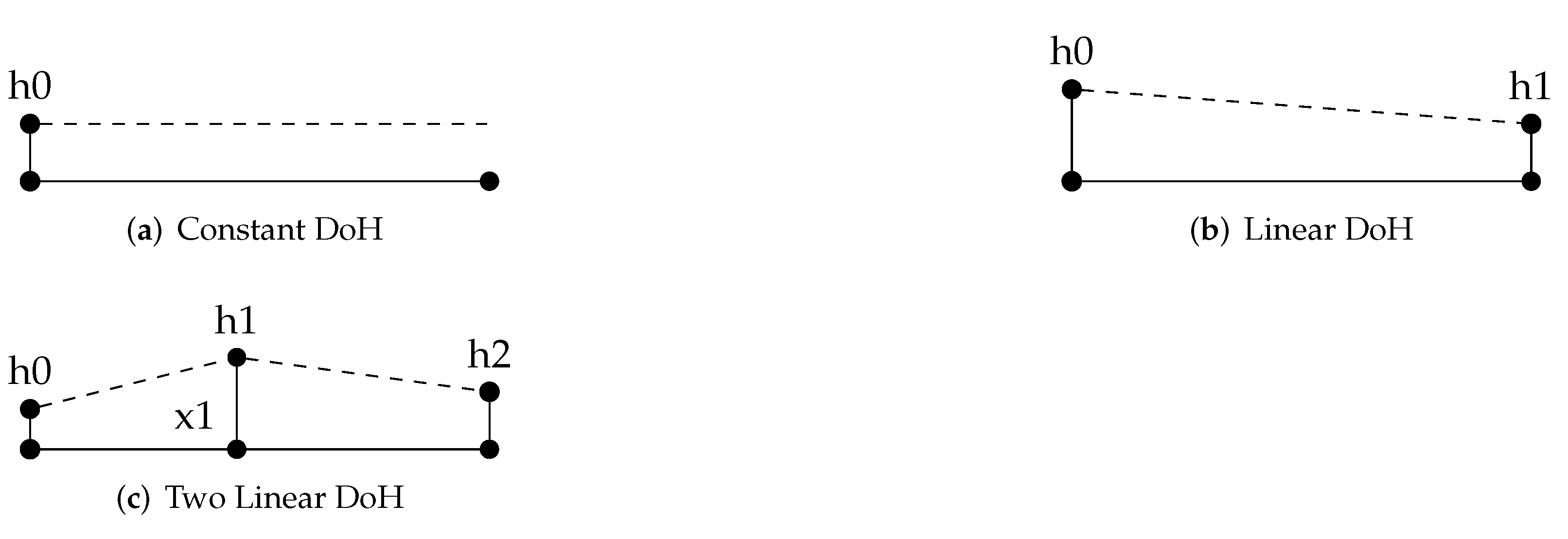
Unlike other propulsion systems, HEAs have multiple energy sources and power distribution paths. An Energy Management Strategy (EMS) can be introduced to find the optimal use of the available energy for a defined mission. EMS is a function of the degree of hybridisation (DoH) [6] of the power over time, where DoH is the ratio of the power that is supplied by the electric source over the overall power required by the aircraft at that point in time. This single parameter is sufficient if there are only two power paths. Otherwise, multiple non-dimensional parameters have to be specified for each path, such as how much energy is provided by batteries over the total electrical power production if the system has multiple electrical power sources [3,4].

The problem of specifying an optimal EMS is complicated by how unpredictable its operational conditions can be. The HEA can operate between any airports within its maximum range and service ceiling. The approaches to solve this problem are divided into two families: offline methods and online methods [7,8]. The offline approaches find the optimal strategy by simulating the vehicle’s operational life and tuning the parameters of the EMS. Some examples include heuristic rules [9], fuzzy control [10] and global optimisation algorithms such as dynamic programming [11]. On the contrary, online methods tune the EMS during the vehicle operation, such as Pontryagin’s Maximum Principle [12].

However, few studies have been published where the EMS and HEPS sizing are coupled [13,14,15,16]. Indeed, the EMS of an HEA has to address the change in power requirements from the change in aircraft mass during its operation, which is not present in HE land vehicles. In this respect, two opposite approaches are generally adopted. The first one consists of considering a fixed energy management strategy, usually a uniform degree of hybridisation over cruise and climb, and the size of the aircraft according to the energy requirements. This approach is usually selected to study and compare different HE architectures and can be found in Pornet [13] and Zamboni [14]. The other approach is to iteratively couple the energy management optimisation with the system sizing. Trawick [15] implemented a global optimisation methodology where dynamic programming is used to construct the optimal EMS and sequentially size the system. This approach is more flexible since it does not assume any analytical form of the power schedule but calculates the optimal schedule by starting from the end state of the aircraft and searching backwards the optimal power setting that minimises the objective function. The drawback is the high memory and computational cost, as the algorithm has to evaluate $N\times M^2$ states when searching for the optimal path, assuming a single-setting discretised M times over N time steps.

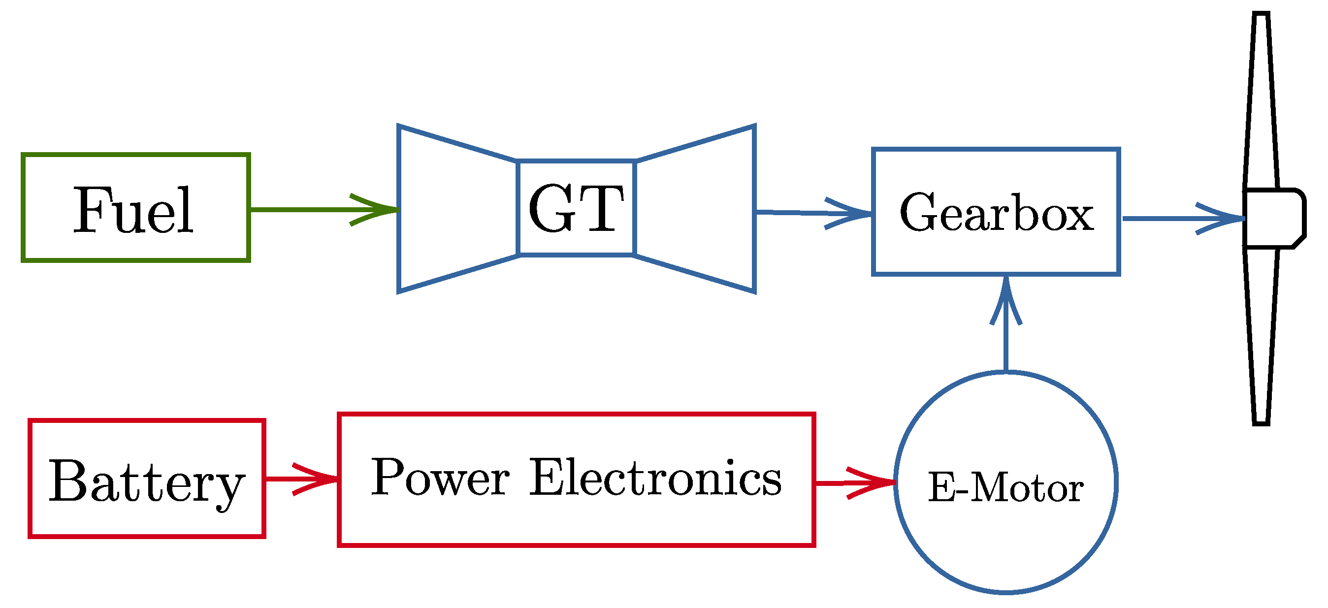
The presented work tries to implement a new design space exploration methodology to study the coupling between the EMS and the HEPS. For this reason we selected an architecture that is well-studied in the literature [17,18,19,20,21,22,23,24,25] and is the most mature within the FutPrint50 project. Regarding the modelling of the EMS, an intermediate approach is adopted where the class of possible DoH functions are restricted within the set of polynomial functions. Then, the design space methodology searches for the parameters that minimise fuel consumption and ${\mathrm{NO}}_{\mathrm{x}}$ emissions. At each iteration, the evaluation function sizes the mass of required fuel and batteries, taking into account the power–mass coupling. The goal is to identify an optimal energy management strategy for a given mission and value of maximum take-off mass.

The problem of finding the EMS that satisfies the requirements and constraints of the system under design is an engineering design problem. Hence, the design space exploration and optimisation techniques are required. A significant challenge in this field is handling the complex interactions and feedbacks between multiple subsystems [26].

Several approaches have been developed, which can be divided into two families: an iterative or point-based approach and a convergent or parallel-based approach. In the first type, a candidate design or solution is selected from an initial trade-off analysis and refined with several iterations with optimisation tools and higher fidelity analysis. This approach is the traditional process of conceptual, preliminary and detail design, often called the “waterfall model” in software engineering. Examples of this approach can be found in Ullman [27] and Pahl [28]. In the context of design space exploration, the Margin Value Method [29] is a point-based approach that, from a starting configuration, identifies excessive margins, any parameter that sub-optimally satisfies the constraints and evaluates the possible improvement by quantifying the trade-off between robustness and performance degradation. Guenov [30] presents a Margin Allocation method to dynamically assess the effect of margins on performance, other margins and constraint satisfaction, so that the designer can understand the interactions between the system under design, its components and the overall requirements.

Conversely, the second type considers and evolves many candidate designs in parallel, discarding the unfeasible, undesirable or non-robust ones. Design methodologies that fall within this category are the Method of Controlled Convergence of Pugh [31], the Design–Build–Test cycle of Wheelwright [32] and Set-Based Design (SBD) [33,34].

This paper focuses on Set-Based Design, whose principle is to generate as many configurations and delay critical design decisions as much as possible [35]. The aim is to avoid problems that often surface at advanced stages of the design process, which would require a major redesign or reversal of early decisions, prompting an increased cost both in terms of time and resources [36]. Set-Based Design has been recently investigated for the problem of designing products under flexible requirements [37,38], and incorporate resilience to unexpected modes of operation [39]. Furthermore, the large sweeping of the design space combined with a multi-disciplinary model makes SBD principles suitable for design space exploration and trade-off activities of complex systems [40]. SBD has also been applied in decision analysis, where it has been combined with Value of Information methods, enabling robust design selection [41,42].

The framework developed for this study combines set-based design with multi-objective optimisation. Most optimisation methods are point-based in nature, where single designs are optimised; hence, several authors have attempted to extend these for design sets.

Some authors use a multi-objective optimiser to search for the optimal set or family of solutions without exploring the individual designs. Sets are evaluated based on abstract quantities such as general optimality, variability, robustness [43], hypervolume size and imprecision [44]. Trade-off studies are performed. Some examples of this general approach are the Set-Based Concept method [43,45], the Set Swarm Optimisation [46] and the Set-Based Genetic Algorithm [44].

In contrast, others use SBD principles to reduce the searchable design space before introducing the optimiser. These approaches evaluate sets by mapping their input parameters to the optimisation objectives [47]. The final result expresses multiple individual designs that belong to the surviving sets.

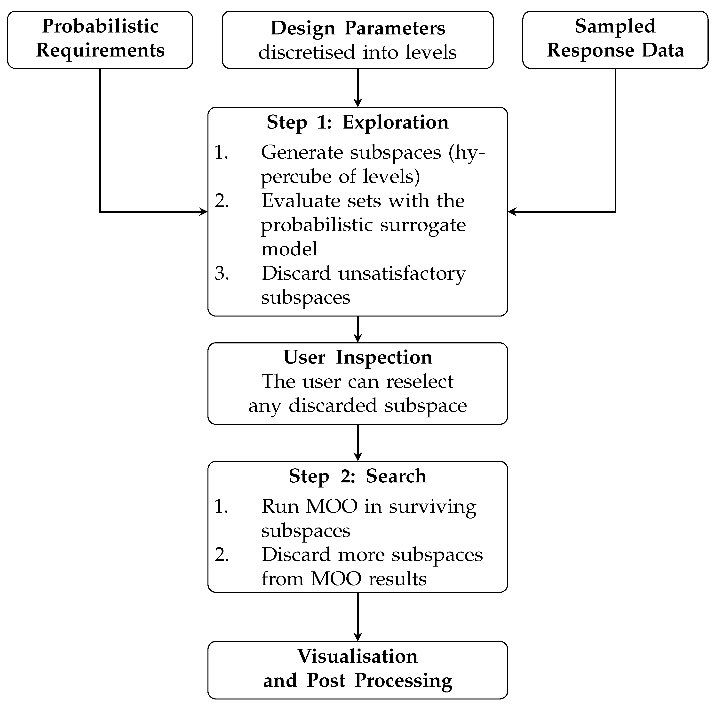
Some examples are the Set-Based MDO of Hannapel [48], the Technology Charaterization Models method [47] and the ADOPT framework [49]. The last one was chosen as it allows us to study the interaction between the input parameters and the design requirements. Furthermore, it allows us to identify and reject areas of the design space which are unable to satisfy the top-level requirements. However, the major drawback of this framework is the necessity of expertise on the problem under design for constructing if–else expert rules capable of filtering out unfeasible and undesirable configurations. Otherwise, even with a moderate number of parameters, the combinatorial explosion makes the entire methodology impractical to use. In fact, one major challenge in SBD methodologies is identifying the sets or subspaces out of all the possible combinations of discretised inputs that satisfy the requirements and discarding those that do not. Previous approaches can be divided into three main categories:

• Algorithmic approaches which classify the sets by propagating constraints. Examples include Constraint Satisfaction solvers [50,51] and Fuzzy Set theory [52].
• Machine Learning classification which constructs a decision boundary based on samples responses. Examples include Bayesian network classifiers [53], Support Vector Machines [47] and k-Means Clustering [54].
• Decision-based approaches which model the restriction of the design space as a transition between states. Examples include Markov Decision Processes [55] and Reinforcement Learning [56].

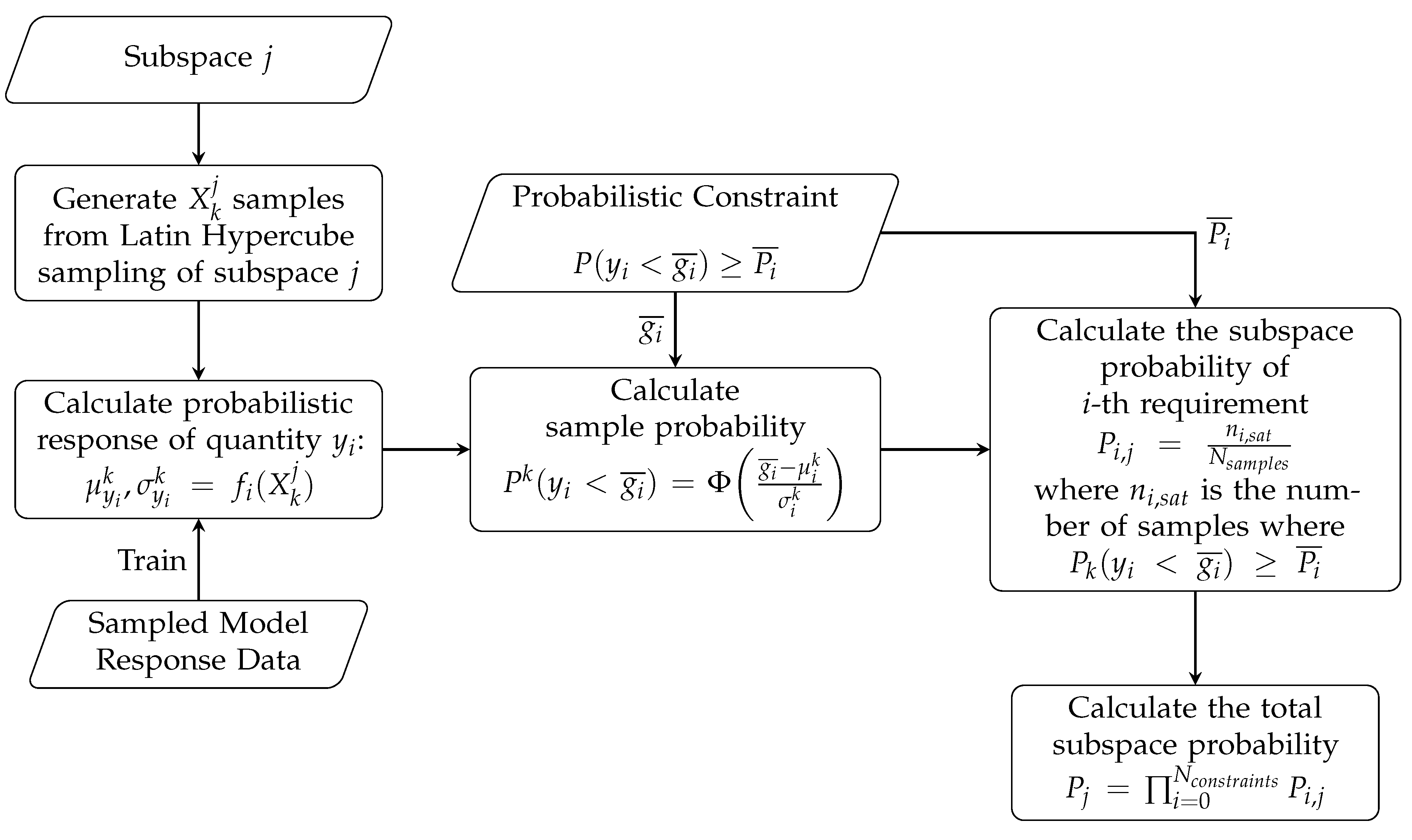
These approaches offer a deterministic classification of desirability of each design space subset. In the methodology presented in this paper the quantification of the uncertainty of the mapping procedure is considered. A Gaussian Process Regression was adopted to evaluate the capability of each set to satisfy the requirements and constraints. While this mathematical tool falls within the family of Machine Learning approaches, it provides an estimation of the variance of its response [57], hence enabling a probabilistic assessment of the design space [58].

While the application of probability theory has been widely used for the propagation of uncertainties on system performance [59,60], robust optimisation [61] and sensitivity analysis [62], it has been rarely used to assess the uncertainty of top level design requirements satisfaction. The previous use of probabilities in the context of top-level requirements satisfaction has been found recently in Guenov [30] and Di Bianchi [63]. Both authors use probabilities to estimate the ability of a design to satisfy the constraints, given some uncertainty: specifically on the margin for Guenov and on the constraint values for Di Bianchi. We seek to explore this approach and apply it in the context of Set-Based Design Optimisation.

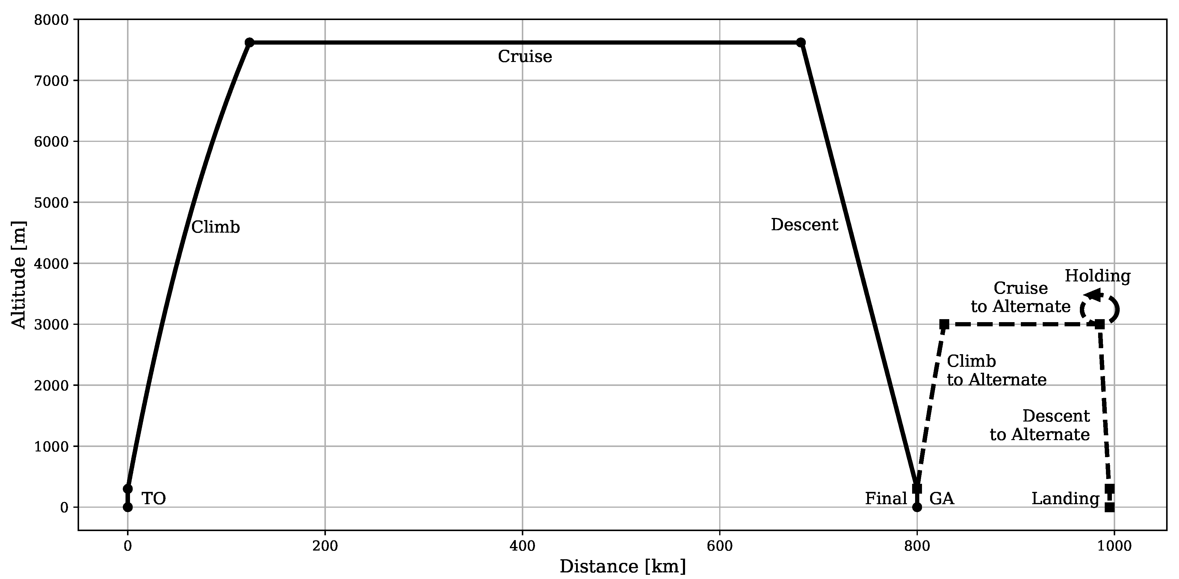
In this paper, Section 2 describes the modeling and methodologies adopted for this study with Section 2.1, focusing on the new design exploration framework, while Section 2.2 and Section 2.3 describe the parametrisation of the energy management schedule and the overall sizing and analysis of the hybrid-electric propulsion system. Section 3 presents the baseline aircraft, the sizing mission, the selected hybrid-electric propulsion architecture and the matrix of experiments performed in this study. Section 4 presents the results of these experiments, both from the perspective of the methodology (Section 4.1) and the energy management scheduling problem (Section 4.2, Section 4.3 and Section 4.4). These are discussed in Section 5.1, Section 5.2, Section 5.3, and Section 5.4, respectively. Finally, three families of energy management strategies were recommended in Section 5.5, and the findings are summarised in Section 6.

2. Materials and Methods

2.1. Design Exploration Methodology

The present methodology implements and extends the previous work by Georgiades [49], which employs a two-step process to explore and refine the design space with a convergent approach. Here, the principles of Set-Based Design are implemented with the enumeration of all possible combinations of discrete input parameter levels. These design “subspaces” are evaluated and discarded according to a set of feasibility and desirability rules, which encode the expert knowledge of the system under design. Then, an optimisation algorithm is used to search the surviving subspaces for the best design points. This new information is used by the designer to further discard areas of the design space and continue the convergence towards a final set of candidate solutions.

This method is improved by replacing the feasibility and desirability rules with a statistical response approach, which seeks to estimate the probability to satisfy the optimisation constraints and, if known, to bound the objectives. This second type of constraint is a “soft constraint” defined as a minimum desired outcome from the optimisation. For instance, if the designer desires the model to have no more than a value f for the objective to be minimised F, the framework allows us to introduce the constraint $F\left(x\right)<f$ to discard the areas of the design space that, even if minimised, will not meet this desired objective. This approach allows us to replace the desirability rules used previously [58]. Figure 1 presents the flowchart of the improved methodology.

The exploration step, where areas of the design space are marked as discarded and ignored, is necessary to avoid the combinatorial explosion of a traditional full search while allowing for alternatives that could be less performing but more robust. Equation (1) defines the number of total subspaces given $n_{par}$ parameters, where each k-th parameter has $l_k$ levels. For example, two parameters such as climb DOH and cruise DOH (both ranging between 0 and 1), divided into 4 levels each would generate 16 subspaces such as [(0–0.25), (0–0.25)] (level 0 of both parameters) or [(0.5–0.75), (0.25–0.5)] (level 1 and level 2).

Table 1. Total number of subspaces for different numbers of parameters and levels.

${\mathit{n}}_{\mathit{par}}$	$\mathit{l}=2$	$\mathit{l}=3$	$\mathit{l}=4$	$\mathit{l}=5$
2	4	9	16	25
3	8	27	64	125
4	16	81	256	625
5	32	273	1024	3125
6	64	729	4096	15,625

shows how rapidly the number of subspaces can grow even with a moderate number of discrete input parameters.

$$N_{subspace}=\prod _{k=0}^{n_{par}}{l}_k$$

(1)

The evaluation of each subspace is carried out with a statistical surrogate model trained for each of the constraints, returning its response and its standard deviation. Gaussian processes, reliably used in surrogate modeling [64], are employed which have the advantage of returning the statistical momentum of a Gaussian distribution as output for its trained inputs. This allows us to calculate the probability over a single sample using the Gaussian cumulative distribution function $\mathsf{\Phi }$, as described next. The implementation used is the Gaussian Process Regressor algorithm of scikit-learn Python library [65].

Let $y_i$ be a quantity of interest from the model under design $F\left(X\right)$, which is constrained by the inequality $y_i<\overline{g_i}$. Then, the target probabilities for this constraint $\overline{P_i}$ are defined such that:

$$P(y_i<\overline{g_i})\ge \overline{P_i}$$

(2)

Next, the probability to satisfy this constraint for a single sample in the design space, defined by the vector of parameters $X_k=\{x_1,x_1,...,x_{n_{par}}\}$, has to be calculated. First, a Gaussian Process $y_i\sim \mathcal{GP}\left(X\right)$ is trained, from which the mean response ${\mu }_i^k$ and its variance ${\sigma }_i^k$ can be calculated. Then, the probability of Equation (2) for sample $X_k$ is found:

$$P^k(y_i<\overline{g_i})=\mathsf{\Phi }\left(\frac{\overline{g_i}-{\mu }_i^k}{{\sigma }_i^k}\right)$$

(3)

The Equation (3) can be used on a single sample only. To estimate the probability of satisfying the constraint $y_i<\overline{g_i}$ over a subspace, a large number of points within the subspace are sampled using a Latin Hypercube [66] scheme, then the number of points which satisfy the inequality of Equation (2) are counted over the total number of samples. Effectively the conditional probability of satisfying the constraint over a single subspace is calculated with a Monte Carlo approach. Finally, if more constraints are present, the total probability of the subspace is obtained by multiplying all the individual conditioned probabilities together, assuming they are all conditionally independent from each other. If the total probability is less than a threshold set by the designer, the subspace is marked as discarded. In summary, the algorithm used for the exploration step is presented in Algorithm 1, with the respective flowchart shown in Figure 2.

Once every subspace has been evaluated, those with a probability under a user-specified threshold are marked for discard and are not evaluated in the second step, i.e., the search step. Those that survive are converted into an optimisation problem where the levels of the parameters become variable bounds. Objectives and constraints are the same from the exploration step, except for the “soft constraints” used previously. The results from the exploration step are stored in a .csv file, which can be inspected by the designer. If desired, discarded subspaces can be manually re-introduced before running the search step.

Algorithm 1. Exploration Algorithm

$X_{samples}\leftarrow LHS\left(Parameters\right)$ $y_{samples}\leftarrow F\left(X_{samples}\right)$                             ▹ Generate Samples to Train the Surrogate Models for $y_i$ in $N_{constraints}$ do        Train $y_i\sim {\mathcal{GP}}_i\left(X\right)$        $f_i\leftarrow {\mathcal{GP}}_i\left(X\right)$ end for for Subspace j do        $X_{samples}\leftarrow LHS\left(Subspac{e}_j\right)$        for $y_i$ in $N_{constraints}$ do              $n_{i,sat}\leftarrow 0$                            ▹ Variable to count how many samples satisfy Equation (2)               for $X_k=\{x_1,x_2,...,x_{N_{par}}\}$ in $X_{samples}$ do                      ${\mu }_i^k,{\sigma }_i^k\leftarrow f_i\left(X_k\right)$                      $P_k^i\leftarrow \mathsf{\Phi }\left(\frac{\overline{g_i}-{\mu }_i^k}{{\sigma }_i^k}\right)$                                                      ▹$\overline{g_i}$ from the constraint $y_i<\overline{g_i}$                      if $P_k^i>\overline{P_i}$ then                            $n_{i,sat}\leftarrow n_{i,sat}+1$                      end if               end for               $P_{i,j}=\frac{n_{i,sat}}{N_{samples}}$                                          ▹ Probability of i-th constraint of j-th subspace        end for        $P_j\leftarrow {\prod }_{i=0}^{N_{constraints}}{P}_{i,j}$        if $P_j<{\overline{P}}_{threshold}$ then              Mark Subspace j as discarded        end if end for

Optimisation is performed using the Python library pymoo [67], which implements several optimisation algorithms based on heuristic methods. In the context of design exploration, optimality is sought as a mechanism to undestand the impact of the parameters over the objectives and its trade-offs, rather than identifying the single best design. With this goal in mind, the population-based Universal Non-dominated Sorting Genetic Algorithm III (U-NSGA-III) was selected, which is efficient in both single, multi- and many-objective problems [68]. It is chosen as it is a gradient-free method, granting flexibility in the evaluation function. The drawback of population methods, however, is the large amount of evaluations of the objective function; hence, modeling should be as computationally cheap as possible. Surrogate methods such as Radial Basis Function interpolation [69], Kriging [64] and, more recently, Artifical Neural networks [70], can be introduced to replace costly simulations. Indeed, RBF interpolation is used for calculating the fuel flow of the gas turbine, as explained in Section 2.3.

After all optimisations have been run, results are stored in a .csv format for visualisation and post-processing. An interactive web-based visualisation tool is being developed alongside the described methodology. The multi-dimensionality of the output data requires multiple types of graphs where data can be selected and visualised on multiple axes. A convenient form is the parallel coordinates plot [71], which can be augmented if combined with scatter plots [72].

2.2. Energy Management Modeling

Energy management strategies are defined as a continuous piecewise linear degree of hybridisation over the entire mission, with values ranging from 0 to 1. DoH is set to zero when a mission phase is powered only by the gas turbine. Otherwise, the DoH is defined with a combination of two parameters: the degree of hybridisation itself h and its relative distance position x across the mission phase. These two quantities are defined as follows:

$$\begin{array}{c}\hfill h_i=\frac{P_{re}}{P_{rt}}\in [0,1]\\ \hfill x_i=\frac{d}{L}\in [0,1]\end{array}$$

(4)

where $P_{rt}$ is the total power (in Watts) required to sustain flight across the mission phase, of which $P_{re}$ is the amount to be provided by electric propulsion, d is the length of the phase spanned over the total phase length L (in kilometers). Within each phase, a number of points are defined, where h is set and linearly interpolated between them. This approach allows modeling both constant, linear or piecewise linear energy management strategies. Figure 3 shows some possible hybridisation strategies over a single mission phase. If a single or two h values are provided, their respective positions x are omitted, as the code automatically assumes a constant or linear interpolation over the phase.

2.3. Propulsion System Modeling

A low-fidelity simulation code was developed to size the mass of the batteries with a power flow approach [14], which allows for fast function evaluations but with sufficient accuracy to enable the study of these trade-offs. Each mission phase is divided in a set of steps, where each flight parameter (Mass, $L/D$, V, $V_z$, etc.) is assumed constant. For each step, the required flight power is calculated after the propeller as:

$$P_{rt}=gV\frac{M}{L/D}+g{V}_{z}M$$

(5)

where g is the acceleration of gravity, V is flight velocity, $V_z$ the climb/descent rate and M is the current aircraft mass.

This power is divided between the gas turbine and the electric motors depending on the degree of hybridisation $h_i$ (Equation (4)) at that position in the mission.

The energy sources of the hybrid propulsive system are the gas turbine and the battery. The total electric power, which has to be provided by the battery to fly the mission is calculated by applying the efficiencies of each component in the electric power chain. The value of each efficiency is assumed constant for the entire mission. The battery is sized by dividing this power by its energy density.

Required fuel, instead, is calculated by estimating the fuel flow from table of gas turbine data with a radial-basis function interpolation and multiplying it by the step time. These data have been previously computed with the in-house gas turbine performance tool TURBOMATCH [73], with a span of all possible combinations of altitude, Mach and required shaft power from the selected mission. The step adopted for altitude, Mach number and power are 300 m, 0.1 and 100 kW, respectively. The maximum power for each combination of altitude and Mach number is limited by the maximum allowable TET (Turbine Entry Temperature).

While the required fuel, which is consumed during the mission, can be used as an indicator of ${\mathrm{CO}}_2$ emissions, ${\mathrm{NO}}_{\mathrm{x}}$ emissions had to be estimated by using the Boeing FuelFlow2 method [74]. The data required to model the turboprop $E{I}_{N{O}_x}$ were collected from Filippone and Bojdo [75]. The model does not take into account the presence of a Thermal Management System (TMS) to cool the electronic equipment.

3. Test Case Definitions

3.1. Aircraft Model Assumptions

The goal of the model for the presented numerical experiments is to capture the interaction between the EMS, the HEPS and the aircraft. In particular, the variables of interest of the aircraft are its mass M and its aerodynamic performance $L/D$.

The selected aircraft is a retrofit of the ATR 42-600, where the original Pratt & Whitney Canada PW-127 gas turbine is kept and electric propulsion is introduced alongside. The battery cells are assumed to be replaceable and, much like fuel, limited to the amount needed to fly a specific mission.

As explained in Section 2.3, the mass of both fuel and batteries is computed iteratively, until the required power to fly the mission matches the power that the fuel and batteries can provide. In this computation, the payload mass and the operating empty mass are assumed constant, as well as the mass of the electrical equipment (motors, power electronics, cabling). Finally, structural re-sizing of the airframe is not considered in this study either. Therefore, the maximum take-off mass is constrained to 20,000 kg, which reflects to a 7.5% increment over the ATR 42-600 nominal maximum take-off weight [76].

Table 2. Aircraft Properties.

Maximum Take-Off Mass	20,000 kg
Operating Empty Mass	11,550 kg
Payload Mass	5000 kg
L/D Climbout	10.5
L/D Climb/Descent	16
L/D Cruise	14.5
L/D Final	7.5

presents the aircraft data used in this study.

3.2. Mission

A single mission is selected between all the presented test cases. This mission is the maximum range reference flight mission defined by FutPrint50 [77], whose profile is shown in Figure 4. It is divided into two stages, a main flight stage of 800 km of distance and a flight to an alternate airport stage of 95 km with a 30 min holding pattern. Average climb rate is 996 ft/min (5.059 m/s), while cruise speed is 268 kt (137.78 m/s).

3.3. Propulsion System Model and Assumptions

Figure 5 presents the structure of the selected parallel hybrid propulsion system. The power supplied to the propeller is generated by the gas turbine and the electric motor, through a planetary gearbox. The assumed properties of the engines, electrical components and the propeller are presented in

Table 3. Propulsion system parameters.

Propeller Efficiency (Take-Off)	0.64
Propeller Efficiency (Climb)	0.73
Propeller Efficiency (Cruise)	0.86
Propeller Efficiency (Other)	0.8
Gearbox Efficiency	0.99
Electric Motor Efficiency	0.95
Power Electronics Efficiency	0.94
Cabling Efficiency	0.995
Battery Efficiency	0.95
Battery Energy Density [Wh/kg]	500

and

Table 4. Engine specifications at ISA-SLS.

OPR	14.9	HPT cooling flow to core flow ratio	0.12
Mass flow (kg/s)	8.4	LPT cooling flow to core flow ratio	0.05
TET (K)	1250	LPC efficiency	0.87
Net power (kW)	1698.6	HPC efficiency	0.88
Residual thrust (N)	712.1	HPT efficiency	0.89
Efficiency	0.35	LPT efficiency	0.89
SP (MWsec/kg)	0.20	Combustor pressure loss	0.05

.

The propulsion system model ignores the effects of auxiliary components such as the thermal management system (TMS). This aspect was not included as it is secondary to the interaction between EMS and HEPS. Furthermore, the efficiency of the components is assumed constant, except for the gas turbine.

The selected gas turbine engine is thermodynamically similar to PW127 used on the ATR-72-600. The engine is a three-spool gas turbine, where the gas generator is comprised of a high-pressure turbine (HPT), which drives a high pressure compressor (HPC), and a low pressure turbine (LPT), which drives a low pressure compressor (LPC). The free turbine (FT) drives the propeller through the gearbox, as shown in Figure 5. The same baseline engine is kept for different studies by de-rating the engine for different DoHs. This is simply performed by running the engine at a lower operating point which does not have any impact on the operability of the compressors. By de-rating the engine, the operating point of the compressors moves along their normal operating line.

The battery energy density figure was selected by considering a 2035 technological scenario [78].

The efficiencies of the electrical components are estimated as the average of the mostly adopted ones for power electronics and electrical machines, as found in the literature [79]. These values may vary depending on the design requirements, such as the type of the machine and its specific power [80]. However, for the model in this study, some of the efficiency values were chosen based on experience. Similarly, the propeller efficiency for different mission segments is calculated from in-house simulations.

Finally, for the purpose of this study, battery recharging during flight has been ignored, as it is not the focus. Therefore, electrical power always flows from the battery to the propeller.

3.4. Energy Management Experiments

Given the flexibility of the energy management modeling, it is possible to define as many parameters as desired to describe one or more hybridised mission phases. Therefore, a matrix of experiments has been defined by combining different hybridised mission phases with different energy management strategies. Each experiment is identified by a number for ease of reference during discussion in

Table 5. Definition of Experiments.

Hybridised Mission Phases (In Order)	Uniform DoH	Linear DoH	Two Segments DoH	Three Segments DoH
Cruise	ex. 1 C-U	ex. 5 C-L	ex. 9 C-2S	ex. 11 C-3S
Climb, Cruise	ex. 2 CC-U	ex. 6 CC-L	ex. 10 CC-2S	ex. 12 CC-3S
TO, Climb, Cruise, Final	ex. 3 TCC-U	ex. 7 ${}^{\mathrm{a}}$ TCC-L	-	-
Climb, Cruise, Climb to Alternate, Cruise to Alternate	ex. 4 CCA-U	ex. 8 CCA-L	-	-

${}^{\mathrm{a}}$ DoH for TO and Final phases are kept uniform as they are very short.

, plus an acronym composed by the hybridised mission phase names and its parametrisation type. For instance, Experiment 6, which has Climb and Cruise hybridised phases and a Linear DoH parametrisation, would be referred to as CC-L.

All experiments share the same optimisation problem formulated in Equation (6) and have DoH bounded between 0.1 and 1. $P_{sat}$ is the target satisfaction probability of the constraint, as it was defined in Equation (2) If a hybridised phase is defined with more than three points, additional constraints are added to guarantee the x position of the inner points do not cross each other (i.e., $x_2>x_1$, $x_3>x_2$, etc.). Descent was excluded from hybridisation since battery charging is ignored (see Section 3.3), and the engine is assumed to be set to idle in this mission phase.

$$\begin{array}{cccc}\hfill & \underset{X}{\mathrm{minimise}}\hfill & \hfill & M_{fuel},M_{N{O}_x}\hfill \\ \hfill & \mathrm{subject}\mathrm{to}\hfill & \hfill & M_{takeoff}\le \mathrm{20,000}\mathrm{kg}(P_{sat}\ge 0.5)\hfill \end{array}$$

(6)

For the purpose of discussing the results in Section 4, these experiments are grouped into test cases. However, given the large amount of results, the most relevant ones for each discussed test case were selected and presented. These cases are as follows:

• Parametrisation Complexity: Study the effects of increasing the complexity of the energy management parametrisation. The experiments considered are 1, 2, 5, 6, 9, 10, 11 and 12.
• Mission Hybridisation: Understand which and how many mission phases should be hybridised, and the effects of their inclusion in the energy management system. The experiments considered are 1, 2, 3, 4, 5, 6, 7 and 8.
• Take-Off Mass Constraint: Understand the impact the take-off mass constraint has over the performance of the propulsive system. The experiments considered are 6 and 10.

The baseline values of the reference aircraft (ATR-42-600) are calculated with the methods presented in Section 2.3 and shown in

Table 6. Baseline reference values.

Take-Off Mass	17,568	kg
Burned Fuel ($M_f$)	1018.22	kg
${\mathrm{NO}}_{\mathrm{x}}$ Emissions ($M_{N{O}_x}$)	11.179	kg

. These quantities are used to calculate the improvement of the presented energy management strategies and normalise the scatter plots.

4. Results

4.1. Effectiveness of Design Space Exploration Methodology

This section presents the computational cost for running each experiment and the effectiveness of the probabilistic constraints and estimates how much time was saved with the presented methodology. All the calculations presented in this study were performed on a 16-core machine (Two Intel E5-2620 v4 CPUs) and a total of 128 GB of memory.

Table 7. Number of discarded subspaces.

Experiment	${\mathit{Level}}^{{\mathit{N}}_{\mathit{par}}}$	${\mathit{N}}_{\mathit{par}}$	${\mathit{N}}_{\mathit{subspaces}}$	% Discarded
C-U	$4^1$	4	4	50.0%
CC-U	$4^2$	4	16	75.0%
TCC-U	$4^2$, $3^2$	7	144	79.2%
CCA-U	$4^4$	4	256	94.5%
C-L	$4^2$	2	16	62.5%
CC-L	$4^4$	4	256	85.1%
TCC-L	$3^6$	6	729	90.1%
CCA-L	$3^8$	8	6561	98.9%
C-2S	$3^4$	4	81	61.7%
CC-2S	$3^8$	8	6561	90.8%
C-3S	$3^6$	6	729	84.2%
CC-3S	$3^{12}$	12	531,441	99.9%

and

Table 8. Breakdown of the total computational time.

Experiment	Sampling Time (s)	Training Time (s)	Exploring Time (s)	Search Time (s)	Total Run Time (h)
C-U	2.644	0.025	0.357	166.30	0.047
CC-U	3.543	0.037	0.018	863.16	0.241
TCC-U	9.512	0.193	1.166	6552.60	1.823
CCA-U	4.529	0.058	1.174	3611.16	1.005
C-L	9.058	0.058	0.019	1245.18	0.348
CC-L	9.603	0.073	0.857	9878.86	2.747
TCC-L	10.745	0.127	0.673	16,188.48	4.500
CCA-L	10.204	0.025	24.367	19,518.74	5.431
C-2S	9.560	0.162	0.460	6754.59	1.879
CC-2S	11.005	0.042	25.138	135,967.70	37.779
C-3S	7.357	0.064	3.329	25,144.75	6.988
CC-3S	9.673	0.171	5819.547	54,580.23	16.780

present the total number of design subspaces, the discarded percentile and the time required to execute the entire calculation for each experiment.

Table 9. Comparison between the actual computational time and the estimated one without the probabilistic exploration.

Experiment	Total Run Time (ch)	Estimated Runtime without Discarded Subspaces (ch)	% Saved Time
C-U	0.75	1.48	49.09%
CC-U	3.85	15.35	74.90%
TCC-U	29.17	138.01	78.86%
CCA-U	16.08	293.48	94.52%
C-L	5.57	14.76	62.22%
CC-L	43.95	295.79	85.14%
TCC-L	72.00	728.48	90.12%
CCA-L	86.90	7796.80	98.89%
C-2S	30.07	78.44	61.67%
CC-2S	604.46	6553.42	90.78%
C-3S	111.80	708.43	84.22%
CC-3S	268.49	530,519.84	99.95%

compares the actual computational time with the estimated one if the framework is searched in every subspace, ignoring the results from the exploration phase. Even with the overhead of the sampling, Gaussian process training and the probabilistic exploration, the total time required by the framework is less than would have been needed to search each subspace. The amount of saved time, however, is directly proportional to the number of discarded subspaces. The best practice is to have relaxed probabilistic constraints and fewer parameters for a first run, then increase the probabilistic constraints to drive the exploration towards the desired response. For instance, after identifying where the Pareto front is, the user can add a probabilistic soft constraint on the objectives such that the framework discards those areas of the design space far from the global Pareto front. This approach is consistent with the “convergent approach” to design, of which Set-Based design is an implementation.

$$\begin{array}{ccc}\hfill & M_{fuel}\le 940\mathrm{kg}\hfill & \hfill (P_{sat}\ge 0.5)\\ \hfill & M_{N{O}_x}\le 10.25\mathrm{kg}\hfill & \hfill (P_{sat}\ge 0.5)\end{array}$$

(7)

In addition to the experiments presented in Table 5, an additional experiment was performed by adding soft constraints over the objectives to the Climb-Cruise with Two Segments case (experiment 10). These additional soft constraints, shown in Equation (7), were selected from the inspection of the Pareto fronts (See Section 4.2 and Section 4.3 ) to further discard subspaces that most likely do not contain global optimum points.

Figure 6 and Figure 7 present the data points of the original case and the one with additional constraints, respectively. These results show the probabilistic constraints are effective at limiting the search to those subspaces within the desired constraints, especially hard ones, such as the take-off mass constraint. Figure 8 presents the objective space of the two cases overlapped, indicating the soft constraints were capable of restricting the search away from areas with low objective improvement. However, the soft constraints did not strongly limit near the Pareto front as it was required, with some optimal points above the constraints. Secondly, the relatively low total probability in Figure 7 suggests that the system under design does not have the same sensibility to each constraint.

4.2. Parametrisation Complexity

The experiments selected for this study have two subdivisions based on the number of hybridised phases. The first set presents a single hybridised phase, cruise, while the second set hybridises both climb and cruise.

Figure 9a presents the results of only those experiments with cruise as hybridised. There is no Pareto front between $M_f$ and $M_{N{O}_x}$. Instead, the constant and linear parametrisations overlap with a single optimal point, whereas the two-segment and three-segment strategies have two close points. By tracing the shape of each energy management strategy (Figure 10), it is observed that they all converge towards the constant parametrisation. In particular, the three-segment strategies degenerate into a two-segment one by having their first point overlapping the beginning of the mission phase.

Figure 9b presents the results of those experiments where climb and cruise are hybridised. Contrary to the results in Figure 9a, here, a Pareto front is present. The more complex parametrisations have more points and include some strategies which dominate the simpler ones. Figure 11 shows the optimal energy management strategies found, corresponding to the marked points in Figure 9b. Points which are close to each other in the objective space present very similar topologies, regardless of parametrisation. This is particularly true for the extremities of the Pareto fronts (Figure 11a,b) and the highlighted points marked as “b” and “d” (Figure 11c). In Figure 11d, the optimiser found a linearly increasing h strategy for the climb phase, which allows these points to dominate the original uniform strategy. Details of these optimal points are presented in

Table A1. Detailed results of the optimal points where Climb and Cruise are hybridised. (Section 5.2).

Point	TOM [kg]	${\mathit{M}}_{\mathit{fuel}}$ [kg]	${\mathit{M}}_{\mathit{battery}}$ [kg]	${\mathit{M}}_{{\mathit{NO}}_{\mathit{x}}}$ [kg]	${\mathit{\eta }}_{\mathit{total}}$
Baseline	17,568	1018.22	0	11.179	0.299
CC-U, $min\left(M_f\right)$	19,998	910.63	2537.65	9.978	0.316
CC-U, $min(M_f,M_{N{O}_x})$	19,992	924.52	2518.23	9.651	0.319
CC-U, $min\left(M_{N{O}_x}\right)$	19,999	928.93	2520.33	9.405	0.326
CC-L, $min\left(M_f\right)$	19,981	910.94	2520.08	10.053	0.316
CC-L, $min(M_f,M_{N{O}_x})$	19,994	920.12	2524.12	9.594	0.322
CC-L, $min\left(M_{N{O}_x}\right)$	19,998	928.64	2519.55	9.467	0.326
CC-2S, $min\left(M_f\right)$	19,997	910.63	2536.66	10.112	0.316
CC-2S, $min(M_f,M_{N{O}_x})$	19,999	915.15	2590.40	9.588	0.321
CC-3S, $min\left(M_{N{O}_x}\right)$	19,999	928.46	2520.66	9.464	0.325
CC-3S, $min\left(M_f\right)$	19,997	910.63	2536.66	10.112	0.316
CC-3S, $min(M_f,M_{N{O}_x})$	19,999	915.15	2590.40	9.588	0.321
CC-3S, $min\left(M_{N{O}_x}\right)$	19,999	928.46	2520.66	9.464	0.325

.

These result indicate that complex parametrisations beyond two segments do not produce significant improvements over the objectives. According to analysis, linear and two-segment strategies are flexible enough to identify the Pareto front in the objective space. However, it should be noted that the optimal points of the two-segment type present a 2% extra reduction in ${\mathrm{NO}}_{\mathrm{x}}$ emissions to the linear counterparts towards the upper-left area of the front (where the burned fuel mass is lower). This indicates that the topology and parametrisation of the energy management strategy affects more the emissions of ${\mathrm{NO}}_{\mathrm{x}}$ than the fuel consumption (and by extent, the ${\mathrm{CO}}_2$ emissions).

4.3. Mission Hybridisation

This group of experiments has two subsets depending on the type of parametrisation used in the energy management definition. The first set has uniform parametrisation (Figure 12a), while the second one is linear (Figure 12b). The details of the strategies of the most notable optimal points can be found in appendix (Figure A5 and Figure A6).

The results in the objective space indicate that hybridising shorter phases, such as take-off and final approach, bring no significant change in total emissions or fuel consumption. Indeed, in Figure 12a,b, the discrepancy between the Pareto front of Climb–Cruise missions and TO–Climb–Cruise–Land is of 0.5% in burned fuel mass and 1% in ${\mathrm{NO}}_{\mathrm{x}}$ emissions. However, as it will be argued in Section 5, the hybridisation of low-altitude operations are fundamental to reducing pollution and noise near airports and the communities living close by.

Furthermore, the hybridisation of the alternate portion of the mission, alongside the main one, produced a shift towards less ${\mathrm{NO}}_{\mathrm{x}}$ emissions at the cost of higher fuel consumption. Strategies that hybridise only the main portion of the mission dominate those that hybridise both the main and alternate parts.

Table 10. Detailed results of the points in Figure 12a.

Point	TOM [kg]	${\mathit{M}}_{\mathit{fuel}}$ [kg]	${\mathit{M}}_{\mathit{battery}}$ [kg]	${\mathit{M}}_{{\mathit{NO}}_{\mathit{x}}}$ [kg]	${\mathit{\eta }}_{\mathit{total}}$
Baseline	17,568	1018.22	0	11.179	0.299
C-U, $min(M_f,M_{N{O}_x})$	19,998	908.30	2539.75	10.021	0.316
CC-U, $min\left(M_f\right)$	19,998	910.63	2537.65	9.978	0.316
CC-U, $min(M_f,M_{N{O}_x})$	19,992	924.52	2518.23	9.651	0.319
CC-U, $min\left(M_{N{O}_x}\right)$	19,999	928.93	2520.33	9.405	0.326
TCC-U, $min\left(M_f\right)$	19,998	909.63	2538.67	10.004	0.320
TCC-U, $min(M_f,M_{N{O}_x})$	19,995	923.11	2522.46	9.728	0.322
TCC-U, $min\left(M_{N{O}_x}\right)$	19,999	930.69	2519.03	9.398	0.332
CCA-U, $min\left(M_f\right)$	19,984	925.21	2508.95	9.937	0.328
CCA-U, $min(M_f,M_{N{O}_x})$	19,998	931.51	2516.56	9.423	0.328
CCA-U, $min\left(M_{N{O}_x}\right)$	19,999	939.59	2510.19	9.269	0.342

reports the detailed results for each of the identified optimal points of Figure 12a. In each Pareto front, there is a trade-off between the battery mass and fuel mass, while the overall efficiency of the propulsion system ${\eta }_{total}$ and the ${\mathrm{NO}}_{\mathrm{x}}$ emissions are seemingly correlated. Furthermore, if the overall efficiency is greater, a reduction in ${\mathrm{NO}}_{\mathrm{x}}$ is present but a reduction in ${\mathrm{CO}}_2$ (fuel consumption) is not, ${\eta }_{total}$ is defined as:

$${\eta }_{total}=\frac{P_{tr}}{P_{totalsource}}$$

(8)

where $P_{tr}$ is the total required power to fly the aircraft, and $P_{totalsource}$ is the total power provided by the gas turbine and battery before efficiency.

The comparison between Figure 12a,b indicates that, despite the higher amount of parameters and degrees of freedom from the linear energy management strategies, there is no difference in the trends from the number and types of hybridised mission phases. It can be concluded that the parametrisation of the hybridisation strategy does not affect the behavior in the objective space when a different number of hybridised phases are compared.

4.4. Maximum Take-Off Mass

Figure 13 presents a family of Pareto fronts using data from experiments 6 and 10, where each front is the optimal energy management strategy available for a given take-off mass constraint. The fronts tend to shrink and collapse into a single point as the maximum take-off mass limit is reduced.

Figure 14 shows the energy management strategy, which lies halfway between each Pareto front for each constraint level (more visualised strategies can be found in Figure A7). It is evident that the DoH is greater the higher is the maximum take-off mass limit, since it allows for more mass battery capacity.

The shape of the presented energy management strategies is similar for both types of functions (linear and two-segment piece-wise linear) for each type of optimal point. As presented in Section 4.2, the added freedom of an intermediate point does not produce significantly different shapes than the linear counterpart. Instead, the trade-off between hybridising climb or cruise is present in each take-off mass constraint level and corresponding to the trade-off between ${\mathrm{NO}}_{\mathrm{x}}$ emissions and fuel consumption.

5. Discussion

5.1. Design Space Exploration Capabilities

This study was carried out with the design space exploration methodology presented in Section 2.1. This framework applies Set-Based Design principles to optimisation by enumerating end evaluating many design subspaces and discarding the ones unable to satisfy the requirements set by the designer. A probabilistic approach to perform this evaluation was introduced, where the probability of a subspace to satisfy a set of inequalities expressing the requirements was estimated by the use of machine learning and sampling. The optimiser is then introduced in the surviving subspaces to identify the local Pareto front. Using a thorough exploration rather than an optimiser in the entire design space allows us to analyse the interaction between input parameters, objectives and constraints, independently of the global optimum. Additionally, a whole family of possible solutions are generated, which can be used if the global constraints are more conservative than what was initially set. For instance, the results presented in Section 4.4 show the effect of the take-off mass constraint over the objective space and, consequently, on the input parameters. From the perspective of performance, the data in Section 4.1 demonstrate that the computational time of the presented framework is less than introducing the optimiser alone in each subspace, even though the exploration phase sweeps all the subspaces.

Finally, it was shown in Figure 6 that the subspace probability constraint and the value itself do correlate. Therefore, the exploration phase effectively discards areas of the design space which would not satisfy the hard constraints, as it was previously demonstrated [58].

The addition of soft constraints for restricting the search near the global Pareto front (Figure 7) resulted in less surviving subspaces and a more restricted objective space (Figure 8). While the least optimal solutions were effectively discarded, the restriction was not as hard as could be expected, with a "spillover" of possible solutions outside of the constraints of Equation (7).

While this effect requires further investigation and testing, several causes can be suggested: the number of discrete levels of the input parameters, the number of sampled points in each subspace, the sensibility of the model responses to the input parameters and the satisfaction probability. Indeed, if the subspaces are too coarse, they might cover areas that include both globally optimal solutions and the least desirable solutions. These subspaces, therefore, include the probabilistic constraint boundary and, if not adequately sampled, are discarded, eliminating some possible optimal points. Conversely, if they are kept, the sub-optimal solutions are retained, and spillover is visible in the objective space. Model sensibility would also play a role in the shape and steepness of the probabilistic constraint boundary. However, unlike the two other parameters, it cannot be controlled. Finally, the satisfaction probability $P_{sat}$ determines what the threshold for a single sample to be accepted is, and therefore, how much the hyper-volume of a design subspace is capable of satisfying the probabilistic constraints.

In summary, the inclusion of soft constraints in the exploration phase defines an “exploration–exploitation” problem, where the continuous parameter discretisation, the sampling and the satisfaction probability determine if the accepted design space is restricted to the most desirable solutions (exploitation) or relaxed to accept sub-optimal solutions (exploration).

5.2. Effects of Parametrisation Complexity

The results presented in Section 4.2 describe the interaction between the topology and parametrisation complexity of an energy management strategy and the effect on fuel consumption and ${\mathrm{NO}}_{\mathrm{x}}$ emissions. It was concluded that parametrisations no more complex than linear and two-segment piecewise linear solutions are enough to find the Pareto front over the fuel consumption and emissions objectives. However, the linear parametrisation was not able to capture some of the solutions between the extremities of the Pareto front. Instead, the two-segment piecewise linear solutions explored the upper-left region of the Pareto front, dominating the linear solutions (Figure 9b). Finally, when close to the Pareto front, the strategies that had more parameters presented the same topological shape as their simpler counterparts.

Additionally, the comparison between the experiments of Figure 9a and Figure 12a demonstrates that at least two mission phases are required to obtain a Pareto front in the two objectives. The trade-off is present when cruise and climb are hybridised, and hybridising cruise minimises fuel consumption over ${\mathrm{NO}}_{\mathrm{x}}$ emissions, and vice-versa for the climb phase.

The explanation of this phenomenon is related to the amount of power required in these phases: The climb is a power-intensive process where usually the maximum cycle temperature of the gas turbine is defined, which is the combustion chamber exhaust temperature. This is correlated with ${\mathrm{NO}}_{\mathrm{x}}$ emissions, as high temperatures dissociate ${\mathrm{O}}_2$ to produce oxygen radicals that react with ${\mathrm{N}}_2$ to produce nitrous oxides [81]. Hybridising climb allows us to reduce the required power from the gas turbine and therefore lower its combustion temperature and ${\mathrm{NO}}_{\mathrm{x}}$ emissions. However, because the climb is a shorter phase than cruise and the maximum amount of battery mass is limited by the maximum take-off mass, the cruise will be less hybridised, and more fuel will be consumed in this phase. The opposite happens when the cruise is prioritised: More battery mass is allocated to provide energy during the cruise, but in climb, ${\mathrm{NO}}_{\mathrm{x}}$ emissions will be higher as the gas turbine has to provide more power.

As shown in Section 5.3, the total burned fuel is minimised when the battery mass is mainly allocated to the longest mission phases, especially cruise.

5.3. Effects of Mission Hybridisation

From the results in Figure 12a,b, it can be concluded that the longer phases of the mission, when hybridised, have the highest impact on reducing fuel consumption and ${\mathrm{NO}}_{\mathrm{x}}$ emissions. Even if take-off is energy-intensive, shorter phases’ hybridisation did not significantly improve the Pareto front. Nevertheless, the hybridisation of these short phases at low altitudes, such as take-off and landing, should be taken into consideration as they provide a reduction in noise and pollution at airports and nearby communities. While noise was not modelled in this study, as the focus was on gaseous emissions (${\mathrm{CO}}_2$ and ${\mathrm{NO}}_{\mathrm{x}}$), airport pollution and noise are two of the major drivers of current hybrid-electric aircraft research [2,77].

However, the strategy that minimises the fuel consumption the most, and therefore the ${\mathrm{CO}}_2$ emissions, is the one where the longest mission phase, cruise, is hybridised. If climbing, take-off, landing and the climb and cruise to alternate phases are added, the fuel consumption increases despite having more of the mission hybridised and less ${\mathrm{NO}}_{\mathrm{x}}$ emissions. Descent is not hybridised in all the experiments since battery recharging is ignored (see Section 3.3 and Section 3.4). As explained in Section 3.2, Table 10 demonstrates this behavior clearly. Because the maximum take-off mass is limited, and therefore the amount of mass to be split between batteries and fuel is limited, when more mission phases are included in the hybridisation, more of the battery energy has to be distributed. Thus, the degree of hybridisation is lower for the longest mission phases (see Figure A5 for details). The consequence is an overall increment in the efficiency of the propulsive system and reduction in ${\mathrm{NO}}_{\mathrm{x}}$, as, on average, more of the required power is provided by the more chain-efficient electric subsystem and the gas turbine operates at a lower power setting.

However, more fuel will be consumed in those long phases due to the lower degree of hybridisation. This trade-off is visible when comparing the Pareto front of Climb–Cruise–Alternates to the original Climb–Cruise only hybridisation (Figure 12a,b). Interestingly, this trade-off behaviour is largely independent of the type of energy-management parametrisation used.

5.4. Effects of Maximum Take-Off Mass

In Section 5.3, it was discussed how the trade-off between fuel consumption and ${\mathrm{NO}}_{\mathrm{x}}$ emissions is caused by the allocation of the limited amount of electrical energy stored in the batteries, which is proportional to the maximum amount of battery mass that can be allowed within the maximum take-off limit of the aircraft.

The results from Section 4.4 further demonstrate the effects of the take-off mass limitation over the aircraft performance. Figure 13 demonstrates how, as the maximum take-off mass is reduced, the Pareto front between the two objectives is smaller up to collapse into a single optimal point. The available mass for batteries is so small that only one of the two phases can be hybridised. As is seen in Figure A7, the lower is the maximum take-off mass limit, the lower the average degree of hybridisation is during the mission.

Given the trend, under this model, it might assumed that increasing the maximum take-off mass limit of the aircraft would always reduce the fuel consumption and the emissions overall. However, the model presented in Section 2.3 assumes a constant value of empty operating mass (OEM), which is a major simplification adopted, as this study did not increase the maximum take-off mass over the reference aircraft too much. A more detailed aircraft model should include an estimation of the empty mass due to the structural sizing of the airframe for carrying the additional battery mass and the additional weight due to the electrical system having to manage more electrical power. Therefore, this trend is expected to have diminishing returns, as more batteries would require a heavier aircraft with higher production costs, requiring more power to fly.

5.5. Recommended Strategies

According to the discussion of the results four groups of optimum strategies were identified. Two for the Climb–Cruise with Linear parametrisation and two for the Climb–Cruise with Two Segments parametrisation case. These selections of groups of solutions are shown along the trade-off in Figure 15 and also in the corresponding Parallel Coordinates plots in Figure 16 and Figure 17. These selections highlight the effects of the trade-off between the two objectives.

The shapes of each respective energy management strategy are shown in Figure 18 and Figure 19, respectively. Average trends were identified from these selected points, shown in Figure 18 and Figure 19 with a black dashed line. These average strategies have been simulated and drawn in the objective space along their original samples (see the crosses in Figure 15).

While some of the averaged strategies do not fall within the sampled group due to the non-linearity of the simulation, these points are nonetheless close to the original selection and follow their respective trends within 1% of discrepancy for both objectives.

Three possible general shapes for the energy management strategy are indicated. As evident from Figure 15, the points of Selection 1 of Experiment 6 and Selection 2 of Experiment 10 fall within the same objective area. Their respective energy management strategies are similar, except for an impulse at the beginning of the climb phase (Figure 19b), which is an artefact of the optimisation algorithm. Another point of note is the steep climb after a late introduction of electric power in the climb phase of Selection 1 of Experiment 10 (Figure 19a). This behaviour is what allows the two-segment strategies to expand the Pareto front in this region and dominate linear strategies. The improvement in $M_{fuel}$ is the consequence of the increased utilisation of batteries during the cruise phase (see Section 5.3). Finally, the proposed general shapes in detail are:

1.

Linearly increasing DoH in climb, starting from zero, and constant DoH in cruise (Figure 18a and Figure 19b). This strategy is balanced between the two objectives and represents a good compromise.

2.

Late deployment of electric power in climb, with a steep linear increment in DoH and moderately increasing DoH in cruise (Figure 19a). This strategy prioritises the reduction of fuel consumption over the emissions of ${\mathrm{NO}}_{\mathrm{x}}$, as more battery capacity is allocated in cruise.

3.

Moderately increasing DoH in climb, starting from a non-zero value, and moderately increasing DoH in cruise (Figure 18b). This strategy prioritises the reduction of ${\mathrm{NO}}_{\mathrm{x}}$ over fuel consumption, as more battery capacity is allocated in climb.

No specific degree of the hybridisation values is provided for these strategies because, as discussed in Section 5.4, the amount of battery mass available determines the average degree of hybridisation. These DoH values of these strategies are determined by the 20,000 kg take-off mass limit that has been adopted in this study. Nonetheless, it is possible to summarise two general trends. First, the shape of the DoH functions are either constant, increasing or a mixture of the two. Secondly, the trade-off between ${\mathrm{NO}}_{\mathrm{x}}$ emissions and burned fuel is directly correlated with the hybridisation of climb or cruise. Finally, the results indicate that the best parametrisation is the two segments piece-wise linear one, since it is capable to cover the entire Pareto front with the least number of parameters.

6. Conclusions

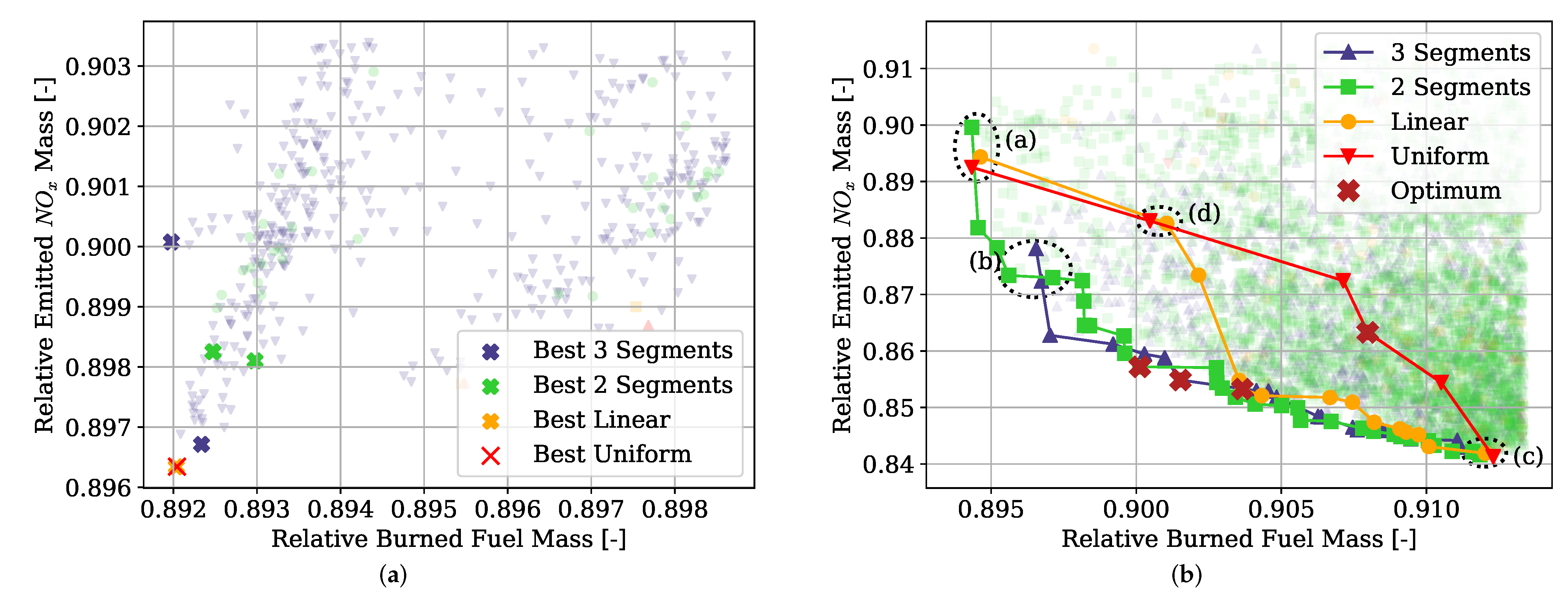
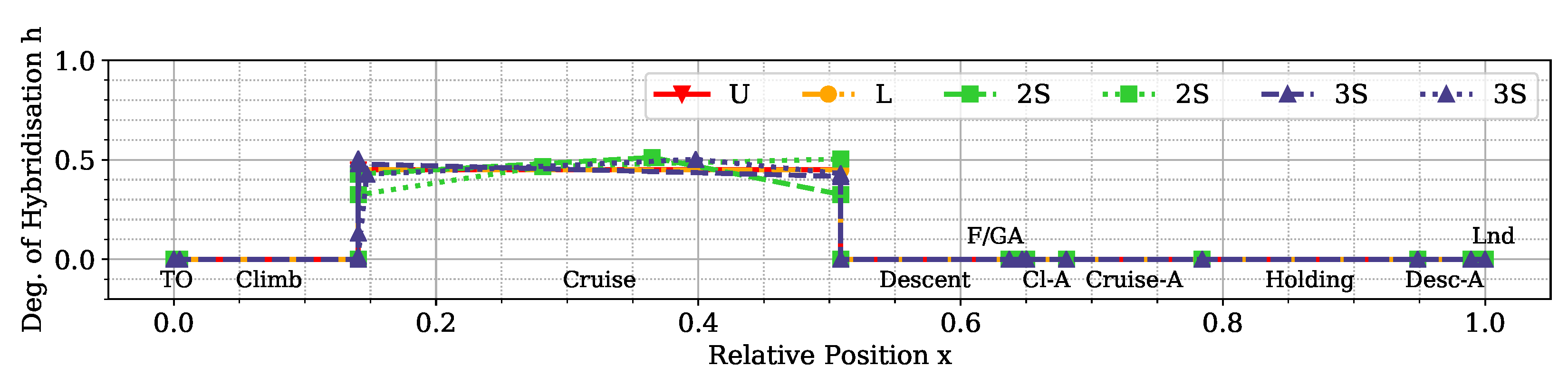
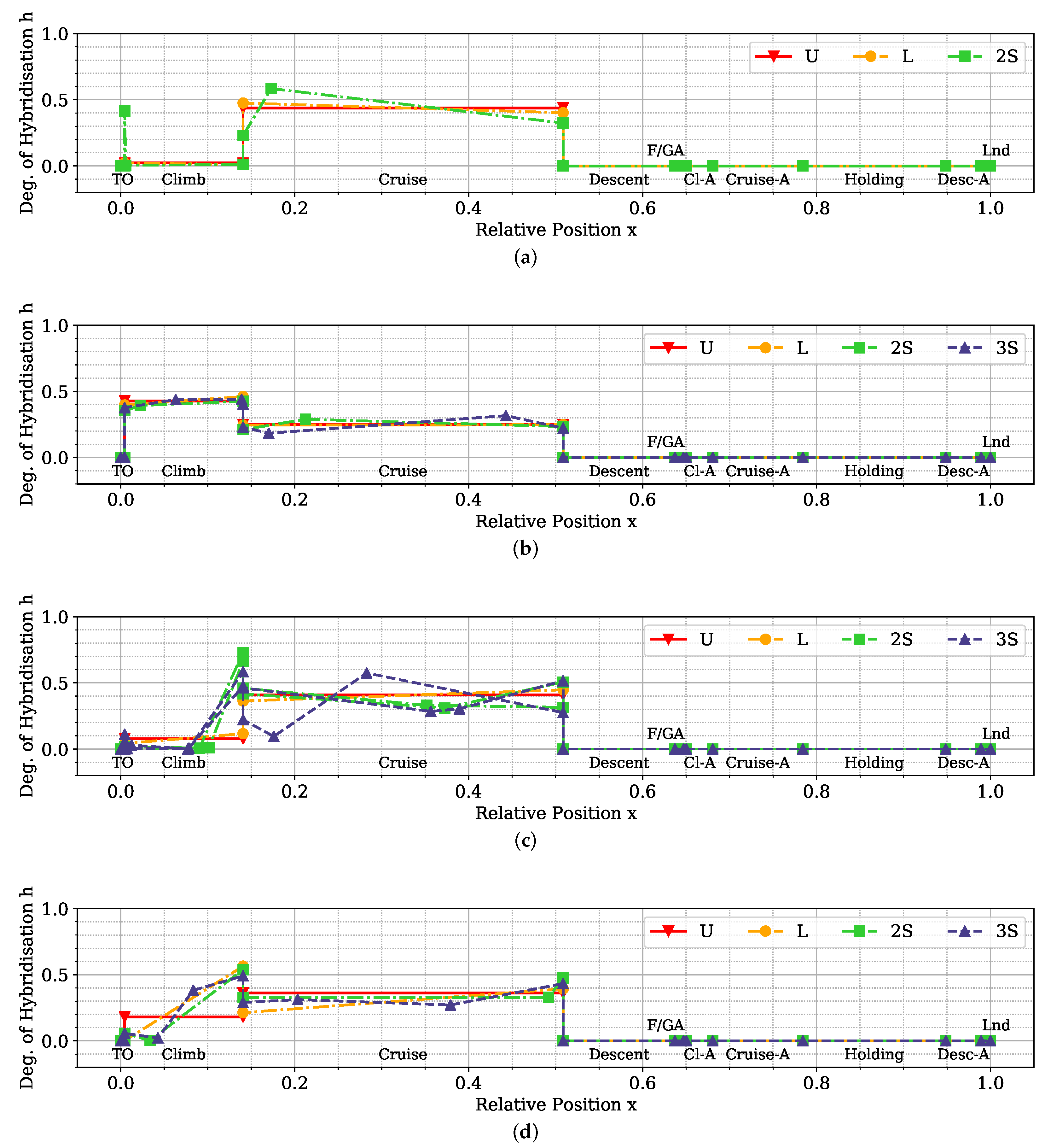
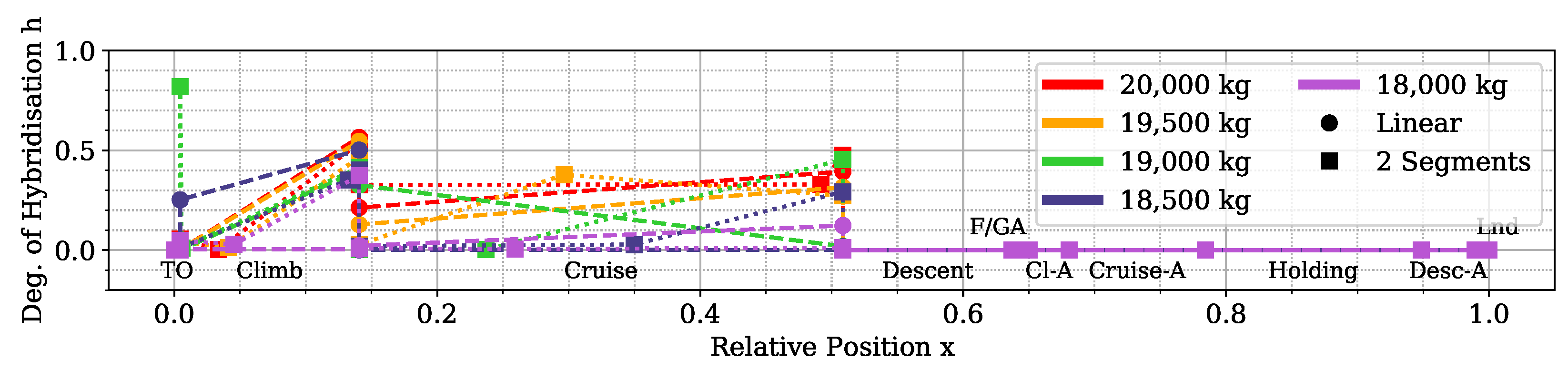
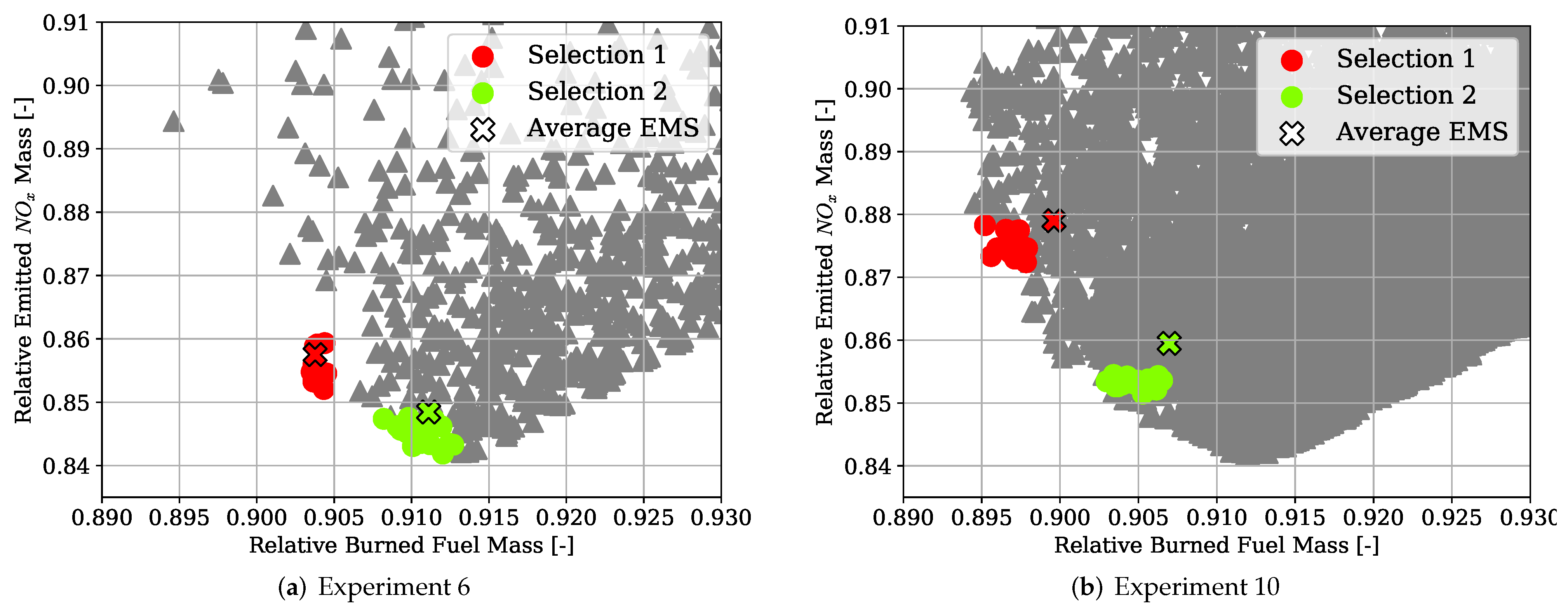
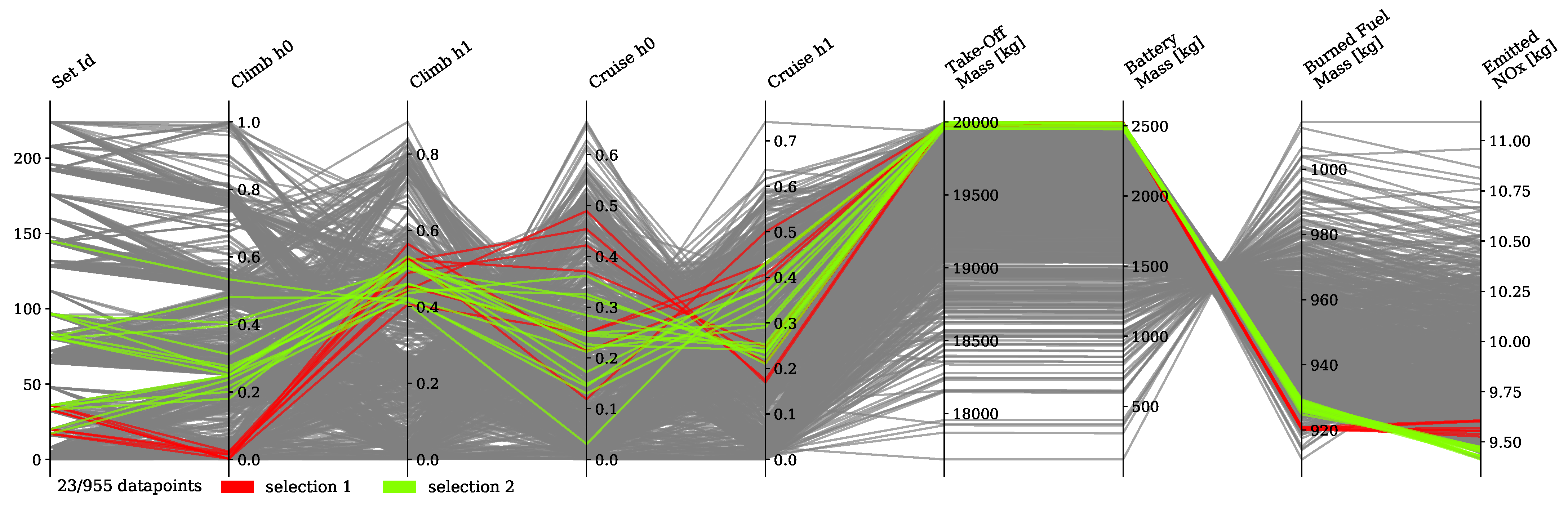
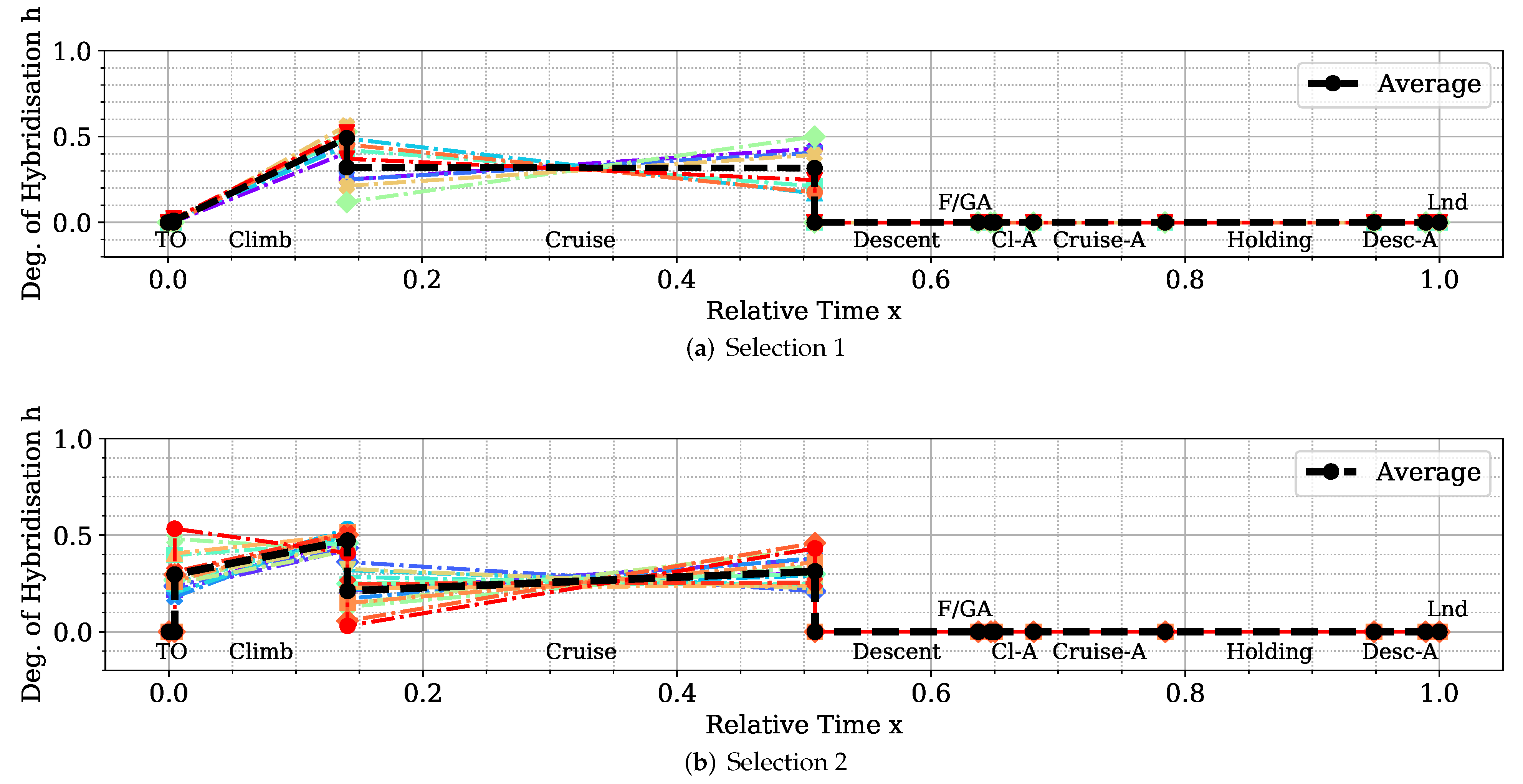
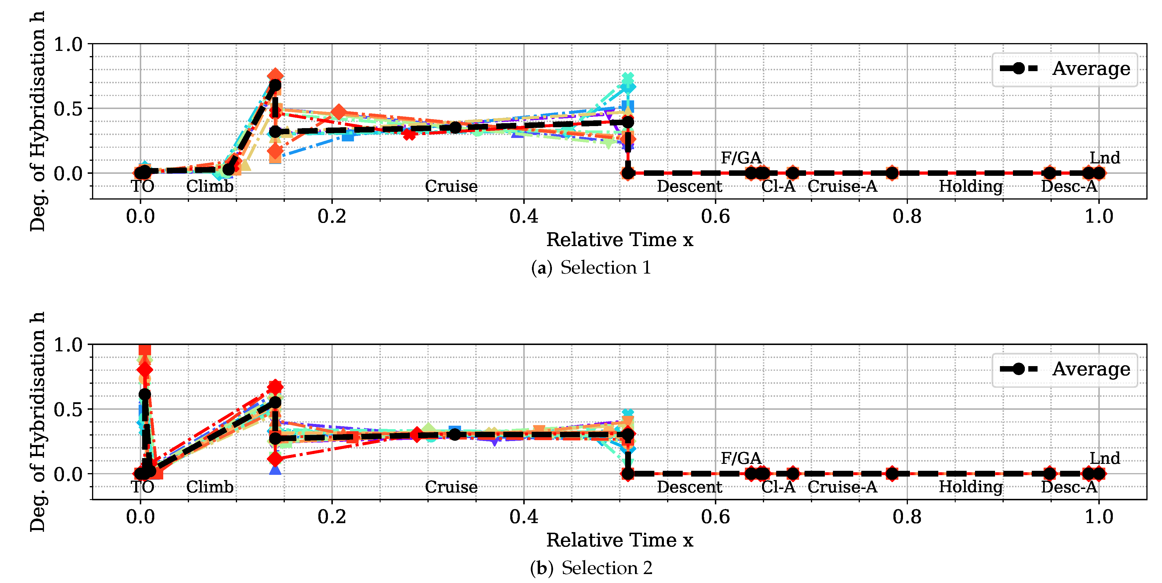
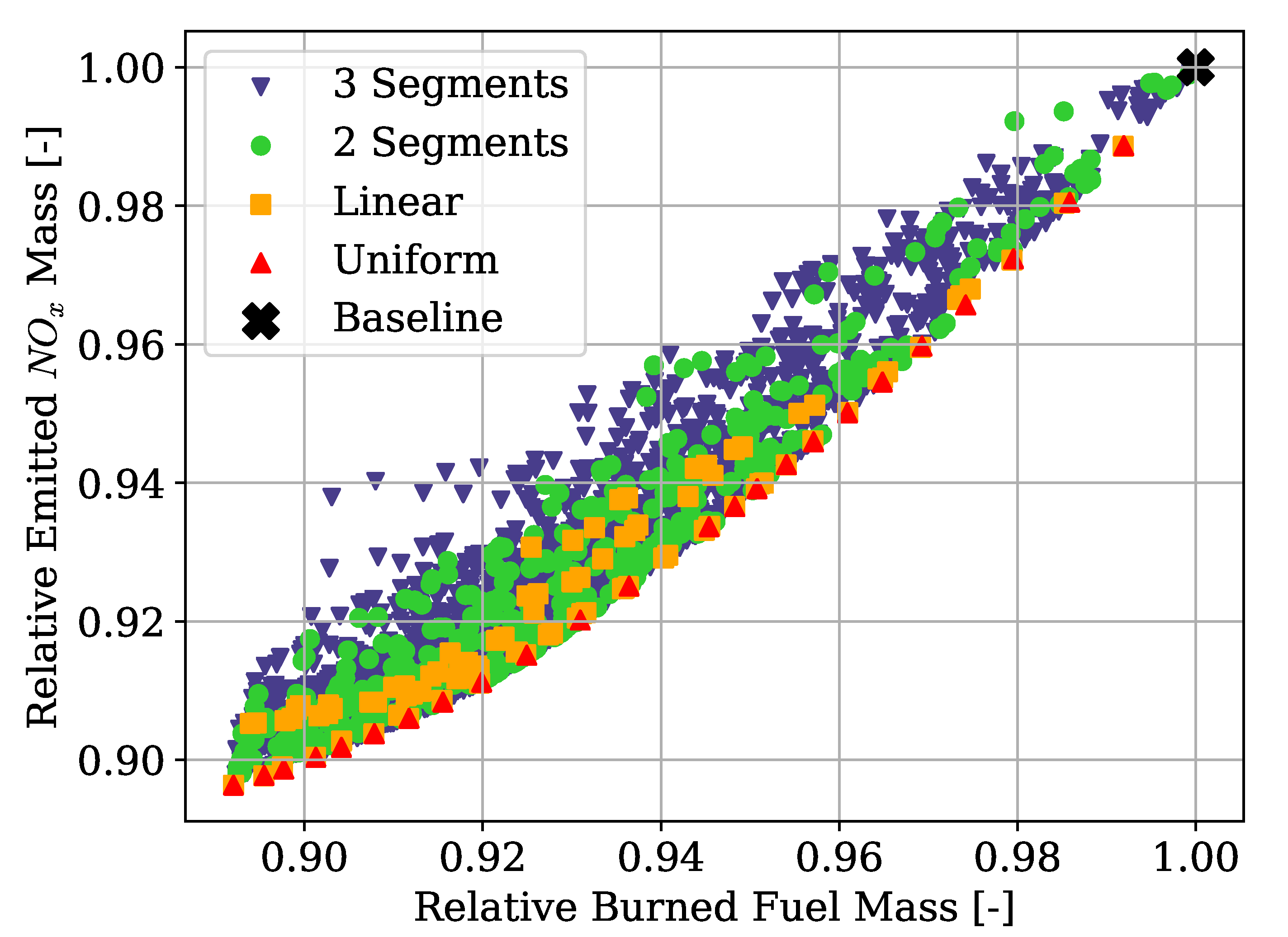
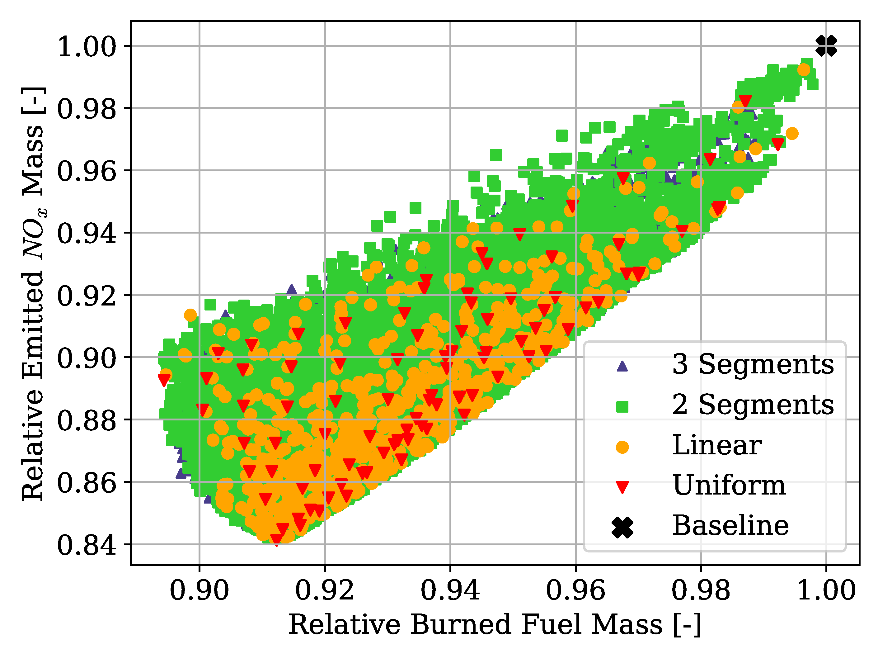
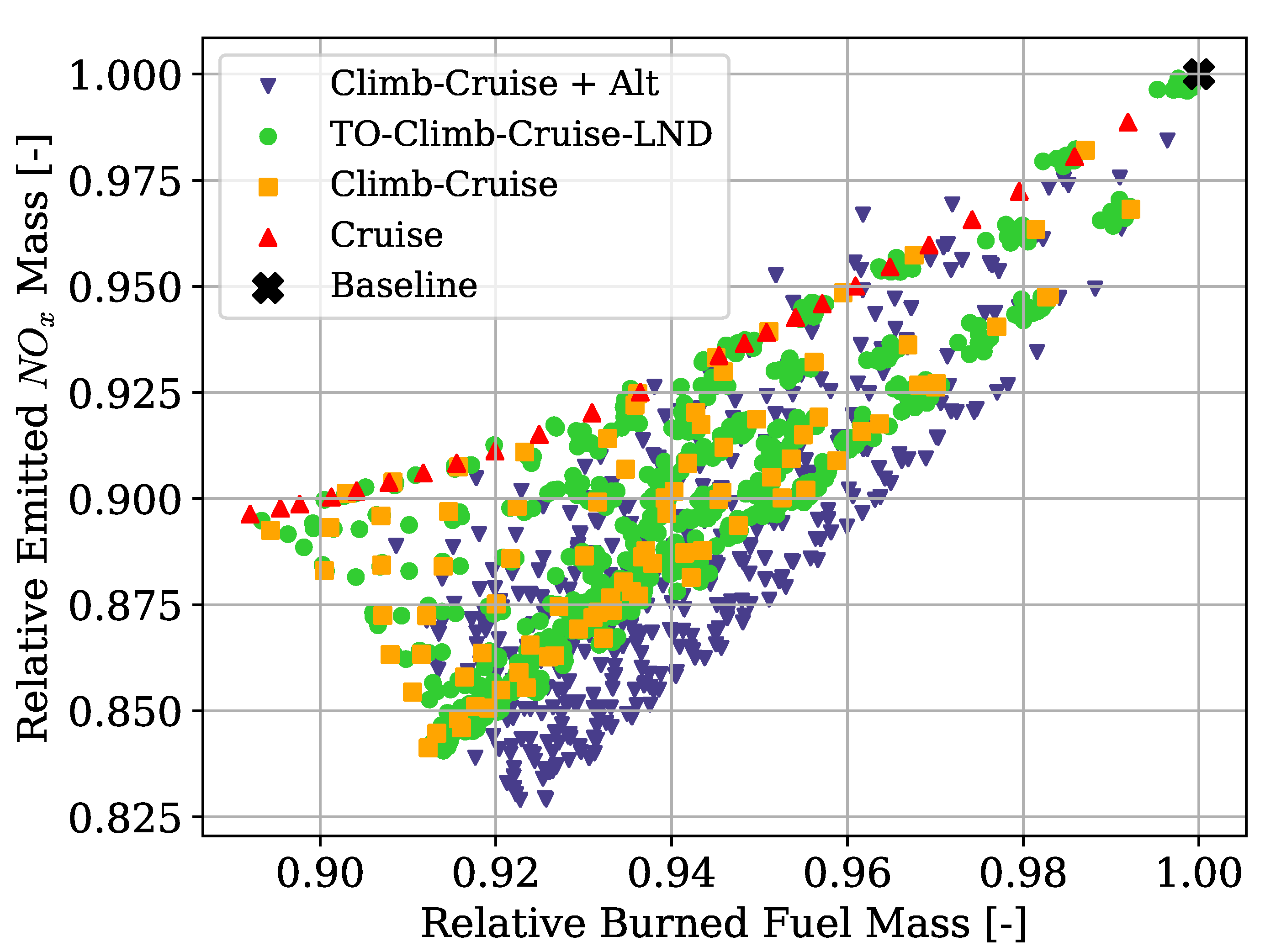
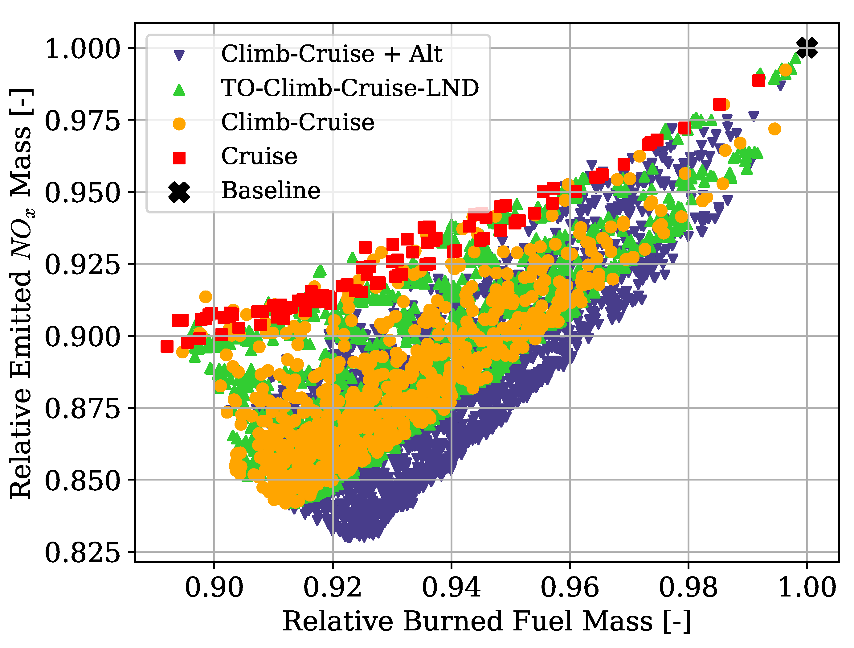
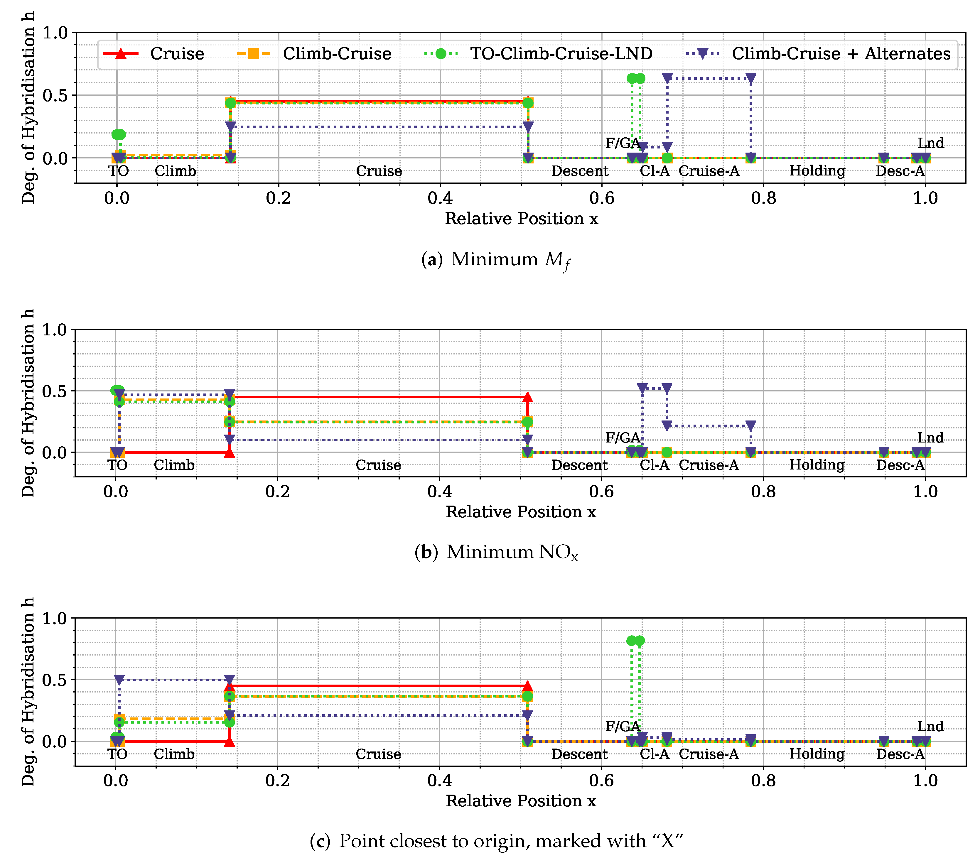
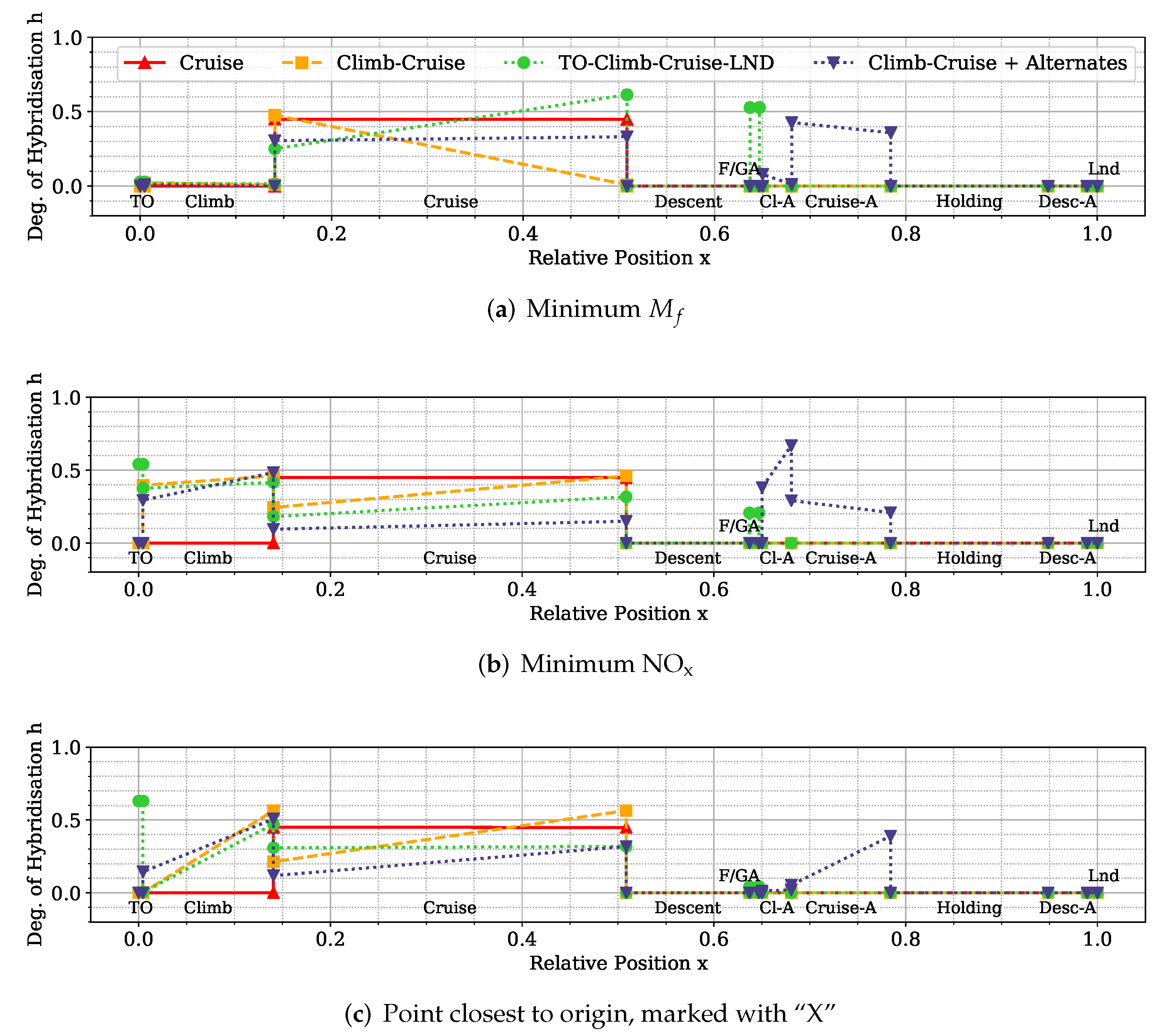
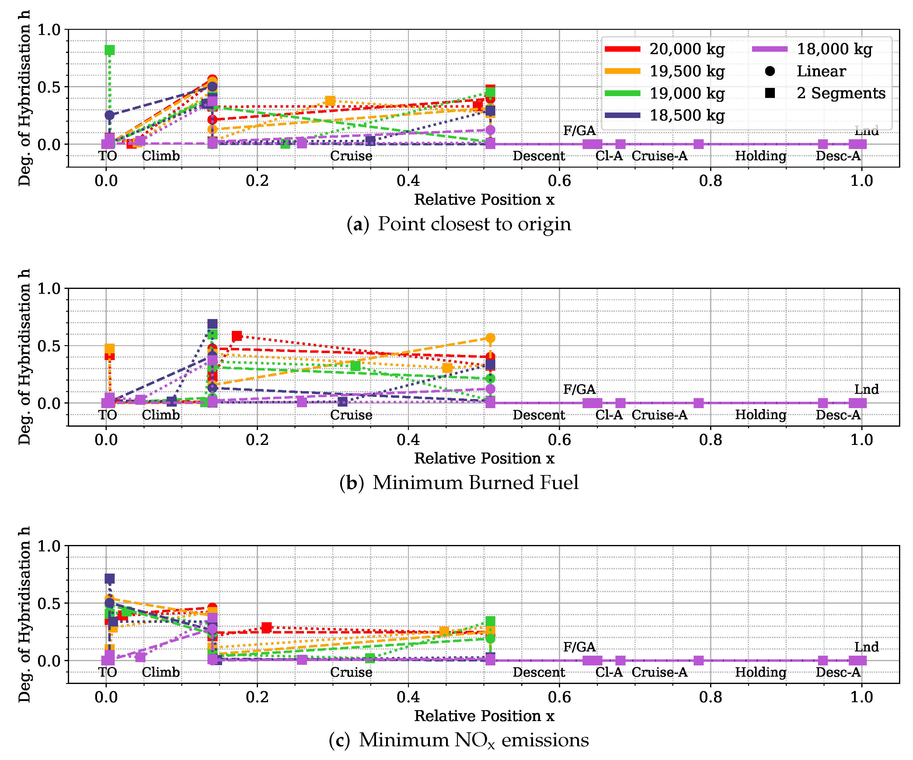
Hybrid-electric vehicles are characterised by providing propulsive power from more than a single energy source. Finding the optimal energy schedule is a common issue that affects hybrid-electric aircraft, albeit with the added complexity of take-off mass limitations. This study presented the problem of finding the optimal energy management scheduling for a hybrid-electric aircraft combined with its battery sizing. An ATR-42 class aircraft retrofitted with a hybrid-electric parallel propulsion system was modelled, and a piecewise linear parametrisation of the degree of hybridisation was introduced for flexibly defining any energy management strategy. A new design space exploration methodology based on the principles of Set-Based Design was introduced, enhanced by a probabilistic approach, which is capable of discarding design subspaces unable to satisfy the requirements set by the designer. This methodology allowed the optimisation algorithm to focus on areas of the design space without constraint violations and, when specified, closer to the global Pareto front. Indeed, the presented test cases had a large portion of the design space unable to satisfy the constraints. The framework was capable of identifying it and discarding it, reducing the number of configurations to evaluate by 75% on average. Furthermore, the optimisation results obtained with this approach allowed us to reveal the behaviour of the system. Nevertheless, a set of tuning hyperparameters of this framework was identified, the granularity of the subspaces and the minimum satisfaction probability, which affect the number of possible results. Tuning studies will be performed to benchmark the proposed methodology and define best practice hyperparameters. Several experiments were performed by changing the complexity of the parametrisation and the number of hybridised mission phases, from which several lessons were learned. The complexity of the energy management parametrisation has diminishing returns on the objectives. The piecewise two-segment topology was found to be enough for identifying the Pareto front. Introducing more phases did not improve the objective significantly to justify the increased computational cost. Furthermore, points in the same area of the objective space have similar energy management strategies, regardless of how complex and flexible their parametrisation is. Indeed, the parametrisation itself was not responsible for the trade-off between the objectives.

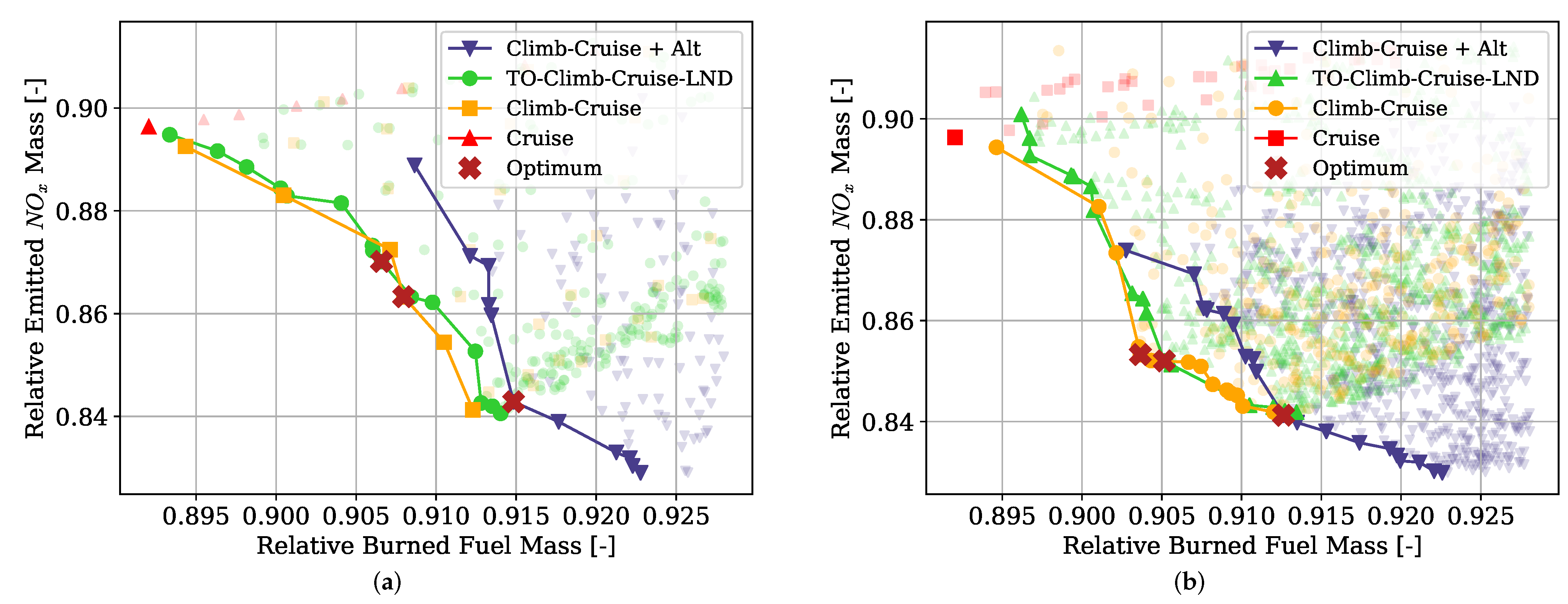
Instead, the length and number of the hybridised mission phases affected the shape and presence of a Pareto front. The results clearly showed that, while the longest mission phases contributed the most to the reduction of fuel consumption, if most mission phases were hybridised, the ${\mathrm{NO}}_{\mathrm{x}}$ emissions would go down together with an increment in the overall propulsive efficiency. Moreover, the maximum take-off mass limit affects how much trade-off is present between the objectives. These phenomena can be explained in the limited amount of available electric energy due to the limited amount of battery mass. If this energy is distributed over more mission phases, on average, less gas turbine power is used, and therefore, less ${\mathrm{NO}}_{\mathrm{x}}$ is emitted as it runs at a lower combustion temperature. However, the DoH would be lower on the longer mission phases, requiring most fuel burned. Indeed, if the electric energy is used only on the longest mission phase, cruise, the mission fuel consumption is minimised.

Lastly, the maximum take-off mass determines how much battery mass is distributed over the mission phases. While this might suggest increasing this limit indefinitely, the increment in the battery mass and the higher amount of electric power to manage would greatly impact the aircraft’s structural and systems mass, increasing the aircraft’s cost and complexity and ultimately reducing the fuel efficiency benefits.

This aspect was not included in this study but will be included in future work. Furthermore, from this study, the thermal management aspect of the hybrid-electric propulsion system was ignored, which is one of the current challenges in the design and production of HEA. Future studies will introduce the sizing of the thermal management system (TMS) from the electric system lost energy and its effects on aircraft mass and available power.

Finally, a critical aspect in the study and development of HE and Electric propulsion is the uncertainty of future technology. In this study, a fixed value of battery energy density was selected for a 2050 scenario. However, future studies will introduce an uncertainty into the presented methodology for studying different technological scenarios and their impact on the design parameters and requirements at the same time.

References

1. European Commission. Flightpath 2050: Europe’s Vision for Aviation-Report of the High Level Group on Aviation Research. In Report of the High Level Group on Aviation Research; European Commission: Luxembourg, 2011; Available online: https://www.acare4europe.org/sites/acare4europe.org/files/document/Flightpath2050_Final.pdf (accessed on 17 November 2021).
2. Zaporozhets, O.; Isaienko, V.; Synylo, K. Trends on Current and Forecasted Aircraft Hybrid Electric Architectures and Their Impact on Environment. Energy 2020, 211, 118814. [Google Scholar] [CrossRef]
3. Brelje, B.J.; Martins, J.R.R.A. Electric, Hybrid, and Turboelectric Fixed-Wing Aircraft: A Review of Concepts, Models, and Design Approaches. Prog. Aerosp. Sci. 2019, 104, 1–19. [Google Scholar] [CrossRef]
4. Sahoo, S.; Zhao, X.; Kyprianidis, K. A Review of Concepts, Benefits, and Challenges for Future Electrical Propulsion-Based Aircraft. Aerospace 2020, 7, 44. [Google Scholar] [CrossRef] [Green Version]
5. Epstein, A.H.; O’Flarity, S.M. Considerations for Reducing Aviation’s CO2 with Aircraft Electric Propulsion. J. Propuls. Power 2019, 35, 572–582. [Google Scholar] [CrossRef]
6. Isikveren, A.T.; Kaiser, S.; Pornet, C.; Vratny, P.C. Pre-Design Strategies and Sizing Techniques for Dual-Energy Aircraft. Aircr. Eng. Aerosp. Technol. 2014, 86, 525–542. [Google Scholar] [CrossRef]
7. Zhang, F.; Wang, L.; Coskun, S.; Pang, H.; Cui, Y.; Xi, J. Energy Management Strategies for Hybrid Electric Vehicles: Review, Classification, Comparison, and Outlook. Energies 2020, 13, 3352. [Google Scholar] [CrossRef]
8. Xie, Y.; Savvarisal, A.; Tsourdos, A.; Zhang, D.; Gu, J. Review of Hybrid Electric Powered Aircraft, Its Conceptual Design and Energy Management Methodologies. Chin. J. Aeronaut. 2021, 34, 432–450. [Google Scholar] [CrossRef]
9. Hung, J.Y.; Gonzalez, L.F. On Parallel Hybrid-Electric Propulsion System for Unmanned Aerial Vehicles. Prog. Aerosp. Sci. 2012, 51, 1–17. [Google Scholar] [CrossRef] [Green Version]
10. Karunarathne, L.; Economou, J.T.; Knowles, K. Adaptive Neuro Fuzzy Inference System-Based Intelligent Power Management Strategies for Fuel Cell/Battery Driven Unmanned Electric Aerial Vehicle. Proc. Inst. Mech. Eng. Part G J. Aerosp. Eng. 2010, 224, 77–88. [Google Scholar] [CrossRef]
11. Pinto Leite, J.P.S.; Voskuijl, M. Optimal Energy Management for Hybrid-Electric Aircraft. Aircr. Eng. Aerosp. Technol. 2020, 92, 851–861. [Google Scholar] [CrossRef]
12. Misley, A.A.; D’Arpino, M.; Ramesh, P.; Canova, M. A Real-Time Energy Management Strategy for Hybrid Electric Aircraft Propulsion Systems. In Proceedings of the AIAA Propulsion and Energy 2021 Forum, Online, 9–12 August 2021; American Institute of Aeronautics and Astronautics: Reston, VA, USA, 2021. [Google Scholar] [CrossRef]
13. Pornet, C.; Gologan, C.; Vratny, P.C.; Seitz, A.; Schmitz, O.; Isikveren, A.T.; Hornung, M. Methodology for Sizing and Performance Assessment of Hybrid Energy Aircraft. J. Aircraft 2015, 52, 341–352. [Google Scholar] [CrossRef]
14. Zamboni, J.; Vos, R.; Emeneth, M.; Schneegans, A. A Method for the Conceptual Design of Hybrid Electric Aircraft. In Proceedings of the AIAA Scitech 2019 Forum, San Diego, CA, USA, 7–11 January 2019; American Institute of Aeronautics and Astronautics: Reston, VA, USA, 2019. [Google Scholar] [CrossRef] [Green Version]
15. Trawick, D.R. A Methodology for the Determination of Optimal Operational Schedules of Hybrid Electric Architectures; Georgia Institute of Technology: Atlanta, GA, USA, 2018. [Google Scholar]
16. Trainelli, L.; Salucci, F.; Rossi, N.; Riboldi, C.E.D.; Rolando, A. Preliminary Sizing and Energy Management of Serial Hybrid-Electric. In Proceedings of the XXV AIDAA National Congress, Italian Association of Aeronautics and Astronautics, Rome, Italy, 9–12 September 2019. [Google Scholar]
17. Bradley, M.K.; Droney, C.K. Subsonic Ultra Green Aircraft Research: Phase 2—Volume II— Hybrid Electric Design Exploration; NASA Langely Research Center: Hampton, VA, USA, 2015.
18. Lents, C.E.; Hardin, L.W.; Rheaume, J.; Kohlman, L. Parallel Hybrid Gas-Electric Geared Turbofan Engine Conceptual Design and Benefits Analysis. In Proceedings of the 52nd AIAA/SAE/ASEE Joint Propulsion Conference, Salt Lake City, UT, USA, 25–27 July 2016; American Institute of Aeronautics and Astronautics: Reston, VA, USA, 2016. [Google Scholar] [CrossRef] [Green Version]
19. Lents, C.E.; Hardin, L.W. Fuel Burn and Energy Consumption Reductions of a Single-Aisle Class Parallel Hybrid Propulsion System. In Proceedings of the AIAA Propulsion and Energy 2019 Forum, Indianapolis, IN, USA, 22–24 August 2019; American Institute of Aeronautics and Astronautics: Reston, VA, USA, 2019. [Google Scholar] [CrossRef]
20. Rheaume, J.M.; MacDonald, M.; Lents, C.E. Commercial Hybrid Electric Aircraft Thermal Management System Design, Simulation, and Operation Improvements. In Proceedings of the AIAA Propulsion and Energy 2019 Forum, Indianapolis, IN, USA, 22–24 August 2019; American Institute of Aeronautics and Astronautics: Reston, VA, USA, 2019. [Google Scholar] [CrossRef]
21. Trawick, D.; Perullo, C.; Armstrong, M.; Snyder, D.; Tai, J.C.; Mavris, D.N. Development and Application of GT-HEAT for the Electrically Variable Engine(TM) Design. In Proceedings of the 55th AIAA Aerospace Sciences Meeting, Grapevine, TX, USA, 9–13 January 2017; American Institute of Aeronautics and Astronautics: Reston, VA, USA, 2017. [Google Scholar] [CrossRef]
22. Gladin, J.C.; Trawick, D.; Mavris, D.N.; Armstrong, M.J.; Bevis, D.; Klein, K. Fundamentals of Parallel Hybrid Turbofan Mission Analysis with Application to the Electrically Variable Engine. In Proceedings of the 2018 AIAA/IEEE Electric Aircraft Technologies Symposium, Cincinnati, OH, USA, 12–14 July 2018; American Institute of Aeronautics and Astronautics: Reston, VA, USA, 2018. [Google Scholar] [CrossRef]
23. Perullo, C.; Trawick, D.; Armstrong, M.; Tai, J.C.; Mavris, D.N. Cycle Selection and Sizing of a Single-Aisle Transport with the Electrically Variable Engine(TM) (EVE) for Fleet Level Fuel Optimization. In Proceedings of the 55th AIAA Aerospace Sciences Meeting, Grapevine, TX, USA, 9–13 January 2017; American Institute of Aeronautics and Astronautics: Reston, VA, USA, 2017. [Google Scholar] [CrossRef]
24. Pornet, C.; Kaiser, S.; Isikveren, A.T.; Hornung, M. Integrated Fuel-Battery Hybrid for a Narrow-Body Sized Transport Aircraft. Aircr. Eng. Aerosp. Technol. Int. J. 2014, 86, 568–574. [Google Scholar] [CrossRef]
25. Xin, Z.; Sahoo, S.; Kyprianidis, K.; Sumsurooah, S.; Valente, G.; Rashed, M.; Vakil, G.; Hill, C.I.; Jacob, C.; Gobbin, A. A Framework for Optimization of Hybrid Aircraft. In Proceedings of the ASME Turbo Expo 2019: Turbomachinery Technical Conference and Exposition, Phoenix, AZ, USA, 17–21 June 2019; American Society of Mechanical Engineers (ASME): New York, NY, USA, 2019; Volume 3. [Google Scholar] [CrossRef]
26. Nunez, M.; Datta, V.C.; Molina-Cristobal, A.; Guenov, M.; Riaz, A. Enabling Exploration in the Conceptual Design and Optimisation of Complex Systems. J. Eng. Des. 2012, 23, 852–875. [Google Scholar] [CrossRef]
27. Ullman, D.G. The Mechanical Design Process; David Ullman LLC: Independence, OR, USA, 2017; ISBN 978-0-387-21507-5. [Google Scholar]
28. Pahl, G.; Beitz, W.; Feldhussen, J.; Karl-Heinrich, G. Engineering Design. A Systematic Approach; Springer: London, UK, 2007; ISBN 978-1-4471-6025-0. [Google Scholar]
29. Brahma, A.; Wynn, D.C. Margin Value Method for Engineering Design Improvement. Res. Eng. Design 2020, 31, 353–381. [Google Scholar] [CrossRef]
30. Guenov, M.D.; Chen, X.; Molina-Cristóbal, A.; Riaz, A.; van Heerden, A.S.J.; Padulo, M. Margin Allocation and Tradeoff in Complex Systems Design and Optimization. AIAA J. 2018, 56, 2887–2902. [Google Scholar] [CrossRef] [Green Version]
31. Pugh, S. Total Design: Integrated Methods for Successful Product Engineering; Prentice Hall: Wokingham, UK, 1990; ISBN 978-0-201-41639-8. [Google Scholar]
32. Wheelwright, S.C.; Clark, K.B. Revolutionizing Product Development: Quantum Leaps in Speed, Efficiency, and Quality; Simon and Schuster: New York, NY, USA, 1992; ISBN 978-0-02-905515-1. [Google Scholar]
33. Sobek II, D.; Ward, A.; Liker, J. Toyota’s Principles of Set-Based Concurrent Engineering. MIT Sloan Manag. Rev. 1999, 40, 67–83. [Google Scholar]
34. Singer, D.J.; Doerry, N.; Buckley, M.E. What Is Set-Based Design? Naval Eng. J. 2009, 121, 31–43. [Google Scholar] [CrossRef]
35. Shallcross, N.; Parnell, G.S.; Pohl, E.; Specking, E. Set-Based Design: The State-of-Practice and Research Opportunities. Syst. Eng. 2020, 23, 1–22. [Google Scholar] [CrossRef]
36. Small, C.; Parnell, G.S.; Pohl, E.; Goerger, S.R.; Cilli, M.; Specking, E. Demonstrating Set-Based Design Techniques: An Unmanned Aerial Vehicle Case Study. J. Def. Model. Simul. 2020, 17, 339–355. [Google Scholar] [CrossRef]
37. Al Handawi, K.; Andersson, P.; Panarotto, M.; Isaksson, O.; Kokkolaras, M. Scalable Set-Based Design Optimization and Remanufacturing for Meeting Changing Requirements. J. Mech. Des. 2020, 143, 21702. [Google Scholar] [CrossRef]
38. Inoue, M.; Suzuki, W.; Yamada, S.; Aoyama, K. A Universal Design Method That Considers Variability in User Requirements: A Case Study of Mechanical Pencil Design. J. Adv. Mech. Des. Syst. Manuf. 2021, 15, JAMDSM0022. [Google Scholar] [CrossRef]
39. Wade, Z.; Parnell, G.S.; Goerger, S.R.; Pohl, E.; Specking, E. Designing Engineered Resilient Systems Using Set-Based Design. In Proceedings of the Systems Engineering in Context; Adams, S., Beling, P.A., Lambert, J.H., Scherer, W.T., Fleming, C.H., Eds.; Springer International Publishing: Cham, Switzerland, 2019; pp. 111–122. [Google Scholar] [CrossRef]
40. Specking, E.; Shallcross, N.; Parnell, G.S.; Pohl, E. Quantitative Set-Based Design to Inform Design Teams. Appl. Sci. 2021, 11, 1239. [Google Scholar] [CrossRef]
41. Shallcross, N.J.; Parnell, G.S.; Pohl, E.; Goerger, S.R. A Value of Information Methodology for Multiobjective Decisions in Quantitative Set-Based Design. Syst. Eng. 2021, 24, 409–424. [Google Scholar] [CrossRef]
42. Shallcross, N.J.; Parnell, G.S.; Pohl, E.; Goerger, S.R. Using Value of Information in Quantitative Set-Based Design. Syst. Eng. 2021, 24, 439–455. [Google Scholar] [CrossRef]
43. Avigad, G.; Moshaiov, A. Set-Based Concept Selection in Multi-Objective Problems Involving Delayed Decisions. J. Eng. Des. 2010, 21, 619–646. [Google Scholar] [CrossRef]
44. Gong, D.; Sun, J.; Miao, Z. A Set-Based Genetic Algorithm for Interval Many-Objective Optimization Problems. IEEE Trans. Evol. Comput. 2018, 22, 47–60. [Google Scholar] [CrossRef]
45. Moshaiov, A.; Snir, A.; Samina, B. Concept-Based Evolutionary Exploration of Design Spaces by a Resolution-Relaxation-Pareto Approach. In Proceedings of the 2015 IEEE Congress on Evolutionary Computation (CEC), Sendai, Japan, 25–28 May 2015; pp. 1845–1852. [Google Scholar] [CrossRef]
46. Veenhuis, C.B. A Set-Based Particle Swarm Optimization Method. In Proceedings of the Parallel Problem Solving from Nature—PPSN X; Rudolph, G., Jansen, T., Beume, N., Lucas, S., Poloni, C., Eds.; Springer: Berlin/Heidelberg, Germany, 2008; pp. 971–980. [Google Scholar] [CrossRef]
47. Parker, R.R.; Malak, R.J., Jr. Technology Characterization Models and Their Use in Designing Complex Systems. In Proceedings of the ASME Design Engineering Technical Conference, Washington, DC, USA, 28–31 August 2011; pp. 1063–1075. [Google Scholar] [CrossRef] [Green Version]
48. Hannapel, S.; Vlahopoulos, N. Implementation of Set-Based Design in Multidisciplinary Design Optimization. Struct. Multidisc. Optim. 2014, 50, 101–112. [Google Scholar] [CrossRef]
49. Georgiades, A.; Sharma, S.; Kipouros, T.; Savill, M. ADOPT: An Augmented Set-Based Design Framework with Optimisation. Des. Sci. 2019, 5, e4. [Google Scholar] [CrossRef] [Green Version]
50. Finch, W.W.; Ward, A.C. A Set-Based System for Eliminating Infeasible Designs. In Proceedings of the ASME 1997 Design Engineering Technical Conferences, Sacramento, CA, USA, 14–17 September 1997; American Society of Mechanical Engineers: New York, NY, USA, 1997. [Google Scholar] [CrossRef]
51. Yannou, B.; Yvars, P.-A.; Hoyle, C.; Chen, W. Set-Based Design by Simulation of Usage Scenario Coverage. J. Eng. Des. 2013, 24, 575–603. [Google Scholar] [CrossRef] [Green Version]
52. Venter, G.; Haftka, R.T. Using Response Surface Approximations in Fuzzy Set Based Design Optimization. Struct. Optim. 1999, 18, 218–227. [Google Scholar] [CrossRef]
53. Shahan, D.W.; Seepersad, C.C. Bayesian Network Classifiers for Set-Based Collaborative Design. J. Mech. Design 2012, 134. [Google Scholar] [CrossRef] [Green Version]
54. Han, H.; Chang, S.; Kim, H. Multiple Target Exploration Approach for Design Exploration Using a Swarm Intelligence and Clustering. J. Mech. Des. 2019, 141, 091401. [Google Scholar] [CrossRef] [Green Version]
55. Miller, S.W.; Yukish, M.A.; Simpson, T.W. Design as a Sequential Decision Process. Struct. Multidisc. Optim. 2018, 57, 305–324. [Google Scholar] [CrossRef]
56. Chhabra, J.P.S.; Warn, G.P. A Method for Model Selection Using Reinforcement Learning When Viewing Design as a Sequential Decision Process. Struct. Multidisc. Optim. 2019, 59, 1521–1542. [Google Scholar] [CrossRef]
57. Rasmussen, C.E.; Williams, C.K.I. Gaussian Processes for Machine Learning; Adaptive Computation and Machine Learning Series; MIT Press: Cambridge, MA, USA, 2005; ISBN 978-0-262-18253-9. [Google Scholar]
58. Spinelli, A.; Anderson, L.; Enalou, H.B.; Zaghari, B.; Kipouros, T.; Laskaridis, P. Application of Probabilistic Principles to Set-Based Design for the Optimisation of a Hybrid-Electric Propulsion System. IOP Conf. Ser. Mater. Sci. Eng. 2022, 1226, 12064. [Google Scholar] [CrossRef]
59. Smith, R.C. Uncertainty Quantification: Theory, Implementation, and Applications; SIAM: Philadelphia, PA, USA, 2013; ISBN 978-1-61197-321-1. [Google Scholar]
60. Cunha, A.; Nasser, R.; Sampaio, R.; Lopes, H.; Breitman, K. Uncertainty Quantification through the Monte Carlo Method in a Cloud Computing Setting. Comput. Phys. Commun. 2014, 185, 1355–1363. [Google Scholar] [CrossRef] [Green Version]
61. Yao, W.; Chen, X.; Luo, W.; van Tooren, M.; Guo, J. Review of Uncertainty-Based Multidisciplinary Design Optimization Methods for Aerospace Vehicles. Prog. Aerosp. Sci. 2011, 47, 450–479. [Google Scholar] [CrossRef]
62. Palar, P.S.; Zuhal, L.R.; Shimoyama, K.; Tsuchiya, T. Global Sensitivity Analysis via Multi-Fidelity Polynomial Chaos Expansion. Reliab. Eng. Syst. Saf. 2018, 170, 175–190. [Google Scholar] [CrossRef] [Green Version]
63. Bianchi, D.H.B.D.; Sêcco, N.R.; Silvestre, F.J. A Framework for Enhanced Decision-Making in Aircraft Conceptual Design Optimisation under Uncertainty. Aeronaut. J. 2021, 125, 777–806. [Google Scholar] [CrossRef]
64. Oliver, M.A.; Webster, R. Kriging: A Method of Interpolation for Geographical Information Systems. Int. J. Geogr. Inf. Sys. 1990, 4, 313–332. [Google Scholar] [CrossRef]
65. Pedregosa, F.; Varoquaux, G.; Gramfort, A.; Michel, V.; Thirion, B.; Grisel, O.; Blondel, M.; Prettenhofer, P.; Weiss, R.; Dubourg, V.; et al. Scikit-Learn: Machine Learning in Python. J. Mach. Learn. Res. 2011, 12, 2825–2830. [Google Scholar]
66. Helton, J.C.; Davis, F.J. Latin Hypercube Sampling and the Propagation of Uncertainty in Analyses of Complex Systems. Reliab. Eng. Syst. Saf. 2003, 81, 23–69. [Google Scholar] [CrossRef] [Green Version]
67. Blank, J.; Deb, K. Pymoo: Multi-Objective Optimization in Python. IEEE Access 2020, 8, 89497–89509. [Google Scholar] [CrossRef]
68. Seada, H.; Deb, K. A Unified Evolutionary Optimization Procedure for Single, Multiple, and Many Objectives. IEEE Trans. Evol. Comput. 2016, 20, 358–369. [Google Scholar] [CrossRef]
69. Regis, R.G. Particle Swarm with Radial Basis Function Surrogates for Expensive Black-Box Optimization. J. Comput. Sci. 2014, 5, 12–23. [Google Scholar] [CrossRef]
70. Pagliuca, G.; Kipouros, T.; Savill, M.A. Surrogate Modelling for Wing Planform Multidisciplinary Optimisation Using Model-Based Engineering. Int. J. Aerosp. Eng. 2019, 2019, e4327481. [Google Scholar] [CrossRef]
71. Inselberg, A. Parallel Coordinates: Visual Multidimensional Geometry and Its Applications; Springer: New York, NY, USA, 2009; ISBN 978-0-387-21507-5. [Google Scholar]
72. Kipouros, T.; Inselberg, A.; Parks, G.; Savill, A.M. Parallel Coordinates in Computational Engineering Design. In Proceedings of the 54th AIAA/ASME/ASCE/AHS/ASC Structures, Structural Dynamics, and Materials Conference, Boston, MA, USA, 8–11 April 2013; American Institute of Aeronautics and Astronautics: Reston, VA, USA, 2013. [Google Scholar] [CrossRef]
73. Nikolaidis, T.; Jafari, S.; Bosak, D.; Pilidis, P. Exchange Rate Analysis for Ultra High Bypass Ratio Geared Turbofan Engines. Appl. Sci. 2020, 10, 7945. [Google Scholar] [CrossRef]
74. DuBois, D.; Paynter, G. Fuel Flow Method2 for Estimating Aircraft Emissions. SAE Trans. J. Aerosp. 2006, 115, 1–14. [Google Scholar] [CrossRef]
75. Filippone, A.; Bojdo, N. Statistical Model for Gas Turbine Engines Exhaust Emissions. Transp. Res. Part Transp. Environ. 2018, 59, 451–463. [Google Scholar] [CrossRef] [Green Version]
76. ATR-42-600 Factsheet. Available online: https://www.atr-aircraft.com/wp-content/uploads/2020/07/Factsheets_-_ATR_42-600.pdf (accessed on 21 February 2022).
77. Eisenhut, D.; Moebs, N.; Windels, E.; Bergmann, D.; Geiß, I.; Reis, R.; Strohmayer, A. Aircraft Requirements for Sustainable Regional Aviation. Aerospace 2021, 8, 61. [Google Scholar] [CrossRef]
78. Edström, K.; Dominko, R.; Fichtner, M.; Otuszewski, T.; Perraud, S.; Punckt, C.; Tarascon, J.-M.; Vegge, T.; Winter, M.; Dominko, R. BATTERY 2030+ Roadmap. 2020. Available online: https://battery2030.eu/wp-content/uploads/2021/08/c_860904-l_1-k_roadmap-27-march.pdf (accessed on 7 December 2021).
79. Ojeda-Rodríguez, Á.; González-Vizuete, P.; Bernal-Méndez, J.; Martín-Prats, M.A. A Survey on Bidirectional DC/DC Power Converter Topologies for the Future Hybrid and All Electric Aircrafts. Energies 2020, 13, 4883. [Google Scholar] [CrossRef]
80. Sirimanna, S.; Thanatheepan, B.; Lee, D.; Agrawal, S.; Yu, Y.; Wang, Y.; Anderson, A.; Banerjee, A.; Haran, K. Comparison of Electrified Aircraft Propulsion Drive Systems with Different Electric Motor Topologies. J. Propuls. Power 2021, 37, 733–747. [Google Scholar] [CrossRef]
81. Wulff, A.; Hourmouziadis, J. Technology Review of Aeroengine Pollutant Emissions. Aerosp. Sci. Technol. 1997, 1, 557–572. [Google Scholar] [CrossRef]
Figure 1. Flowchart of the proposed methodology.
Aerospace 09 00147 g001
Figure 2. Flowchart of the exploration step.
Aerospace 09 00147 g002
Figure 3. Examples of energy management definitions over a single mission phase.
Aerospace 09 00147 g003
Figure 4. Mission Profile.
Aerospace 09 00147 g004
Figure 5. Propulsion system configuration.
Aerospace 09 00147 g005
Figure 6. Data of Experiment CC-2S.
Aerospace 09 00147 g006
Figure 7. Data of Experiment CC-2S with additional soft constraints.
Aerospace 09 00147 g007
Figure 8. Objective space of data from Figure 6 and Figure 7.
Aerospace 09 00147 g008
Figure 9. Effects of parametrisation complexity: (a) Optimal points Objective space of cruise-only hybridised strategies; (b) Pareto fronts of climb and cruise hybridisation strategies.
Aerospace 09 00147 g009
Figure 10. Hybridisation strategies of the optimal points of Figure 9a.
Aerospace 09 00147 g010
Figure 11. Optimal energy management strategies of Figure 9b: (a) Selection a; (b) Selection c; (c) Selections b and d; (d) Point closest to origin, marked with “X” in Figure 9b.
Aerospace 09 00147 g011
Figure 12. Effects of mission hybridisation: (a) Pareto fronts of uniform strategies with different hybridised mission phases; (b) Pareto fronts of linear strategies with different hybridised mission phases.
Aerospace 09 00147 g012
Figure 13. Pareto fronts for different Take-off Mass constraints.
Aerospace 09 00147 g013
Figure 14. Energy management strategies for different take-off mass constraint levels.
Aerospace 09 00147 g014
Figure 15. Points selected for the recommended strategies.
Aerospace 09 00147 g015
Figure 16. Parallel coordinates visualisation of Experiment 6.
Aerospace 09 00147 g016
Figure 17. Parallel coordinates visualisation of Experiment 10.
Aerospace 09 00147 g017
Figure 18. Visualisation of Experiment 6 energy management strategies.
Aerospace 09 00147 g018
Figure 19. Visualisation of Experiment 10 energy management strategies.
Aerospace 09 00147 g019