1. Introduction
Although reaching production only in rare instances, three-surface aircraft have been accurately studied, especially in comparison to more traditional configurations. Existing technical works on the matter are typically centered on aerodynamics, such as [
1,
2,
3,
4], structural or aero-elastic performance [
5,
6]. They invariably show that a three-surface aircraft is indeed feasible, while of course implying the need for some more sophistication in aerodynamic and structural design, with respect to more standard configurations. In particular, difficulty in the design and performance prediction is due to the interaction between the canard and the wing. This interaction is not limited to the wake effect of the canard on the wing, but also on the upwash effect of the wing on the canard. For high performance aircraft in canard or three-surface configurations (typically fighters), a close aerodynamic coupling between surfaces prevents the use of standard design and performance prediction techniques, thus complicating the assessment of advantages with respect to more traditional configurations at a preliminary design level. Actually, in those cases the mutual interaction among surfaces is such that the overall airflow cannot be considered as the perturbed result of a superimposition of those pertaining to each isolated surface, so that a preliminary characterization can typically be attempted only via CFD or wind tunnel testing. However, for larger (passenger) aircraft featuring a longer fuselage allowing for an increased longitudinal distance between aerodynamic surfaces, the latter can be treated as aerodynamically decoupled, allowing one to deploy easier predictive models [
1,
2,
3,
4,
7], so as to capture and assess potential pros and cons early in the design process (see
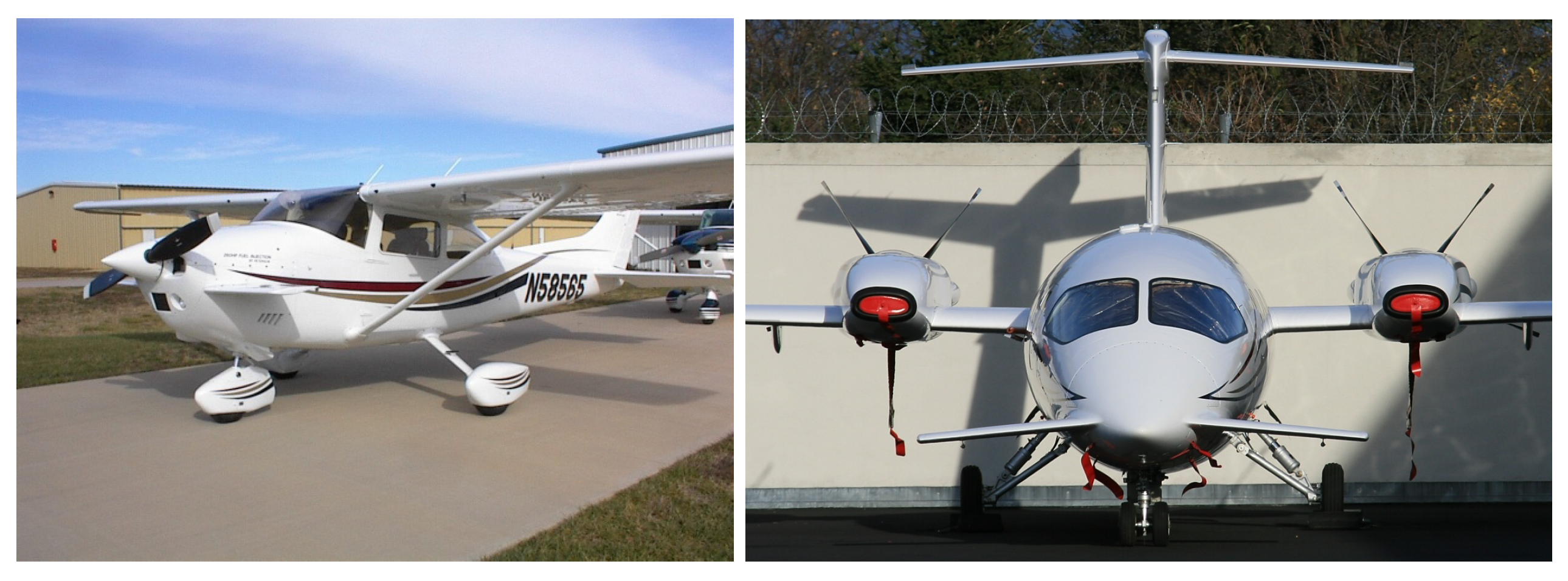
Figure 1 for example designs).
Despite the chance of reducing trim drag being one of the major drivers pushing the three-surface configuration, flight performance and dynamics of this type of aircraft have been superficially investigated in technical works [
7,
8]. A systematic study of flight performance for aircraft with this configuration has been presented only recently in [
9].
Albeit limited to the longitudinal plane, the latter introduces a complete flight dynamics model of a three-surface aircraft, including a control surface for both canard and horizontal tail and accounting for the mutual aerodynamic interactions of surfaces in a loosely coupled geometry. The presence of two movable surfaces entails a redundancy in the longitudinal control of the airplane, which was exploited to minimize the trim drag, i.e., to find the combination of the motion of the two aforementioned surfaces associated to the minimum drag in cruise for any speed and altitude (and, hence, any lift coefficient). As a matter of fact, this possibility is one of the major reasons for adopting a three-surface configuration. Clearly, such an approach cannot be featured by a standard two-surface airplane, which can only be optimized for a single lift coefficient. In addition to investigating this effect, the same cited work simultaneously shows how flying qualities are not degraded on the novel three-surface configuration, nor an increase in pilot’s workload is expected on a three-surface aircraft with respect to a traditional one. These evidence definitely support that a three-surface configuration would be highly desirable in the design framework now faced especially by general aviation, where new designs are much constrained by energy performance [
10,
11,
12,
13,
14].
Figure 1.
Examples of existing three-surface aircraft. (
Left): Wren 460 [
15]. (
Right): Piaggio P180 EVO [
16].
Figure 1.
Examples of existing three-surface aircraft. (
Left): Wren 460 [
15]. (
Right): Piaggio P180 EVO [
16].
Following in the same line, the present paper further explores the potential of three-surface configuration, by moving on to terminal maneuvers, and specifically to take-off. It is self-evident that improving take-off distance is associated to a higher level of safety during terminal conditions. Moreover, since a lower take-off distance would reduce the time spent by the aircraft close to the ground, and consequently its footprint in terms of noise and chemical pollution [
17], an increase in take-off performance would provide another relevant potential advantage in today’s aircraft design framework.
Clearly, optimizing specific take-off performance indicators is not a new topic in literature. For example, in [
18], through a flexible multi-body modeling approach, a catapult-assisted take-off is optimized using as merit figures the ground clearance and the loads at wing root.
Moreover, in [
19], a tool for simulating the main flying conditions is presented, with the aim of supporting preliminary airplane design activity. The tool is then used for optimizing take-of and landing maneuvers of a standard civil airplane to find the trajectories associated to minimum noise emissions.
Finally, reduction in take-off distance can be potentially achievable through innovative configurations, involving blown wings and distributed electrical propulsion [
20], or through unconventional wing shapes designed to decrease the induced drag [
21].
The goal of the approach presented in this paper is, however, to exploit a concept originally proposed for a different scope, i.e., the three-surface aircraft with redundant longitudinal control, which was proposed to reduce the trim drag in cruise condition [
9], for improving the performance in terminal maneuvers, with specific emphasis on take-off distance. In fact, practice suggests that the chance to make use of an additional degree of control in the longitudinal plane—i.e., a deflectable canard, besides the usual tail elevator—may entail a change in how surfaces are managed in take-off. However, understanding what is the optimal use of the newly introduced canard control is not a trivial task, since the attainable take-off performance is bound also to a simultaneous action on the elevator, to take place at a given speed during the take-off run.
In order to systematically analyze the take-off maneuver and assess the performance of a three-surfaced aircraft with respect to a standard, back-tailed configuration, a general model for longitudinal dynamics in take-off will be introduced at first. In this model, the take-off trajectory is obtained accounting for the motion in the vertical plane of an aircraft with a tricycle undercarriage. Both the ground run, pitch-up, and airborne components of take-off are accounted for, and the maneuver is concluded upon reaching a certain altitude, as per standard regulations for certification.
The model is then intensively used in a numerical optimization framework, to study the minimal take-off length, obtained acting with a step of the elevator control (for a two-surface aircraft), or a step of both the elevator and the canard additional control (for a three-surface aircraft). The action on control is imposed at a certain speed during the ground run, again considered as an optimization parameter. The choice of these optimization parameters has been carried out with the actual piloting technique in mind, so as to obtain an optimization result resembling a maneuver actually performed by a human pilot. The investigation is carried out considering several physical constraints, in order to ensure that a candidate optimal control trajectory is actually flyable.
The results will show that a significant improvement can be obtained in terms of take-off length with a three-surface configuration with respect to what is obtained with a two-surface one. A high degree of commonality between the two has been assumed, for an improved fairness of the comparison. An analysis of the respective take-off performance maps will be presented, including a study on the effect of constraints.
The optimal analysis will be concluded, drawing some indications on the optimal use of the canard and elevator control surfaces during take-off. The analysis of such optimal movement of the control surface will provide a further hint on the mutual setting between the canard and elevator, when it comes to mechanically linking both to the same movement of the pilot’s control yoke. The robustness of the optimal performance with respect to a different choice of the tuning of the mechanical link, possibly constrained by other requirements, will be assessed.
2. Flight Mechanics Models for a Three-Surface Aircraft in Take-Off
As stated in the introduction, the study of the take-off trajectory in the longitudinal plane is carried by developing a corresponding dynamic model. The aircraft is geometrically considered as a rigid body with an extension in the 2D vertical plane. This means that the relative position of the landing gear, assumed tricycle, as well as those of the three aerodynamic surfaces—canard (when present, i.e., not on two-surface aircraft), wing and horizontal tail—with respect to the center of gravity are accurately modeled to resemble the actual arrangement of the aircraft in a side view. For dynamics computation, aircraft mass and moment of inertia are lumped in the center of mass, and the latter is considered as the measuring point for writing dynamic equilibrium equations.
2.1. Kinematics of the Take-Off Maneuver
The take-off maneuver is considered composed of three phases, namely the ground run, rotation and airborne phases. The first lasts since the standstill condition up to when one of the wheel reaction forces is nullified, typically the front one. This marks the beginning of the rotation phase, where the aircraft is typically rotating around the contact point of that part of the undercarriage which is still on ground, and is not yet airborne. When all reaction forces on the wheels are nullified, the aircraft is airborne, and the corresponding last phase of the maneuver is started.
The completion of the take-off maneuver is reached upon climbing to a given clearance from ground, as prescribed by regulations.
The take-off distance is a measure of performance obtained as the length of the projection line on the ground of the trajectory of the aircraft center of gravity, from the initial standstill position up to reaching the clearance needed to complete the take-off maneuver.
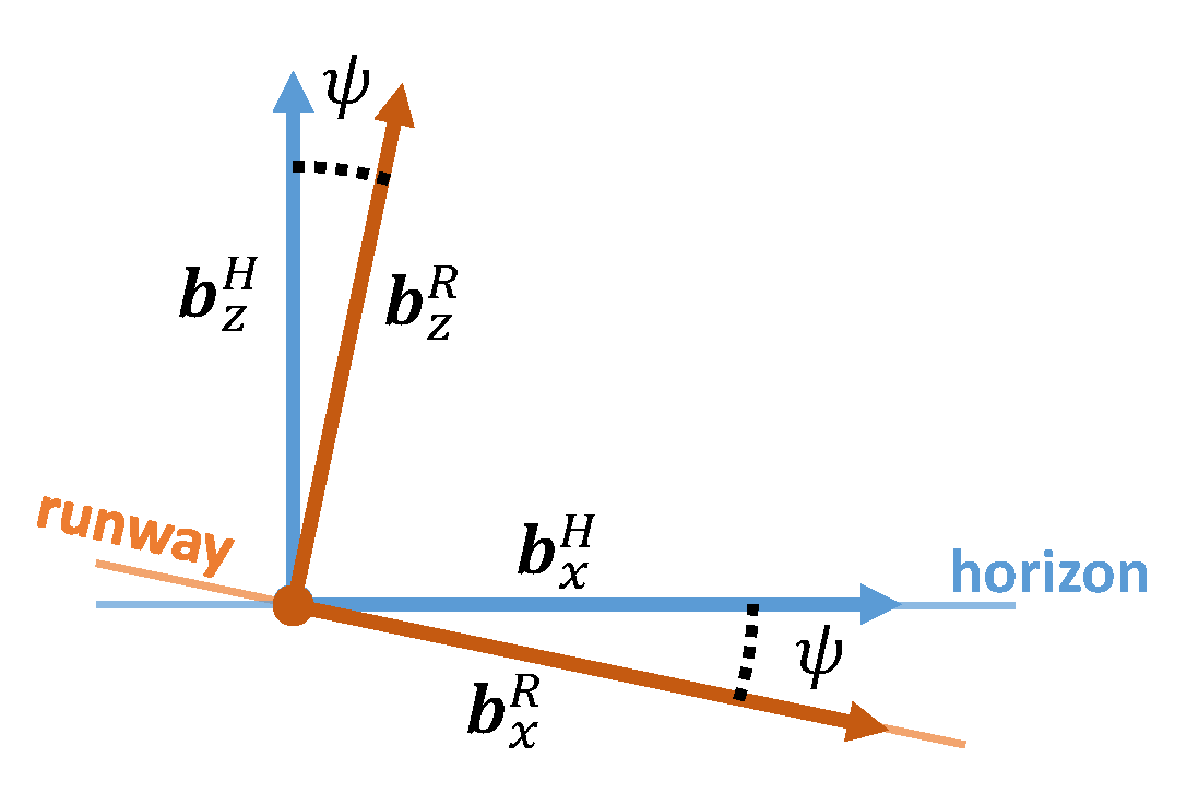
In consideration of a possible slope of the runway with respect to the horizon, three two-dimensional reference frames are introduced, for conveniently writing the equations of motion and measuring the take-off distance. The horizon frame (
) is centered in the initial aircraft standstill point, and features the first axis (
) along the horizon (normal to gravity), and the second one (
) aligned with gravity and pointing upwards. The runway frame (
) is again centered in the standstill point, with the first axis (
) along the runway and pointing towards the take-off direction, and the second axis (
) normal to the runway surface, pointing upward. The two frames are, therefore, made different by a non-null rotation of an angle
, measuring the slope angle of the runway with respect to the horizontal, as in
Figure 2.
The take-off distance, intended as the primary measure of performance of the aircraft in the take-off maneuver, is defined along the first axis of the runway frame, .
The third reference frame adopted in the description is the body frame (), which is attached to the aircraft, centered in the center of gravity (), with the first axis () defined as the roll axis, and the third one () defined as the yawing axis.
Similar to the aircraft in flight, pitch angle is defined between the longitudinal axis and the horizon (i.e., and ). Due to the specific design of the undercarriage, to an arbitrary choice of the roll axis of the aircraft, as well as the presence of a non-null runway slope , in standstill (initial) condition the pitch angle may be a non-null value . The time derivative of pitch, namely pitch rate, is defined as .
The position of
in the horizon frame can be described by coordinates
and
, whereas in the runway frame by
and
. Similarly, the intensity of the velocity vector can be defined as either
In this analysis, no wind speed relative to the ground has been considered (still air hypothesis), yielding a perfect equivalence of the velocity and airspeed vectors.
Climb angle
is defined between the velocity vector and the horizon (
), and may be analytically described through the scalar components of the velocity vector of
, respectively,
and
, as
Concerning the geometry of the aircraft, the thrust line has been considered potentially misaligned with respect to the roll axis by an angle , and displaced with respect to along the axis by a value . The value of the absolute (i.e., always positive) distances between and the main and nose wheels can be defined as and along the body axis .
2.2. Dynamic Equilibrium in Take-Off
2.2.1. Ground Run Phase
Considering the ground run, this can be analytically defined as a condition where both reaction forces on the main and nose wheels are non-null. In this condition, pitch rate
, and climb angle
. Written in scalar components in the runway reference, momentum balance and angular momentum balance yield, respectively, the first two and the third equations in the following system
where
m is the mass and
is the barycentric moment of inertia about the pitch axis,
W is aircraft weight force. Quantities
L,
D,
represent the aerodynamic lift and drag force components, and the barycentric pitching moment. Force
represents thrust, and
its moment about
. The reaction forces of the main and nose wheels are lumped in the momentum balance equations, bearing the term
as a reaction force normal to the ground, and
tangential to the ground, where
is a friction coefficient. Conversely, in the angular momentum balance equation the moment of the reaction forces is represented by
. Finally,
is the angle of attack, and represents the misalignment between
and
in this context.
In analytical terms, the components just introduced and appearing in balance equations (Equation (
3)) are defined as follows,
where the reaction normal to the runway on the nose and main wheel are, respectively,
and
,
g is gravity,
the density of air,
S the area of the wing planform and
c the mean aerodynamic chord of the wing. Parameters
,
, and
are the lift, drag, and pitching moment (barycentric) coefficients pertaining to the aircraft in ground run. These are obtained from the specific angle of attack
attained during the ground run, itself a result of the incidences of the aerodynamic surfaces with respect to the fuselage, and of the misalignment between
and the ground direction
. They are also functions of the deflection of the controls
of the elevator and
of the canard (if available, as on a three-surface aircraft), which both assume increasing values in the model whenever deflected downwards. Furthermore, it should be remarked for practical purposes that the values of these coefficients pertain to a take-off configuration, i.e., typically with slats and flaps deployed, and not to a clean one, typically adopted for computations in cruise.
From Equations (
3) and (
4), it is possible to obtain expressions for the total, main wheel and nose wheel reaction forces, yielding
The forces and moments acting on the aircraft according to the model just introduced are graphically summarized in the sketch presented in
Figure 3.
Here, each action is portrayed as assumed positive in the model.
2.2.2. Rotation Phase
The rotation phase is triggered upon reaching a null value of the reaction force on one of the wheels, typically the nose wheel, so that
The latter can be substituted in Equations (
4) and (
5), yielding simplifications in the definitions of
and
.
The nullification of the reaction force on the nose wheel is accompanied by a rotation of the aircraft in the vertical plane, measured by a non-null pitch rate q. Considering a negligible motion of the normal to ground, i.e., a null , the value of shall be null by hypothesis, thus resulting in the equivalence .
The equations of motion are formally the same as in Equation (
3), with the only exception of the angular momentum balance (third equation) which does not equate to zero, since a rotational acceleration
may be non-null in this phase.
2.2.3. Airborne Phase
The aircraft is airborne when all ground reaction forces reach zero. In accordance with usual flight dynamics performance analyses, the equations of motion in this phase can be conveniently written in the horizon frame, yielding in scalar components
Clearly, in this phase the aircraft is free to climb, and
in general, where
.
2.2.4. Evaluation of the Take-Off Distance
The take-off distance, since it is bound to a minimum clearance with respect to the ground, needs to be computed as the projection of the entire take-off trajectory on the
axis in the runway frame. Considering the ground run and rotation phases, the first scalar component in Equation (
3) can be integrated yielding the corresponding
distance value directly. For the airborne phase, the corresponding contribution along
can be computed applying the rotation
fed with the result of the integration of Equation (
7), and taking the first line of the result.
Thanks to Equation (
8), it is possible to represent the position and orientation of an aircraft in take-off through an array composed of three scalars only, as
The corresponding state array of the system is—as usual for a mechanical system—composed of
and its time derivative
, so that
Similarly, an array of controls can be defined as
, which in general will be
Clearly, for a two-surface aircraft the second scalar control in Equation (
11) can be taken out of the formulation.
Based on the state and control arrays just introduced, the value of the take-off distance
can be computed from the integral
As anticipated, the take-off maneuver is over upon reaching a certain clearance from the runway level, hereby defined as
, and defined in the direction of
. The final time
appearing in Equation (
12) corresponds to a condition when the aircraft has reached the threshold clearance, or analytically
.
2.3. Aerodynamics Modeling
The equations of motion Equations (
3) and (
7), with definitions in (
4) and (
6) invariably hold for virtually any aircraft which can be modeled from a lateral view with two components in the undercarriage, namely a main and a nose wheel. The difference between a two-surface and a less conventional three-surface configuration impacts the model through the definition of the aerodynamic coefficients.
Considering both configurations, the following structure is adopted in this research for the lift, drag, and barycentric pitching moment
In Equation (
13) the derivative of
and
represent sensitivities with respect to the angle of attack
,
, and
those with respect to the deflection of the tail elevator
,
, and
those with respect to the deflection of the canard control surface
. The sensitivities
and
represent stability derivatives with respect to the pitch rate
q. Coefficients
,
,
k, and
do not depend on any variable.
All coefficients are, in principle, functions not only of the general arrangement of aerodynamics surfaces (two-surface vs. three-surface), but also of the features of the take-off configuration. In particular, with respect to typical clean aerodynamic configuration (e.g., in cruise), in take-off an aircraft shall feature extracted landing gear, and a non-negligible wing flap/slat deflection. However, for modeling purposes, it is common practice [
22,
23] to have the effect of a change in the configuration with respect to the clean one act through a separated additional effect independent of kinematics (i.e.,
,
q) or elevator/canard control (
,
), yielding:
where superscript
stands for clean configuration, whereas
and
mark the flap and landing gear contributions.
Values of the aerodynamic coefficients in Equations (
13) and (
14) can be obtained as functions of the aerodynamic properties of the wing, tail, canard, flap/slat system, and landing gear. These relationships can be obtained through semi-empirical models as typical in a design phase (specifically, standard estimation procedures by Roskam [
22] and Pamadi [
23] have been adopted in the present research, where aerodynamic coefficients are computed based on statistical regressions, for a basic geometrical sizing and assigned two-dimensional aerodynamic properties), from virtual (i.e., numerical) experiments, or from experiments typically in the wind tunnel.
The contributions to an aerodynamic coefficient by a given aircraft component on the aircraft (e.g., contributions to
by the wing, or by the tail) are then suitably merged, to bear a global value pertaining to the aircraft as a whole, as required to populated the model in Equations (
13) and (
14) (see again the procedures proposed in [
22,
23]). Considering the contributions of the wing and tail, the classical two-surface modeling adopted for flight dynamics computations can be adopted [
23]. For a three-surface aircraft, a corresponding complete formulation has been developed and thoroughly shown in [
9].
It should be remarked that the aerodynamic coefficients in the model represented by Equations (
13) and (
14) are considered constant assigned parameters in the present research. In other words, once the configuration, including flap/slat deflection, is assigned, the values of all aerodynamic coefficients are known and constant for the duration of the take-off maneuver. Furthermore, considering transient effects, like the reduction in ground effect when increasing the altitude, working with constant coefficients equates to considering an average behavior of the aircraft during the maneuver. Where, on the one hand, this is a simplification, the comparisons carried out in this work, especially among two-surface and three-surface aircraft, are carried out invariably adopting the same hypothesis, and are, therefore, fair.
Thrust Modeling
Since take-off is a maneuver associated with a significant change in velocity (and, consequently, in airspeed), it is important to account for the effect of a change in airspeed on the performance of the propulsion system. This is particularly true for propeller-driven aircraft, since thrust is usually decreasing with speed in take-off, and failing to account for that may produce an over-estimation of the take-off performance (i.e., an erroneously low take-off distance). At the level of detail of the flight mechanics model considered in this text, it is possible to include a simple first-principle model to account for this variability, based on the assumption that the propulsive power available from the engine and propeller is constant with airspeed. As a result of that assumption, the available thrust
T can be written as
where
is the shaft power of the engine, and
is the efficiency of the propeller, itself a function of the advance ratio
. In this work,
is considered independent of the wind speed, assumption clearly acceptable if the sole take-off is considered.
Take-off is usually carried out at a constant throttle setting, hence the latter is not considered as a control parameter.
3. Optimal Take-Off Performance
As stated in the introduction, the present research is focused on seeking the optimal take-off performance attainable with a two-surface and a three-surface aircraft. By assessing the corresponding measurements of performance, the improvement provided by a configuration with respect to the other will be demonstrated. However, in order to produce a fair and practically meaningful performance analysis, the optimal performance needs to be studied accounting for a physically achievable take-off maneuver.
The meaning of this requirement is two-fold. Firstly, the maneuver should take into account the need to control the aircraft in the longitudinal plane via a single stick control, even when considering a three-surface aircraft. In other words, even though the canard control surface introduces a new independent control in the longitudinal plane (in fact, a redundant control), both controls on the longitudinal plane (i.e., both the elevator and canard deflections) need to be linked to the same stick control. This implies that no time phase between the actuation of the two controls can be envisaged, or in other words, that the canard and tail need to move simultaneously. On the other hand, the relationship between the motion of the two deflections on a three-surface aircraft, i.e., the elevator and canard respective response to a motion of the stick, is not hypothesized a priori, and will be instead an outcome of the present analysis. Secondly, the motion of the aircraft during the take-off maneuver is constrained by obvious clearance and, more generally, kinematic limitations, so as to avoid for instance contacts of the fuselage with the runway (e.g., tail strike issues), or excessive rotation rates. This type of limitation can be naturally applied in an optimal performance analysis, by means of properly-defined mathematical constraints.
In the next sub-section, the framework adopted for the optimal analysis of take-off performance will be described in detail.
3.1. Measure of Performance and Structure of Control
The selected measure of performance for take-off is
, as defined in Equation (
12), which is, therefore, promoted to objective function in the optimization. The reason has been stated in the introduction, and is primarily bound to the general good correlation of this parameter with a reduced noise and chemical footprint on ground. It is also an interesting flight performance parameter in its own respect.
It is apparent from Equation (
12) that the take-off distance is a function of the control action
, in principle a continuous function of time.
A quasi-steady approach has been adopted for aerodynamics, wherein aerodynamic coefficients are updated based on the instantaneous current condition of the aircraft.
In a numerical framework, considering a piece-wise constant representation of the control action over the take-off maneuver on a velocity grid of arbitrary resolution and composed of
N nodes, it is possible to assign the control action analytically by defining an array of control velocities and a corresponding set of control values, so that
where
is the numerical representation of
.
For a two-surface aircraft, clearly
is simply taken out of the formulation. Thinking to the more complicated three-surface case, on account of the considerations just introduced (see the preliminary part of
Section 3), a change in one of the controls should imply a simultaneous change in the other (time co-location effect). This is not a priori guaranteed by the numerical representation in Equation (
16), where for each node the values of
and
should be related according to a bound modeling the mechanical link between the two. However, before imposing such a link, we make at this level a further hypothesis, which simplifies the problem while further increasing its practical meaning. Actually, considering that during a take-off maneuver, the manually operated aircraft stick is actuated typically only once and only a certain amount—usually, the control column is pulled gently by a certain amount—the representation in Equation (
16) is reduced to the following two-nodes one
where a null value
has been further hypothesized, representing null velocity at the beginning of the take-off run. The representation in Equation (
17) assumes that the control action in the take-off run can be described by a set of five parameters for a three-surface aircraft, namely the initial deflections
and
, which are the values of the controls kept constant from a standstill condition up to a velocity
, and a second couple of deflections
and
, obtained step-wise action on the control column at time
. Clearly, for a two-surface aircraft, the representation in Equation (
17) is even simpler, since
is taken out of the formulation, and consequently the set of parameters to be assigned is reduced to three, namely
,
, and
.
It can be pointed out that for a three-surface aircraft the simplification of the control representation hypothesized passing from Equation (
16) to (
17) offers a significant simplification in the design of a mechanical link between the elevator, the canard, and the motion of the control stick. Actually, for whatever choice of the four scalar parameters defining the couples
and
, it is possible to obtain a corresponding linear relationship as
which interpolates both conditions. This allows one to design a physically linear kinematic link between both surfaces and the yoke, greatly simplifying the kinematic connections and general arrangement of the control line. The same would not be guaranteed a priori when adopting a representation based on a number of nodes grater than two.
Based on the representation introduced in Equation (
17), it is possible to set up an optimal problem where
is expressed as a function of
instead of a generic
.
3.2. Free End-Time Problem and Definition of the Set of Optimization Parameters
For an assigned control, the evaluation of
is bound to the knowledge of
, the final time of the take-off maneuver, corresponding to the following recursive definition
It is possible to configure the optimal problem as a free end-time one. This can be treated considering
as an additional optimization parameter, such that time
t is expressed as
with
defined as an arbitrary reference time value. The objective function can be correspondingly computed as
In Equation (
21), quantities
and
are obtained by recurring to the mathematical definition of the time derivatives with respect to a scaled time, which according to Equation (
20) yields for a generic function
Therefore, for the derivatives of the state array it is readily obtained that
wherein the scalar
required for evaluating Equation (
21) can be extracted.
In order to close the free end-time problem, Equation (
19) is promoted to an additional constraint in the optimization.
To conclude, adopting the representation of the control time function in Equation (
17) and defining the problem as a free end-time one, the set of optimization parameters to be considered for a two-surface aircraft can be defined as
whereas for a three-surface aircraft
Both sets are used to minimize for the respective aircraft architecture the take-off distance, invariably defined as
according to the same constraint on final time
From a numerical stand-point, the latter Equation (
27) is managed by means of a couple of inequality constraints. In analytical terms, it is imposed that
where
and
are chosen suitably close to
. This eases convergence for the numerical optimization method, at the price of a possible small inaccuracy on the final distance from ground to be reached.
3.2.1. Physical Constraints
As previously stated, a set of physical constraints need to be added to produce a physically feasible take-off maneuver. In addition to the constraint in Equations (
27) and (
28), four more physical constraints are considered.
Stall prevention. The practical means by which stall avoidance is pursued are two-fold. Firstly, the value of the lift coefficient is forced not to become too close to the maximum attainable, in order to avoid reaching the stall condition for instance in presence of a disturbance in the angle of attack. Secondly, a safety speed of 120% of the stall value needs to be attained at the end of the take-off maneuver, as per standard regulations for certification. In analytic terms, these constraints read:
A safety margin of 95% has been considered in the computations to follow. Notably, where a stall value for the entire aircraft can be computed based on the models adopted, separate stall on each surface has not been considered explicitly in computations. Instead, surfaces were checked a posteriori for stall in sample cases, to avoid considering non-physical maneuvers. Due to the relatively mild motion of the control surfaces, and the generally slow maneuvers, no issue was ever found in this sense, at least in the scope of the present analysis.
Pitch rate and climb angle. These quantities are limited so as to avoid excessive load factors (pitch rate), as well as an excessively steep climb at the end of the take-off maneuver, which is unusual in practice. In analytic terms,
Tail strike prevention. In order to avoid the tail hitting the ground in the rotation phase (tail strike), it is possible to include a constraint on the clearance of the potential point of contact of the tail cone, in a direction normal to the ground surface. In analytic terms, when defining
the potential point of contact of the tail cone in a rotation around the point of contact of the main wheel with the ground, the coordinate
shall measure its position in the runway reference. Despite the aircraft is not rotating around this point in the rotation phase, this is an acceptable approximation for the level of detail of the model considered in this research. Therefore, a constraint can be written as
where
represents a minimum threshold for the clearance.
Bounds for control sequence coherence. Recall from Equation (
17) that the control input is described through a sequence of values of
and
which are enforced upon reaching a certain speed, as in real field practice. In order to avoid an unrealistic setting by the optimizer, the speed
is bound between zero and the take-off speed. Similarly, for the elevator in a two-surface configuration,
needs to be more intensely negative than
, in accordance to practice (i.e., pulling on the yoke during take-off, to trigger rotation). In analytic terms, this yields the following two bounds for optimization variables
To explain this point better, it should be remarked that the constraint highlighted in Equation (
32) has been included to stop a time-marching simulation in case the set control pull-up airspeed
is not reached before actual lift-off. The idea behind it is that a control pull-up (whatever its intensity within the prescribed bounds) would not significantly alter the resulting take-off distance if imposed after liftoff. Furthermore, a take-off maneuver requiring the pilot to change the control setting during or soon after liftoff would be practically too difficult to implement, due to a possibly excessive workload in the phase following liftoff. This would produce results with an academic validity, but with hardly interesting in practice. Concerning the second inequality in Equation (
32) a push on the controls is not a realistic control strategy for obtaining a liftoff. Therefore, such regulation approach was taken away a priori from the space of solutions.
The overall numerical scheme highlighted in this section is based on the computation of the take-off distance . The latter can be carried out in practice via an adaptive Runge-Kutta integration method.
4. Application to a General Aviation Aircraft
As stated in the introduction, a comparative analysis between the performance of a conventional two-surface aircraft and one with three-surface is of interest, to better understand whether the latter might produce an increase in take-off performance. This would come besides the increase in cruise performance already demonstrated in [
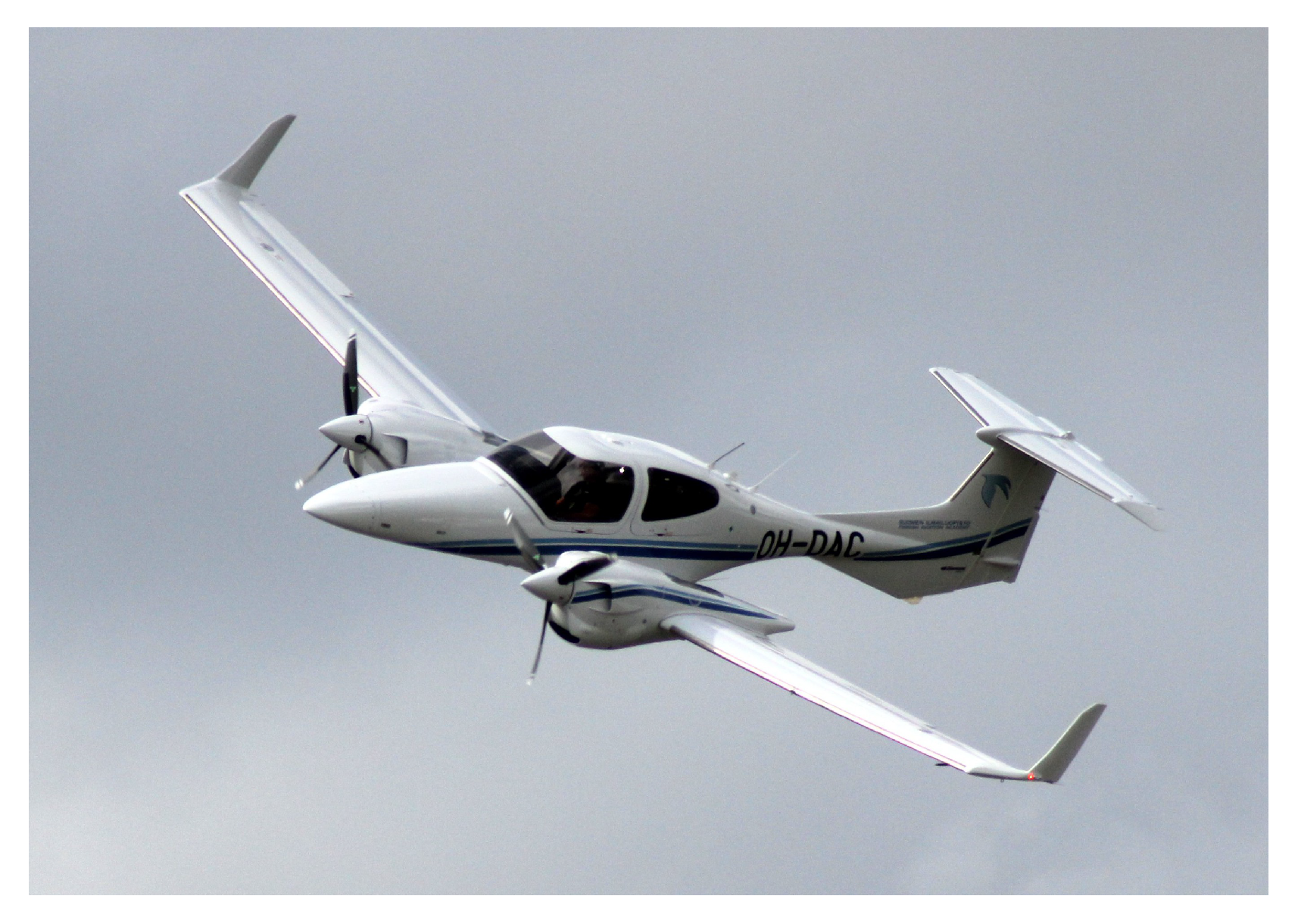
9]. In order to set up a fair comparison, a thorough performance assessment of a two-surface aircraft will be shown first on the data of a Diamond DA-42 [
24], a light twin-propeller aircraft certified in CS-23 normal category. Not only will the global performance optimum be investigated, but also the general behavior of the merit function, i.e.,
, to better understand the quality of the optimal solution and the behavior of the performance and constraints. Next, the performance of an equivalent three-surface aircraft will be evaluated, obtained guaranteeing the same static margin and overall control volume of the baseline two-surface version [
9]. The details of the analysis will be shown in the respective subsections to follow.
4.1. Optimal Take-Off of Two-Surface Aircraft
The basic data of the DA-42 (see
Figure 4) are reported in
Table 1. In order to explore the
performance, a range of values for
,
and
are considered. Furthermore, a set of constraining values are adopted to study the effect of all constraints defined in
Section 3.2.1. These are shown in
Table 2.
4.1.1. Parametric Analysis
Based on the modeling introduced above, the take-off distance
for a two-surface aircraft can be computed once the values of
,
, and
are assigned. A representation via contour plots of the result, as a function of two quantities and for an assigned value of a third parameter, is shown in
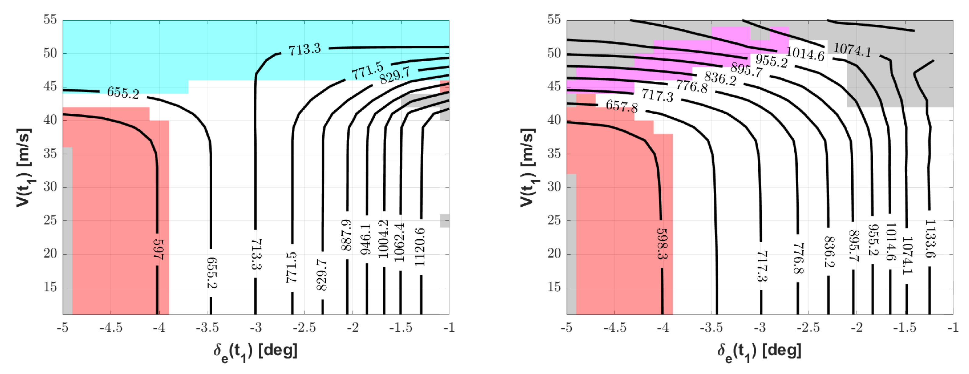
Figure 5 and
Figure 6. Respectively, in the former the assigned parameter is the pull-up speed
, whereas in the latter the value of the initial deflection
. In practice, these two parameters are
the speed for which the pilot imposes a change in the deflection of the elevator, and
the initial value of the elevator deflection kept by the pilot from the start of the take-off run until reaching
, according to the adopted model.
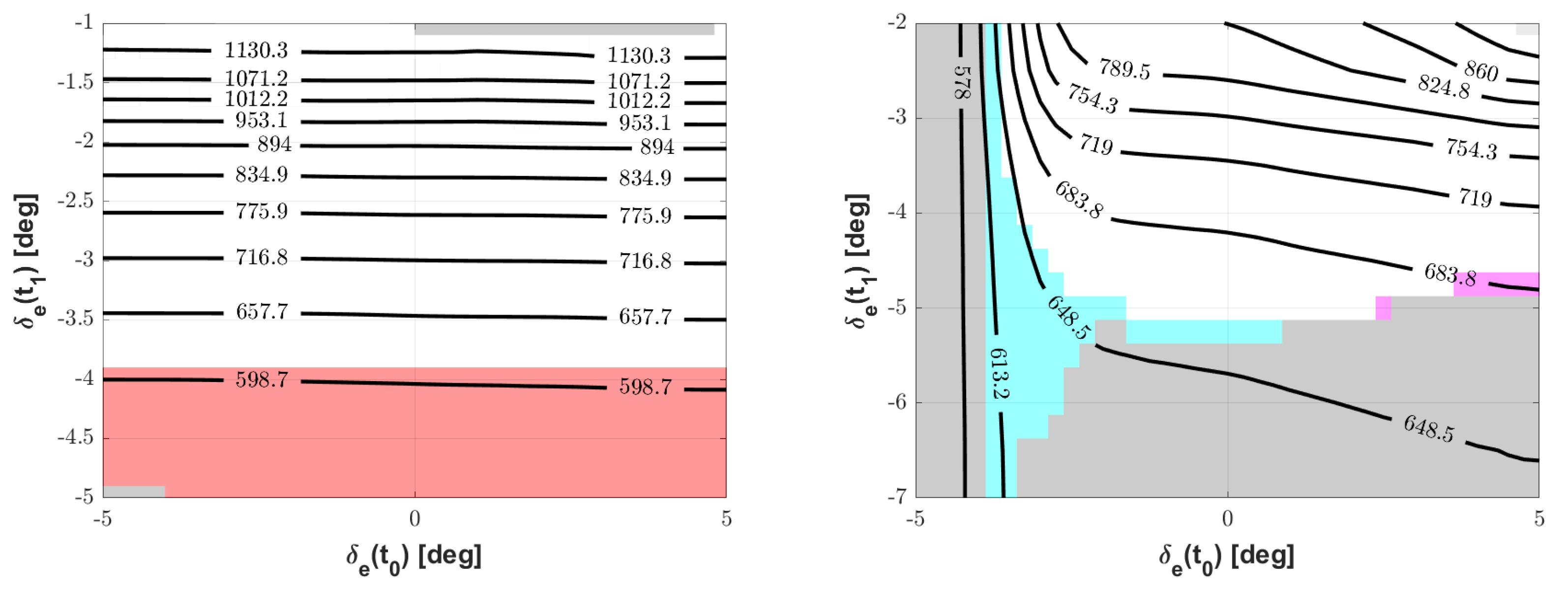
Considering the plots in
Figure 5, for a lower control pull-up speed (left) the effect of the initial control setting
is almost null. For increasing the absolute values of the final
, a decreasing (i.e., improving) value of
is obtained. However, the red area to the bottom of the plot is where the tail strike constraint is hit, thus limiting a further decrease in
.
For a higher control pull-up speed (right plot), the effect of the initial elevator deflection is more marked, showing for a higher value generally higher results (to the right of the plot), culminating in the activation of the maximum pitch rate constraint (purple area) for more intense target deflections after the control pull-up. This corresponds to physical conditions where the initial part of the take-off run is operated pushing (instead of pulling as typical) on the control, with the effect of a tendency to keep the aircraft below , resulting in a longer . In other words, take-off is sought through an increase in speed, rather than an increase in the angle of attack, bearing a longer distance.
Conversely, for lower values of
(left area of the plot), corresponding to a condition where the control is more intensely pulled towards the final target value since the beginning of the take-off run, lower values of
might be achieved. However, the cyan area is associated to a condition where the final speed of the maneuver, i.e., when
is reached, is lower than
, so that the take-off maneuver is complete without even pulling the control at some point. This violates the constraint in Equation (
32). For completeness, the grey areas in
Figure 5 correspond to a simultaneous violation of two or more of the considered constraints.
Looking at the contour lines in both plots of
Figure 6, two macro-regions can be spotted, corresponding to lower or higher values of
. For lower values of
, the effect of the latter is rather limited, whereas a significant effect is obtained from a change in
. For both plots—i.e., for both considered initial values of
—a low
is obtained on the border of the tail-strike constraint violation area (bottom left corner on the plot).
For higher values of , a significant gradient with respect to the latter is observed. For a higher value of (right plot), is increased in this area as a result of a prolonged pitch-down command on the elevator, which retards the take-off maneuver, producing higher take-off distances. Moreover, for excessively high control pull-up speeds, a change in elevator deflection produces an excessive pitch rate, represented by the purple strip towards the top of the plot.
On the other hand, for a low, negative
(left plot), it should be noted that the values to the left and to the right of the
−3 deg value on the horizontal axis correspond to the two sides of a limit condition, where pitch control keeps the same value all along the take-off maneuver. To the left of this line, for higher values of
(top-left part of the plot), the solution in terms of
remains stable, but the cyan constraint violation area indicates that the maneuver ends (i.e., final altitude is reached) before any action on the controls. This is similar to the scenario encountered on the right plot in
Figure 5. Conversely, to the right of the line, a solution where a pull-down action on the elevator control is carried out is actually considered. This is obviously associated to a ramp-up in the
performance, which is of little practical relevance.
The plots in
Figure 5 and
Figure 6, besides introducing a good deal of information, provide examples of the rather articulated outcome of the performance analysis. They also provide elements for interpreting and forecasting the position of the global optimal solution.
4.1.2. Optimization
The optimal solution for a two-surface aircraft is obtained by minimizing the
function in Equation (
26), subject to constraints in Equations (
28)–(
31), with optimization parameters
defined in Equation (
24), bounded as per Equation (
32).
As shown in the partial analyses of the functional
proposed in the previous paragraph, the gradient of the merit function with respect to the selected optimization parameters appears smooth, which makes the problem treatable by means of a gradient-based approach. The result of the optimization is presented in
Table 3.
The behavior of the optimal control input is in line with the preliminary analyses proposed in the previous paragraph, and also with practice. A significantly negative initial deflection , is required followed by a control pull-up action, which produces a more intensely negative .
A three-dimensional close-up view of the
function in the vicinity of the optimum, displayed in
Figure 7, shows that the latter is actually constrained by two constraints, namely tail strike avoidance and the upper bound on the airspeed for the pull-up maneuver (
). From the same plot, it can be perceived that near-optimal solutions and broader spans of usable control pull-up speed
can be obtained with a somewhat less intense target elevator control
.
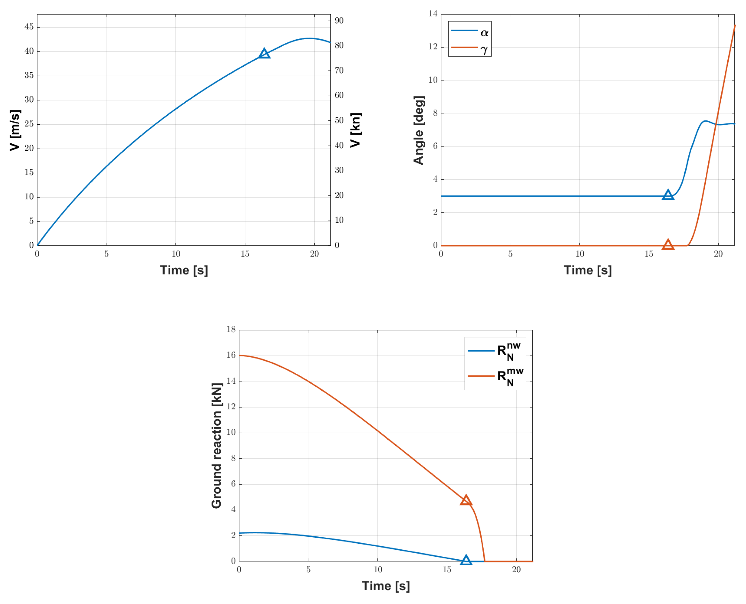
The optimal result in terms of time histories of airspeed, angle of attack, climb angle, and ground reactions on the front and main wheels for the optimal solution is shown in
Figure 8.
The latter shows a rather regular maneuver in accordance with practice and experience.
4.2. Optimal Take-Off of Three-Surface Aircraft with Redundant Longitudinal Control
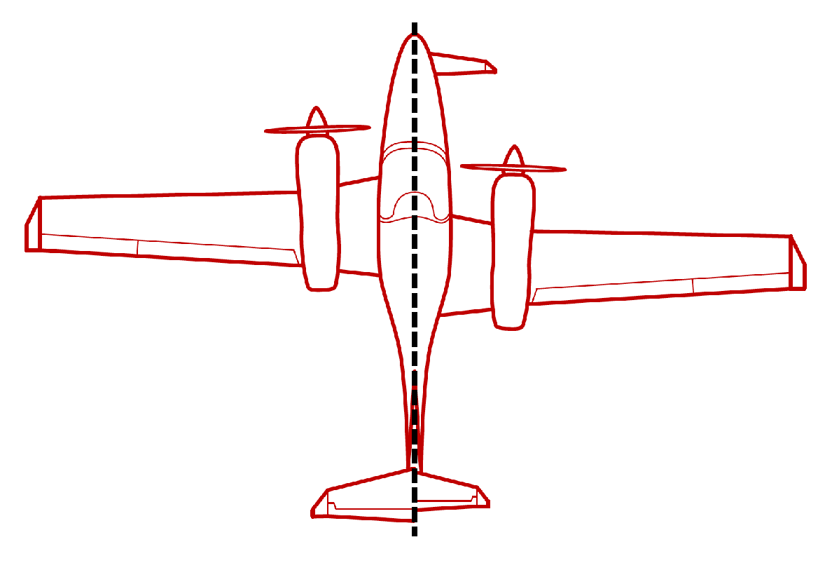
In order to provide an as fair as possible comparison to the two-surface aircraft, thus showing the effect of just having a three-surface configuration instead of a standard two-surface, a new aircraft has been obtained from the baseline DA-42, adding a canard (see
Figure 9 for a comparison). The sizing of the new three-surface aircraft has been carried out based on two considerations. Firstly, to keep the airborne stability and control performance similar to that of the reference DA-42, the static margin and the overall control volume have been preserved, as described in detail in [
9]. Correspondingly, the wing has been relocated backwards with respect to the baseline. Secondly, the landing gear of the new aircraft has been shifted backwards, in order to keep the same distance between the center of gravity and the main landing gear as on the original DA-42. Concerning the tail clearance for the activation of the tail-strike constraint, this has been set in order to preserve the same maximum pitch angle of the DA-42 on ground. Basic data for the three-surface configuration are recalled in
Table 4.
The optimal problem solved for the three-surface aircraft is the same considered for the original DA-42, with the only difference due to the set of parameters, which is that reported in Equation (
25) instead of Equation (
24). Clearly, the larger number of parameters makes the graphical exploration of the cost function
very impractical.
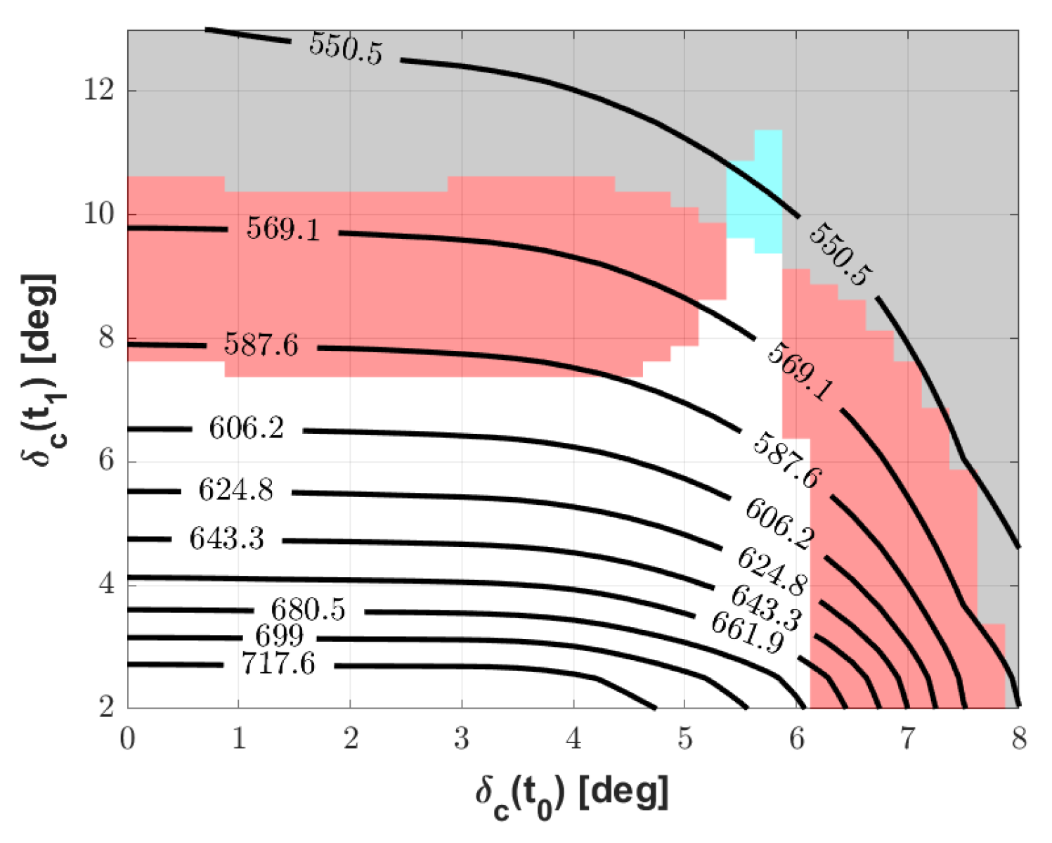
4.2.1. Example of Parameter Analysis of the Merit Function
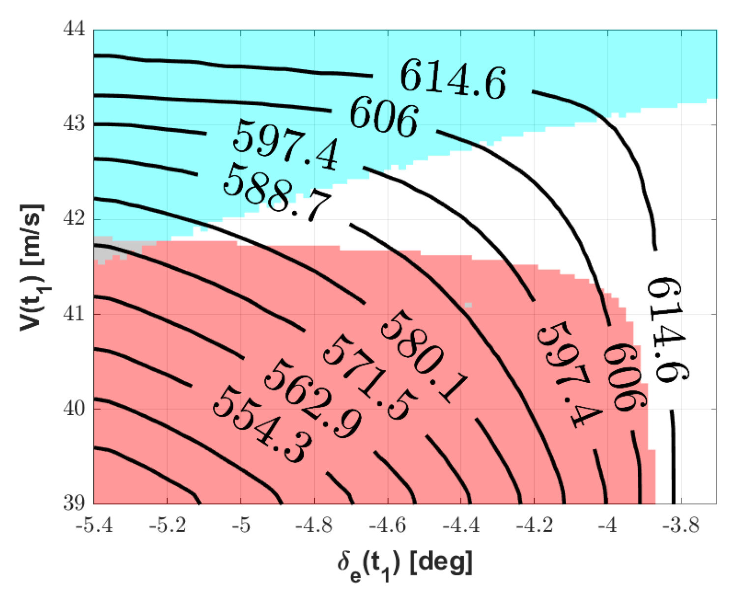
As an example of the trend analysis on the optimal solution when dealing with a three-surface aircraft,
Figure 10 displays the behavior of
for an assigned and constant position of the elevator, i.e.,
−2 deg, and a given control pull-up speed
41 m/s. Therefore, the take-off distance is expressed as a function of the canard setting before and after an action on the control, respectively,
and
. It can be observed that for a sufficiently high final deflection
of the canard a significant reduction in
can be achieved. As previously pointed out, the profile aerodynamics corresponding to this condition have been verified a posteriori, showing that it does not entail a stall of the canard. However, the tail-strike constraint is hit for a broad set of lower initial values of
(red area). Similarly, for high initial values of
, to the right of the plot, the tail strike constraint is again activated, irrespective of the final value of the canard deflection. Optimal values of
can be found in the top-right region of the plot (see the contour lines), in a pocket surrounded by conditions where either tail-strike or late control pull-up maneuver are activated.
Unfortunately, due to the dependence of the merit function on more parameters,
Figure 10 does not allow to draw general conclusions. However, from a mathematical standpoint, a good regularity of the cost function and of the constraints allows to deploy a gradient-based method to investigate the actual optimum.
4.2.2. Optimal Solution
In case an optimization is carried out based on the five optimization parameters in Equation (
25), a solution featuring a roughly constant value of the canard deflection is obtained (similar to what can be seen in
Figure 10). The quantitative solution is presented in
Table 5. This is interesting, since it shows that the use of the canard like a flap instead of a continuously deflectable surface like a tail elevator, may be envisaged. Instead, a mild negative deflection of the elevator is required, as expected.
The optimal solution for the original DA-42 baseline can be retrieved for comparison in
Table 3. It can be observed that a non-negligible 7% reduction in the optimal take-off distance
is obtained by moving to a three-surface configuration.
4.2.3. Considerations on Control Linkage
The optimal values of canard and elevator deflection in
Table 5 for the three-surface aircraft have been investigated considering the five optimization variables, and, in particular, the initial and final values of the elevator and canard deflection, as independent quantities. However, as explained in paragraph
Section 3.1, the modeling adopted for this study allows to effortlessly envisage a linear relationship between the deflections of the elevator and canard, which would be easy to design and manufacture in the field. The ensuing linkage would constrain both control surfaces to move as a result of a deflection of the control yoke, making the mathematical solution obtained from optimal analysis practically achievable.
Considering Equation (
18), the values of
−0.169 and
0.225 rad for the optimal solution in
Table 5.
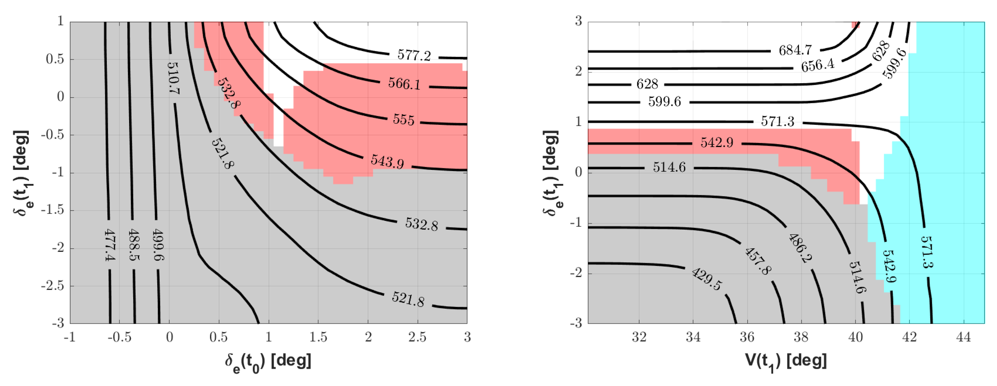
A first consideration concerning this result is on its robustness. By performing an analysis of the cost function distance
in the vicinity of the optimal solution, it can be observed that the latter is—as expected—significantly constrained. This is shown in
Figure 11, where on the left plot the values of
and
are presented on the axes, and
has been set at its optimal value, and on the right the
and
are free parameters, and
has been set at the optimal value (clearly,
is set according to the linkage law, and its initial and final values are correspondingly not free parameters any more).
This suggests that the choice of this linkage might introduce a certain sensitivity from the actual choice of parameters in a take-off maneuver. In other words, if not deflecting the yoke of the right amount or at the right control pull-up speed, the resulting take-off might easily produce the violation of a constraint, which, physically speaking, might for instance produce a tail-strike.
This suggests, for practical purposes, choosing a slightly sub-optimal condition, i.e., a somewhat higher and the corresponding set of five parameters. If on the one hand this would not ensure the feasibility of the globally optimal take-off maneuver, it would increase on the other the robustness of the solution, increasing the practical safety of the actual maneuver, mathematically represented in particular by a less critical compliance with respect to tail-strike and maximum pitch-rate constraints.
A second consideration stems from the results of the optimization of the linkage for cruise, proposed in [
9]. The corresponding values of the coefficients in Equation (
18) is
0.461 and
0.329 deg, which are significantly different from those obtained in the present study. When applied, the values just mentioned produce the optimal achievable condition reported in
Table 6, which, in particular, correspond to a
significantly above the optimal value shown in
Table 5, and coincidentally closer to the value achievable with a two-surface aircraft (see
Table 3).
This is not surprising, since the requirements which the synthesis of the cruise linkage have been based upon do not correspond with those driving the analysis presented in this paper. However, this shows that capturing both optimal working conditions in cruise and take-off with a single linear linkage is not generally possible. An ensuing suggestion which may be obtained is that, for a practical implementation of a control on a three-surface aircraft, a linear mechanical control linkage may be adopted with a tuning wheel in it, capable of altering the linear linkage for different phases of the flight. Of course, a conceptually easier way to develop such a control would be that of departing from a direct mechanical linkage, implementing an electronics-augmented system instead. In the latter scenario, a change in the linkage characteristics would be obtained by simply programming (i.e., scheduling) the coefficients of the linear link as a function of the flight phase. This may be identified by an action of the pilot, switching to either a terminal phase or cruising mode.
5. Conclusions
In the present research, the increase in the take-off performance of a three-surface aircraft with respect to a two-surface one was investigated.
Despite a good deal of literature that exists regarding the topic of aerodynamics and aeroelasticity of canard and three-surfaces configurations, the specific behavior in terminal maneuvers of such aircraft is not currently covered.
Furthermore, as opposed to the existing literature concerning take-off optimization, typically focused on providing means of improving take-off key indicators (e.g., loads, ground clearance, rolling distance and noise), this research tries to assess the advantage of an assigned (i.e., non-negotiable) three-surface configuration, shown to be capable of successfully reduce trim drag in cruise in prior research, also in a take-off maneuver.
An original description of take-off has been proposed starting from a classical lumped-coefficient approach. This is typical to flight mechanics, and allows to seamlessly cover both two-surface and three-surface aircraft. After introducing a model for take-off dynamics, the take-off maneuver was modeled as a reaction to a prescribed time history of controls. The latter has been envisaged taking into account three desired features:
Simplicity of the time history, so as to allow a pilot to carry out the maneuver;
A minimal set of descriptive parameters, in order to reduce computational cost in an optimal analysis;
A set of parameters compatible with the need to manufacture a linear linkage connecting the elevator and canard surfaces.
An optimal analysis of the take-off performance was carried out at first on a baseline two-surface aircraft. For this case, a visual study of the cost function, identified in the take-off distance , was possible, thanks to the very reduced number of optimization parameters.
Next, a qualitatively similar optimal analysis was carried out on a three-surface aircraft, obtained from the baseline in a way such to make the two equivalent in a stability and control authority sense, both in flight and in take-off.
The simulation model, as well as the implementation of some constraints in the optimization have allowed obtaining a streamlined algorithm, computationally manageable without difficulty and imposing irrelevant machine time overheads on standard commercial computers. This, in turn, makes the envisaged procedure a good asset in a preliminary design or performance verification phase.
The result of the optimal analysis on the three-surface aircraft has shown a 7% increment in performance achievable by suitably making use of redundant control on the pitch axis. No stall issues on the control surfaces have been encountered in the performance analysis phase, thanks to the generally mild deflections required for maneuvering. The optimal region is generally constrained by tail-strike or an excessively delayed pull-up, so that liftoff takes place before an actual pull on the control yoke.
Interestingly, the optimal result in this configuration features a roughly constant value of the canard deflection during the maneuver, suggesting its use as a flap more than of a control surface. A potential weak robustness of the optimal solution was found, meaning that the achievement of the global optimum would come only for a precise take-off maneuver, and with the risk of incurring in physical limitations (such as tail-strike) in case of small deviation from it. This suggests to consistently drift in practice towards a sub-optimal maneuver, granting a reduced advantage on take-off distance, with the plus of a lower risk of accidents in case the pilot’s action on the controls were not perfect.
Finally, from the comparison of a possible structure of a linear linkage between the canard and elevator stemming from the optimal solution, it was evidenced that a difference exists with respect to what was obtained in cruise condition from previous studies. Although not surprising, this suggests that a single linear linkage cannot be designed to capture optimum performance in both cruise and take-off, but instead a proper scheduling of the linkage should be envisaged, easier to obtain in an electronics-augmented control chain.
As a final consideration, despite being possibly less disruptive in terms of an increase in take-off performance with respect to technical solutions specifically targeting that goal (such as distributed electric propulsion or blown wings), a three-surface configuration can be profitably employed to reduce the take-off length, besides optimizing cruise performance. Furthermore, this result is obtained without a substantial technological leap with respect to the existing baseline, thus representing an easily achievable answer to the need for more efficient and socially acceptable aircraft.


