1. Introduction
The air navigation service provider, mainly air traffic control (ATC) services, is responsible for aircraft operations in controlled airspace. The key roles of ATC are determined by ICAO’s established three goals to prevent aircraft collision, to provide an orderly and expeditious flow of air traffic [
1]. Therefore, because of increased traffic demand and modifications in the ATM system (which requires a fundamental shift in cognitive processing from the air traffic controllers) and the contribution to the increase in safety, there is a rationale to analyze aircraft conflict detection and resolution methods and their effectiveness.
The excessive use of air transport leads to the need for further investments in airport expansion and ATM modernization. The current study was focused on the ATM problem with respect to new procedures, such as free route, in terms of safety and effectiveness. The study was triggered by and aligned with the following performance objectives set by EUROCONTROL and the European Commission: (1) to improve ATM safety whilst accommodating air traffic growth; (2) to increase ATM network efficiency; (3) to strengthen ATM’s contribution to aviation security and to environmental objectives; (4) to match capacity and air transport growth [
2].
First, despite the fact that during the COVID-19 pandemic the traffic intensity drastically decreased [
3], the traffic amount before the pandemic and according to STATFOR forecasts is to be recovered in the near future [
4]. The year 2020 review of the total impact of COVID-19 produced an effect on flights, airlines, aircraft, airports, European States, air navigation service providers (ANSPs), and on sustainability and disclosed there were: 56.2 billion losses for airlines, airports & ANSPs; 1.7 billion fewer passengers; and 6.1 million fewer flights—55% down on 2019 and 51% of all aircraft grounded at year-end [
5].
Second, the European airspace was/is significantly fragmented according to the national borders [
6], and the ground fixed system became an obstacle to development since air routes could not be modified without relocating ground-based navigation equipment, which would have incurred considerable costs and time [
7,
8]. The EU, in one of its projects’ pillars, proposed other concepts of EU airspace to be more adjusted to traffic demands, such as free route airspace (FRA) in the frame of Functional Airspace Blocks (FAB) [
5,
9]. However, to further improve the aforementioned three ICAO objectives under such concepts, the need appeared to develop an algorithm that would help in conflict detection and resolution on a horizontal plane definitively with a longer look-ahead time. In this way, a move from the current largely reactive (conventional) form of ATC to a more pro-active (FRA concept) control could be facilitated [
10,
11].
Third, the flight does not take place from gate to gate on the shortest/user preferred route available [
12,
13] because an en route air traffic control system consists of, for the most part, a geographical network in which aircraft are allowed to fly only along fixed, but not ‘free’ routes, thus, the increasing demand for air transportation is expected to progressively bring the entire ATM system to an overloaded and congested state [
14]. Airspace modernization could result in EUR 245 billion of additional gross domestic product (GDP) for Europe by 2035 [
15].
The problems presented above resulted in the development of the concept of FRA [
16,
17,
18], independent of the existing air network, in which the flight path depends on user preferences, i.e., creating flexibility which most often comes down to the flight on the shortest route—from the entry/starting point to the exit/endpoint of the designated FRA [
19,
20,
21,
22]. This solution has many advantages. On one hand, it reduces the cost of air carriers, emissions to the atmosphere, and, to some point, the workload of air traffic controllers. These benefits as shown by studies demonstrating reduced costs up to 3.8% and maximum potential emissions near 300 tons of CO
2 and 1.4 tons per year. On the other hand, it allows for effective use of airspace [
23]. Some current deployments of the free route in Europe demonstrated to save around 25,000 nm flight distance per day (between 2–3.5% of flight distance) [
16]. However, except for the economic impact, from a sustainable perspective, delays on flights can cause environmental damage due to excessive fuel consumption and gas emissions [
24].
However, from a mathematical point of view, as FRA causes the former flow of air traffic, considered as arranged, to transform to disarranged, i.e., the distributed air traffic control system (DATCS) [
25], this, in turn, has an impact on the capacity of the airspace, air traffic controllers’ workload (cognitive processing, i.e., the traffic complexity is increased and controllers have a hard time detecting conflicts in advance since there are no more old “hotspots” to concentrate on), and timely conflict detection and safe and rational conflict resolution [
7]. Such DATCS includes enhancements in communication, navigation, and surveillance (CNS), as well as improved conflict detection and resolution devices [
21]. In this paper, two concepts of solving the air traffic conflict in the airspace by performing horizontal maneuvers were proposed. The first of them uses the Dubins trajectory, while the second one uses the 3HC method proposed by Dudoit and Skorupski [
25]. We compared them, taking the extension of the flight path of aircraft involved in the conflict as a criterion, as the length of the flight is a primary factor determining the increase in costs, delays, and greenhouse gas emissions.
The focus of our research was on the development of a mathematical model, and it cannot be used directly in free route conflict resolution, as it does not include the limitations of free route air traffic.
The issue of conflict detection and resolution has been presented in the scientific literature for a long time [
26,
27,
28,
29,
30]. The free route concept is a part of international research programmes [
31,
32], such as SESAR and NextGen.
1.1. Conflict Detection and Resolution through the Systems
When a potential loss of separation of one against the other aircraft is predicted, such aircraft have to be re-routed by safe systems and reliable methods [
33]. Loss of separation (LOS) between aircraft or a conflict occurs whenever specified separation minima between those aircraft are breached, i.e., when they move towards each other, and it is predicted that they will violate their protected zones related to standard horizontal separation (usually 5 nm) and/or vertical separation (usually 1000 ft) [
19,
20,
34]. The problem to be analyzed so as to assure specified separation between aircraft when both planes fly en route and a potential LOS at a specified time has been identified.
Current tools in air traffic control are not sufficient to support the advanced conflict detection that has arisen from the implementation of FRA [
18]. The electronic surveillance systems normally involve a computer system and a human surveillance operator, who follow the dynamic display in order to perform the surveillance tasks [
35]. Because of potential human failures and operational errors, virtual assistance systems have appeared in the cockpit and on the ground to provide tactical decisions support and alert potential aircraft conflicts [
36]. The ATM conflict prediction tool’s medium traffic conflict detection (MTCD) [
37]; a separation assurance aid, such as the tactical controller tool (TCT); and the ground-based safety net short-term conflict detection alert (STCA) are of 20 min, 5–8 min, and 2 min look-ahead time tools, respectively. MTCD facilitates a move from the current largely reactive (conventional) form of ATC to a more pro-active (having a look far ahead before a conflict) control. These systems are the supporting means in ATC and work so as to alert about an upcoming conflicting situation [
38] when ATCOs are expected to assess the situation and take appropriate actions on time.
In order to assure safe separation and to avoid human errors, there is a need for automation in ATM systems [
39]. In general, automation in ATM means operating equipment with minimal or reduced human intervention. Due to the need to handle tasks by machines and high traffic demand, the process of automation in ATMs is still ongoing.
Thanks to the DATCS concept, some or all safety ensuring tasks could be handed over to aircraft operational systems. In the frame of this concept, it is important to choose the right conflict detection and resolution (CD&R) algorithm, allowing precise automation of this process. Of course, all these functions must be supported by the appropriate computer systems. To adapt proposed conflict resolution methods to automation and application in DATCS, it is necessary to specify some of its parameters. It is very important to analyze the impact of uncertainties [
40,
41] as due to surveillance systems, aircraft position, or its movement characteristics, and pilot errors affect the change of these parameters [
25,
30]. According to various/multiple surveillance sources (PSR, SSR, ADS-B, WAM, etc.) [
36,
42] based on the aircraft data used and provided to air traffic controllers’ situational display/Human Machine Interface (HMI), the recommended latency of such an update is 6 s, but in real performance, it is around 4 s which slightly affects the real-time positions of aircraft (during a 4 s time interval, an aircraft travels approximately 0.029 nm). Communication transfer to pilots, and pilot reaction time and maneuver time, takes around 10 s which is approximately 0.075 nm aircraft flying time. To sum up, the whole process from the update blip to the pilot maneuver takes around 14 s which is approximately 1 nm aircraft flying time. The above-mentioned considerations should be taken into consideration, however, that is beyond the scope of this particular analysis.
1.2. FRA Impact on Fuel Consumption and Emissions
With a modernized airspace, the benefits are predicted to increase through the rest of the economy and create more positive outcomes [
43].
Airspace modernization is necessary due to a fragmented European airspace, which means flights are 3% longer than they could be. On the other hand, the modernized airspace produces bottlenecks that cause 10 min delays per flight and the longer routes mean more fuel burnt. A modernized airspace produces: (1) higher capacity with more efficient air navigation; (2) average flight times will be reduced 4 to 8 min per one-way flight; (3) average delays will decrease from 12 to 8 min; and (4) lower carbon dioxide emissions per flight [
16].
1.3. Concept of the Study
In general conflict resolution, algorithms use maneuvers to resolve aircraft conflicts on a vertical plane. However, this is not the most appropriate and rational way. In the changing ATM environment, the aircraft flying according to the algorithm when solving the conflict on a vertical plane can generate forthcoming secondary conflicts with other aircraft flying in close proximity [
44]. Therefore, there is a need to find other possible safe and rational ways for how aircraft conflicts can be solved—which may be aircraft conflict solving on a horizontal plane. The advantage of such an algorithm is the ability to solve aircraft conflict by creating a set of possible actions, and at the same time not generating new conflicts with nearby aircraft. On the other side, alongside this advantage, there appears the so-called disadvantage that demands a reasonable time amount to manage this conflict detection and resolution so as to assure enough time to detect the conflict, choose the most appropriate resolution action, perform it and return to the flight planned trajectory.
Following the current trends, ATMs should accept safety as a constraint, not as the goal of action [
45]. Because the analysis of horizontal resolution algorithms is of high interest for free route airspace, the analysis of the sensitivity of such a type of conflict resolution is one of the aims of this study. Moreso, a conflict resolution algorithm among solutions using horizontal maneuvers was analyzed in this paper, and as a result, two concepts were proposed. The first uses the Dubins trajectories for an angle of 3° and 90° between flight paths, while the second one uses straight flight with a three-fold change of heading (3HC) for the same angles among flight paths. The solutions in terms of safety and the necessary extension of the flight route as a determinant of time/delays and fuel consumption resulting in emissions into the environment were compared.
As was mentioned before, we focused on the mathematical model only. However, it could be applied in free route airspace conflict resolution, after including the characteristics of the aircraft’s performances and airspace design.
2. Conflict Resolution Algorithms
The FRA concept assumes that all airspace users will plan their routes freely. The consequence of this will be an increase in the number of intersection points of the flight trajectory. We should expect that with such a ’free’ organization, with a larger volume of traffic, the number of potential conflict “hotspots” would also increase. Thus, the choice of a conflict resolution algorithm can be crucial for the cost-effectiveness of FRA airspace users, airspace capacity, or the volume of emissions to the atmosphere.
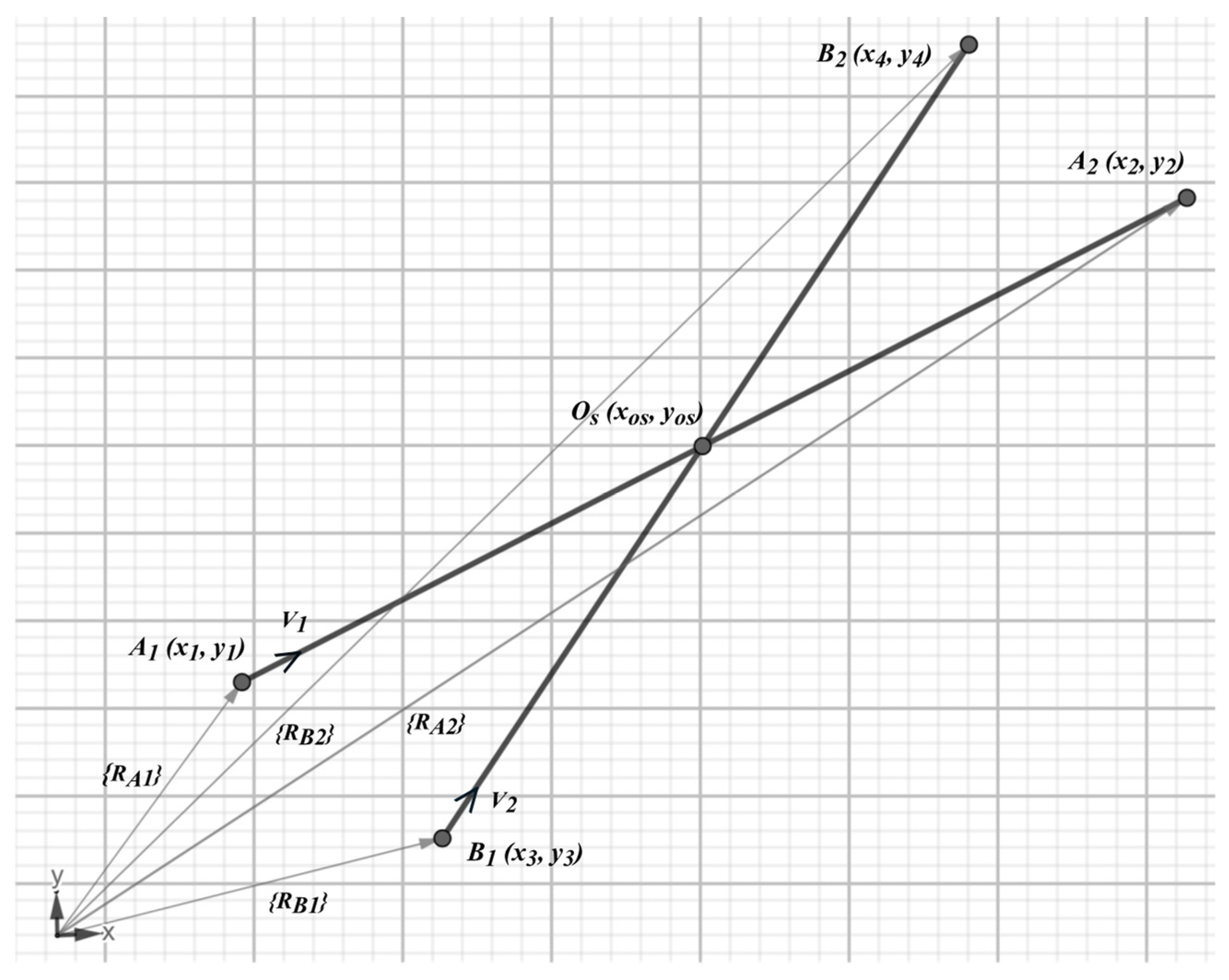
In this paper, we propose to consider two algorithms for resolving conflict situations. The first one assumes that aircraft fly according to the Dubins trajectory; the second one assumes straight-line flight (3HC method). Of the many possible spatial configurations of aircraft involved in a conflict situation, we will analyze the most dangerous case when their distance from the intersection point and flight speed are such that the time of appearance at the collision point is the same. This situation is schematically presented in
Figure 1.
An example of a conflict situation can be described as follows.
In the beginning, one aircraft (marked A) is in point with coordinates . while the other aircraft (marked B) is in point with coordinates .
Destination points, respectively and , determine the flight direction of aircraft.
We assume that both aircraft are in the same control sector and that a minimum separation of 5 nm applies in the examined airspace.
We analyze the problem in two dimensions as we assume that the aircraft fly at the same flight level, which means that a vertical separation of 1000 ft does not apply. Therefore, in further calculations, we will omit the vertical coordinate z.
We will represent the starting and endpoints of both aircraft through vectors
,
,
and
. The trajectories of both aircraft will be denoted by:
where:
The coordinates of the point
, where the trajectories
and
intersect are defined as follows [
46]:
The coordinates of the point , where the trajectories and intersect are one of the primary/fundamental data used for the analysis of our proposed two approaches of conflict resolution algorithms using horizontal maneuvers.
2.1. Dubins Trajectory Method
In geometry, the Dubins trajectory is the shortest curve, which connects two points in the 2D Euclidean plane with the initial and final points and directions specified, or with prescribed initial and terminal tangents to the path [
47,
48]. The Dubins trajectory consists of curves and line segments. The Dubins trajectories are used in the field of robotics and control theory as a way to plan paths for wheeled robots, airplanes, and underwater vehicles [
30,
33].
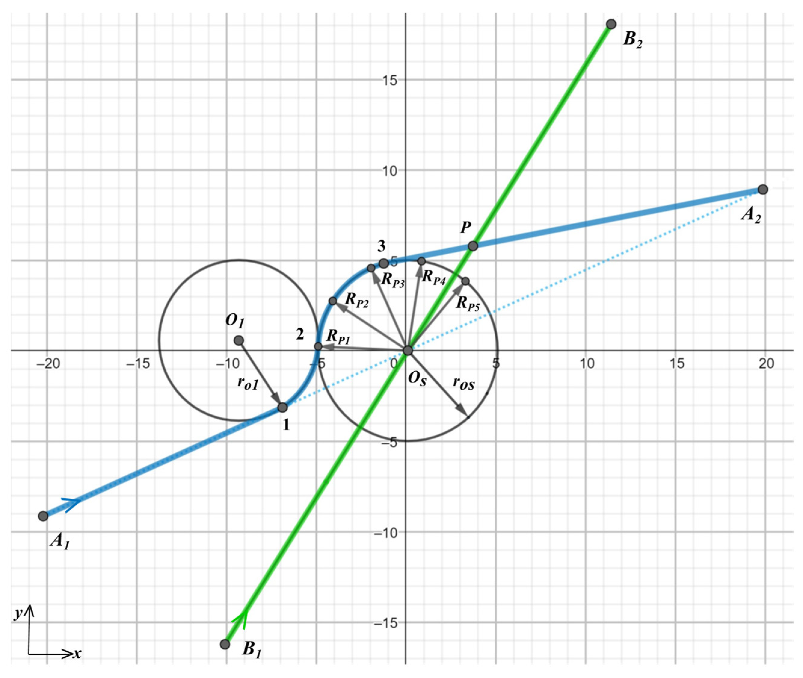
The method of conflict resolution we propose involves changing the flight path of aircraft A, while aircraft B moves according to the initially planned trajectory (
Figure 2).
To determine the Dubins trajectory for aircraft A, we use circles
and
with radii, respectively,
and
. Considering that the movement of aircraft A takes place along the perimeter of the circle
, and the movement of aircraft B through its center, and taking into account the minimum separation used, it was assumed that
. The optimization method presented in
Section 2.3 ensures that primary conflict at point
is not moved to the new conflicting point
(
Figure 2).
The circles
and
determine the characteristic points of the trajectory marked in
Figure 2 by 1, 2, and 3. The way of determining these points is as follows:
- -
Point 1: the point where the trajectory is tangent to the circle ;
- -
Point 2: the point where circle is tangent to the circle ;
- -
Point 3: the point where a straight line passing through point is tangent to the circle .
Thus, the trajectory consists of four parts:
Segment , where is the vector representing point 1;
Arc , connecting points 1 and 2;
Arc , connecting points 2 and 3;
Segment , where is the vector representing point 3.
Tjectory . consists of one segment We assume that both aircraft move at the same speed.
2.1.1. Coordinates of the Characteristic Point 1
The determination of characteristic point 1 is important for both the Dubins and the 3HC methods. At this characteristic point 1, the conflict resolution maneuvers begin. The choice of this point is important both for traffic safety and for extending the flight path. The later aircraft A begins its maneuvers, the smaller the safety margin is as the aircraft approach each other throughout the duration of the conflict; additionally, the sharper the maneuvers will be. On the other hand, the earlier the aircraft starts maneuvers, the greater the increase in route length and the smoother the maneuver. In any case, it must be ensured that the minimum separation is not violated before aircraft A reaches point 1.
We will determine the coordinates of point 1 as follows:
We denote the length of the segment
by
. Then the vector describing the segment
can be represented as follows:
The unit vector
is calculated in the following way:
The denominator of dependence (7) includes the length of the segment
, which we will calculate as follows:
The length
in Formula (6) can be determined as follows:
where, according to Pythagoras’ theorem:
After characteristic point 1, the aircraft proceeds via the designated path towards characteristic point 2.
2.1.2. Coordinates of the Characteristic Point 2
In characteristic point 2, the aircraft starts moving along the perimeter of the circle
. We calculate the vector of coordinates of point 2 in the following way:
We determine vector
of the center of the circle
as follows:
The unit vector
, perpendicular to the segment
can be determined in the following way:
where the normal vector
is equal:
We may determine the unit vector
as follows:
After characteristic point 2, the aircraft proceeds via a designated path towards characteristic point 3.
2.1.3. Coordinates of the Characteristic Point 3
At characteristic point 3, aircraft A terminates the circular motion and begins to move straight down to the trajectory endpoint. We may identify characteristic point 3 as the point where a straight line passing through the point is tangent to the circle . Two cases should be considered.
After characteristic point 3, the aircraft proceeds via a designated path so as to resume the endpoint of trajectory .
2.1.4. Trajectory Length and Flight Duration
After determining all trajectory characteristic points’ coordinates, we determine each segment length and flight duration between characteristic points (
Figure 2).
The trajectory is determined by the sequence of characteristic points
and its length:
is given by Formula (9)
where
where
Assuming that during conflict resolution the aircraft speed is constant, flight time is given by the relationship:
In the absence of a conflict, the flight time would be equal:
where
The additional flight time necessary for aircraft A to solve the conflict situation is:
In this case, then one aircraft flew via the Dubins method for the purpose to resolve a conflict with another one flying via the flight planned route (via unmodified trajectory), the comparison of flight distance and time can be evaluated.
2.2. Triple Heading Change (3HC) Method
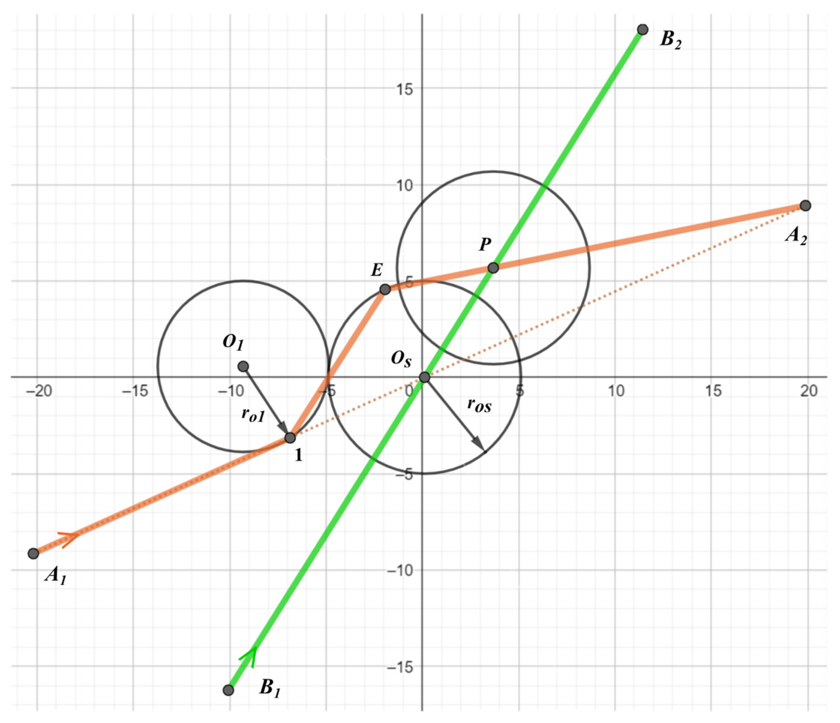
The 3HC method to resolve conflicts within the airborne collision avoidance system was previously described in [
25]. It involves three heading changes of aircraft A to bypass the collision point (
Figure 3). The general algorithm of the 3HC conflict resolution method in a version adapted to the concept presented in this paper is as follows:
At point 1, aircraft A makes a turn in the horizontal plane and starts a flight towards point E,
located on a line perpendicular to the initial flight path of aircraft A at a distance
from the collision point
. This distance is dependent on the position of point 1, the headings, and the flight parameters of both aircraft. We must select it in such a way as to ensure the minimum separation
required by international regulations [
49].
After reaching point , aircraft A makes a second change of heading, starting the flight towards point , i.e., the endpoint of the trajectory .
After reaching point , aircraft A returns to its original heading.
The main problem in the 3HC method is the selection of its parameters, especially the coordinates of point 1 and the radius of the circle
(location of point E). In the paper [
25] we proposed their determination by simulation using a model built on the basis of colored Petri nets.
The aircraft trajectories
and
determined according to the 3HC method are presented in
Figure 3. They can be schematically described as follows:
The coordinates of the vector
we determine as follows:
The unit vector
, perpendicular to the segment
can be determined in the following way:
where the normal vector
is equal:
The flight distance in accordance with the concept of the 3HC method is:
where
we determine with the use of Formulas (8)–(10),
The flight time according to the route consistent with the 3HC method concept is:
In the absence of a conflict, the straight-line flight time between points
and
is:
Therefore, the additional flight time resulting from the need to resolve the conflict, in the case of the 3HC method is:
In this case, then one aircraft flew via the 3HC method for the purpose to resolve a conflict with another one flying via flight planned route (via unmodified trajectory), the comparison of aircraft flight distance and time can be evaluated.
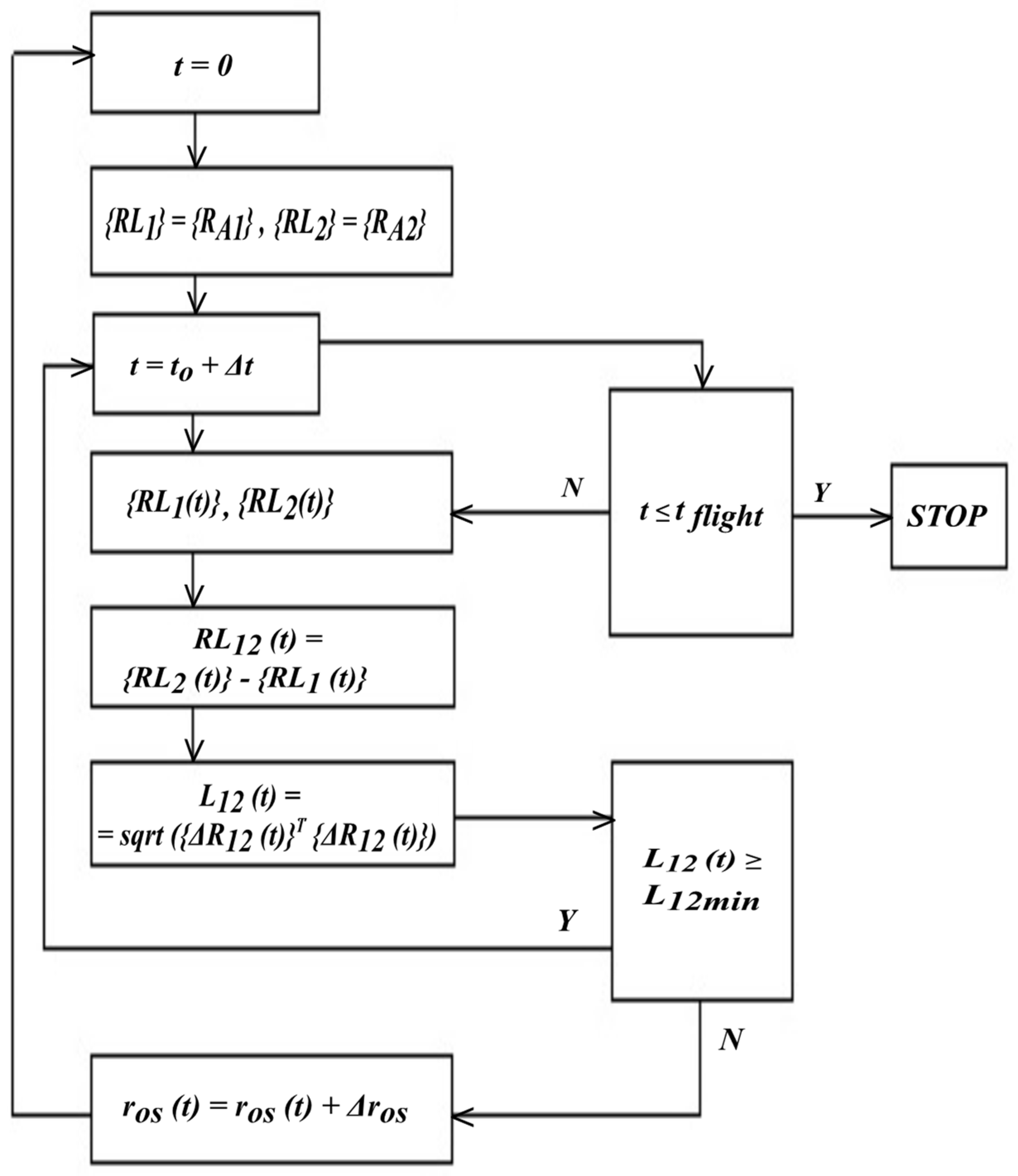
2.3. Optimization Scheme
As has already been mentioned, it is important to select the parameters of the model in such a way that the separation between the aircraft is maintained at any time during the conflict resolution. At the same time, we strive to make as little detour as possible, which takes place when the radius
is as small as possible. For both methods, we selected these parameters by simulation. Its general scheme is shown in
Figure 4.
As the endpoint of the simulation, we choose time , after which both aircraft have passed the destination points and . Throughout the simulation, we monitor the positions (t) and (t) of aircraft A and B, respectively, checking that the minimum separation has not been violated. If at any moment the separation is violated, then we increase the radius (0.1 nm) and repeat the simulation.
2.4. Dubins-like Trajectory Using Non-Circle Curves
In our method using the Dubins trajectory, the aircraft moves along a circular arc. However, in some cases, it may be beneficial that the aircraft follows a different curve, for example, an ellipse. Wanting to include the possibility of determining trajectories not only along the arc, but also along other curves we will determine the coordinates of characteristic points using the parametric approach. In this approach, the
curve, along which the aircraft moves, is a set of points
, approximated using the function
based on five characteristic points
, shown in
Figure 5. The values of function
for those characteristic points are presented in
Appendix A (
Table A1).
where
As in other methods, the most important thing is to determine the characteristic points.
We may determine the
point coordinates’ vector by solving the adequate non-linear equation upon parameter
. For this purpose, we will use the fact that the
vector is tangent to the
circle, so the tangential vector
(
Figure 2) and
are parallel. Thus:
where:
We define function
:
Given the Formula (49) and the fact that
we obtain the equation:
We may solve non-linear Equation (40) upon parameter
numerically using the Newton–Rapson method. In our case, we used the Non-Linear Programming (NLP) solver available in the Maple package. This way we determine the
parameter and thus the
vector:
The
point is located between semicircle points
, determined by vectors
, where
. To determine the
point corresponding to
parameter, we must minimize the non-linear algebraic function:
The is determined in the same way as in the Dubins trajectory.
3. Analysis of the Effectiveness of Two Methods
Using the presented methodology, we compared the proposed methods in terms of their effectiveness in resolving a conflict situation, i.e., when the angles of both trajectories at the starting point of the simulation are 35 and 90 degrees, respectively. We will present this comparison using an example. The coordinates of the starting and ending points (expressed in nautical miles) were adopted as follows:
The speed of the aircraft is
. The coordinates of the conflict point calculated from (53) are as follows:
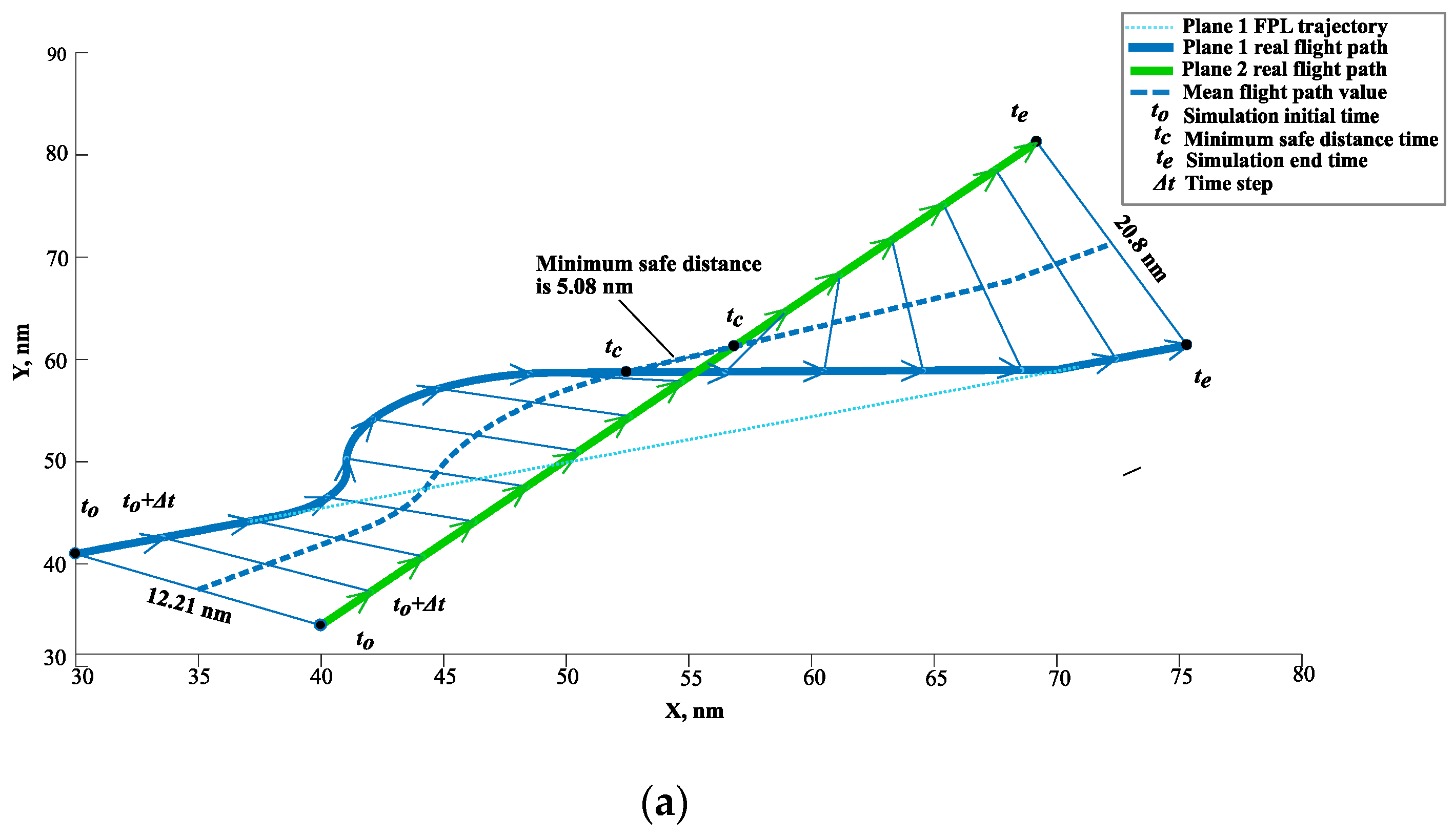
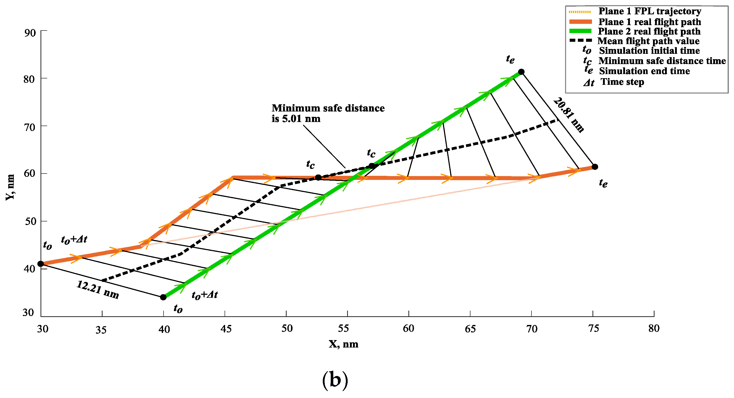
3.1. Conflict Resolution by the Dubins and 3HC Methods (35° Case)
Numerical investigation of the conflict resolution while using the Dubins and the 3HC methods when the angle (for both trajectories) at the starting point of the simulation is 35°, is presented in
Figure 6a (Dubins) and
Figure 6b (3HC).
Both aircraft, as for the Dubins and as for the 3HC variant, fly via upper/left part of the circle with radius .
Using the optimization procedure as discussed in
Section 2.3, numerical investigation results when the angle of both trajectories at the starting point of the simulation is 35° using the Dubins method, show that for such angle between flight trajectories, i.e., 35°, the minimum radius
for which the separation is assured at any moment of the simulation is 8.8 nm. In such a case, the minimum safe distance
between the aircraft is 5.08 nm (detected at 232 s from the beginning of the simulation). Meanwhile, for the 3HC method, it was established that while the angle of both trajectories at the starting point of the simulation is 35°, the minimum radius
for which the separation is assured at any moment of the simulation is 10.10 nm. In this case, the minimum safe distance
between the aircraft is 5.01 nm (detected at 232 s from the beginning of the simulation).
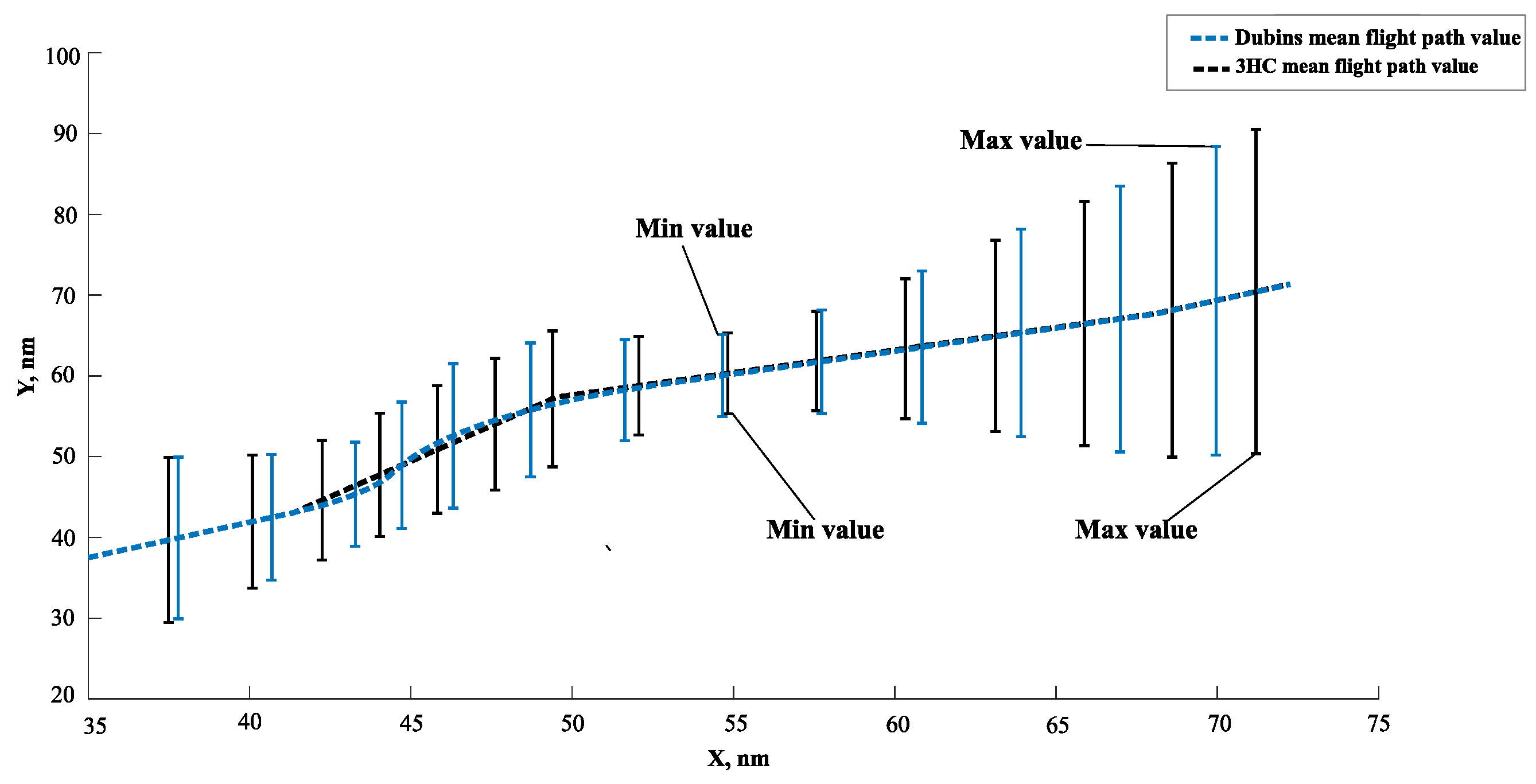
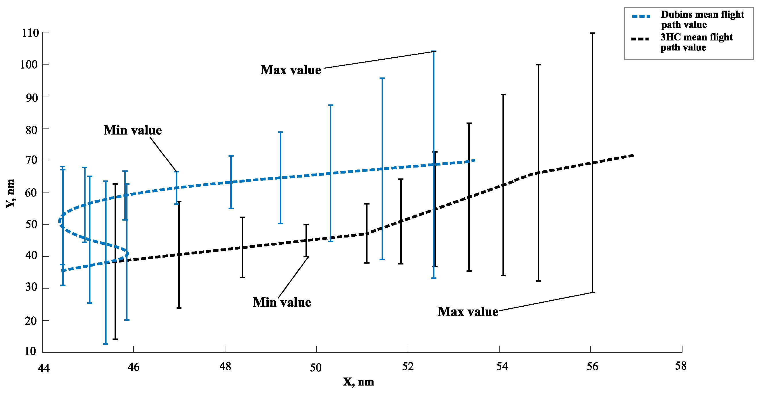
The Dubins and 3HC mean flight path distance values, taking both minimum and maximum values while the angle (for both trajectories) at the starting point of the simulation is 35°, are shown in
Figure 7.
Numerical results for the conflict resolution using the Dubins method when the angle (of both trajectories) at the starting point of the simulation is 35° is slightly more effective than for the 3HC method because the resolution via the Dubins method allows to maintain a minimum safe distance between aircraft at any moment of the flight and to operate via the circle with a smaller radius when resolving the conflict.
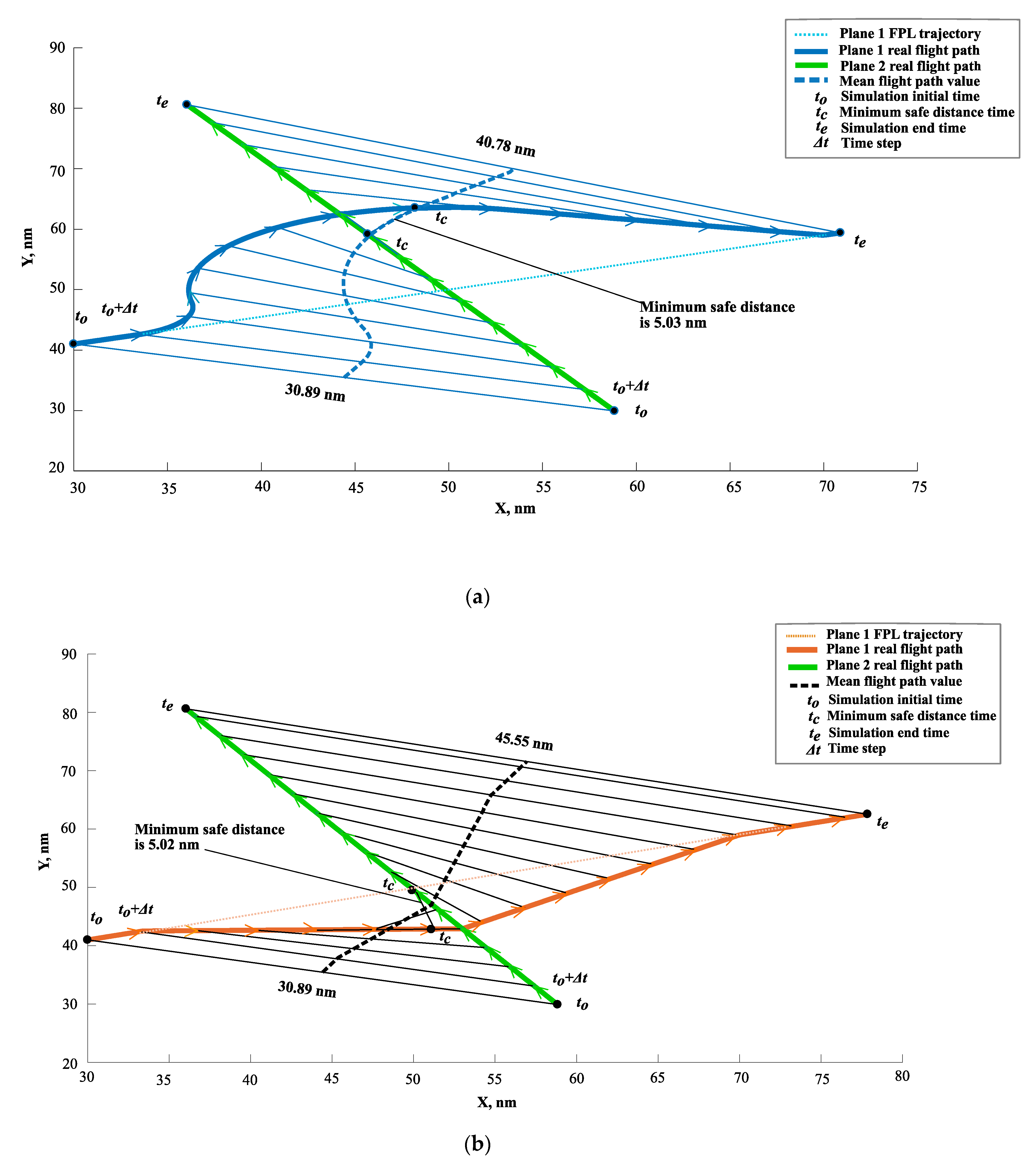
3.2. Conflict Resolution by the Dubins and the 3HC Methods (90° Case)
Numerical investigation of conflict resolution using the Dubins and the 3HC methods of both aircraft (in two dimensions) when the angle (for both trajectories) at the starting point of the simulation is 90°, is presented in
Figure 8a (Dubins) and
Figure 8b (3HC). Moreover, in the Dubins variant, the aircraft flies via the upper part of the circle with a radius
, meanwhile, in the 3HC variant, the aircraft flies via the bottom/right part of the same circle (this was impacted by an initial angle of 90° between the aircraft flight trajectories while the safe and rational solution cannot be found, and due to the constraint that if the radius
value reaches 15 nm, as a logical solution, the aircraft should decide to fly via the bottom part of the circle with a radius
) so as to assure a safe and rational solution.
Using the optimization procedure as discussed in
Section 2.3, numerical investigation results when the angle (for both trajectories) at the starting point of the simulation is 90° using the Dubins method, show that the minimum circle radius
for which the separation is assured at any moment of the simulation is 13.7 nm. In such a case, the minimum safe distance
between the aircraft is 5.03 nm (as detected at 234 s from the beginning of the simulation). Meanwhile, the 3HC method results show that when the angle (for both trajectories) at the starting point of the simulation is 90°, the minimum radius
for which the separation is assured at any moment of the simulation is 7.7 nm. In this case, the minimum safe distance
between the aircraft is 5.02 nm (detected at 136 s from the beginning of the simulation).
The Dubins and 3HC mean flight path distance values, taking both minimum and maximum values when the angle (for both trajectories) at the starting point of the simulation is 90°, are shown in
Figure 9.
Numerical results for conflict resolution using the 3HC method when the angle (for both trajectories) at the starting point of the simulation is 90° are slightly more effective than the Dubins method. The conflict resolution via the 3HC method allows to maintain a minimum safe distance between aircraft at any moment of flight and operate via the circle with a smaller radius while resolving the conflict, i.e., to assure a safe and rational solution.
3.3. The Comparison of the Dubins and the 3HC Methods
The basic criteria for comparing the effectiveness of both methods when the angles (for both trajectories) at the starting point of the simulation are 35° and 90°, respectively, are the time and length of the route traveled by aircraft A in accordance with the adopted trajectory. The results of the comparison are presented in
Table 1 and
Table 2.
It is evident from the results presented for both methods (when the angle (of both trajectories) at the starting point of the simulation is 35°) that they are very similar, but a slightly smaller additional distance has to be covered while using the method of conflict resolution based on the Dubins trajectories.
It is evident that the results of both methods (when the angle (of both trajectories) at the starting point of the simulation is 90°) show that a slightly smaller additional distance is covered while using the method of conflict resolution based on the 3HC method than the Dubins method. It can be explained by the fact that in the case of the 3HC method, optimal is smaller, i.e., 7.7 nm than in the Dubins case, i.e., 13.7 nm. The reason is the angle of 90° between trajectories at the starting point of the simulation where the constraint is set such so that if the radius value reaches 15 nm, as a logical solution, the aircraft should decide to fly via the bottom part of a circle with a radius . Thus, such an interactive optimization allows to reach the solution and assure safe separation between aircraft and produces a shorter route length and time traveled by aircraft.
Another important criterion for evaluating the performance of a conflict resolution method is fuel consumption [
50,
51]. It is usually referred to in relation to a service provided (the number of passengers or ton of freight) and the distance flown. It can be expressed in different ways, for example, by liters of fuel consumed per passenger per kilometer [
52].
As an exemplary aircraft, the long-range Boeing B777-300ER. At Mach 0.839 (481 kts, 891 km/h), flight level FL300, temperature −59 °C and at 513,400 lb (232.9 t) weight, the B777-300ER burns 17,300 lb (7.8 t) of fuel per hour [
53] was chosen. To calculate fuel burn for aircraft using Dubins or 3HC trajectory, we used the Formula (55). In such a way, the total fuel burned per a certain time unit (
Table 3 and
Table 4) was calculated.
As the amount of fuel burn depends on the length and duration of the flight, therefore, while comparing the conflict resolution methods based on the Dubins trajectory and 3HC (when the angle (of both trajectories) at the starting point of the simulation is 35°), very similar results with a minimal advantage of the Dubins method are calculated.
As the amount of fuel burn depends on the length and duration of the flight, therefore, when comparing the conflict resolution methods based on the Dubins trajectory and 3HC (when the angle (for both trajectories) at the starting point of the simulation is 90°), the advantage of the 3HC method against the Dubins method, which can be explained by the facts described above, i.e., the smaller radius , is evident.
4. Conclusions
The aim of the paper was to compare two aircraft conflict resolution methods when the angle (for both trajectories) at the starting point of the simulation is 35° and 90°, respectively.
The analyzes revealed that while the angle (for both trajectories) at the starting point of the simulation is 35°, in the case of the Dubins, the total trajectory length is 49.33 nm, while for the 3HC case, it is 49.55 nm. Thus, the difference in total trajectory length is 0.22 nm, which results in a time difference of t = 1.56 s, and this, in turn, results in smaller fuel consumption of 3.4 kg for the Dubins case. Thus, it can be stated that for such a situation, the Dubins method is slightly more effective. Meanwhile, when the angle (for both trajectories) at the starting point of the simulation is 90°, in the case of the Dubins total trajectory, length is 53.86 nm, while for the 3HC case, it is 46.05 nm. Thus, the difference in total trajectory length is 7.81 nm, which results in a time difference of t = 56.28 s, and this, in turn, results in smaller fuel consumption of 122 kg for the 3HC case. Consequently, it can be stated that for such a situation, the 3HC method is much more effective.
For future research, the conflict resolution effectiveness methods could be extended by changing not only the radius , but the radius , assuring flight centrifugal acceleration is within acceptable limits. In addition, the third aircraft could be taken into consideration as well. Moreover, due regard could be allocated to different aircraft speeds and such uncertainties as wind angle and speed, navigation/positioning errors, etc., and their impact on the effectiveness of the analyzed aircraft conflict resolution concepts.


