Parameter-Matching Algorithm and Optimization of Integrated Thermal Management System of Aircraft

Abstract

The integrated thermal management system of aircraft is essential to maintain a suitable environment for the cabin crew and devices. The system is composed of the air-cycle refrigeration subsystem, the vapor-compression refrigeration subsystem, the liquid-cooling subsystem and the fuel-cycle subsystem, which are coupled with each other through heat exchangers. Due to the complex structure and large number of components in the system, it is necessary to design a corresponding parameter-matching algorithm for its special structure and to select the appropriate optimization design method. In this paper, the structure of an integrated thermal management system is analyzed in depth. A hierarchical matching algorithm of system parameters was designed and realized. Meanwhile, a sensitivity analysis of the system was performed, where key parameters were selected. Besides, a variety of optimization algorithms was used to optimize the design calculations. The results show that the particle swarm optimization and genetic algorithm could effectively find the global optimal solution when taking the fuel penalty as the objective function. Furthermore, the particle swarm optimization method took less time.

1. Introduction

With the development of aviation technology, the aircraft is required to carry high-power equipment, electronic warfare, radar and other advanced avionics components. The overall performance of the electromechanical system needs to be greatly improved and the power-to-weight ratio of the system also needs to be increased [1]. The design of the heat dissipation and heat management systems puts forward more stringent requirements [2], where the mismatch of energy consumption and heat sink is one of the most severe contradictions [3,4]. On the one hand, the aircraft is equipped with a large amount of electromechanical equipment, covering energy conversion, transmission, utilization, etc. During the process, the energy losses are converted into heat loads, which substantially increases the heat-dissipation requirements [5,6]. On the other hand, aircrafts mainly use ram air and fuel as heat sinks [7,8], but technical measures such as the extensive use of composite materials in the aircraft structure, the restriction of the ram-air inlet for stealth and the removal of large energy-consuming bleed air further reduce the available heat sink [9], causing a huge gap in the thermal management of the whole aircraft.

In order to design a better integrated thermal management system for the whole aircraft, it is necessary to analyze various heat-generating components on the aircraft and the elements of the thermal management system. Generally, energy-generating components and executive equipment are distributed in different parts of the aircraft. The environment, surface heat-dissipation characteristics, operation conditions and mission profiles must be considered in the thermal load modeling and temperature prediction control [10]. The aircraft electromechanical system includes relatively independent sub-systems, such as electrical system, hydraulic system, fuel system and environmental control system; their transmission and utilization are closely related if analyzed from the perspective of energy and heat flow. Therefore, it is necessary to change the design concept from the optimization of individual subsystems to the optimization of the entire system. Walters et al. [11] established the interface control and specification document for advanced modeling and simulation and realized the analysis and optimization of the system by integrating subsystem models. Further, Donovan [12] used the tip-to-tail model to simulate the overall thermal management system of the whole aircraft, which realizes the optimal design of the system and meets the heat-dissipation requirements of the integrated airborne electromechanical system.

For a simple thermal system, all the characteristic equations of each component can be simultaneously solved to obtain the air state parameters at each point of the system. However, for the integrated thermal management system, the structure is more complicated. The system contains tens of components and state points. Each state point contains temperature, pressure, humidity, specific enthalpy and other parameters [13]. At the same time, the system includes calculation equations for physical parameters of air and coolant, module and component characteristic equations, connection equations and other constrained equations. Some of them are nonlinear equations and the solution is complicated. Therefore, it is difficult to solve them directly by the method of simultaneous equations. In order to ensure the correctness of the calculation and reduce the possibility of errors, it is necessary to design the corresponding calculation process or framework for the special structure of the integrated thermal management system. Researchers have sought various methods to solve this problem. For the thermal management system of electric aircrafts, Freeman et al. [14] designed a process for calculating the total take-off weight and developed a corresponding optimization program, which mainly focuses on the thermal management system and its integration within the propulsion system. Doman [15] determined the optimal thermal cruise conditions for jet aircrafts by deriving and solving sets of ordinary differential equations.

Besides, the thermal management system involves many variables. If the variables are directly used to optimize the design, it leads to excessive calculations and lower calculation efficiency [16]. In addition, it is easier to cause the cost function to fall into a local extremum point during optimization. In this case, it is hard to find the global optimal solution [17]. Jiang et al. [18] carried out a sensitivity analysis for the ACS, obtained key parameters and simplified the optimization design process. The process can greatly reduce the calculation time. Therefore, for integrated thermal management systems, it is necessary to analyze the parameters that have a greater impact during the process based on the parameter-matching calculation. The analysis process is helpful in reducing the complexity of optimization calculation.

To address the difficulty in the parameter matching of the system and to speed up the process of optimization, this paper proposes an optimization process for the aircraft thermal management system with three steps. First, the structure of the integrated thermal management system was analyzed in depth and the multi-level matching calculation of the system parameters was designed and realized. Then, the sensitivity analysis of the system parameters was carried out, where key parameters were chosen to reduce the number of optimization variables. Lastly, a variety of optimization algorithms were used for optimization design calculations, where different numbers of optimization variables were selected to compare the results.

2. Structure of the Integrated Thermal Management System

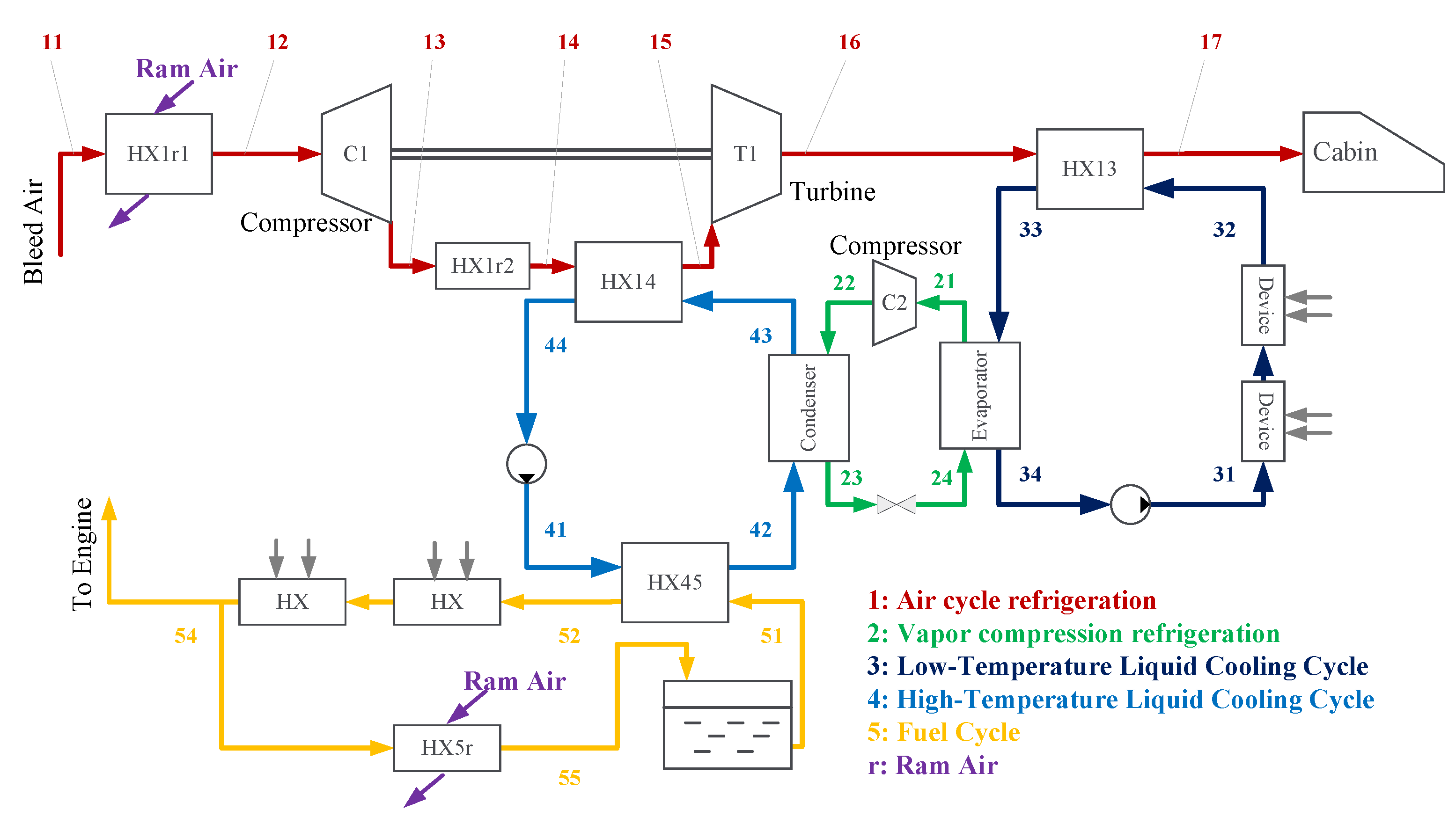
The integrated environmental control system mainly includes the air-cycle refrigeration subsystem (ACS), the vapor-compression refrigeration subsystem (VCS), the liquid-cooling-cycle subsystem and the fuel-cycle subsystem. The structure of the integrated environmental control system is shown in Figure 1.

The cabin of aircrafts requires air ventilation; thus, it uses an ACS to provide suitable pressure and temperature air. Meanwhile, low-power electronic equipment also uses air as the cooling medium. For high-power electronic equipment, the low-temperature liquid-cooling cycle is used to transfer the heat to the VCS and then to the high-temperature liquid-cooling cycle; the fuel is used as the final heat sink.

These five subsystems are coupled with each other through heat exchangers to achieve the goal of thermal management. The functions of each subsystem are detailed below.

• The air-cycle refrigeration subsystem
  Due to the relatively small thermal load generated by the cabin, crew and low-power electronic equipment, the ACS can meet the needs of regulating temperature and pressure. The type of ACS is two-wheel bootstrap [19]. The high-temperature air bleeding from the engine compressor enters the subsystem, passes through the primary air heat exchanger and enters the compressor. The air with high temperature and pressure from the compressor enters the secondary heat exchanger and the heat exchanger, which are coupled with the high-temperature liquid-cooling-cycle subsystem, then expands in the turbine. Finally, the air passes through the heat exchanger coupled with the low-temperature liquid-cooling-cycle subsystem and, finally, flows to the cabin at a suitable temperature and pressure.
• The vapor compression refrigeration subsystem
  The onboard VCS uses R134a as the refrigerant [20]. The refrigerant R134a evaporates in the evaporator, absorbing the heat of the liquid-cooling working fluid in the low-temperature liquid-cooling cycle. The gaseous R134a from the evaporator enters the compressor. By receiving the work of the compressor, the temperature and pressure of the refrigerant increase. After that, the refrigerant enters the condenser. In the condenser, the R134a with high temperature transfers heat to the working fluid of the high-temperature liquid-cooling-cycle subsystem. Subsequently, the temperature of R134a decreases and cools down into a liquid state. Later, the refrigerant flows through the throttle valve, which can be described as an isenthalpic process with its pressure and temperature decreasing. After that, the refrigerant flows back into the inlet of compressor.
• The low-temperature liquid-cooling-cycle subsystem
  The cooling capacity of the equipment can be generated by the VCS, but it also needs a liquid cycle to transfer the heat between equipment and the VCS. Liquid cooling is usually adopted for the cooling of the circuit board of the high-power integrated electronic equipment cabin. In this subsystem, high-power electronic equipment is directly connected to the low-temperature liquid-cooling cycle. Driven by the pump, the low-temperature liquid-cooling cycle absorbs the heat load from the electronic cabin and transfers the heat to the VCS in the evaporator.
• The high-temperature liquid-cooling-cycle subsystem
  In the high-temperature liquid-cooling-cycle subsystem, the working fluid is driven by a pump and passes through multiple heat exchangers. The condenser of the VCS, the secondary heat exchanger of the ACS and the liquid-cooled heat exchanger of the fuel cycle are connected in sequence to transfer heat to the fuel-cycle subsystem. The fuel is used as a heat sink to take the heat away.
• The fuel-cycle subsystem
  In the integrated thermal management system, the fuel-cycle subsystem mainly involves (1) the heat exchanger between the fuel and the high-temperature liquid-cooling cycle; (2) the heat exchanger between the fuel and the thermal load of the secondary power system (SPS), including lubricating oil cycle and hydraulic oil cycle; and (3) the heat exchanger between fuel and ram air. Among them, the heat exchanger No.2 is simplified to take the thermal load as a design variable.

3. System Parameter Matching

3.1. Hierarchical Parameter-Matching Algorithm

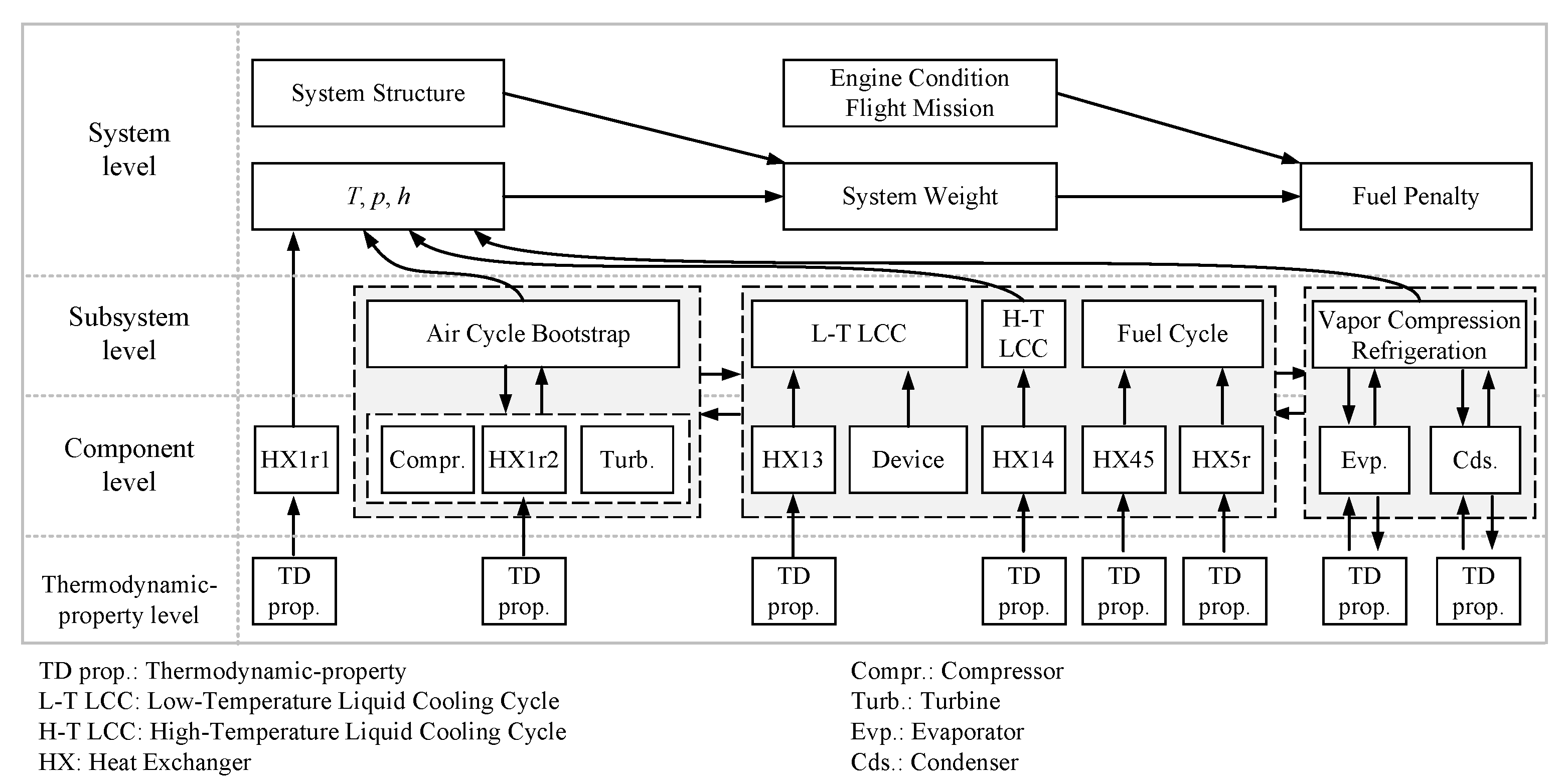
The system structure of the integrated thermal management system is typically hierarchical. According to the structural characteristics of the system, the parameter-matching process can be divided into four levels, namely, system level, subsystem level, component level and thermodynamic-property level. The general planning of the parameter-matching calculation process of the integrated thermal management system is shown in Figure 2.

• System level
  At the system level, the total weight of the system can be calculated according to the system structure configuration. Then, the fuel penalty can be calculated from the temperature, pressure, humidity, specific enthalpy and other parameter values of each state point, combined with engine performance parameters and flight conditions.
• Subsystem level
  The integrated thermal management system consists of subsystems such as the ACS, the VCS, the liquid-cooling-cycle subsystem and the fuel-cycle subsystem. As the working fluids of each subsystem are not the same, matching calculations need to be performed according to the characteristics of their respective subsystems. After the component calculation is completed, results are returned to the upper system parameter calculation.
  For the ACS, the core part is the turbine-compressor bootstrap component. Therefore, the calculation of this subsystem mainly covers turbines, compressors and a series of heat exchangers related to them, including secondary ram-air heat exchanger and the heat exchanger between the ACS and high-temperature liquid-cooling cycle. For the VCS, the calculation of the high-temperature liquid-cooling cycle and the low-temperature liquid-cooling cycle determine the heat exchange of its evaporator and condenser during system parameter-matching calculations. Then, the capacity of performance (COP) of the VCS can be obtained.
• Component level
  At the component level, the parameters of air, coolant and fuel at the inlet and outlet can be calculated through the characteristic equations of each component. After the calculation of each component, the results are returned to the subsystem level. In particular, the calculation of components, such as the primary heat exchanger, does not need iteration related to other components or subsystems. The results can be directly passed to the system level after the calculation.
• Thermodynamic-property level
  In the thermal management system, the parameters of most major components can be directly calculated and obtained without iterative calculations. Iterative calculations are necessary only when the phase-change process is involved and the saturation state needs to be determined. The state points where calculations are required are located in the VCS. At the thermodynamic-property level, only the enthalpy of the fluid is known, while the pressure, temperature and specific entropy are coupled with each other. Therefore, the results of the parameters can be solved by constructing a set of equations among the three parameters.

3.2. Conditions and Assumptions

The system parameter-matching design model can be constructed based on the structure of the integrated thermal management system and analysis of various components of the system. Furthermore, the fuel penalty of the system is calculated as the objective function of the following optimization: For parameter matching during system design, the efficiency of each component is given. During this process, the parameters of air, coolant and fuel at each key point are calculated. Finally, a complete design scheme is obtained.

When designing an integrated thermal management system, the following parameters are usually considered as known:

• Engine performance parameters, including outlet temperature and pressure parameters of the compressor, bleed air conditions, etc.;
• Flight parameters, including flight Mach number, time and altitude, to determine the ambient temperature and pressure;
• Cabin-air-supply parameters, including air-supply flow rate, temperature and pressure;
• Engine-fuel-supply parameters, including fuel-supply flow rate and fuel temperature;
• Thermal load parameters, including heat generation of electronic equipment, heat generation of secondary power systems, etc.

In order to simplify the parameter-matching process, the following assumptions were made:

• Ignoring the humidity of air, dry-air properties were used for calculations [21];
• Ignoring the dynamic process of fuel tanks and pipes, only steady-state conditions were considered [21];
• The heat generated by liquid-cooling pumps and fuel pumps were ignored;
• The resistance of the pipeline was considered in neighboring components;
• We assumed that the pressure drop ratio of the heat exchanger was constant [22];
• The thermodynamic properties of the working fluid were considered to be constant [21].

3.3. Parameter-Matching Calculation Process

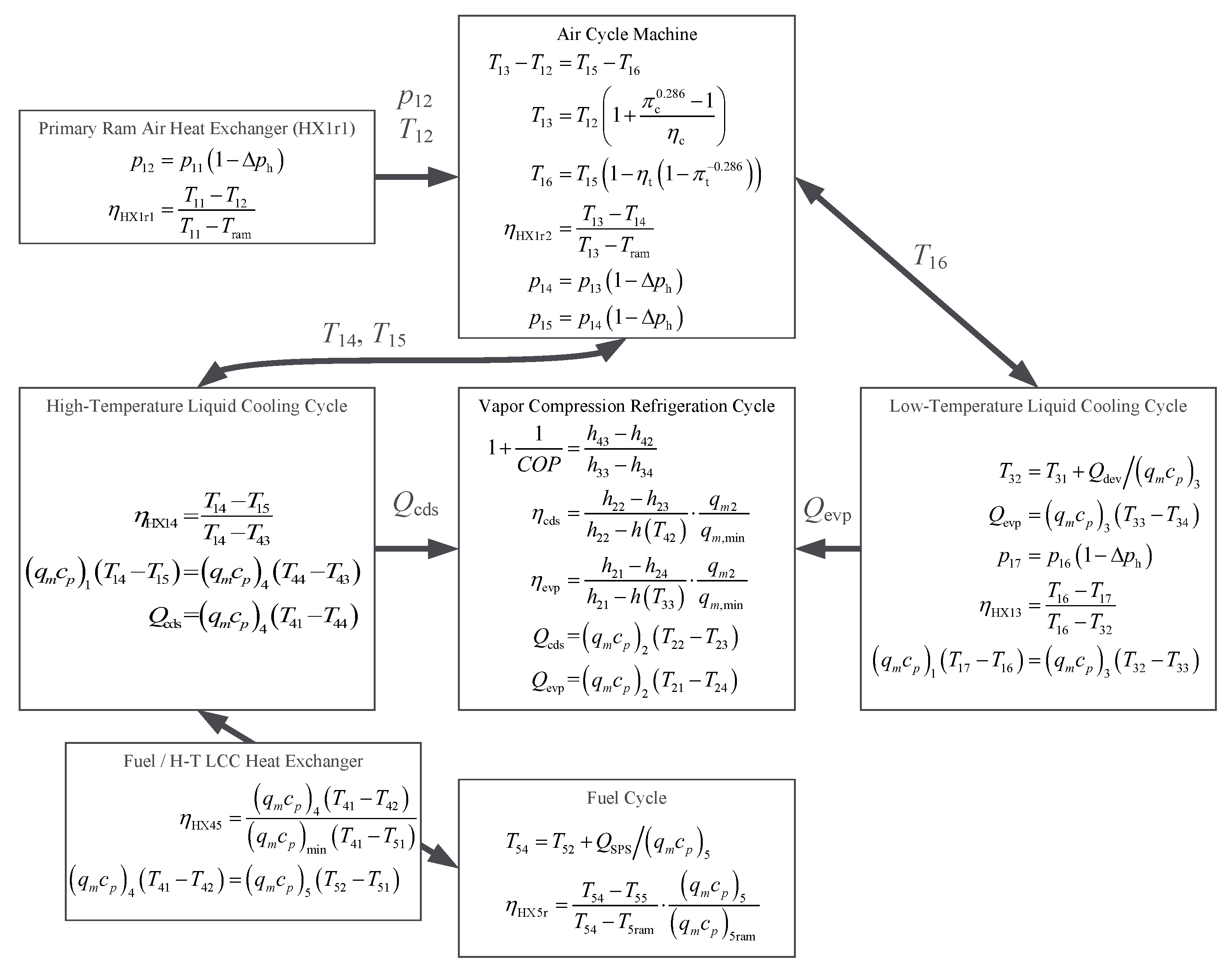
As analyzed above, the structure of a thermal management system is typically hierarchical. The parameters are matched according to the thermodynamic-property–component–subsystem–system scheme. At the thermodynamic-property calculation level, the corresponding temperature and specific enthalpy are calculated according to the specific heat capacity of each point. At the component calculation level, the calculation of the heat-exchanger efficiency and heat-transfer balance processes are the main concern. At the subsystem calculation level, the parameters are calculated according to the characteristics of each subsystem. For the ACS, the main calculation includes the turbine-compressor component; for the VCS, the calculation of the refrigeration cycle and energy efficiency calculations under a given cooling capacity is important. At the system calculation level, according to the parameters of each key point and component, system-level parameters such as the total mass and fuel penalty of the system can be calculated.

According to the structure of the thermal management system model and the characteristic equations of each component, the framework of the parameter-matching algorithm was designed according to the structural composition and the degree of correlation, which was deemed convenient for the following analysis and the design of the specific algorithm flow. The algorithm framework was divided into several parts and each part was solved independently, but, at the same time, each part has some connection with the outside components, as shown in Figure 3.

As can be seen from Figure 3, despite the complex structure of the thermal management system, it can be divided into several parts through analysis. Each part is composed of one or more components, which are coupled by transferring temperature and heat flow. The data transfer among various parts might be unidirectional or bidirectional. Therefore, the sequence of calculations needs to be considered. For the interior of each part, it is necessary to construct an iterative process to solve the parameters according to the characteristics of the components of each part.

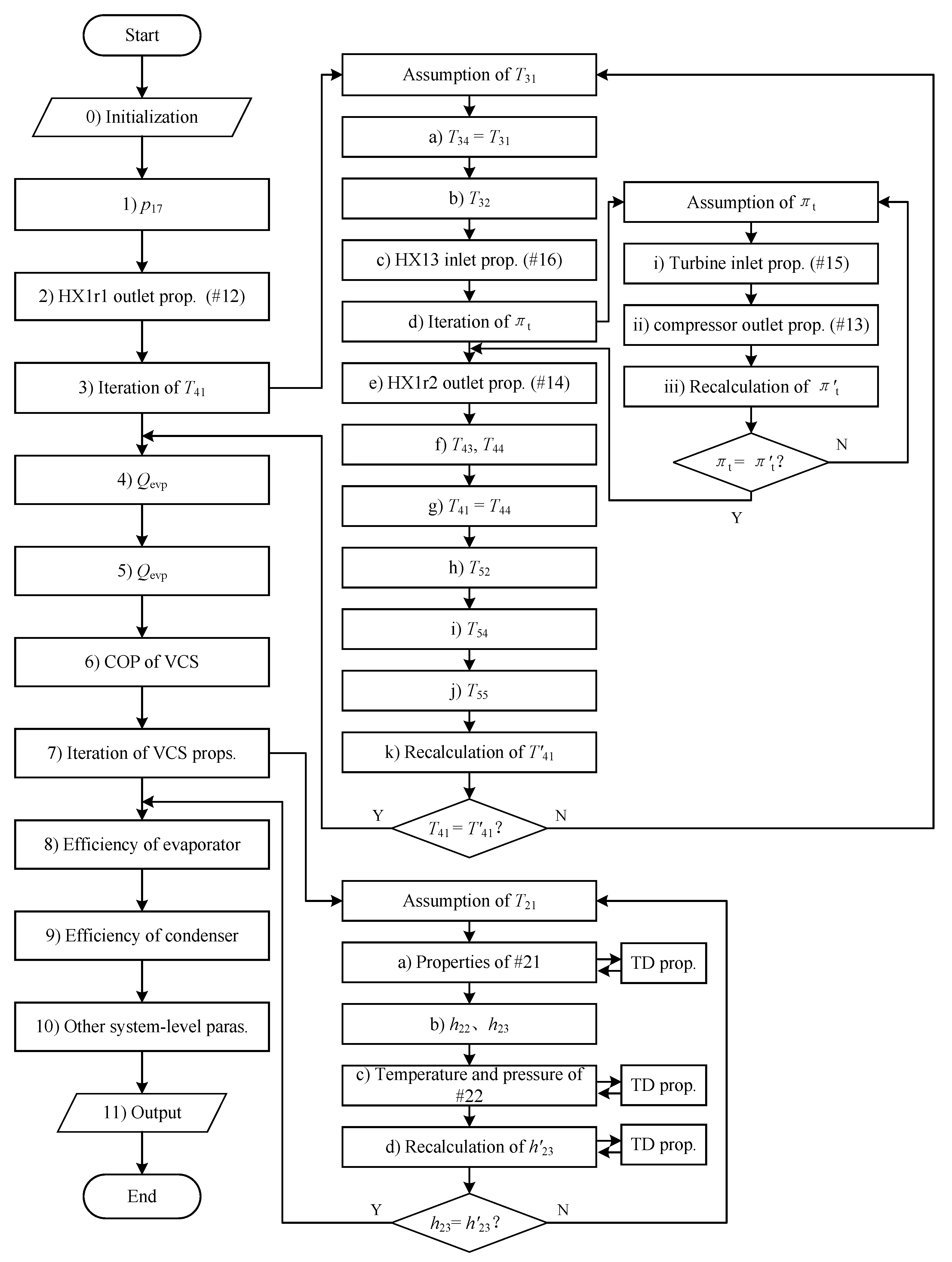
Furthermore, according to the parameter-matching algorithm framework of the above-mentioned preliminary designed thermal management system and the specific characteristic equations of each component, an algorithm flow that is suitable for computer programming was designed as shown in Figure 4.

According to the system parameter-matching calculation process, the specific calculation steps are as follows:

• $p_{16}$ is calculated according to the pressure of the cabin supply air $p_{17}$.

  $$p_{16}=\frac{p_{17}}{1-\Delta p_h}$$

  (1)
• The outlet temperature and pressure of the heat exchanger HX1r1 ($T_{12}$ and $p_{12}$) are calculated according to the temperature and pressure of the bleed air [23].

  $$T_{12}=T_{11}-{\eta }_{HX1}\left(T_{11}-T_{ram}\right)$$

  (2)

  $$p_{12}=p_{11}\left(1-\Delta p_h\right)$$

  (3)
• The outlet temperature of the pump in the low-temperature liquid-cooling cycle is assumed as $T_{31}$.

  (a)

  Ignoring the temperature change of the fluid in the pump, $T_{34}=T_{31}$.

  (b)

  The circulating liquid absorbs the heat from the electronic equipment and the temperature rises.

  $$T_{32}=T_{31}+\frac{Q_{dev}}{q_{m3}{c}_{p3}}$$

  (4)

  (c)

  According to the energy balance and the formula of heat-exchanger efficiency, the air-side inlet temperature $T_{16}$ of the heat exchanger HX13 is calculated.

  $$T_{16}=\frac{T_{17}-{\eta }_{HX13}{T}_{32}}{1-{\eta }_{HX13}}$$

  (5)

  (d)

  Assuming the turbine pressure ratio ${\pi }_t$, we perform the following iterative calculation:

  • Calculate the turbine inlet pressure and temperature, $p_{15}$ and $T_{15}$ [24].

    $$p_{15}=p_{16}·{\pi }_t$$

    (6)

    $$T_{15}=\frac{T_{16}}{1-{\eta }_t\left(1-{\pi }_t^{-0.286}\right)}$$

    (7)
  • Calculate the compressor outlet temperature $T_{13}$, according to the energy balance.

    $$c_p(T_{13}-T_{12})=c_p(T_{15}-T_{16})$$

    (8)
  • Calculate the pressure ratio of compressor and recalculate the turbine expansion ratio [24].

    $${\pi }_c={\left[\left(\frac{T_{13}}{T_{12}}-1\right){\eta }_c+1\right]}^{3.5}$$

    (9)

    $${\pi }_t^{\prime }=\frac{p_{12}}{p_{16}}{\pi }_c{\left(1-\Delta p_h\right)}^2$$

    (10)
  • Compare the result with the assumed turbine pressure ratio; return to recalculate if not matched.

  (e)

  Calculate the air-side outlet temperature $T_{14}$ of the heat exchanger HX1r2.

  $$T_{14}=T_{13}-{\eta }_{HX1r2}\left(T_{13}-T_{ram}\right)$$

  (11)

  (f)

  Calculate the liquid-side outlet temperature of the heat exchanger HX14 ($T_{43}$ and $T_{44}$).

  $$T_{43}=T_{14}-\frac{T_{14}-T_{15}}{{\eta }_{HX14}}$$

  (12)

  $$T_{44}=T_{43}+\frac{{\left(q_m{c}_p\right)}_1}{{\left(q_m{c}_p\right)}_4}\left(T_{14}-T_{15}\right)$$

  (13)

  (g)

  Ignoring the temperature change of the liquid-cooling pump, $T_{41}=T_{44}$.

  (h)

  Calculate the fuel temperature $T_{52}$ before absorbing the heat generated by the secondary energy system.

  $$T_{52}=T_{54}-\frac{Q_{SPS}}{{\left(q_m{c}_p\right)}_5}$$

  (14)

  (i)

  Calculate the fuel temperature after the ram-air heat exchanger ($T_{55}$).

  $$T_{55}=T_{54}-{\eta }_{HX5r}\left(T_{54}-T_{ram}\right)\frac{{\left(q_m{c}_p\right)}_{5,ram}}{{\left(q_m{c}_p\right)}_5}$$

  (15)

  (j)

  Recalculate the inlet temperature of the coolant side of the heat exchanger HX45 ($T_{41}^{\prime }$), according to the conservation of energy.

  $$T_{41}^{\prime }=\frac{{\left(q_m{c}_p\right)}_5\left(T_{52}-T_{51}\right)}{{\left(q_m{c}_p\right)}_4}+T_{42}$$

  (16)

  (k)

  Compare $T_{41}$ and $T_{41}^{\prime }$; return to assume $T_{31}$ again if not matched.

• Calculate the heat exchange of the evaporator.

  $$Q_{cds}={\left(q_m{c}_p\right)}_4\left(T_{43}-T_{42}\right)$$

  (17)
• Calculate the heat exchange of the condenser.

  $$Q_{evp}={\left(q_m{c}_p\right)}_3\left(T_{33}-T_{34}\right)$$

  (18)
• Calculate the COP of the VCS.

  $$COP={\left(1-\frac{Q_{cds}}{Q_{evp}}\right)}^{-1}$$

  (19)
• Assume the outlet temperature $T_{21}$ of the evaporator.

  (a)

  Calculate the specific enthalpy $h_{21}$, specific entropy $s_{21}$ and pressure $p_{21}$ of point 21, according to the thermodynamic properties of the refrigerant.

  (b)

  Calculate $h_{22}$ and $h_{23}$ according to the heat exchange of evaporator and condenser.

  $$h_{23}=h_{21}-Q_{evp}/q_{m2}$$

  (20)

  $$h_{22}=h_{23}+Q_{cds}/q_{m2}$$

  (21)

  (c)

  Calculate $T_{22}$ and $p_{22}$ according to the thermodynamic properties of the refrigerant.

  (d)

  Let $p_{23}=p_{22}$; recalculate $h_{23}^{\prime }$ according to $p_{23}$

  (e)

  Compare $h_{23}$ and $h_{23}^{\prime }$; return and assume $T_{21}$ again if not matched.

• Calculate the efficiency of the evaporator.

  $${\eta }_{evp}=\frac{h_{21}-h_{24}}{h_{21}-h_{33}}·\frac{q_{m2}}{q_{m,min}}$$

  (22)
• Calculate the efficiency of the condenser.

  $${\eta }_{cds}=\frac{h_{22}-h_{23}}{h_{22}-h_{42}}·\frac{q_{m2}}{q_{m,min}}$$

  (23)

In the calculation process described above, in order to ensure the completeness of the parameter calculation process, the thermodynamic properties of the working fluids need to be known in advance.

Besides, the following 11 design parameters need to be selected:

• ${\eta }_{HX1r1}$: Efficiency of ACS’s primary HX
• ${\eta }_{HX1r2}$: Efficiency of ACS’s secondary HX
• ${\eta }_{HX13}$: Efficiency of air/low-temperature liquid-cooling HX
• ${\eta }_{HX14}$: Efficiency of air/high-temperature liquid-cooling HX
• ${\eta }_{HX45}$: Efficiency of fuel/high-temperature liquid-cooling HX
• ${\eta }_{5r}$: Efficiency of fuel/ram-air HX
• ${\eta }_c$: Efficiency of ACS’s compressor
• ${\eta }_t$: Efficiency of ACS’s turbine
• $q_{m3}$: Flow rate of low-temperature liquid-cooling cycle
• $q_{m4}$: Flow rate of high-temperature liquid-cooling cycle
• $q_{m5}$: Flow rate of fuel cycle

According to the results of parameter-matching calculations, other system parameters can be calculated and the fuel penalty of the whole system can be obtained after parameter matching is finished. The results can provide data for sensitivity analyses and optimization calculations.

3.4. Results of Parameter Matching

The parameter-matching process was realized using MATLAB code.

For a certain aircraft, there are several states during flight. Usually, the ground maximum state corresponds to the harshest conditions and the cruise may last the longest time. Therefore, to estimate the performance of the integrated thermal management system, we should pay attention to these two conditions. The parameters and flight conditions are shown in

Table 1. Design parameters of system.

Parameters	Ground	Cruise
Supply air temperature of the cabin	266 K	266 K
Supply air pressure	101 kPa	80 kPa
Flow rate of cabin supply air	0.2 kg/s	0.2 kg/s
Heat of electronic device	50 kW	50 kW
Heat of secondary energy system	40 kW	40 kW
Supply fuel temperature of engine	343 K	343 K
Flow rate of supply fuel of engine	0.3 kg/s	0.2 kg/s
Ram-air total temperature	288 K	267 K
Flow rate of low-temperature liquid-cooling cycle	1.25 kg/s	0.8 kg/s
Flow rate of high-temperature liquid-cooling cycle	2.22 kg/s	1.67 kg/s

.

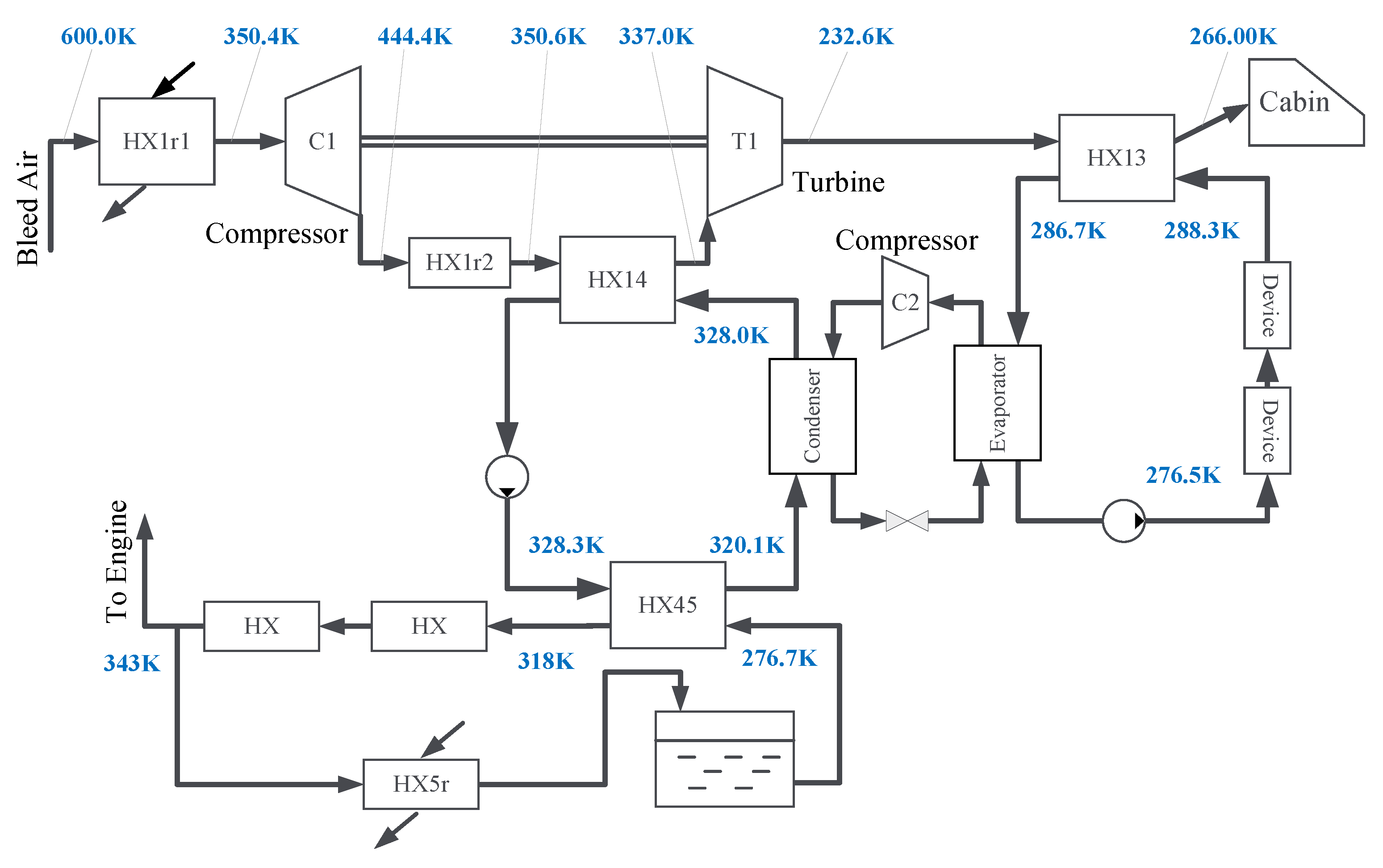
For comparison, we also developed codes in Engineering Equation Solver (EES), which is commercial software for solving common equations. The pressure and temperature results for the two conditions are shown in

Table 2. Results of parameter matching.

	Ground State			Cruise State
	MATLAB	EES	Difference	MATLAB	EES	Difference
$p_{11}$	350.00	350.00	0.000%	350.00	350.00	0.000%
$p_{12}$	348.30	348.25	0.014%	348.30	348.25	0.014%
$p_{13}$	661.10	661.62	−0.078%	636.00	636.53	−0.083%
$p_{14}$	657.70	658.31	−0.093%	632.90	633.35	−0.071%
$p_{15}$	654.50	655.02	−0.079%	629.70	630.18	−0.076%
$p_{16}$	101.50	101.51	−0.007%	80.40	80.40	−0.002%
$p_{17}$	101.00	101.00	0.000%	80.00	80.00	0.000%
$T_{11}$	600.00	600.00	0.000%	600.00	600.00	0.000%
$T_{12}$	350.40	350.40	0.000%	423.00	423.00	0.000%
$T_{13}$	444.40	444.42	−0.005%	529.00	529.06	−0.012%
$T_{14}$	350.60	350.57	0.009%	387.50	387.53	−0.008%
$T_{15}$	337.00	337.02	−0.007%	353.10	353.07	0.009%
$T_{16}$	232.60	232.55	0.021%	235.20	235.22	−0.009%
$T_{17}$	266.00	266.00	0.000%	266.00	266.00	0.000%
$T_{31}$	276.50	276.54	−0.015%	274.70	274.76	−0.023%
$T_{32}$	288.30	288.30	0.001%	286.50	286.52	−0.007%
$T_{33}$	286.70	286.72	−0.006%	285.00	285.07	−0.023%
$T_{41}$	328.30	328.33	−0.010%	331.20	331.25	−0.014%
$T_{42}$	320.10	320.07	0.010%	317.10	317.12	−0.005%
$T_{43}$	328.00	327.99	0.002%	330.10	330.09	0.002%
$T_{51}$	276.70	276.67	0.011%	265.00	265.01	−0.005%
$T_{52}$	318.00	318.00	0.000%	318.00	318.00	0.000%
$T_{54}$	343.00	343.00	0.000%	343.00	343.00	0.000%

Pressure unit, kPa; temperature unit, K.

. We can see from the table that the results calculated from MATLAB and EES are very close. However, EES required a good initial guess for every variable.

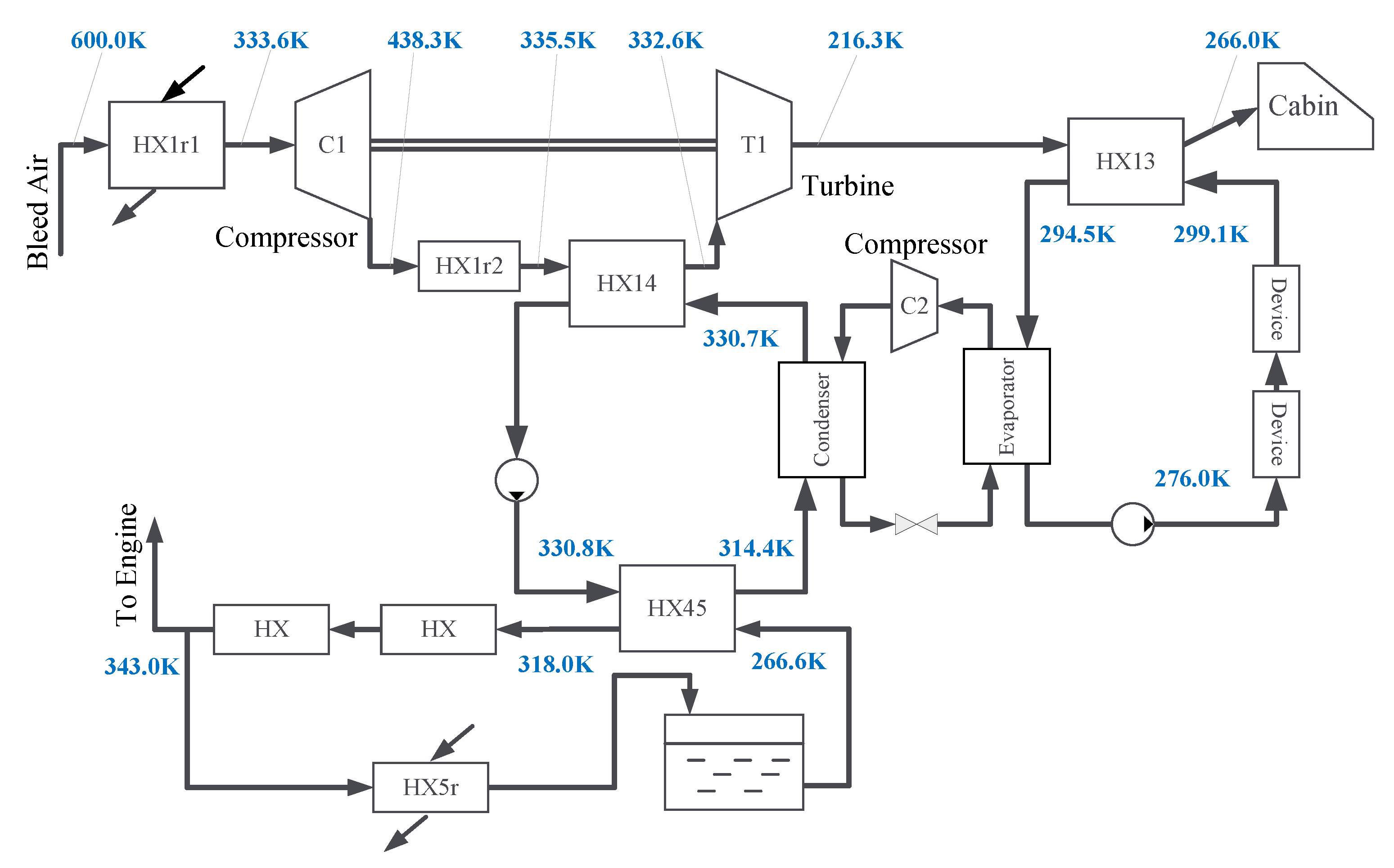
For better intuition, the temperature results were also marked in the system scheme diagrams, as shown in Figure 5 and Figure 6.

Under cruise conditions, the supply air pressure is lower; thus, it needs a higher pressure ratio of the turbine, while the cooling capacity of ACS is higher than that under ground conditions. Therefore, the flow rate of the liquid-cooling cycle and the power of VCS are also lower.

The results show that the algorithm could perform parameter matching with a wide range of input data, covering different stages of flight.

3.5. Fuel Penalty Calculation

The total weight of the aircraft increases after it is equipped with a thermal management system. Besides, ram air, bleed air and power extracted from the engine also cause energy loss. To quantitatively describe the impact of these factors on aircraft flight performance, they can be converted into the increment of fuel consumption, which is also called the fuel penalty method. In this paper, fuel penalty is used as the objective function for further optimization.

The fuel penalty $m_f$ is comprised of four parts, i.e., system device mass $m_{f,dev}$, ram-air resistance $m_{f,ram}$, engine power extraction $m_{f,P}$ and engine bleed air $m_{f,bl}$.

$$m_f=m_{f,dev}+m_{f,ram}+m_{f,P}+m_{f,bl}$$

(24)

The detailed calculation process of each part is shown in Appendix A.

3.6. Sensitivity Analysis of Fuel Penalty

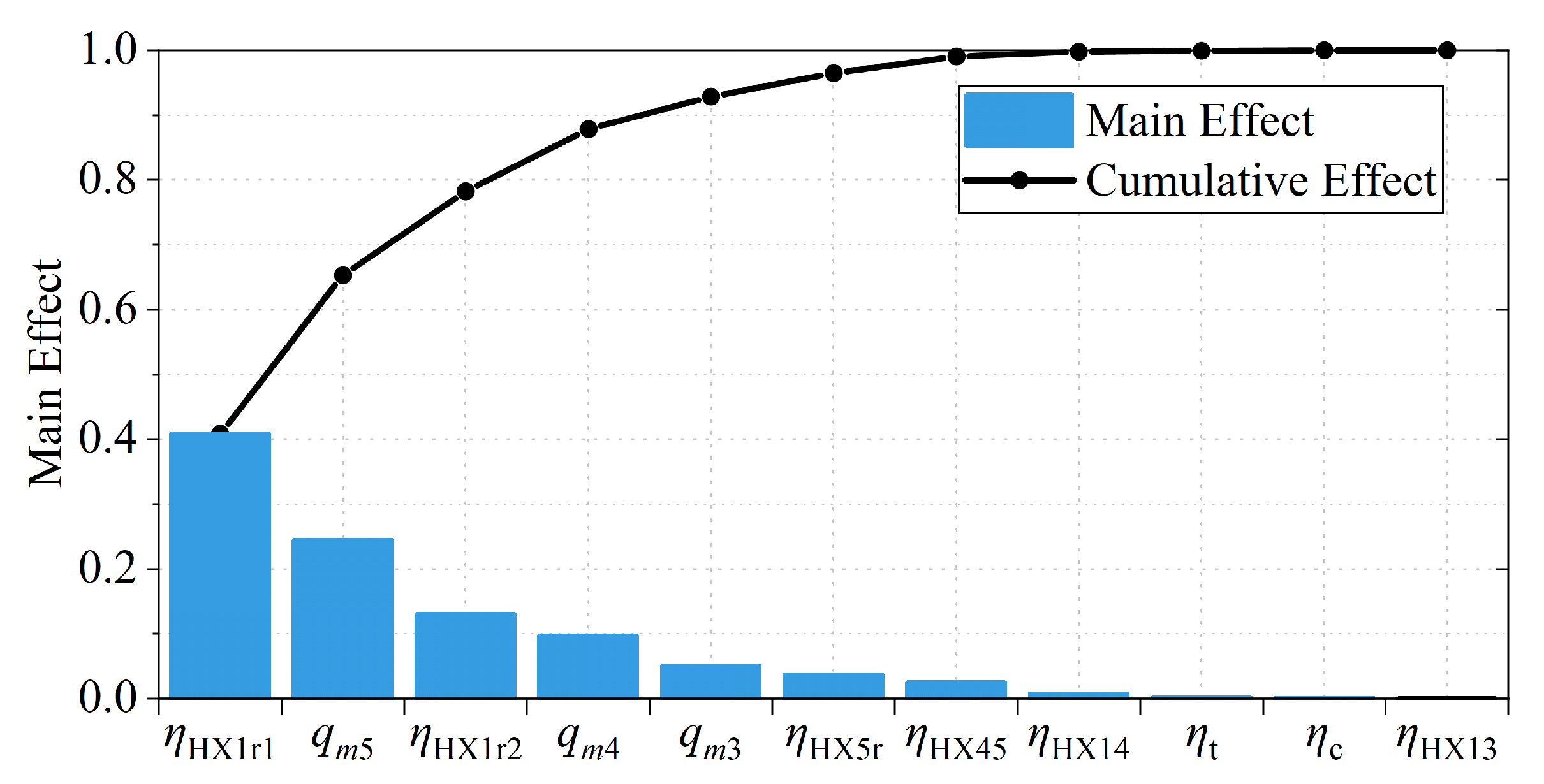
According to the parameter-matching calculation process and the thermal management system parameter-matching algorithm framework (Figure 3), the analysis of variance (ANOVA) was used to calculate the influence of the design variables on fuel consumption for the sensitivity analysis, as shown in Figure 7.

The results show that the ACS’s primary heat-exchanger efficiency, fuel-cycle flow rate, ACS’s secondary heat-exchanger efficiency, high-temperature liquid-cooling-cycle flow rate, low-temperature liquid-cooling-cycle flow rate and fuel/ram-air heat-exchanger efficiency had a greater impact on the fuel penalty. The total contribution rate of the parameters exceeds 0.95.

The heat exchangers contribute a large part of the system weight and their efficiency is important to the weight; thus, these parameters are more sensitive. Besides, since the mass flow rate of the subsystems is important to the heat flow of the heat exchangers, they also play a key role in weight calculation.

4. Optimal Design Calculation

4.1. Optimization Algorithm

Due to the high non-linearity of the parameter-matching calculations of the thermal management system, its fuel penalty value presents multi-peak or multi-valley characteristics. Therefore, the classical gradient-based optimization algorithm is easily affected by the initial value and falls into a local extreme point rather than the global optimal value. Under different initial conditions, based on the gradient-based method, there are large deviations during the optimization calculation process. In order to avoid the excessive influence of the initial value and make the optimization calculation results more accurate, this paper adopted the pattern search algorithm, genetic algorithm and particle swarm algorithm to optimize the design of the integrated thermal management system.

4.1.1. Pattern Search Algorithm

The calculation process of the pattern search algorithm is composed of two moving processes, namely, exploratory search and pattern move. Among them, the exploratory search is used to search for the general direction of the decline in the objective function to improve the accuracy of the search direction; the pattern move is to accelerate the movement according to the direction of the function change and find a better point [25]. The mathematical description of the searching process [26] is shown below.

For an n dimension function $f\left(\mathit{x}\right)$, set the initial point ${\mathit{x}}^{\left(0\right)}=\left(x_1^{\left(0\right)},x_2^{\left(0\right)},\cdots ,x_n^{\left(0\right)}\right)$, step size ${\alpha }_i>0$, base vector ${\mathit{e}}_i$ and the minimum calculation error $ϵ$. For the exploratory move, at the k-th step, ${\widehat{\mathit{x}}}^{(k,i)}$ means the point after i-th exploration; therefore,

$${\widehat{\mathit{x}}}^{(k,i)}=\left\{\begin{array}{cc}{\mathit{x}}^{\left(k\right)}\hfill & i=0\hfill \\ {\mathit{a}}^{(k,i)}={\widehat{\mathit{x}}}^{(k,i-1)}+{\alpha }_i{\mathit{e}}_i\hfill & f\left({\mathit{a}}^{(i,i)}\right)<f\left({\widehat{\mathit{x}}}^{(k,i-1)}\right)\hfill \\ {\mathit{b}}^{(k,i)}={\widehat{\mathit{x}}}^{(k,i-1)}-{\alpha }_i{\mathit{e}}_i\hfill & f\left({\mathit{a}}^{(i,i)}\right)<f\left({\widehat{\mathit{x}}}^{(k,i-1)}\right)\le f\left({\mathit{b}}^{(k,i)}\right)\hfill \\ {\widehat{\mathit{x}}}^{(k,i-1)}\hfill & \mathrm{otherwise}\hfill \end{array}\right.$$

(25)

After an exploratory move, if ${\widehat{\mathit{x}}}^{(k,n)}={\widehat{\mathit{x}}}^{(k,0)}$, the step size $\alpha$ should be reduced and the process repeated again until ${\widehat{\mathit{x}}}^{(k,n)}\ne {\widehat{\mathit{x}}}^{(k,0)}$ or $\alpha <ϵ$.

For the pattern move with step $\lambda$, the direction can be written as ${\mathit{D}}^{\left(k\right)}={\widehat{\mathit{x}}}^{(k,n)}-{\mathit{x}}^{\left(k\right)}$; then, the new point ${\widehat{\mathit{y}}}^{(k+1)}$ can be calculated as

$${\widehat{\mathit{y}}}^{(k+1)}={\widehat{\mathit{x}}}^{(k,n)}+\lambda {\mathit{D}}^{\left(k\right)}$$

(26)

If $f\left({\widehat{\mathit{y}}}^{(k+1)}\right)<f\left({\widehat{\mathit{x}}}^{(k,n)}\right)$, this round of iteration is finished and ${\mathit{x}}^{(k+1)}={\widehat{\mathit{y}}}^{(k+1)}$. Otherwise, the step size should be reduced and the process repeated.

By combining a series of exploratory searches and pattern moves, the algorithm can realize the optimization calculation of the objective function. The pattern search algorithm is relatively simple to implement and has high computational efficiency [27].

4.1.2. Genetic Algorithm

The genetic algorithm is a random search algorithm designed according to the natural selection and genetic mechanisms of the biological world.

Unlike traditional search algorithms, genetic algorithms start the search process from a set of randomly generated initial solutions, called a population. Each individual in the population is a solution, called a chromosome. These chromosomes evolve in subsequent iterations, called genetic. The algorithm optimizes the calculations by simulating the crossover, mutation and reproduction phenomena in natural selection and genetic process [28].

Crossover or mutation operations generate the next generation of chromosomes, called progeny. The goodness of chromosomes is measured by fitness. A certain number of individuals are selected from the previous generation and the offspring according to the fitness, as the next generation population; then, the evolution continues. After several generations, the algorithm converges on the best chromosome, which is likely to be the optimal solution.

The concept of fitness is used in the genetic algorithm to measure the degree to which each individual in the population is likely to reach the optimal solution in the optimization computation. The definition of the fitness function is generally related to the specific solution problem.

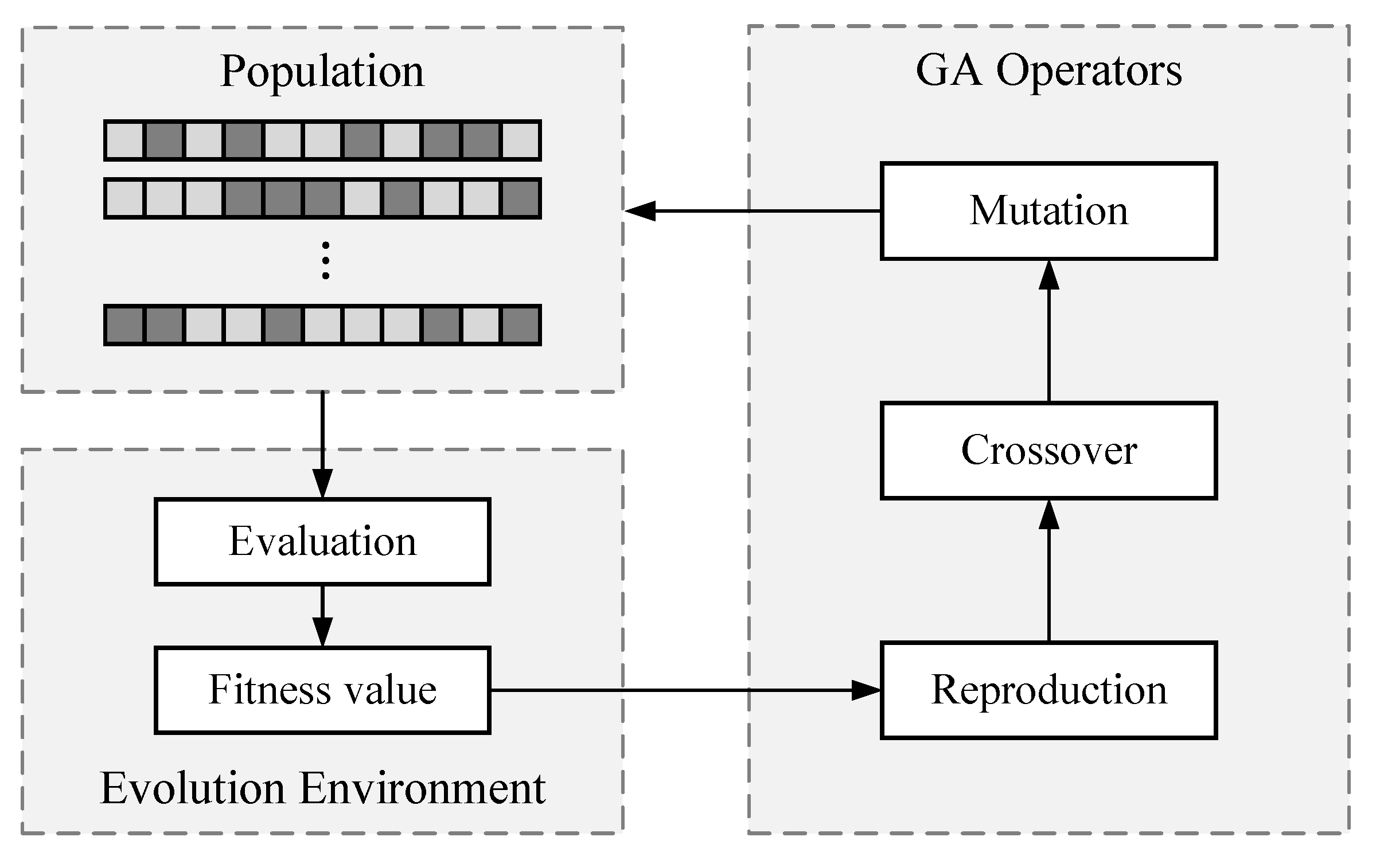
In each round of calculations, a set of candidate solutions are retained; then, better individuals are selected from them and these individuals are combined using operations to form a new generation of candidate program groups. The above process has to be repeated until the convergence condition of the solution is met. The genetic algorithm can realize distributed information collection and exploration in the entire solution space and can avoid the solution process falling into the local extreme point. The flow diagram of the genetic algorithm [29] is shown in Figure 8.

4.1.3. Particle Swarm Algorithm

The particle swarm algorithm is a kind of random algorithm that simulates the group behavior of flocks or groups of fish in nature. These populations adopt a cooperative mode when searching for food and each particle (individual) adjusts its search strategy according to its own and surrounding experience [30], so that the entire population can reach the goal faster.

The algorithm is population-based and moves individuals to better regions based on their fitness to the environment. However, instead of using evolutionary operators for individuals, it treats each individual as a volumeless particle (point) in a N-dimensional search space, flying at a certain speed in the search space, which is dynamically adjusted according to its own flight experience and the flight experience of its peers. The i-th particle is denoted as $X_i=\left(x_{i1},x_{i2},\cdots ,x_{iN}\right)$ and the best position it has experienced (with the best adaptation value) is denoted as $P_i=\left(p_{i1},p_{i2},\cdots ,p_{iN}\right)$, also known as pbest. The index number of the best position experienced by all particles in the population is denoted by the symbol g, i.e., $P_g$, also known as gbest. The velocity of particle i is denoted by $V_i=\left(v_{i1},v_{i2},\cdots ,v_{iN}\right)$. For each generation, its $(n+1)$-st dimension $(1\le n+1\le N)$ varies according to the following equation:

$$\begin{array}{c}{v}_{i,n+1}=w·v_{i,n}+c_1·\mathrm{rand}\left(\right)·(p_{i,n}-x_{i,n})+c_2·\mathrm{rand}\left(\right)·(p_{g,n}-x_{i,n})\end{array}$$

(27)

$$\begin{array}{c}{x}_{i,n+1}=x_{i,n}+v_{i,n+1}\end{array}$$

(28)

where w is the inertia weight, $c_1$ and $c_2$ are acceleration constants and rand() generates random values varying in the range $[0,1]$.

In addition, the velocity $V_i$ of the particle is limited by a maximum velocity $V_{max}$. If the current acceleration of the particle causes its velocity $v_{i,n}$ in a dimension to exceed the maximum velocity $v_{max,n}$, the velocity is limited to it.

In Equation (27), the first part is the inertia of the particle’s previous behavior; the second part is the “cognition” part, which represents the thinking of the particle itself; and the third part is the “social” part, which represents the information sharing and mutual cooperation between the particles.

The particle swarm algorithm uses the following psychological assumption: In the process of seeking consistent cognition, individuals tend to remember their own beliefs and consider the beliefs of their colleagues at the same time. When they perceive that their colleagues’ beliefs are better, they adapt.

The algorithmic process of the standard particle swarm algorithm is shown as follows:

• Initialize a group of particles (population size, m), including random positions and velocities;
• Evaluate the fitness of each particle;
• For each particle, compare its adaptation value with that of the best position pbest it has experienced and, if it is better, use it as the current best position pbest;
• For each particle, compare its adaptation value with that of the best position gbest experienced globally and reset the index number of gbest if it is better;
• Vary the velocity and position of the particles according to Equations (27) and (28);
• If the end condition is not reached (usually a sufficiently good adaptation value or reaching a preset maximum algebra $G_{max}$), return to step 2.

4.2. Selection of Optimal Variables

The variables were chosen to optimize the value of fuel penalty, which is based on the parameter-matching calculation of the thermal management system. The ranges of the variables are shown in

Table 3. Ranges of thermal management system optimization variables.

Variables	Name	Min	Max
${\eta }_{HX1r1}$	Efficiency of ACS’s primary HX	0.45	0.9
${\eta }_{HX1r2}$	Efficiency of ACS’s secondary HX	0.45	0.9
${\eta }_{HX13}$	Efficiency of air/low-temperature liquid-cooling HX	0.45	0.85
${\eta }_{HX14}$	Efficiency of air/high-temperature liquid-cooling HX	0.45	0.85
${\eta }_{HX45}$	Efficiency of fuel/high-temperature liquid-cooling HX	0.45	0.85
${\eta }_{HX5r}$	Efficiency of fuel/ram-air HX	0.45	0.85
${\eta }_c$	Efficiency of ACS’s compressor	0.6	0.8
${\eta }_t$	Efficiency of ACS’s turbine	0.6	0.8
$q_{m3}$	Flow rate of low-temperature liquid-cooling cycle	0.6	2.5
$q_{m4}$	Flow rate of high-temperature liquid-cooling cycle	0.6	2.5
$q_{m5}$	Flow rate of fuel cycle	0.6	2.5

.

The optimization was performed twice within the scope of the design, as follows:

• All 11 design variables were taken as optimized design variables to perform optimization calculations;
• According to the calculation results of the sensitivity analysis, six variables, i.e., (1) efficiency of ACS’s primary HX, (2) flow rate of fuel cycle, (3) efficiency of ACS’s secondary HX, (4) flow rate of high-temperature liquid-cooling cycle, (5) flow rate of low-temperature liquid-cooling cycle and (6) efficiency of fuel/ram-air HX, affected the fuel penalty significantly. Therefore, these variables were set as optimization design variables to perform optimization calculations. The remaining five variables were set as constants.

4.3. Optimization Calculation Results

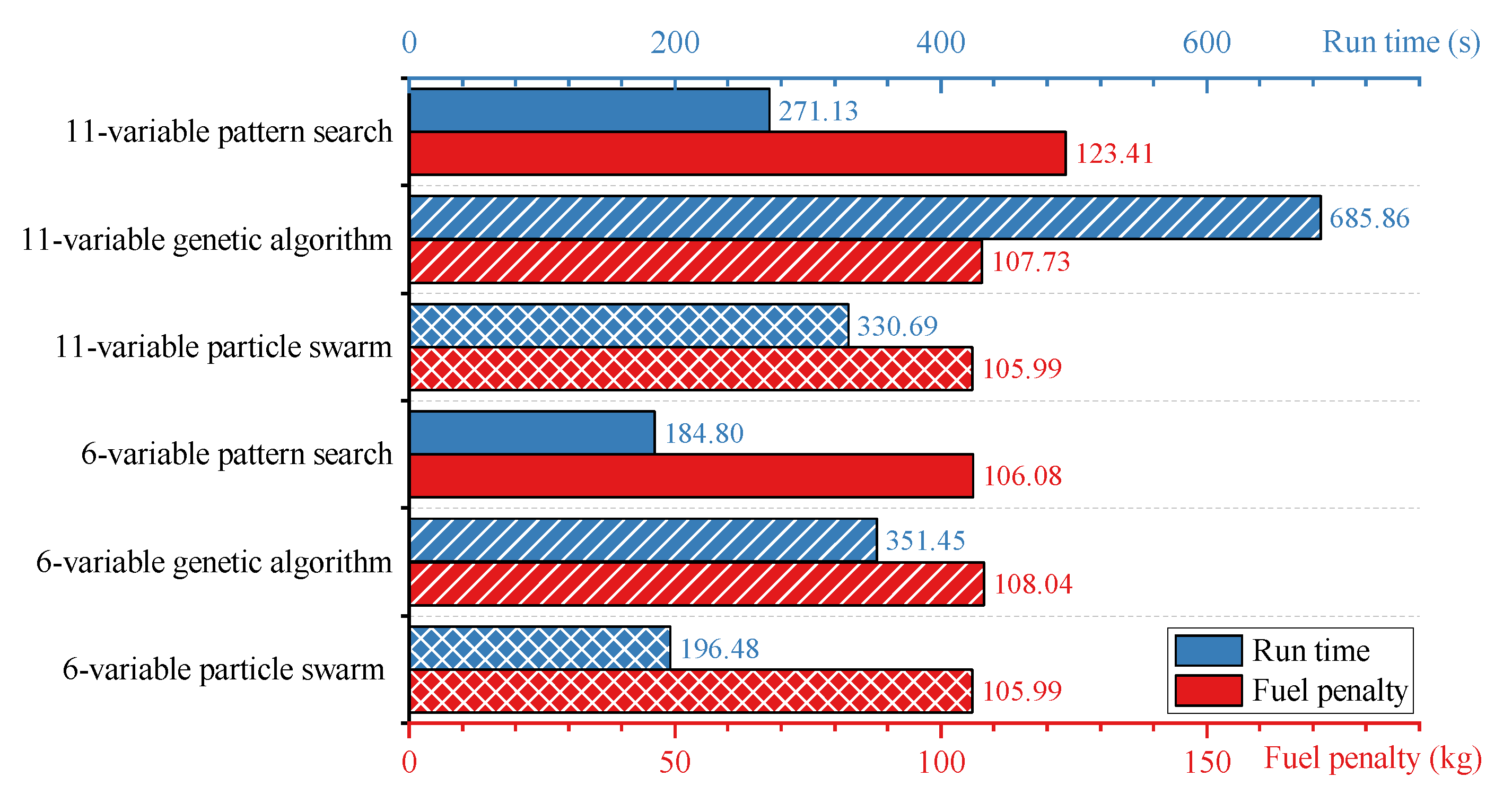
Using the global optimization toolbox in MATLAB, we developed the code for the optimization algorithms. According to the maximum and minimum values of each variable defined in Table 3, pattern search, genetic algorithm and particle swarm algorithm were used to optimize the 11-variable scheme and the simplified 6-variable scheme. The ground conditions were chosen as the design conditions. The initial optimization variables and the optimization results obtained by the three optimization algorithms are summarized in

Table 4. Comparison of two optimization designs’ results of the integrated thermal management system.

Variables	11 Variables			6 Variables
	Search	GA	Particle	Search	GA	Particle
${\eta }_{HX1r1}$	0.6137	0.5329	0.5372	0.5498	0.5370	0.5372
$q_{m5}$	0.6215	0.6089	0.6009	0.6068	0.6057	0.6013
${\eta }_{HX1r2}$	0.7992	0.7240	0.7287	0.7122	0.7286	0.7294
$q_{m3}$	1.8873	0.7252	0.7018	0.7191	0.7023	0.6998
$q_{m4}$	0.6769	0.6001	0.6000	0.6000	0.6000	0.6000
${\eta }_{HX5r}$	0.7254	0.6203	0.6170	0.6212	0.6173	0.6170
${\eta }_{HX45}$	0.5542	0.4974	0.4954	0.5 (fixed)	0.5 (fixed)	0.5 (fixed)
${\eta }_{HX14}$	0.4500	0.4504	0.4500	0.45 (fixed)	0.45 (fixed)	0.45 (fixed)
${\eta }_t$	0.8000	0.8000	0.8000	0.8 (fixed)	0.8 (fixed)	0.8 (fixed)
${\eta }_c$	0.7505	0.8000	0.8000	0.8 (fixed)	0.8 (fixed)	0.8 (fixed)
${\eta }_{HX13}$	0.5997	0.4505	0.4500	0.45 (fixed)	0.45 (fixed)	0.45 (fixed)
$m_f$	123.4105	107.7315	105.9917	106.0776	108.0401	105.9921

Search, pattern search algorithm; GA, genetic algorithm; Particle, particle swarm algorithm.

. The optimization results and calculation time for different variables and optimization algorithms are shown in Figure 9. The 6-variable optimization calculations consumed less time than those of the 11-variable optimization. Except for the 11-variable pattern search algorithm, the optimized fuel penalty results are not significantly different.

4.4. Discussion

The particle swarm algorithm and genetic algorithm are intelligent optimization algorithms, which avoid the multi-peak or valley phenomena of the objective function. They performed well and could find the global optimal value. The results show that the difference between the minimum fuel penalty is small. Furthermore, the results of the optimized variables are relatively close.

Pattern search is an improved gradient-based optimization algorithm. The algorithm overcame the shortcomings of traditional optimization algorithms to a large extent, which performed well in the optimization process of 6 variables. Besides, the algorithm basically achieved the global optimal results. However, during the process of optimizing 11 variables, the variables still fell into a local minimum, where no global optimal solutions were found. Therefore, in the case where the number of variables was higher, there were still certain limitations related to the pattern search optimization algorithm.

The calculation results of the 6 optimized variables selected by the variable sensitivity analysis are generally close to the calculation results of all 11 variables. Besides, the drop in the number of variables greatly reduced the calculation time.

In general, the pattern search algorithm obtained better results with the least run time in the six-variable calculations. Although the particle swarm algorithm took a longer time, it performed well in the optimization calculation process of both the 11 variables and 6 variables. Additionally, the optimal value of each variable could be obtained during the process. Among the three optimization algorithms, the genetic algorithm took the longest time.

Therefore, it is recommended to comprehensively consider the trade-off of consumed time and calculation accuracy when optimizing the integrated thermal management system. The six-variable pattern search or particle swarm optimization algorithm is the first choice.

5. Conclusions

This paper studies the integrated thermal management system. We developed a whole process for optimizing the system, including the hierarchical parameter-matching algorithm, the sensitivity analysis of the system parameters and optimization design calculations. The main conclusions are reported below.

• The composition characteristics of the integrated thermal management system were analyzed in depth. Based on the analysis, a four-level parameter-matching calculation method of system, subsystems, components and thermodynamic properties was designed.
• The parameter sensitivity analysis was conducted based on parameter-matching calculations. Through the parameter-matching process and system thermodynamic analysis, 11 design variables were initially selected. The 11 design variables were reduced to 6 variables by the sensitivity analysis. The six variables are (1) efficiency of ACS’s primary HX, (2) flow rate of fuel cycle, (3) efficiency of ACS’s secondary HX, (4) flow rate of high-temperature liquid-cooling cycle, (5) flow rate of low-temperature liquid-cooling cycle and (6) efficiency of fuel/ram-air HX.
• The optimization of the integrated thermal management system is complicated because of the multi-extremum problem. The variables optimized by traditional gradient-based optimization algorithms easily fall into the local extremum point. Therefore, the pattern search, genetic algorithm and particle swarm algorithm were selected for optimization calculation and comparative analyses. The results show that the particle swarm optimization and genetic algorithm could find the global optimal value more easily. Among them, the particle swarm algorithm took the lowest amount of time.
• The algorithm in this paper is mainly aimed at the structural design of the integrated thermal management system of aircrafts. However, it could also be applied to other fields. For thermal systems with similar hierarchical structures, the same idea can be used for parameter matching, sensitivity analyses and optimization design calculations.