Article

Mixed-Sensitivity Control for Drag-Free Spacecraft Based on State Space

1
School of Aeronautics and Astronautics, Sun Yat-sen University, Shenzhen 528406, China
2
School of Physics and Astronomy, Sun Yat-sen University, Zhuhai 528478, China
*
Author to whom correspondence should be addressed.
These authors contributed equally to this work.
Aerospace 2022, 9(11), 708; https://doi.org/10.3390/aerospace9110708
Submission received: 28 August 2022 / Revised: 28 October 2022 / Accepted: 7 November 2022 / Published: 12 November 2022
(This article belongs to the Special Issue Emerging Space Missions and Technologies)

Abstract

:
This paper investigates a mixed-sensitivity control method for a class of drag-free spacecraft-needed frequency-separation control, which overcomes the coupled problem of a multiple-in multiple-out (MIMO) system with multiple sensitive-axes and disturbances of actuators. Firstly, the relative dynamics equation is established based on the character of displacement error, which is separated by that test-mass (TMs) tracking ideal orbit with high-frequency displacement and cavity of spacecraft tracking TMs with low-frequency displacement. Secondly, the feedback gain matrix is obtained by the LMI/SDP, which is devised by a general system containing a weight function. Finally, the simulation results demonstrate the performance of the proposed method.

1. Introduction

In recent years, drag-free spacecraft has been applied in an increasing number of fields, and an incrementally increasing number of researchers have been attracted to carrying out this work, thanks to the project Observations of the Earth’s Gravity (OEG) [1,2,3], the Verification of Basic Theory (VBT) [4,5,6], and the Detection of Gravitational Wave (DGW) [7,8,9]. The concept of drag-free was first introduced by Lange B in the 1960s [10]; then, it was realized on TRIAD I, which was used to improve the precision of orbit determination [11]. GOCE was a gravitational satellite lunched after CHAMP and GRACE; its technology of drag-free has been quite sophisticated, which can precisely measure data of the earth’s gravitational field [2]. GP-B was a satellite for verifying general relativity, which has made the acceleration below 10 9   m s 2 Hz 1 / 2 in the sensitive axis [4]. Projects of DGW represented by LISA [12], Taiji [13], and TianQin [9] also demand high performance. The issue of drag-free could continue to be studied in the future.
Many scholars have done valuable research in the area of control for drag-free, such as PID [14], LQR [15], embedded model control (EMC) [16], H [17], sliding model control (SMC) [18,19], and adaptive control [20]. In order to obtain the estimated state of a drag-free system that has complex parameter structures, a controller with a high-gain observer was designed [21]. A LQR control based on modern optimal control theory was used to solve drag-free and attitude control with cold interferometry [22]. For uncertain disturb, an EMC [23] and an self-recurrent wavelet neural network disturbance observer [24] were designed to estimate it and a SMC [18] was proposed to overcome it. There was a robust predictive control (MPC) to constraint test-mass moving in the cavity [25]. For variation of space parameters, an adaptive method was proposed to meet drag-free control [26]. These studies have addressed both general and specific problems.
In order to establish that the signal of drag-free control is mixed in the scientific signal in DGW, a mixed-sensitivity controller was designed to separate frequency-bands [27]. However, it only has robustness for parameter perturbation instead of robust stability for disturbance and noise. To solve this problem, this paper designs a new mixed-sensitivity mentioned in reference [28,29] that is based on state space. Compared with output feedback in the frequency domain, state feedback in the time domain is more mature for the attached observer, the extended observer, and so on. Moreover, there is no need for decoupling.
To sum up, the control system of drag-free has achieved great things in the field of theory and projects. This paper is built on previous designs of a mixed-sensitivity controller based on state space that has robust stability against disturbance and noise and is available for the MIMO system. The contribution of this paper is that a generalized system based on state space is obtained by combining a drag-free system model based on a relative dynamics equation and a filter based on a weight transfer function, and a state feedback matrix ensuring closed-loop system is stable is obtained through Lyapunov’s second theory.

2. Model Building

Drag-free spacecraft has the test mass for scientific detection and the satellite body for offsetting disturbance. Traditional drag-free spacecraft with single TMs places the test mass on the ideal orbit and traces it depending on the spacecraft body.

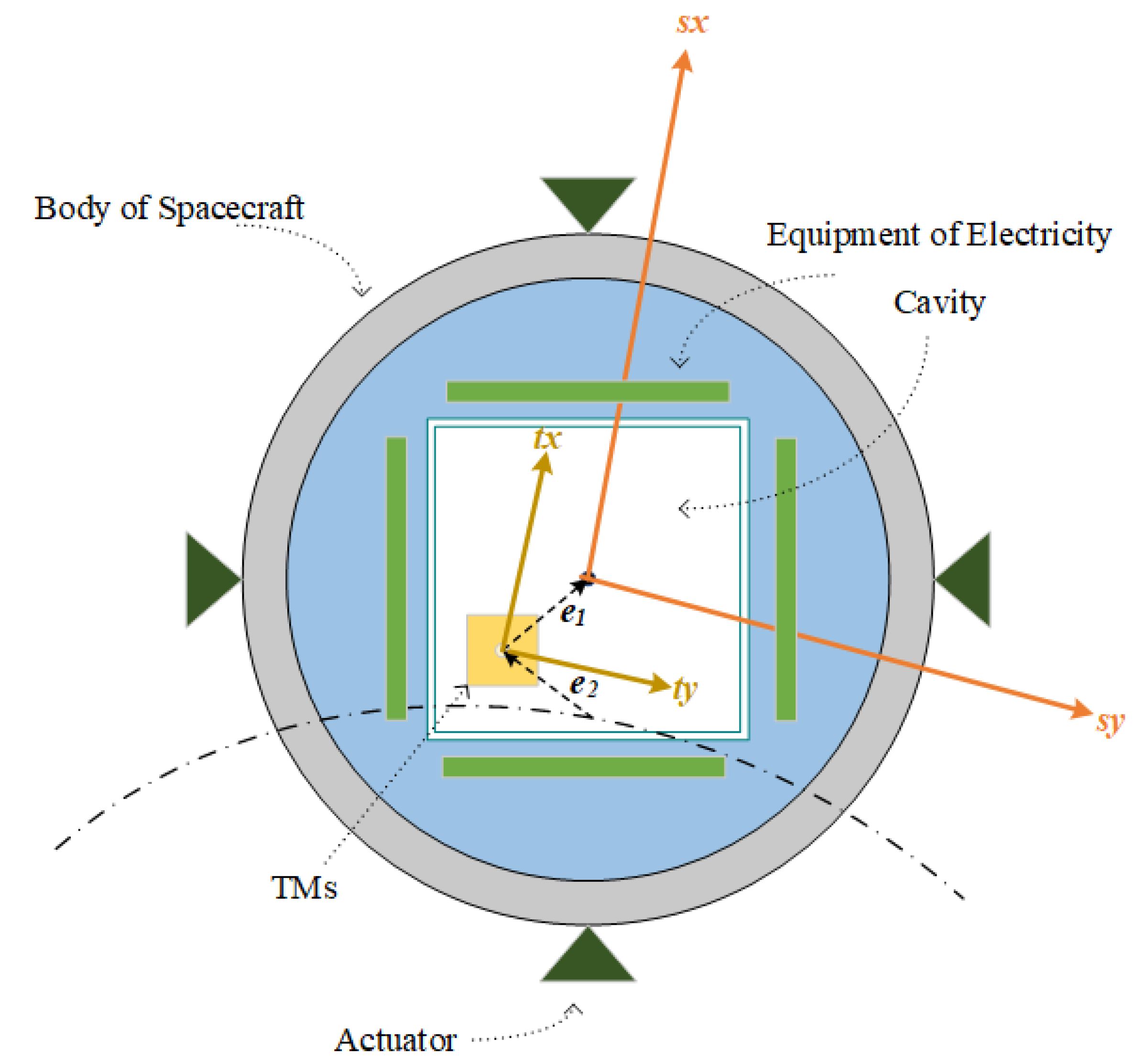
2.1. Reference Coordinate System

In order to establish a relative dynamics equation for the body of spacecraft and the TMs. There are four reference coordinate systems that have to be defined at least. The reference frames are shown in Figure 1 and are
  • The earth inertial reference coordinate system (IRS): The origin of coordinates is located at the center of the earth. ix-axis points to the vernal equinox, and the iz-axis is directed toward the n-pole. The iy-axis follows the right-handed rule.
  • The ideal orbit reference coordinate system (ORS): The origin of the coordinates is located at the ideal orbit. The ix-axis points to the opposite direction of the center of the earth. The iy-axis coincides with the velocity vector direction of the spacecraft. They are located in the orbital plane. The iz-axis follows the right-handed rule.
  • The spacecraft body reference coordinate system (SRS): The coordinate axes are parallel to the ORS, but the origin of the coordinates is located at the center of the cavity.
  • The TMs reference coordinate system (TRS): The coordinate axes are parallel to the ORS, but the origin of the coordinates is located at the mass center of the TMs.

2.2. Problem Modeling

The traditional gravity field determination uses two different control types.
(1)
The mode of displacement: The relative displacement is measured directly, and the signal is transferred to the control system of drag-free in order to offset disturbance.
(2)
The mode of accelerometer: The displacement due to disturbance is offset by the control system of electrostatic suspension; then, the control system of drag-free adjusts the body position according to the reaction force.
Now, let us consider gravitational wave detection. Because of the satellite formation dimension, it has a problem measuring the frequency band. The signal of the gravitational wave is only available in a certain frequency band instead of all frequency bands. In order to avoid mixing the control signal into the gravitational wave signal, which makes data processing more difficult, a frequency-separation idea was adopted. Only one threshold value can exist for a mixed-sensitivity controller, so there are two designed controllers for the control systems of drag-free and electrostatic suspension, respectively.The main disturbances received by drag-free spacecraft in space are solar radiation pressure, which acts on the outer loop at low frequency, and electrostatic force, which acts on the inner loop at high frequency. In summary, it is obvious to offset the low-frequency disturbance with mode 1 and offset the high-frequency one with mode 2.
There are three different displacement errors in Figure 2:
e 1 = r 1 r l e 2 = r 2 r h e 3 = r g w
where e 1 and r l are the relative position vector from TMs to the center of the cavity in the TRS and displacement by low-frequency disturbance, respectively; e 2 and r h are the relative position vector from ideal orbit to TMs in the ORS and displacement by high-frequency disturbance, respectively; r 1 and r 2 are outputs of displacement; and r g w is gravitational wave signal.

2.3. Dynamics Modeling

The consideration of the two-body equation is as follows:
d 2 r s d t 2 = μ r s r s 3 + u s + d s
d 2 r t d t 2 = μ r t r t 3
d 2 r t d t 2 = μ r t r t 3 + u t + d t
d 2 r o d t 2 = μ r o r o 3
where r s represents the distance between the center of the cavity of the spacecraft and the earth in the IRF components; r t represents the distance between the center of mass of the TMs and the earth in the IRF components; and r o represents the distance between the ideal orbit and the earth in the IRF. u s and u t are the control force, which is comprised of cold air thrust and electrostatic suspension force, respectively. d s and d t are the disturbing force, which is comprised of the noise of the actuator and static.
Let (2) minus (3), (4) minus (5), to obtain the relative dynamics equation and transform it into the CW equation as follows:
r ¨ 1 = 2 ω × r ˙ 1 ω × ( ω × r 1 ) ω ˙ × r 1 + μ r t r t 3 r s r s 3 + u s + d s
r ¨ 2 = 2 ω × r ˙ 2 ω × ( ω × r 2 ) ω ˙ × r 2 + μ r o r o 3 r t r t 3 + u t + d t
where ω is the spacecraft or TMs angular velocity in the IRS, which is orbit angular velocity.
Since there is a coupling problem between the z-axis and the orbital angular velocity vector in the CW equation, the z-axis is discarded. Note that the two-TMs drag-free spacecrafts used in gravitational wave detection also have two sensitive axes in the orbital plane and that frequency-separation is the most promising for gravitational wave detection. Hence, it was practically meaningful to discard the z-axis. Equations (6) and (7) are transformed into the form of the linear equation of the matrix as follows:
x ¨ 1 y ¨ 1 = 2 0 ω ω 0 x ˙ 1 y ˙ 1 0 ω ω 0 y 1 ω x 1 ω 0 ω ˙ ω ˙ 0 x 1 y 1 + μ r t 3 x 1 y 1 + u s + d s
x ¨ 2 y ¨ 2 = 2 0 ω ω 0 x ˙ 2 y ˙ 2 0 ω ω 0 y 2 ω x 2 ω 0 ω ˙ ω ˙ 0 x 2 y 2 + μ r o 3 x 2 y 2 + u t + d t
Select state variables X 1 = [ x 1 , x ˙ 1 , y 1 , y ˙ 1 ] T and X 2 = [ x 2 , x ˙ 2 , y 2 , y ˙ 2 ] T . Equations (8) and (9) are transformed into the form of equation of state as follows:
X ˙ 1 = A 1 X 1 + B 1 U s + B 1 d s Y 1 = C 1 X 1
where
A 1 = 0 0 1 0 0 0 0 1 ω 2 μ r t 3 ω ˙ 0 2 ω ω ˙ ω 2 μ r t 3 2 ω 0
B 1 = 0 0 0 0 1 0 0 1 , C 1 = 1 0 0 0 0 1 0 0
X ˙ 2 = A 2 X 2 + B 2 U t + B 2 d t Y 2 = C 2 X 2
where
A 2 = 0 0 1 0 0 0 0 1 ω 2 μ r o 3 ω ˙ 0 2 ω ω ˙ ω 2 μ r o 3 2 ω 0
B 2 = 0 0 0 0 1 0 0 1 , C 2 = 1 0 0 0 0 1 0 0
The above comprises the relative dynamics equation of the drag-free system and the electrostatic suspension system. The controller designed by two equations was used in different frequencies.

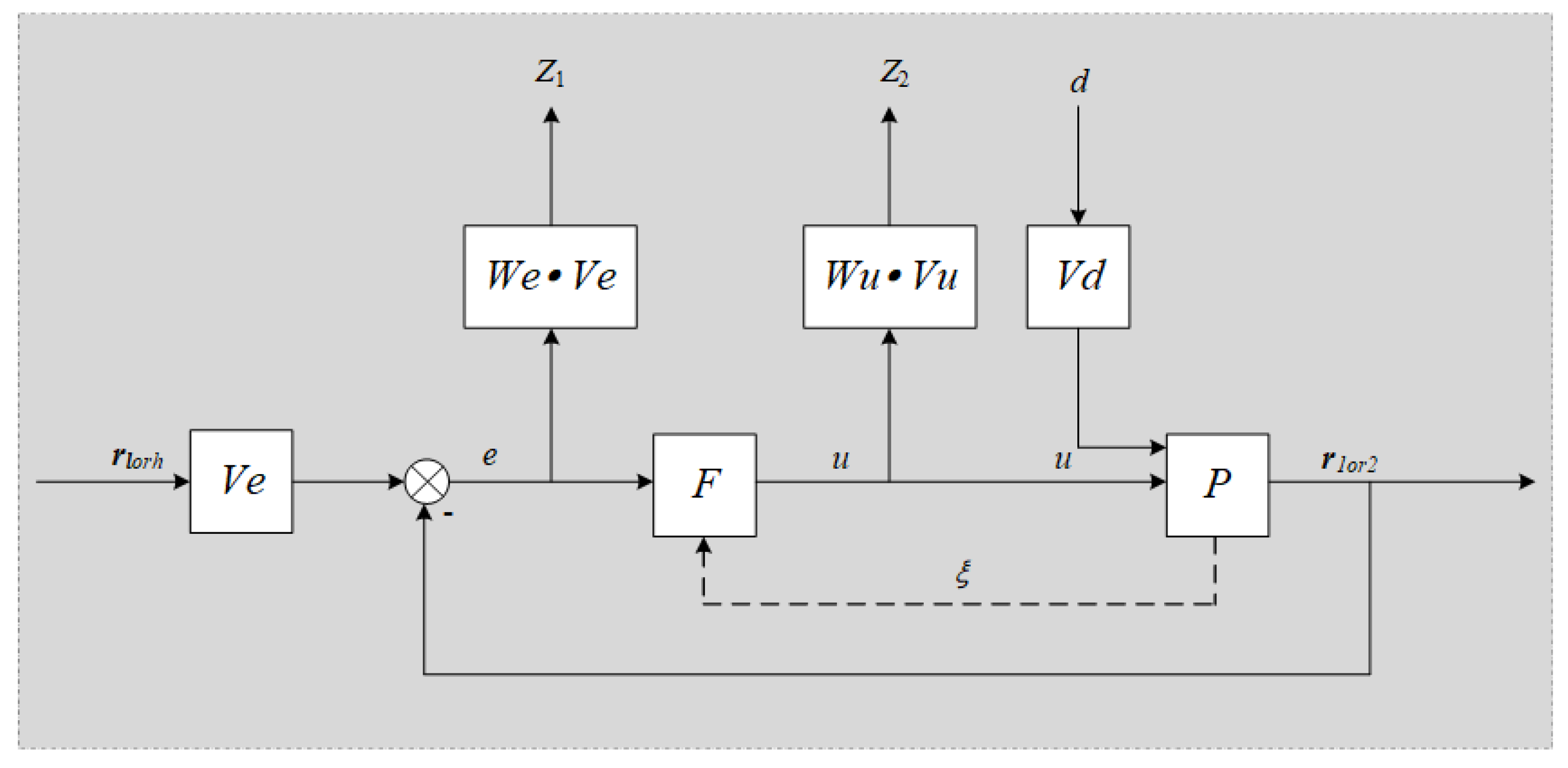
3. Controllers Designing

Theorem 1 
([30]). For a system P
ξ ˙ = A ξ + B 1 ζ 1 + B 2 ζ 2 Y = C ξ
and a general system G about P
ξ ˙ = A ξ + B 1 ζ 1 + B 2 ζ 2 Z 1 = C 1 ξ + D 1 ζ 1 Z 2 = C 2 ξ + D 2 ζ 2 Y = C ξ
There ia a state feedback matrix K that is designed as the control law ζ 2 = K ξ such that | p ( G , K ) | < γ if there is a symmetric position definite matrix Y
Y A ^ T + A ^ Y γ B 2 T Y C 1 T B 1 * γ I D 1 * * γ I < 0
where A ^ = A C 2 B 2 ; moreover, the K is designed as K = ( γ B 2 T Y 1 + C 2 )
Proof. 
Only stability is demonstrated here. For system (13), select the Lyapunov function as
V = ξ T Y ξ > 0
then
V ˙ = ξ ˙ T Y ξ + ξ T Y ξ ˙ = ( A ξ + B 1 ζ 1 + B 2 ζ 2 ) T Y ξ + ξ T Y ( A ξ + B 1 ζ 1 + B 2 ζ 2 ) = ξ T ( A T Y + YA + B 2 T K T Y + YK B 2 ) ξ + ζ 1 T B 1 T Y ξ + ξ T Y B 1 ζ ξ T ( A T Y + YA + B 2 T K T Y + YK B 2 + Y B 1 B 1 T ) ξ + ζ 1 T ζ 1 ξ T ( A T Y + YA + B 2 T K T Y + YK B 2 + YB B 1 T Y + γ 1 C 1 T C 1 ) ξ + D 1 D 1 = ξ T ( A T Y + YA + B 2 T ( γ B 2 T Y 1 + C 2 ) T Y + Y ( γ B 2 T Y 1 + C 2 ) B 2 + B 1 T Y + γ 1 C 1 T C 1 ) ξ + D 1 D = ξ ( A ^ Y + Y A ^ γ B 2 B 2 T + B 1 T Y + γ 1 C 1 T C 1 ) ξ + D 1 D 1 < 0
then the above equation is multiplied by Y and Y 1 simultaneously and replaced Y 1 with Y . According to Schur complement, (14) was gained. □

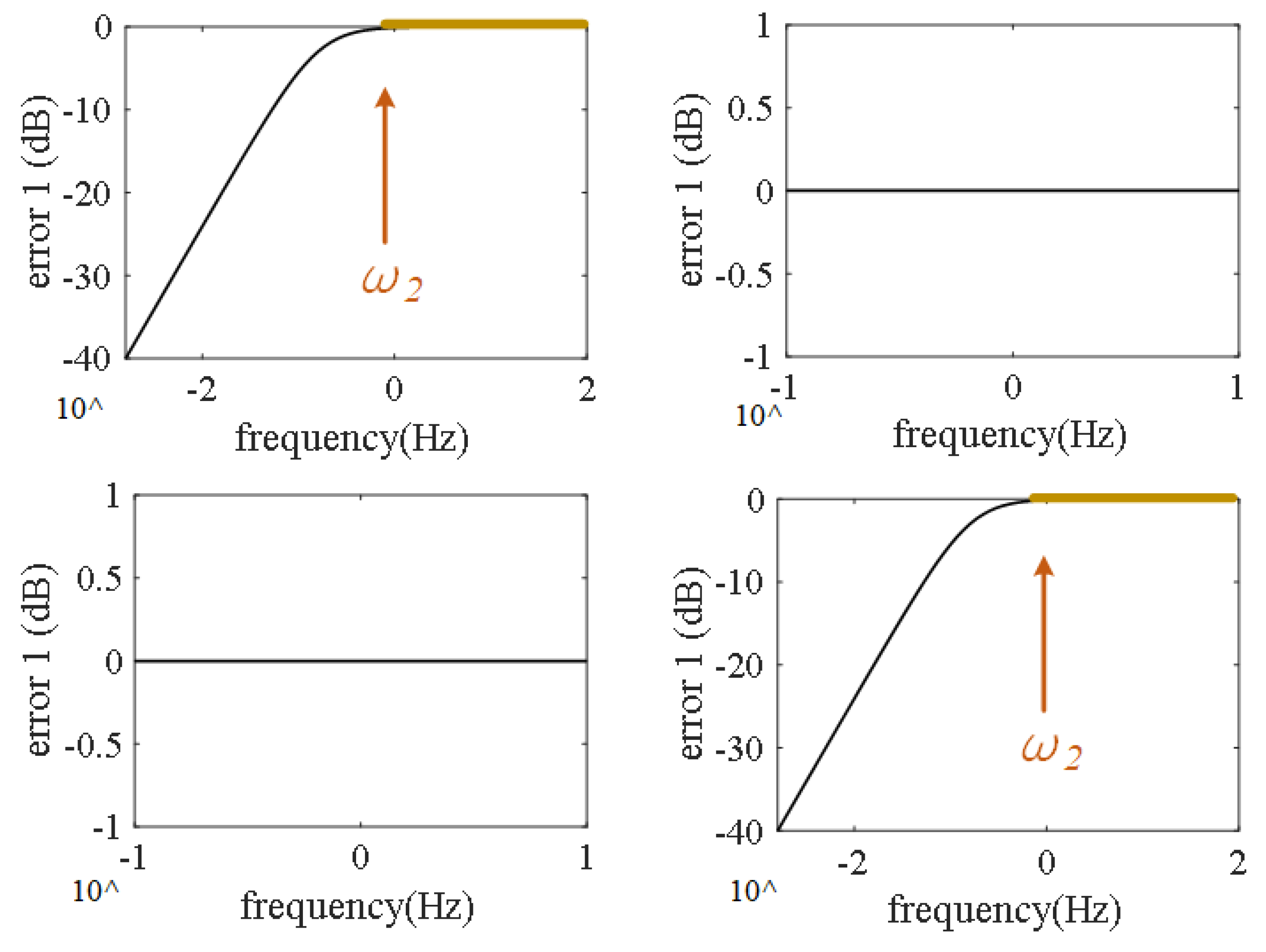
3.1. Weight Selection

This subsection discusses a weight-transfer function. The gravitational wave source is in a specific frequency band that is from ω 1 to ω 2 . According to Section 2.2, there is a spacecraft controller for ω 1 or less and a TMs controller for ω 2 or the above. For each engineering of gravitational wave detection, the frequency band of the wave source is different. This paper adopted TianQin engineering with f ( ω 1 = 10 4 Hz , ω 2 = 1 Hz ) .
A simple mixed-sensitivity controller for a closed-loop system is shown in Figure 3. The weighting filter We is used to adjust the steady-state error between the input and the output, which is also called the shape of sensitivity. The requirements for selecting We are large steady-state errors when in the tracking band and small ones when in the non-tracking band. To reach the requirement, select the following transfer function:
We = ω s + a ω 1 s + 1 0 0 ω s + a ω 1 s + 1
where ω is ω 1 or ω 2 , and a is a constant. For the system of multiple-input and multiple-output, it is an n-order matrix. Since the sensitivities of the x-axis and y-axis are identical, the elements of We are uniform. They can be different if their sensitivities are different.
The weighting filter Wu is used to adjust the shape of the control sensitivity and to represent actuator limitations and robustness. The requirement for selecting Wu is matching it to the We, which makes LMI available. The specific requirement is available from reference [31]. To reach the requirement, select the following transfer function:
Wu = ω 1 s + a ω s + 1 0 0 ω 1 s + a ω s + 1
Substitute ω 1 to (17) and (18). The real weighting filter for the control system of drag-free is as follows:
W e 1 = 10 4 s + 1 10 4 s + 1 0 0 10 4 s + 1 10 4 s + 1 W u 1 = 10 3 s + 1 10 4 s + 1 0 0 10 3 s + 1 10 4 s + 1
As in Figure 4, when the frequency is above 10 4 Hz, the magnitude response declines gradually. It represents the fact that We has a simple filtering effect that separates frequency at 10 4 Hz.
Substitute ω 2 to (17) and (18). The real weighting filter for the control system of electrostatic suspension is as follows:
W e 2 = s s + 1 0 0 s s + 1 W u 2 = 10 1 s + 1 s + 1 0 0 10 1 s + 1 s + 1
As in Figure 5, when the frequency is below 1 Hz, the magnitude response declines gradually. It represents the fact that We has a simple filtering effect that separates the frequency at 1 Hz.
We does not determine the sensitivity of the closed-loop system, but its filtering effect is the same with the closed-loop system. Specific parameters can be chosen in the experiment.

3.2. Gain Matrix

As Figure 3, e is the error between disturb input and metrical output. u is the control signal. V e is the coefficient of e representing the ideal upper limit. V u has the same function for u . To meet the form in reference [28], construct two new variables as follows:
e ^ = e + CX u ^ = D W u V u 1 u

3.2.1. Drag-Free

Considering (13), Z 1 and Z 2 are controlled outputs; they can be replaced by We and Wu, which impact the sensitivity of the closed-loop system. The new general system is shown in Figure 3. In order to solve LMI in the time domain, translate (19) into an equation of state. As follows:
X We 1 = A We 1 X We 1 + B We 1 e Y We 1 = C We 1 X We 1 + D We 1 e
where
A We 1 = 10 4 0 0 10 4 , B We 1 = 1 0 0 1 C We 1 = 10 4 0 0 10 4 , D We 1 = 10 8 0 0 10 8 and
X Wu 1 = A Wu 1 X Wu 1 + B Wu 1 u Y Wu 1 = C Wu 1 X Wu 1 + D Wu 1 u
where
A Wu 1 = 10 4 0 0 10 4 , B Wu 1 = 1 0 0 1 C Wu 1 = 10 11 0 0 10 11 , D Wu 1 = 10 7 0 0 10 7
Regarding system (10), it is a real system. To meet the frequency-separation of the drag-free control signal, set the general system S 1 based on the state space. The state variables of X 1 and X W e 1 , X W u 1 are the set general state variable X S 1 = [ X 1 T , X W e 1 T , X W u 1 T ] T , which meet the general system requirement. Then, the general system S 1 is as follows:
X ˙ S 1 = A S 1 X S 1 + B S 11 e ^ + B S 12 u ^ Y S 11 = C S 11 X S 1 + D S 11 e ^ Y S 12 = C S 12 X S 1 + D S 12 u ^
where
A S 1 = A 1 0 0 B W e 1 V e 1 C 1 A W e 1 0 0 0 A W u 1 B S 11 = 0 B W e 1 0 , B S 12 = B 1 V u D W u 1 1 0 B W u 1 D W u 1 1 C S 11 = 0 C W e 1 0 , C S 12 = 0 0 C W u 1 D S 11 = D W e 1 , D S 12 = I
Considering (14) and (28), the gain matrix K 1 of the general system (28) can be solve by LMI (14). To have the optimal solution of γ , try to solve the following SDP with (14):
min Y , γ γ Y A S 1 T + A S 1 Y γ B S 12 B S 12 T Y C S 11 T B S 11 * γ I D S 11 * * γ I < 0
Moreover, the K 1 is designed as K 1 = V u D W u 1 1 ( γ B 12 T Y 1 + C 12 ) .
Figure 6 shows the closed-loop system for the control system. Importantly, for the high-pass filter, it is available to adopt integral quantity, which produces large errors at high frequency.

3.2.2. Electrostatic Suspension

Like Section 3.2.1, firstly, the transformation of the transfer function matrix (20) into the form of state equation is as follows:
X We 2 = A We 2 X We 2 + B We 2 e Y We 2 = C We 2 X We 2 + D We 2 e
where
A We 2 = 1 0 0 1 , B We 2 = 1 0 0 1 C We 2 = 1 0 0 1 , D We 2 = 1 0 0 1 and
X Wu 2 = A Wu 2 X Wu 2 + B Wu 2 u Y Wu 2 = C Wu 2 X Wu 2 + D Wu 2 u
where
A Wu 2 = 1 0 0 1 , B Wu 2 = 1 0 0 1 C Wu 2 = 0.9 0 0 0.9 , D Wu 2 = 0.1 0 0 0.1
Similarly to the general system S 1 , it is possible to institute a new general system S 2 of TMs control and a new general state variable X S 2 = [ X 2 T , X W e 2 T , X W u 2 T ] T . Then, a set of state equations for the control system of electrostatic suspension is as follows:
X ˙ S 2 = A S 2 X S 2 + B S 21 e ^ + B S 22 u ^ Y S 21 = C S 21 X S 2 + D S 21 e ^ Y S 22 = C S 22 X S 2 + D S 22 u ^
where
A S 2 = A 2 0 0 B W e 2 V e 1 C 2 A W e 2 0 0 0 A W u 2 B S 21 = 0 B W e 2 0 , B S 22 = B 1 V u D W u 2 1 0 B W u 2 D W u 2 1 C S 21 = 0 C W e 2 0 , C S 22 = 0 0 C W u 2 D S 21 = D W e 2 , D S 22 = I
It is easy to solve the SPD, which is similar to (29) as follows:
min Y , γ γ Y A S 2 T + A S 2 Y γ B S 22 B S 22 T Y C S 21 T B S 21 * γ I D S 21 * * γ I < 0
Moreover, the K 2 is designed as K 2 = V u D W u 2 1 ( γ B 22 T Y 1 + C 22 )
It is noted especially that the electrostatic suspension system in Figure 6 only allows for the high-frequency signal pass, so it is available to adopt a derivative quantity. This is because the steady-state error is changed by the phase error of We and the real system P. When choosing derivative quantity, there is a phase error that is worse than the integral ones.

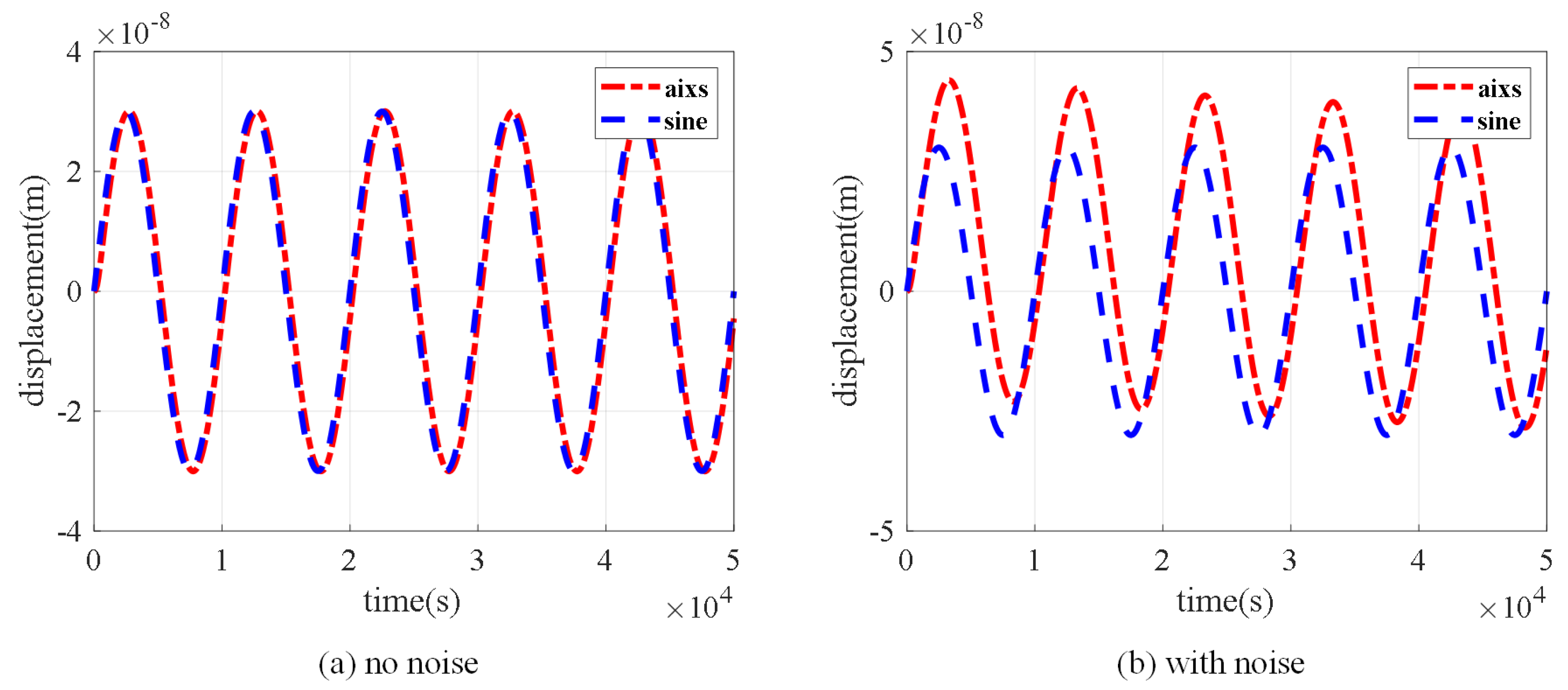
4. Simulation and Discuss

In this section, the previously proposed control method is verified by a series of simulated experiments through the TianQin model, whose ideal orbit is circular, and the semi-major axis parameter is r = 10 5 km . Assume the initial position and velocity of the spacecraft and TMs are p = [ 0   m , 0   m ] T , v = [ 0   m / s , 0   m / s ] T , respectively. Because the disturbance acted on spacecraft in space is mainly solar radiation pressure that is of minimal quantity, assume Ve is at 10 8 magnitude. The Drag-free spacecraft carries micro propulsion, so Vu is assumed at 10 4 magnitude. In order to simplify this model, the inner loop uses the same parameters as the outer loop. Regarding the actuator noise and disturbance, they uniformly use 10 9 magnitude. To sum up, we have
K 1 = 0.0003 4.5668 × 10 7 0.0343 7.0955 × 10 18 4.5668 × 10 7 0.0003 7.0955 × 10 18 0.0343 6.4859 × 10 14 8.1725 × 10 17 1.4999 3.9603 × 10 27 8.1725 × 10 17 6.4859 × 10 14 3.9603 × 10 27 1.4999 T
K 2 = 1271 × 10 4 2.1452 1080 × 10 2 3.5709 × 10 10 2.1454 1271 × 10 4 2.0884 × 10 10 1080 × 10 2 29.6746 6.6837 × 10 6 0.0013 4.2445 × 10 14 6.6837 × 10 6 29.6746 4.2445 × 10 14 0.0013 T
Figure 7a shows the spacecraft, which is comprised of the outer-loop tracking step signal, where the red and blue lines denote the displacement of the spacecraft, and the green line denotes the tracking signal. The first two lines and the third line had a better fit, and the error is less than the magnitude. Figure 7b shows the TMs, comprised of the inner-loop tracking ideal orbit. The curves fit better than the outer loop and drop gradually to 0 when the step signal stabilizes, which conforms previously designed property.
Figure 8 shows the tracking effect of the outer loop at different frequencies, where (a), (b) shows it has a good tracking effect in the low-frequency band, and (c), (d) shows it has no-tracking at high frequency. This verifies that this controller can meet the requirement of control signal filtering in the high-frequency band.
Figure 9 shows the tracking effect of inner loop at different frequencies, where (a), (b) shows it does not track in the low-frequency band, and (c), (d) shows it has tracking at high frequency. This verifies that this controller has good properties of control-signal filtering in the low-frequency band.
Then, the merit of robustness of the control method in this paper is presented and discussed as follows. In order to show the difference between this controller and the traditional mixed-sensitivity controller, which is H based on the small gain theorem, a contrast figure is shown as follows.
Figure 10a shows the tracking effect of an outer loop that uses a frequency-domain-based control strategy. It can be seen that the axis has tracking sine disturbance. However, looking to Figure 10b, it is obvious that the curve has a large tracking error when the actuator is impacted by external noise.
Figure 11 shows the tracking effect of the outer loop at 0.01 mHz with the actuator noise and the disturbance of different frequencies.
Figure 12 shows the tracking effect of the inner loop at 3 Hz with the actuator noise and the disturbance of different frequencies.
Figure 11 and Figure 12 show it has still good tracking with the tracking-frequency noise and no-tracking-frequency noise of the actuator. This indicates that the controller has good robust stability when the system has mixed disturbance.

5. Conclusions

The mixed-sensitivity control of a drag-free spacecraft with systems of drag-free and electrostatic suspension have been investigated in this paper. The tracking error has been separated according to the high or low frequency of disturbances. Then, the CW equations of TMs with respect to the ideal orbit and the center of cavity with respect to TMs have been devised. Furthermore, we have developed two mixed-sensitivity controllers of the MIMO system based on state feedback in state space for drag-free and electrostatic suspension, respectively, which have the advantages of overcoming the disturbances and noise of the system. Finally, the performance of the controllers has been demonstrated by a simulation experiment.

Author Contributions

Conceptualization, C.J.; methodology, C.J.; software, C.J.; writing—orginal draft preparation, C.J.; writing—review and editing, Y.L.; supervision, Y.L.; funding acquisition, Y.L. All authors have read and agreed to the published version of the manuscript.

Funding

This research was funded by The Central University Basic Research Fund of Sun Yat-sen University (19lgpy280).

Data Availability Statement

Not applicable.

Conflicts of Interest

The authors declare no conflict of interest.

References

  1. Reigber, C.; Lühr, H.; Schwintzer, P. CHAMP mission status. Adv. Space Res. 2002, 30, 129–134. [Google Scholar] [CrossRef]
  2. Michaelis, I.; Styp-Rekowski, K.; Rauberg, J.; Stolle, C.; Korte, M. Geomagnetic data from the GOCE satellite mission. Earth Planets Space. 2022, 74, 1–16. [Google Scholar] [CrossRef]
  3. Cesare, S.; Allasio, A.; Anselmi, A.; Dionisio, S.; Mottini, S.; Parisch, M.; Massotti, L.; Silvestrin, P. The European way to gravimetry: From GOCE to NGGM. Adv. Space Res. 2016, 57, 1047–1064. [Google Scholar] [CrossRef]
  4. Pelivan, I. Dynamics and control modeling for gravity probe B. Space Sci. Rev. 2010, 151, 5–23. [Google Scholar] [CrossRef]
  5. Overduin, J.; Everitt, F.; Mester, J.; Worden, P. The science case for STEP. Adv. Space Res. 2009, 43, 1532–1537. [Google Scholar] [CrossRef]
  6. Bergé, J.; Baghi, Q.; Hardy, E.; Métris, G.; Robert, A.; Rodrigues, M.; Touboul, P.; Chhun, R.; Guidotti, P.-Y.; Pires, S.; et al. MICROSCOPE mission: Data analysis principle. Class. Quant. Grav. 2022, 39, 204007. [Google Scholar] [CrossRef]
  7. Abbott, B.P.; Abbott, R.; Abbott, T.D.; Abernathy, M.R.; Acernese, F.; Ackley, K.; Adams, C.; Adams, T.; Addesso, P.; Adhikari, R.X.; et al. Observation of gravitational waves from a binary black hole merger. Phys. Rev. Lett. 2016, 116, 061102. [Google Scholar] [CrossRef] [Green Version]
  8. Amaro Seoane, P.; Arca Sedda, M.; Babak, S.; Berry, C.P.; Berti, E.; Bertone, G.; Blas, D.; Bogdanović, T.; Bonetti, M.; Breivik, K.; et al. The effect of mission duration on LISA science objectives. Gen. Relativ. Gravit. 2022, 54, 1–47. [Google Scholar] [CrossRef]
  9. Luo, J.; Chen, L.S.; Duan, H.Z.; Gong, Y.G.; Hu, S.; Ji, J.; Liu, Q.; Mei, J.; Milyukov, V.; Sazhin, M.; et al. TianQin: A space-borne gravitational wave detector. Class. Quant. Grav. 2016, 33, 035010. [Google Scholar] [CrossRef] [Green Version]
  10. Lange, B. The drag-free satellite. AIAA J. 1964, 2, 1590–1606. [Google Scholar] [CrossRef]
  11. Space Department of Johns Hopkins Universitythe GuidanceControl Laboratory of Stanford University. A satellite free of all but gravitational forces: “TRIAD I”. J. Spacecr. Rocket. 1974, 11, 637–644. [Google Scholar] [CrossRef]
  12. Armano, M.; Audley, H.; Baird, J.; Binetruy, P.; Born, M.; Bortoluzzi, D.; Castelli, E.; Cavalleri, A.; Cesarini, A.; Cruise, A.M.; et al. LISA Pathfinder platform stability and drag-free performance. Phys Rev. D 2019, 99, 082001. [Google Scholar] [CrossRef] [Green Version]
  13. Hu, Z.; Wang, P.; Deng, J.; Cai, Z.; Wang, Z.; Wang, Z.; Yu, J.; Wu, Y.; Kang, Q.; Li, H.; et al. The drag-free control design and in-orbit experimental results of “Taiji-1”. Int. J. Mod. Phys. A 2021, 36, 2140019. [Google Scholar] [CrossRef]
  14. Leach, R. Development of hardware for a drag-free control system/Gravitational-Wave Detection. SPIE 2003, 4856, 19–30. [Google Scholar]
  15. Wu, S.F.; Fertin, D. Spacecraft drag-free attitude control system design with quantitative feedback theory. Acta Astronaut. 2008, 62, 668–682. [Google Scholar] [CrossRef]
  16. Zou, X. Calibration of the Satellite Gravity Gradients for GOCE and Analysis on Its Drag Free Control System. Acta Geod. Cartogr. Sin. 2018, 47, 291. [Google Scholar]
  17. Gath, P.; Fichter, W.; Kersten, M.; Schleicher, A. Drag Free and Attitude Control System Design for the LISA Pathfinder Mission. In Proceedings of the AIAA Guidance, Navigation, and Control Conference and Exhibit, Providence, RI, USA, 16–19 August 2004; p. 5430. [Google Scholar]
  18. Wang, E.; Qiu, S.; Liu, M.; Cao, X. Event-triggered adaptive terminal sliding mode tracking control for drag-free spacecraft inner-formation with full state constraints. Aerosp. Sci. Technol. 2022, 124, 107524. [Google Scholar] [CrossRef]
  19. Lian, X.; Zhang, J.; Chang, L.; Song, J.; Sun, J. Test mass capture for drag-free satellite based on RBF neural network adaptive sliding mode control. Adv. Space Res. 2022, 69, 1205–1219. [Google Scholar] [CrossRef]
  20. Zou, K.; Gou, X. Characteristic model-based all-coefficient adaptive control of the drag-free satellites//2020 Chinese Automation Congress (CAC). Shanghai, China, 6–8 November 2020; 2020; pp. 2839–2844. [Google Scholar]
  21. Huang, W. Single Mass Drag-Free Control Based on the High-Gain Observer, 3rd ed.; Harbin Institute of Technology: Harbin, China, 2021; pp. 21–35. [Google Scholar]
  22. Fichter, W.; Schleicher, A.; Szerdahelyi, L.; Theil, S.; Airey, P. Drag-free control system for frame dragging measurements based on cold atom interferometry. Acta Astronaut. 2005, 57, 788–799. [Google Scholar] [CrossRef]
  23. Canuto, E.; Colangelo, L.; Buonocore, M.; Massotti, L.; Girouart, B. Orbit and formation control for low-earth-orbit gravimetry drag-free satellites. Proc. Inst. Mech. Eng. Part J. Aerosp. Eng. 2015, 229, 1194–1213. [Google Scholar] [CrossRef] [Green Version]
  24. Lian, X.; Zhang, J.; Wang, J.; Wang, P.; Lu, Z. State and disturbance estimation for test masses of drag-free satellites based on self-recurrent wavelet neural network. Adv. Space Res. 2021, 67, 3654–3666. [Google Scholar] [CrossRef]
  25. Wang, E.; Zhang, J.; Li, H.; Liu, M. Relative Position Model Predictive Control of Double Cube Test-Masses Drag-Free Satellite with Extended Sliding Mode Observer. Math. Probl. Eng. 2021, 2021, 1–15. [Google Scholar] [CrossRef]
  26. Tan, S.; Guo, J.; Zhao, Y.; Zhang, J. Adaptive control with saturation-constrainted observations for drag-free satellites—A set-valued identification approach. Sci. China Inform. Sci. 2021, 64, 1–12. [Google Scholar] [CrossRef]
  27. Lian, X.; Zhang, J.; Lu, L.; Wang, J.; Liu, L.; Sun, J.; Sun, Y. Frequency separation control for drag-free satellite with frequency-domain constraints. IEEE Trans. Aerosp. Electron. Syst. 2021, 57, 4085–4096. [Google Scholar] [CrossRef]
  28. Theis, J.; Pfifer, H. Observer-based synthesis of linear parameter-varying mixed sensitivity controllers. Int. J. Robust. Nonlin. 2020, 30, 5021–5039. [Google Scholar] [CrossRef]
  29. Theis, J.; Sedlmair, N.; Thielecke, F.; Pfifer, H. Observer-based LPV control with anti-windup compensation: A flight control example. IFAC-PapersOnLine 2020, 53, 7325–7330. [Google Scholar] [CrossRef]
  30. Wu, F. Control of Linear Parameter Varying Systems, 3rd ed.; University of California: Berkeley, CA, UDA, 1995; pp. 31–50. [Google Scholar]
  31. Theis, J.; Pfifer, H.; Seiler, P. Robust modal damping control for active flutter suppression. J. Guid. Control. Dynam. 2020, 43, 1056–1068. [Google Scholar] [CrossRef]
Figure 1. Reference frame.
Aerospace 09 00708 g001
Figure 2. Relative error of drag-free spacecraft.
Aerospace 09 00708 g002
Figure 3. Block diagram of mixed-sensitivity control.
Aerospace 09 00708 g003
Figure 4. Sensitivity of We−1.
Aerospace 09 00708 g004
Figure 5. Sensitivity of We−2.
Aerospace 09 00708 g005
Figure 6. Block diagram of control system.
Aerospace 09 00708 g006
Figure 7. Tracking of step signal: (a) outer-loop, (b) inner-loop.
Aerospace 09 00708 g007
Figure 8. Tracking of sine signal for drag−free at (a) 1 μ Hz, (b) 0.01 mHz, (c) 10 mHz, (d) 1 Hz.
Aerospace 09 00708 g008
Figure 9. Tracking of sine signal for electrostatic suspension at (a) 1 μ Hz, (b) 1 mHz, (c) 3 Hz, (d) 10 Hz.
Aerospace 09 00708 g009
Figure 10. Tracking of drag−free using frequency-domain-based controller (a) with noise and (b) with no noise.
Aerospace 09 00708 g010
Figure 11. Tracking of drag−free with disturbance of (a) 1 μ Hz and (b) 1 Hz.
Aerospace 09 00708 g011
Figure 12. Tracking of electrostatic suspension with disturbance of (a) 1 μ Hz and (b) 10 Hz.
Aerospace 09 00708 g012
Publisher’s Note: MDPI stays neutral with regard to jurisdictional claims in published maps and institutional affiliations.

