Article

Multi-Domain Based Computational Investigations on Advanced Unmanned Amphibious System for Surveillances in International Marine Borders

by
Vijayanandh Raja
1,
Ramesh Murugesan
2,
Parvathy Rajendran
3,4,*,
Surya Palaniappan
1,
Hussein A. Z. AL-bonsrulah
5,6,
Darshan Kumar Jayaram
1 and
Mohammed Al-Bahrani
7,8
1
Department of Aeronautical Engineering, Kumaraguru College of Technology, Coimbatore 641049, Tamil Nadu, India
2
Design Engineer, MaDeIT innovation foundation, IIITDM, Kanchepuram 600127, Tamil Nadu, India
3
School of Aerospace Engineering, Universiti Sains Malaysia, Nibong Tebal 14300, Penang, Malaysia
4
Faculty of Engineering & Computing, First City University College, Bandar Utama, Petaling Jaya 47800, Selangor, Malaysia
5
Al-Amarah University College, Maysan 62001, Iraq
6
Iraqi Ministry of Oil, Midland Refineries Company, Najaf Refinery, Najaf 54001, Iraq
7
School of Engineering, University of Plymouth, Plymouth PL4 8AA, UK
8
Chemical Engineering and Petroleum Industries Department, Al-Mustaqbal University College, Babylon 51001, Iraq
*
Author to whom correspondence should be addressed.
Aerospace 2022, 9(11), 652; https://doi.org/10.3390/aerospace9110652
Submission received: 3 September 2022 / Revised: 17 October 2022 / Accepted: 20 October 2022 / Published: 26 October 2022
(This article belongs to the Special Issue Applications of Drones)

Abstract

:
The conceptual design, component selection, and deployment experiments of an unmanned amphibious system (US) with a unique Becker in vertical stabilizer based on hydrodynamic research are included in this work. The use of USs is currently expanding significantly, and they are used for fish detection, oceanographic mapping, mining detection, monitoring marine life, and navy purposes. With a maximum forward speed of 30 m/s, the US’s hull is largely built with criteria for identifying and researching marine species. The significant lifetime decline of ocean species drives the deployment of unmanned vehicles for species monitoring from the water’s surface to 300 m below the surface. In addition, the medical team can help the species with health problems using this planned US because they have been identified. The conceptual design and estimated analytical equations encompass the fuselage, Becker rudder, propeller, and other sub-components. The locations of sensors, primarily used to locate mobile marine life, are also considered. A Becker rudder has been imposed to make sharp turns when the US is submerged in water. An advanced hydro propeller produces the propulsion with a 20 cm base diameter. Additionally, a piezoelectric patching-based energy extracting approach is used to the hydro-outside propeller’s surface. As a result, the electrical power generation for different lightweight materials is computed for the performance of US manoeuvrings. With the help of CATIA modelling of the intended USs and ANSYS Fluent hydrodynamic simulations, appropriate high-speed configurations are selected. Various stages of its mission profile, including the US in steady-level flight, the US in climb, and the US over the ocean surface, are subjected to computational simulations. Using an advanced computational technique and previously established experimental correlations, the reliability of these various computational solutions is examined and kept at an appropriate level. This US is highly suggested for marine-based real-time applications due to its acceptable output.

1. Introduction

Recent years have seen an explosion in unmanned vehicles, which have endless potential uses. The three primary types of unmanned vehicles are based on aircraft, water, and ground working conditions. The paper focuses on the computational studies and unmanned vehicle designs of amphibians. Since unmanned amphibious vehicles must operate in both water and air, they provide unique challenges in design and production compared to traditional unmanned aquatic vehicles (UAVs). The challenges of designing a low-drag, highly agile, and quick unmanned underwater vehicle (UUV) are compounded by the density of seawater and the increase in pressure with an increase in depth. This study optimizes the design of an underwater vehicle from the standpoint of making it as quick and agile as possible while submerged. The UUVs are a type of UAV wherein such vehicles are employed in deep-sea environments where human participation is feasible. Underwater unmanned vehicles include ROVs (remotely operable vehicles) and UUVs. Many nations rely on unmanned underwater vehicles for various tasks, including marine operations, topological mapping, ocean bed mapping, and many more. UAVs have many potential uses, one of the most important being fish detection. A UAV’s primary function is to operate in water; hence it must be able to swim quickly, efficiently, and with good mobility. Underwater vehicles can be highly manoeuvrable and have low drag by following certain design principles. In this study, the authors examine the computational hydrodynamic behaviour of the novel unmanned amphibious vehicle designed to keep an eye on marine life and save sick or injured marine animals. The computational hydrodynamic analyses shed light on the development of drag over the unmanned amphibious system (US), the hydro propeller’s thrust force, and the upper force on the US, including the buoyancy force and the lift force. Through computational fluid dynamics-based single-moving reference frame (CFD-SMRF) methods, we can determine the optimal propeller and operating parameters for a level flight and the most robust material for withstanding the air and water. Finally, the targeted mission is continuous, so energy requirement is high in the US. Henceforth, the piezoelectric patching-based energy-extracting approach has been planned on the hydro-outside propeller’s surface for possible energy extractions.

1.1. Innovations of This Work

This work aims to design and computationally develop the flexible Unmanned Amphibious System with the help of advanced computational coupled approaches. The targeted application is to monitor an intruder’s presence and activities at the international marine border through this suggested advanced US. In this regard, the first cycle of the US’s mission profile is planned and revealed in Figure 1, wherein the working function is continuous monitoring of illegal entries of intruders in and around the international marine borders.

1.2. Literature Survey

This section primarily focused on four areas: the first dealt with typical designs used in unmanned vehicles, the second dealt with CFD research on unmanned vehicles, the third dealt with FEA (finite element analysis) computations on unmanned vehicles, and the fourth dealt with energy extraction on unmanned vehicles. The relevant articles are: Wang Qinyang et al. described an underwater vehicle in which float bowls and spinning wings helped it fly and float. Whirling wings increase airlift and decrease water resistance by reducing surface tension. UUV float bowls allow water to be introduced, increasing the UUV’s density and submergibility. CFD examined aerodynamic and hydrodynamic performance. The whirling wings improved water performance [1]. Yongcheng Li et al. examined an autonomous underwater vehicle (AUV)’s performance in the water. This AUV has biology-inspired undulating wings. This article compared aspect ratio to thrust power and efficiency. They also covered how AUV vortex formations altered with different aspect ratios. Thrust force and propulsive efficiency rose with the aspect ratio [2]. James Louis Tangorra et al. considered fish a basis for an AUV propeller. Due to its complexity, they studied the Bluegill sunfish’s pectoral fin. This study examined sunfish pectoral fins’ morphology, hydrodynamics, and kinematics. Findings showed that its fins are unique. Dimples and leading-edge vortices increased thrust. This research showed that a robotic fin had been used to propel UUVs in the future, increasing their agility [3]. Tae-Hwan Joung et al. conceptualized an AUV in which they focused on hull resistance as the main factor affecting AUV power consumption and range. CFD analysis determined the hull’s hydrodynamic resistance. Next, a ducted propeller optimized the AUV’s design while CFD analysed it. Ducted propellers reduce body load [4]. Gang Xuel et al. analysed fish motion models. Tuna was a study model that employed fish movement to test three motion models. The first model was the undulatory model with an exponential function, then the oscillating model with a polynomial, and finally, the undulatory model with a polynomial. Each model’s characteristics and hydrodynamic efficiency were analysed numerically. Higher amplitude is preferable to higher frequency [5]. Amy Gao et al. developed aerial and underwater robotic watercraft. This contraption mimics the flying fish’s ability to avoid predators. The authors utilized math to investigate the robotic fish’s hydrodynamic properties and mechanical design approaches. A mechanical replica was developed and tested to evaluate how closely the robotic fish matched the actual fish. These insights were used to develop future-proof conceptual ideas [6].
Wang Zihao et al. analysed a flying-wing underwater glider. Due to underwater gliders’ low lift-drag ratio, this glider has flying wings. This study used math and CFD to assess a flying wing design. Design optimization enhanced gliding performance [7]. Vijayakumar Mathaiyan et al. evaluated a remote-controlled amphibious vehicle. The flying fish’s glide ratio inspired this design. Innovative design lets it swim and fly. A retractable wing reduced the UAV’s water profile and flying resistance. CFD and fluid-structure interaction (FSI) investigated five lightweight materials. The epoxy-E-glass-fabric composite showed excellent hydrodynamic performance [8]. Muhammad Yasar Javaid et al. examined underwater glider wing designs’ hydrodynamics and dynamic stability. Rectangular and tapered wing forms were used. Tow tank and CFD analysis tested the glider’s efficiency. The rectangular wing design produced tremendous lift forces but developed unstable. Tapered wings had a poor lift but good dynamic stability [9]. Khairul Alam et al. provided an AUV design optimization approach to reduce drag, power consumption, and operational costs. Adding modules to the framework helps the developer manage and optimize size and complexity. ANSYS ICEM and Fluent solve problems. This framework’s versatility is shown by its ability to identify the most promising early AUV designs. The framework’s production process and tools ensure high-quality and reliable components [10]. V Praveen Kumar et al. designed and assessed an unmanned watercraft. The design was inspired by flying fish and built through underwater concepts. After the design, CFD determined the UAV’s hydrodynamic performance. In this analysis, a cylinder-shaped hull was used. CFD analysed pressure, velocity, and drag [11]. Kondeti Lakshmi Vasudev introduced underwater vehicles (UV) and examined submarines, AUVs, manned UVs, ROVs, and towed instrument packages. All simulations employed 3D steady-state segregated RANS. CFD is useful for hydrodynamic UV design since it has saved costs and development time. CFD solvers determined drag and wave resistance. The military used AUVs to search the deep oceans [12].
Osman Md Amin et al. described ROVs and AUVs as the two main UUV classifications. The author highlighted underwater vehicle mobility, vital for manoeuvring around obstacles, laying pipes, searching for resources, destroying mines, and conducting oceanographic surveys. Creating a six-degree-of-freedom (DOF) UUV control system was the goal. Through CFD, researchers improved the propeller and constructed a low-drag hull. Roll, one-point rotation, glide, spiral, drift, hover, and zigzag-based manoeuvrings were tested [13]. R. Sankaresh Pandian et al. described a UAV with long operatable life, efficient construction, dependable flight, and low maintenance expenses. The authors scaled back the design’s demanding aspects through CFD simulations. ANSYS-Fluent solved CFDs. A stingray-inspired construction and symmetric aerofoil preserved the UAV’s water stability. The best UAVs were examined with CFD software before deployment [14]. Nesteruk, G. Passoni et al. estimated the power needed to propel a robotic fish similar toa genuine one and the drag. Swimming similar toa fish is hard and unstable. Therefore, a robot fish must be well-designed and powerful to mimic fish motion. The authors’ studied a bottle-nose dolphin’s drag, velocity, boundary layer, and other parameters. Animal morphologies and locomotion could help develop robot fish and underwater vehicles. The robotic fish should have a streamlined shape that ensures a flow pattern and a laminar boundary layer [15]. Mark C. Bettlea et al. suggested an implicit predictor-corrector method for simultaneously integrating the six DOF equations of motion for a manoeuvring submarine and the unsteady Reynolds-Averaged Navier Stokes (URANS) equations described vehicle hydrodynamics, provides a novel approach to the study of submarine manoeuvring. ANSYS CFX solved CFDs. Mesh perfectly covered submarines. A predictor-corrector approach was utilized to model emergency risers and horizontal zigzags for 6 DOF URANS submarine simulations. Due to stability limits on the relief parameter in fixed-point iteration, increasing the time step size was inefficient [16]. Yanhui Wang et al. described the design of a movable-wing hybrid underwater glider. The angle of attack and sweep angle can be changed for different motion types. This AUV can be low-cost and useful marine observation platforms due to their compact design, long operational life, and capacity to collect oceanographic data. Different wing configurations were simulated in glide, spiral, and horizontal turns and improved flight simulations. The moveable wing has been found to improve flight performance. They found that AUVs are a cost-effective alternative to manned vessels for underwater search and survey tasks [17]. Qiu Suming et al. analysed issues peculiar to UUVs, including form, wing, cross-domain, and take-off and landing design. AUV operation was difficult because it had been operated in air and water. They explored bioinspired underwater AUVs. They discussed prototypes and uses. Several types of AUVs were covered and tackled design issues such as control, take-off and landing, and communication [18].
Wang, Zhi-Jun et al. outlined the processes needed to develop a free-moving robot dolphin-like underwater vehicle. Three-dimensional motion analysis was used to examine oscillation frequency and forward motion. Due to its dolphin-like look, the fish’s body traits were classed. Body size was a factor. The AUV’s capacity to float and dive results from its control system and physical mechanics, wherein the centre of gravity and pitch angle were investigated [19]. Franz Uiblein et al. proposed a design for an amphibious unmanned surface vehicle for the marine SAR system. A sea-and-air propulsion module was envisioned. The strategy aforesaid was improved cruise efficiency and ease. This work compared the pros and cons of unmanned watercraft. Flying, hovering, and navigating on the ground were explained. The aircraft’s actual mechanical construction was carefully built, and its flight posture was analysed. This study proposed a conceptual design and guidelines for increasing rescue and search vehicle performance [20]. Meliha Bozkurttas et al. focused on fish’s various skills. The contrast between spontaneous and induced behaviour was the most important in ecology. “Situ exploration” offered information about fish at depths 200 m or less. Their behaviour was compared to shallow-water species. Next, researchers analysed habitat utilization and movement. The case study used 10 sea-bed video transects. Round-nose grenadier, orange roughly, and artificial boarfish were studied [21]. Frank E Fish designed and tested a Bluegill sunfish-inspired AUV’s propeller. Their skeletons allowed them to swim and move. Hydrodynamically, the fish’s pectoral fin was used as a baseline for AUVs’ flexible propellers [22].
The six-pronged technique and 3D kinematic patterns were studied during steady-forward swimming. Next, fin flow patterns were analysed computationally. Finally, the knowledge was used to design a bio-robotic fin propulsor [22]. Wang, Junshi et al. studied about six flying fish families (Exocoetidae) and investigated their morphology and aerodynamics. First, fins were morphed into glider-like wings to improve their flight. The imposed scaled flight factors were aspect ratio and wing loading. The improved wing had a high lift and low drag. Next, fin size was compared to wing area, wingspan, wing loading, and aspect ratio to body size. The outcome considered data from other flyers and gliders [23].
Llanez, Ignacio et al. studied fish finlets, wherein short, non-folding fines were imposed. Mackerels, bonitos, and tunas have them. Species swam well also they combined experimental and computational methods to determine finlet hydrodynamics. Through high-speed films, fluid motion in vivo was investigated. Wake hydrodynamics were examined by revealing underlying vortex formations. Finally, kinematically and anatomically precise finlet models were constructed using yellowfin tuna video data [24]. Park H et al. aimed to offer an optimum design for a Caribbean-focused AUV. Deep sea divers’ risks constitute a barrier to human exploration. Due to deep water pressures, AUV hull performance was a top priority. The hull was designed to withstand harsh conditions while minimizing hydrodynamic drag. The hull’s water resistance was determined using CFD and empirical methods. Drag prediction was affected. This research presented a revolutionary design for the AUV’s torpedo body, giving new possibilities for deep-water operations [25]. Benedetto Allotta et al. investigated flying fish, referred to as Exocoetidae. Some flying marine creatures can swim and fly. Their aerodynamic shape allowed them to glide despite these limits. Researchers first explored morphological and behavioural adaptations for flight and aerodynamics. This article examined the relationship between fish fin morphology and aerodynamic pressures. Fins improved lift and reduced drag. Additionally, this work examined the aerodynamic forces per ton in the ground effect, which can be exploited to reduce drag by flying low [26]. Ting Gao et al. outlined the design and development of a self-driving underwater vehicle called “Tifone” The Thesaurus work includes this study. Its deliberate design lets it perform high-profile duties. It can withstand 300-m water pressure and 5-knot winds. It is similar toa torpedo from the perspective of Fluid dynamics. Commonly, lateral and vertical thrusters were used as control surfaces. This makes the system more stable and reduces malfunctions [27].
Calculations based on computational fluid dynamics were employed as a relay in the computational methods used to accommodate the rotodynamic effect. We took readings on things such asthe density and viscosity of the fluid, among other things. As a result of the significant impact load that the fluids supply, the stable flights of the UUV are at an increased risk of collision while it is flying through the fluid. Investigations using CFD and FEA were a part of the currently underway work process. Due to this reason, the literature reviews that were based on the finite element analysis have been completed. The primary focus of supervision is on lightweight materials with strong mechanical capabilities that can endure the loads caused by the ocean. A comprehensive investigation into the locations and particulars of both stationary and far-off dislocations was carried out. Testing the convergence of the grid allowed us to monitor the various types of grid generation as well as the overall quality of the grid. In conclusion, our research considered the structural results that were concerned in the selection process were taken into consideration [28,29,30,31,32,33,34]. Finally, the studies on energy extraction by US propellers through piezoelectric patches were examined. The analytical calculations involved in estimating electrical voltage development through piezoelectric patches were found. The mechanical and dielectric properties of various imposed lightweight materials were obtained. [35,36,37,38,39,40,41,42,43,44,45,46,47].

1.3. Author Observation and Finalization

Most unmanned amphibious systems are geometrically developed fuselages with different fins for their manoeuvrings. Nevertheless, this work is finalized to replace a rectangular wing instead of horizontal fins and to impose a Becker rudder rather than vertical fins. Finally, an advanced hydro propeller is planned to design based on the mission’s thrust requirement and the dimensions of the Becker rudder. This work majorly relays advanced computational approaches such as computational hydrodynamic investigations, computational hydro-structural investigations, and computational vibrational investigations, wherein all the suitable conditions and experimental correlations for validations are extracted through this literature survey. Furthermore, to achieve continuous surveillance, this work planned to incorporate a piezoelectric energy generator on this US propeller, so integrated approaches were also studied to estimate electrical energy. All the computational models are planned to develop in CATIA and then proposed to examine in the ANSYS Workbench tool before discussing the optimal design.

2. Proposed Methodology—Computational Hydrodynamic Analysis

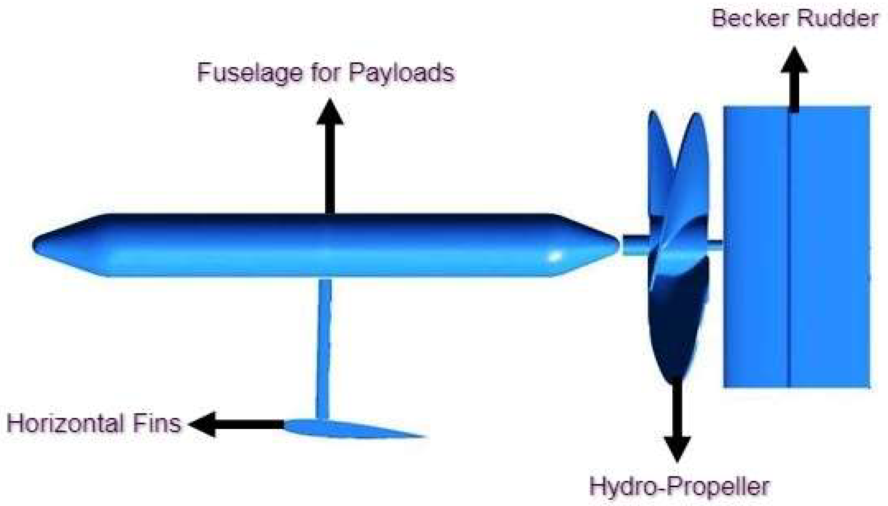
2.1. Design of Unmanned System

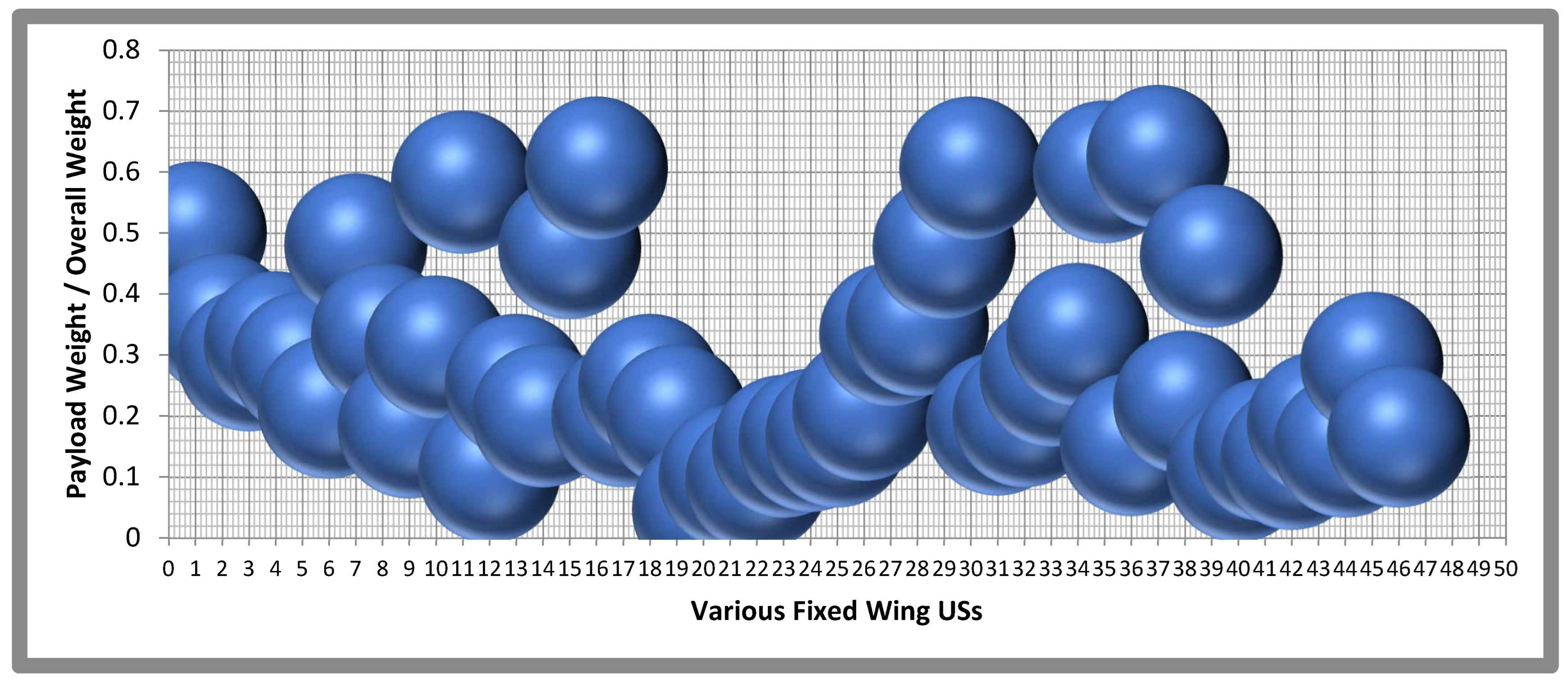
2.1.1. Design of Preliminary Calculations of Flexible Rectangular Wing

An estimate of the UAV’s overall mass can be made using Equation (1), which is based on past relationships (Figure 2) between important variables such aspayload weights and empty weights [28,29,30,31,32,33,34].
W Payload W Overall = 0.30 .
The major goal is to install and operate a system that continuously monitors marine species’ life from the ocean’s surface to a depth of 300 m. In addition, the US also supports the necessary adjustments for sick marine species. The planned flight employed a payload weight of 1 kg [28,29,30,31,32,33,34].
W Overall = W Payload 0.30 1 0.30 = 3.34   kg
High loading UAVs have wing loading values greater than 100 kg/m2, medium loading UAVs have wing loading values ranging between 50 kg/m2 and 100 kg/m2, and low loading UAVs have wing loading values less than 50 kg/m2. Consider the wing loading to be 50 kg/m2. The total weight is,
S Wing = W o W S 3.34 75 0.044534   S Wing = 0.044534   m 2
For this case aspect ratio of the flexible wing is assumed as,
AR Wing = b Wing 2 S Wing 10 = ( b Wing ) 2 S Wing b Wing = 0.044534 × 8 b Wing = 0.6   m
A well-stabilized structure has to be between 70 and 80%of its wingspan, but a denser fluid, such as hydro medium, can produce more lift. As a result, the “   ƞ “ is assumed to be 0.65 [28,29,30,31,32,33,34].
L Fuselage = ƞ × b Wing 0.65 × 0.6   L Fuselage = 0.40   m
The fineness ratio (FR) is assumed to be 10. Therefore,
FR = L Fuselage D Fuselage D Fuselage = L Fuselage FR = 0.40   10 = 0.04   m
From the standard equation,
S Wing = b Wing × C Wing Root
0.044534 = 0.6 × C Wing Root C Wing Root = 0.0743   m
Finally, the designs of preliminary calculations of flexible rectangular wing are calculated with the help of Equations (1)–(6). The typical top view-based representation of US rectangular wing is revealed in Figure 3.

2.1.2. Design of Vertical Stabilizer with Becker Rudder

A special rudder is chosen and imposed for this task to accomplish the yawing in a swift and responsive manner. Since the Becker rudder is more massive than standard rudders, it was decided that the vertical stabilizer’s planform area should be 30% of the wing’s planform area [28,29,30,31,32,33,34]. Aerodynamicists determine a wing’s area by measuring its surface above (top view-based projection). It is also possible to refer to this region as the “planform area,” which describes its shape. When figuring out how fast an aeroplane (US) will go, you need to know the planform area. Additionally, it is decided that the vertical stabilizer’s direction should be determined by both the rudder’s up and down design. Equations (7)–(9) contain the analytical approaches of Becker rudder’s design data.
S wing = 0.044534   m 2 S V Tail = 0.30 × S wing = 0.30 × 0.044534 = 0.0133602   m 2
S V Tail of   upper   component = 0.0133602 2 = 0.00668   m 2
S V Tail of   lower   component = 0.0133602 2 = 0.00668   m 2
b V Tail = ( AR V Tail × S V Tail ) 1 2
b V Tail ( 3 × 0.0133602 ) 1 2 b V Tail = 0.2   m
S V Tail = b V Tail × C V Tail root C V Tail root = S V Tail b V Tail
C V Tail root = 0.0133602 0.2 = 0.0668   m  
Since it has a low drag coefficient, the aerofoil “NACA 0012” is selected as the best alternative according to the literature review [37,38,39,40,41].

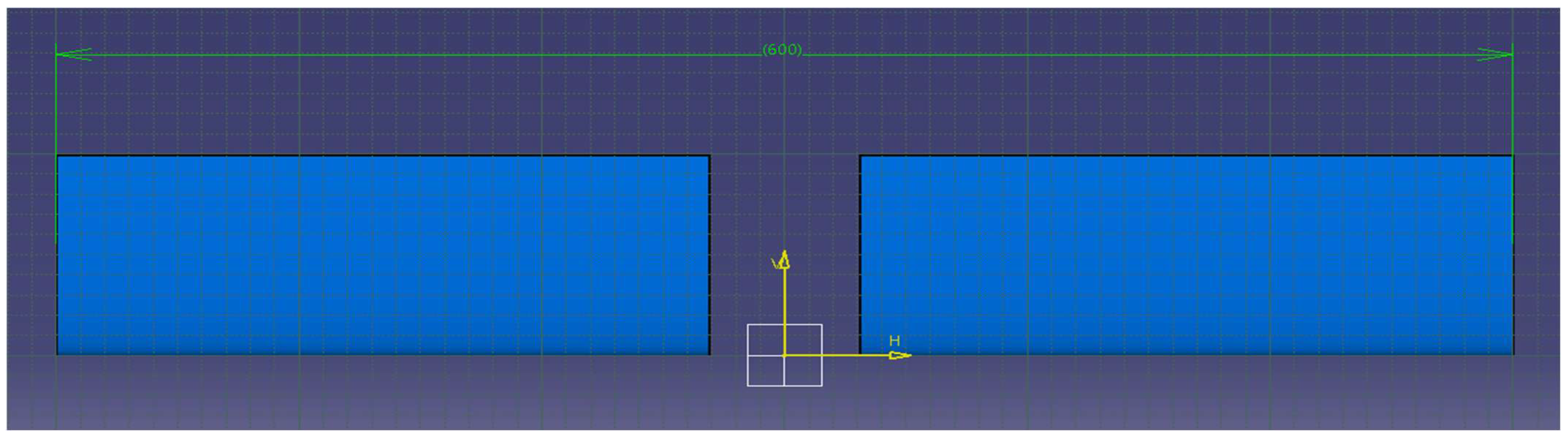
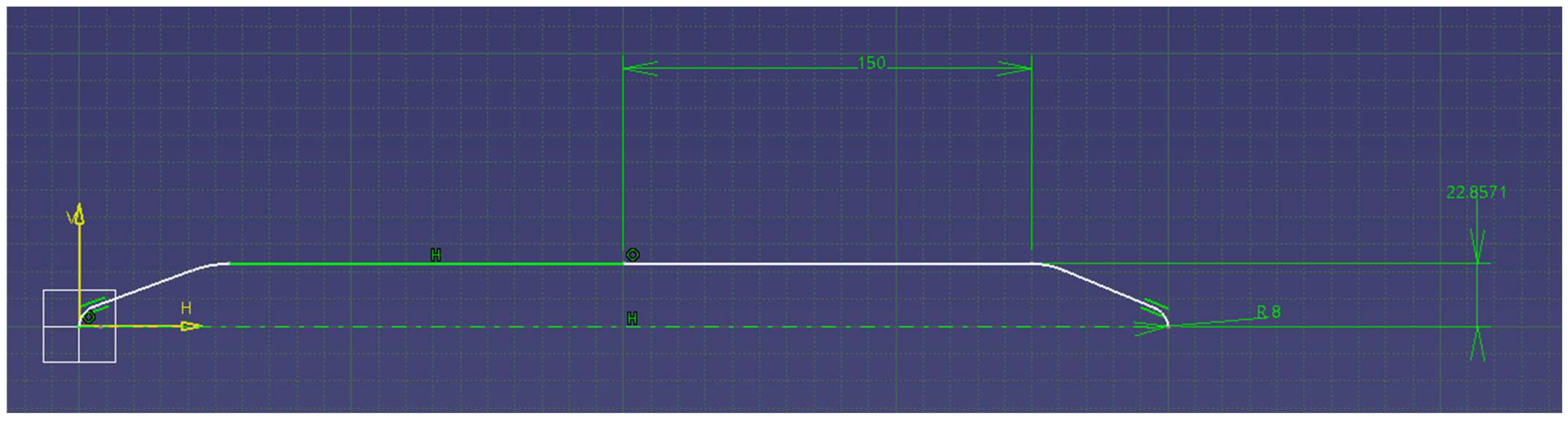
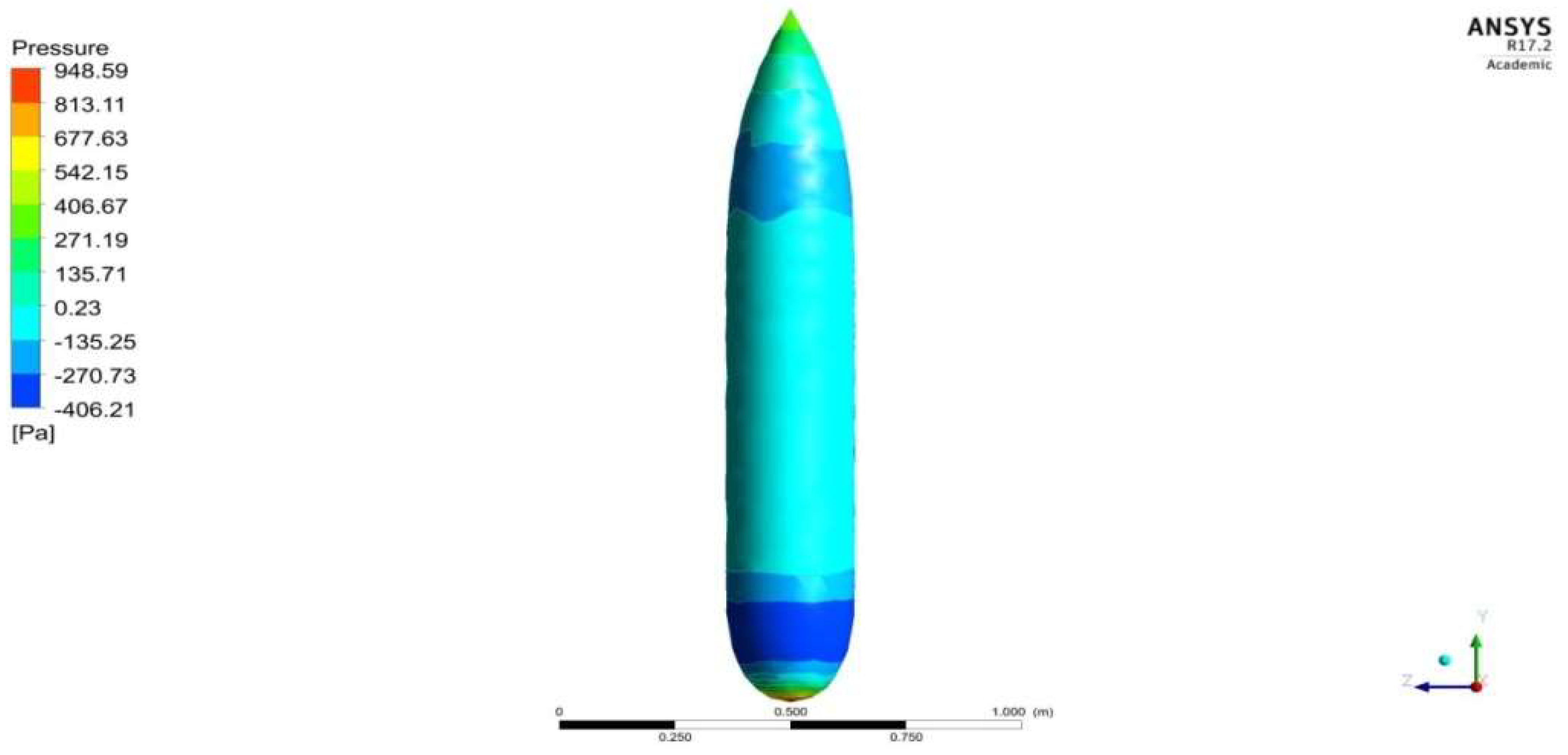
2.1.3. Fuselage Design

The planned US fuselage dimensions result from cutting-edge research on optimal aspect and fineness proportions [28,29,30,31,32,33,34]. The dynamic, relevant proportions are mentioned in Equations (10)–(13).
D Fuselage Maximum L Fuselage = 0.115
D Fuselage Maximum 0.4 = 0.115 D Fuselage Maximum = 0.115 × 0.4 D Fuselage Maximum = 0.046   m
L Fuselage Uniform   Cross   Section L Fuselage = 0.75
L Fuselage Uniform   Cross   Section 0.4 = 0.75 L Fuselage Uniform   Cross   Section = 0.75 × 0.4 L Fuselage Uniform   Cross   Section = 0.3   m
L Fuselage Varying   Cross   Section L Fuselage = 0.25
L Fuselage Varying   Cross   Section 0.4 = 0.25 L Fuselage Varying   Cross   Section = 0.4 × 0.25 L Fuselage Varying   Cross   Section = 0.1   m
D Fuselage Varying   Cross   Section = ( m × L Fuselage Varying   Cross   Section ) + b
After the successful estimations of primary design data of the US fuselage, the typical configuration is modelled with the help of CATIA. The final models of US fuselage are typically revealed in Figure 4 and Figure 5.

2.1.4. Propulsive System Design
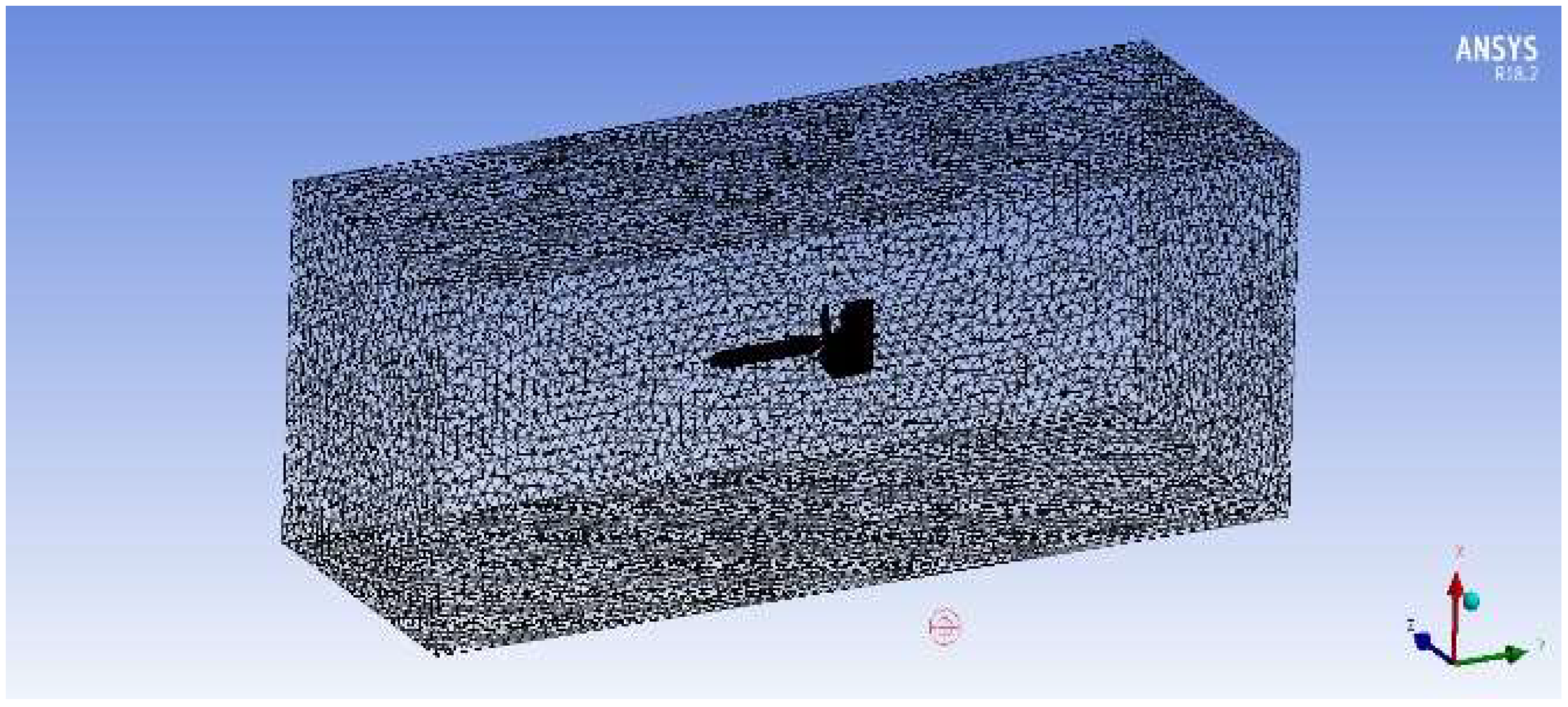
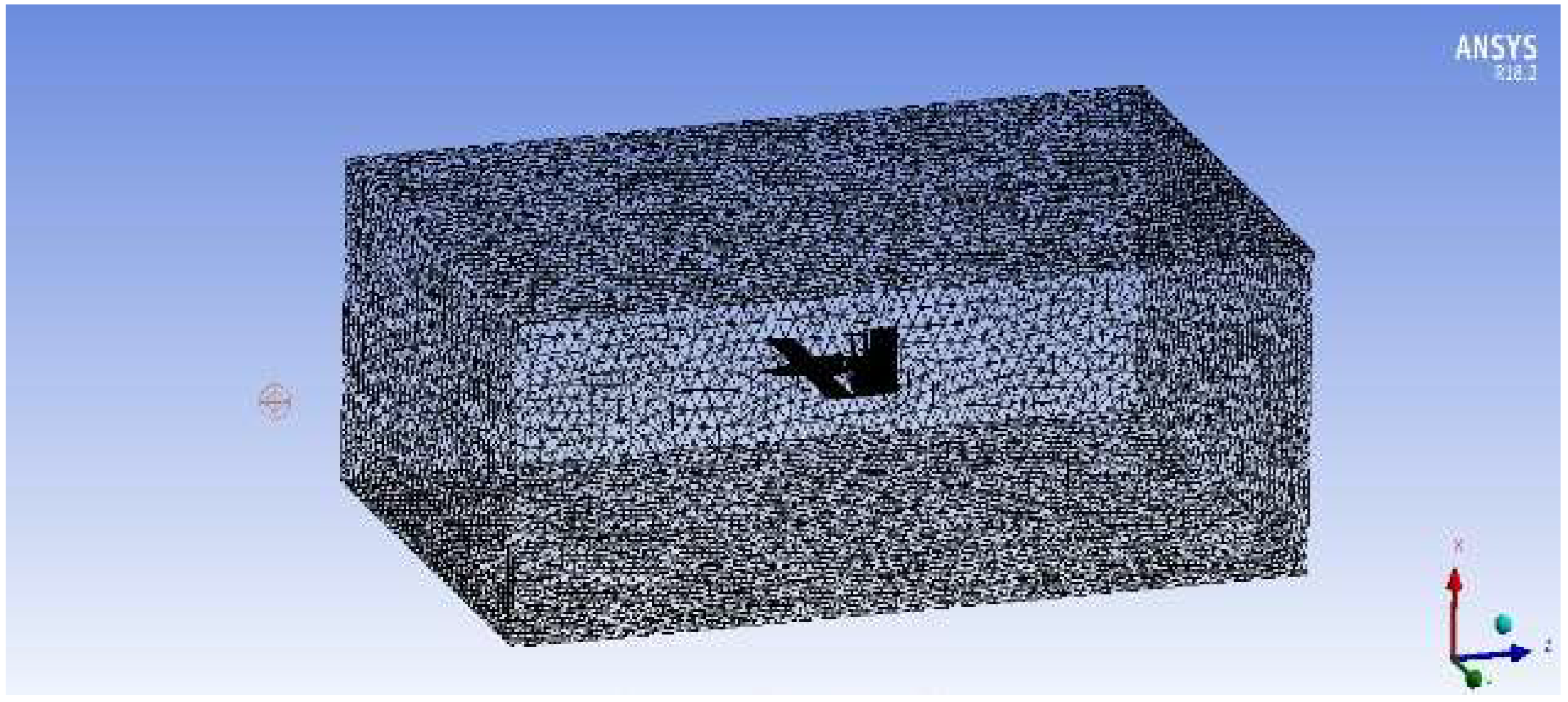
This sophisticated unmanned system’s propulsive design is more involved than that of conventional amphibious vehicles due to its US positioning. This US can yaw by using the increased thrust provided by its propeller. Equations (14)–(17) [28,29,30,31,32,33,34] serve as a foundation for the development of this propeller’s design, incorporating both contemporary and traditional mathematical techniques. The design methodologies for a marine propeller are proposed [28,29,30,31,32,33,34] after an extensive literature review. Diameter, delivered power, power coefficient, and hydrostatic and hydrodynamic velocities play important roles in the design’s foundation. Relationships between the planned power, the optimum diameter, the optimal speed ratio, and the position of the sectional chord length are given by Equations (14)–(17) [28,29,30,31,32,33,34].
T Required = { B T × [ ( V FS ) 5 2 ] N } 2 V FS
D Optimum = λ Optimum US , P × V FS N
λ Optimum US , P = { 100 [ B T 36.76 B T + ( 75.11 B T ) + 155.3 ] 0.2 × [ 0.9365 + 1.49 n US , P { ( 2.101 n US , P 0.1478 ) 2 × A E A O } ] }
C x % D US ,   P = K 0 US ,   P ( 1 r x % R US , P ) + K 1 US ,   P + K 2 US ,   P ( 1 r x % R US , P ) + K 3 US , P ( 1 r x % R US , P ) 2 + K 4 US , P ( 1 r x % R US , P ) 4 + K 5 US , P ( 1 r x % R US , P ) 5
The historical relationships are executed to attain the unknown design data of US propellers, such as pitch and thickness, so the relevant relationships are found. The functional relationships are mentioned in Equations (18) and (19). Finally, the modelled hydro propeller is systematically revealed in Figure 6.
Pitch   [ P ] = 0.87 × Diameter   [ D Optimum ]
Thickness   [ T ] = 0.323 × Pitch   [ P ]
Standard mathematical methods are being used to perfect the design of the pivoting wing, fuselage, and vertical stabilizer with Becker rudder that make up this US. In addition to these parts, the aerofoil is crucial in the design stage because it has generated an additional force, which will destroy the stability of a US. As a result, a symmetrical aerofoil will be required to be implemented in this US architecture for the sole purpose of producing zero lift in level flight, which is necessary for the proposed mission. The designed angle of attack of the wing could supply the upper power force required to perform the rise up from the watery surface. The wing was designed specifically for taking off from the water’s surface and flying at great altitudes to track marine creatures’ life concerns. For the proposed US to carry out its task successfully, the wing must be retained in the off position for most of the flight when it is within the water. Figure 7, Figure 8 and Figure 9 reveal the general layout of the three variations of this US for the execution of various manoeuvrings [28,29,30,31,32,33,34].

2.2. Discretization

This discretization process is forced to use grid generations based on an arbitrary structure. The initial grid generations are formed according to the tool’s capability, and the fine mesh facility is imposed on the outer boundary of the US models. Figure 10 shows that the first model has a fine mesh consisting of 44,174 nodes and 239,929 elements. It can be seen in Figure 11 that the second model has a fine mesh consisting of 54,075 nodes and 311,425 elements [28,29,30,31,32,33,34].

2.3. Boundary Conditions

The primary concept is an unmanned underwater drone that has a cylinder for a fuselage. Both the length of the model’s fuselage, which measures 43.50 cm and its diameter, which measures 4.35 cm, is adequate for accommodating the batteries and other electronic components. This US is manoeuvred using a Becker rudder, capable of making sharp turns even while it is completely immersed in water and is propelled by a ship propeller with a diameter of 20 cm. The Becker rudder is a modification of the NACA 0012 aerofoil that is achieved by making a spanwise cut in the centre of the aerofoil. For this ANSYS Fluent analysis, the authors used constant boundary conditions, a viscous model with a standard k-epsilon, and a water-liquid density of 1025 kg/m3. Research into the model extends beyond the aerodynamic state to a water-depth of 5 m, where the pressure is 151,584 Pa. For this investigation, the velocity at the entrance was estimated to be 30 m per second. Following 100,000 iterations, we discovered that the analysis had reached a point of convergence. Therefore, a transient flow situation is also created with the propeller to see how it behaves. In this study, water is used as the fluid, and its density is assumed to be 1025 kg/m3. A pressure-based solver and a conventional k-epsilon dependant viscous model are utilized. Both general fixed and cylindrically rotating boundary conditions are taken into consideration. All computations assume a constant inlet velocity of 0.1 m per second. This single moving reference frame is used to deliver and analyze the mesh motion that occurs at 25, 50, 75, 100, 200, 300, 400, 500, 600, 700, 800, 900, 1000, and 11,000 revolutions per minute (SMRF-cylindrical rotating border). The SIMPLE-based coupling method is used [28,29,30,31,32,33,34] for changes in pressure and velocity within the control volume.

2.4. Governing Equation

The governing equations of a mathematical model specify the relationships between the computational model’s set of known parameters and the values of the computational model’s unknowns. CFD relies on three primary equations such as the continuity equation (mass conservation), the momentum equation (F=ma), and the energy equation (energy is conserved). The mathematical expressions of these three aforesaid fundamental principles that are reinforce fluid dynamics computation. The majority of CFD problems are solved using pseudo-linear partial differential equations. Coefficients are a function of the associated variables, and the highest-order terms are linear. In fluid mechanics, the governing equations are often second-order partial differential equations. There are numerous routes to deriving the governing equations. Specifically, the Navier-Stokes equations define how CFD functions. In this theoretical scenario, all relevant fluid properties are conserved. The generalized term of continuity and momentum equations, given by Equations (20)–(22), is the result of combining all of these elements into a single set of Equation (22). Therefore, the equations involved in its control depend on the fluid’s properties and the conditions in which it functions. The analysis is performed continuously, with water serving as the incompressible working fluid. The generic characteristics of compressible flow are defined by Equations (23)–(29) using CFD-SMRF-based modelling. In addition, Equations (28)–(31) provide a full set of RANS equations, and Equation (32) demonstrates the relationship based on the finite volume technique [28,29,30,31,32,33,34].
· V fluid = 0
( u x fluid ) x + ( v y fluid ) y + ( w z fluid ) z = 0
p +   μ 2 V fluid +   F   ρ fluid ( V fluid · ) V fluid
ρ fluid ( V fluid · ) ( C V T ) =   k 2 T +   μ φ
· ( ρ V ) fluid = 0
p +   μ ( V fluid + V T ) 2 3 μ ( · V ) = ρ fluid ( V · ) V
ρ fluid ( V · ) ( C V T ) =   k 2 T p ( · V ) +   μ φ
ρ fluid = p RT
RANS Equations incompressible equation,
· u ¯ fluid = 0
ρ fluid u ¯ · ( u ¯ )   =   P ¯   +   · ( μ ( u ¯   +   u ¯ T )     ρ fluid u u ¯ )   +   F ¯
RANS Equations compressible equation,
ρ ¯ fluid t + x i ( ρ fluid ¯ u i ˜ ) = 0
t ( ρ fluid ¯ u i ˜ ) + x j ( ρ fluid ¯ u j ˜ u i ˜ ) = ρ ¯ fluid x i + x j ( σ ˜ IJ ρ fluid u j u i ¯ )
Numerical Integration,
t UdV = F . dS + QdV

2.5. Validational Study on the Imposed Methodology

Since the results of this proposed computational approach are approximations, experimental validations and grid convergence tests are required. Thus, the effort required to compute these two outcome susceptibility tests is complete. An extensive literature review was conducted before developing the UAV’s fuselage model based on experimental results [48,49,50]. Next, a computational hydrodynamic simulation was carried out using the identical fuselage model and the initial retrieved conditions (design data and water velocity). Finally, the finalized boundary conditions were applied to the computations to define the computational outputs. Figure 12 and Figure 13 are showing the results of the computational analysis. The main effects of this verification are changes in hydrodynamic pressure acting on the fuselage, variations of hydrodynamic velocity over the fuselage, and the drag exerted on and over the fuselage. The hydrodynamic load distributions on the airframe model are depicted in Figure 12, with the greatest force acting on the nose of the UAV’s body. Figure 13 is using vector representation to properly understand turbulence development over the fuselage.
Table 1 summarizes the findings of the drag applied to the fuselage of the experimentally induced [48,49,50], as well as the computational approaches that are utilized in this investigation. As a result, the percent error, which came out to roughly 2%, can be determined. As a direct consequence, the proposed boundary conditions and computational methods have been verified to produce reliable results when applied to USs.

3. Results and Discussions

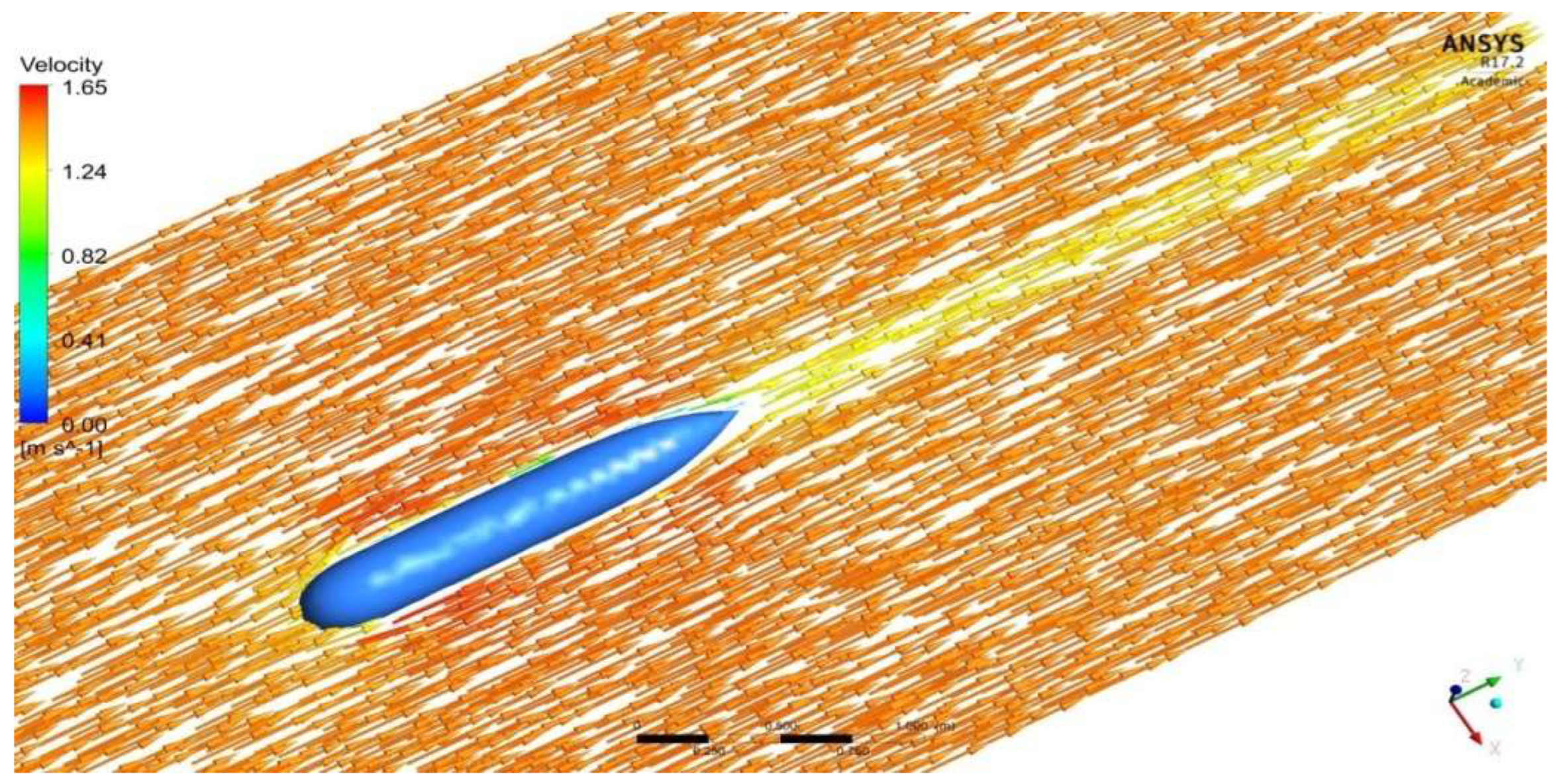
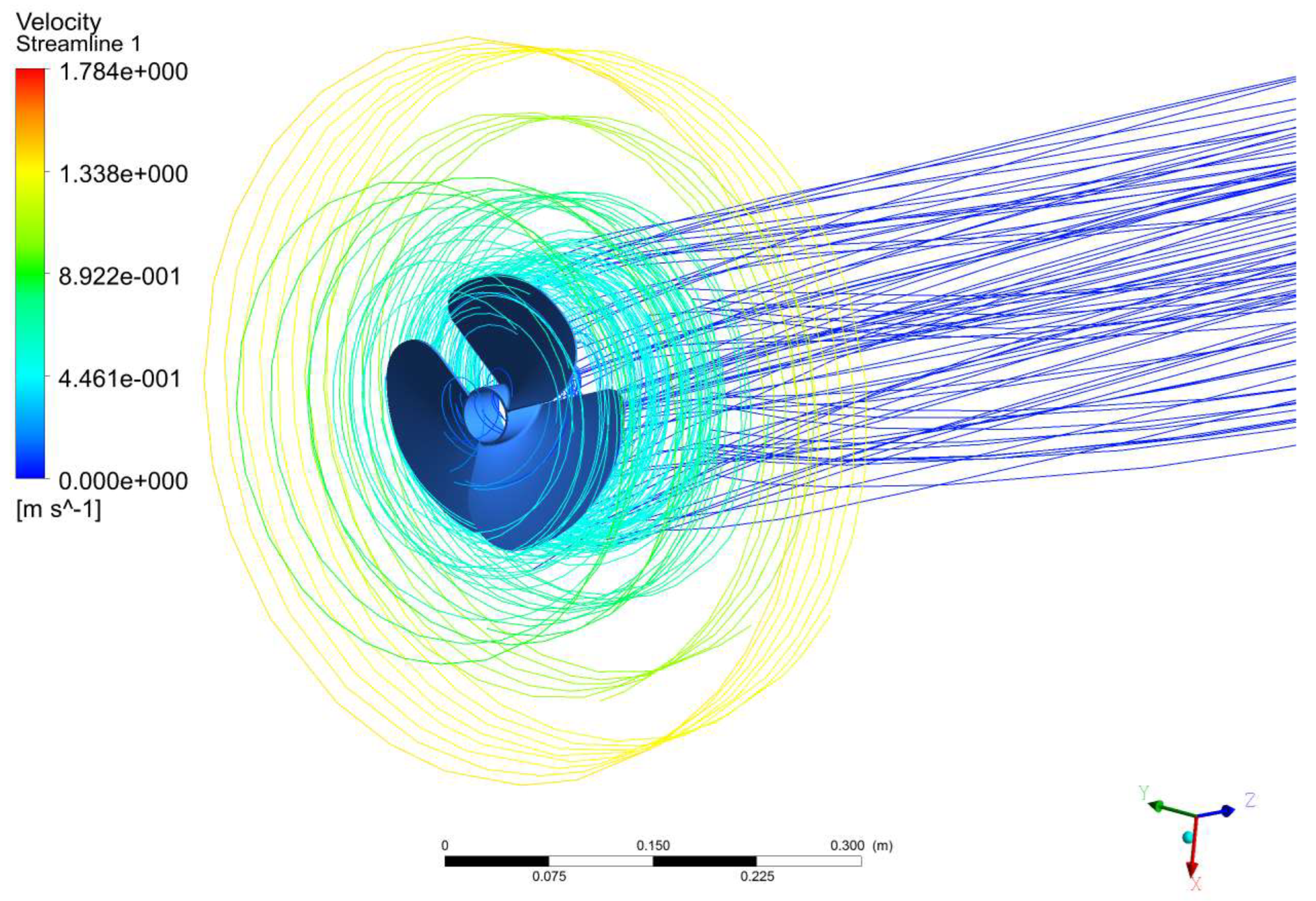
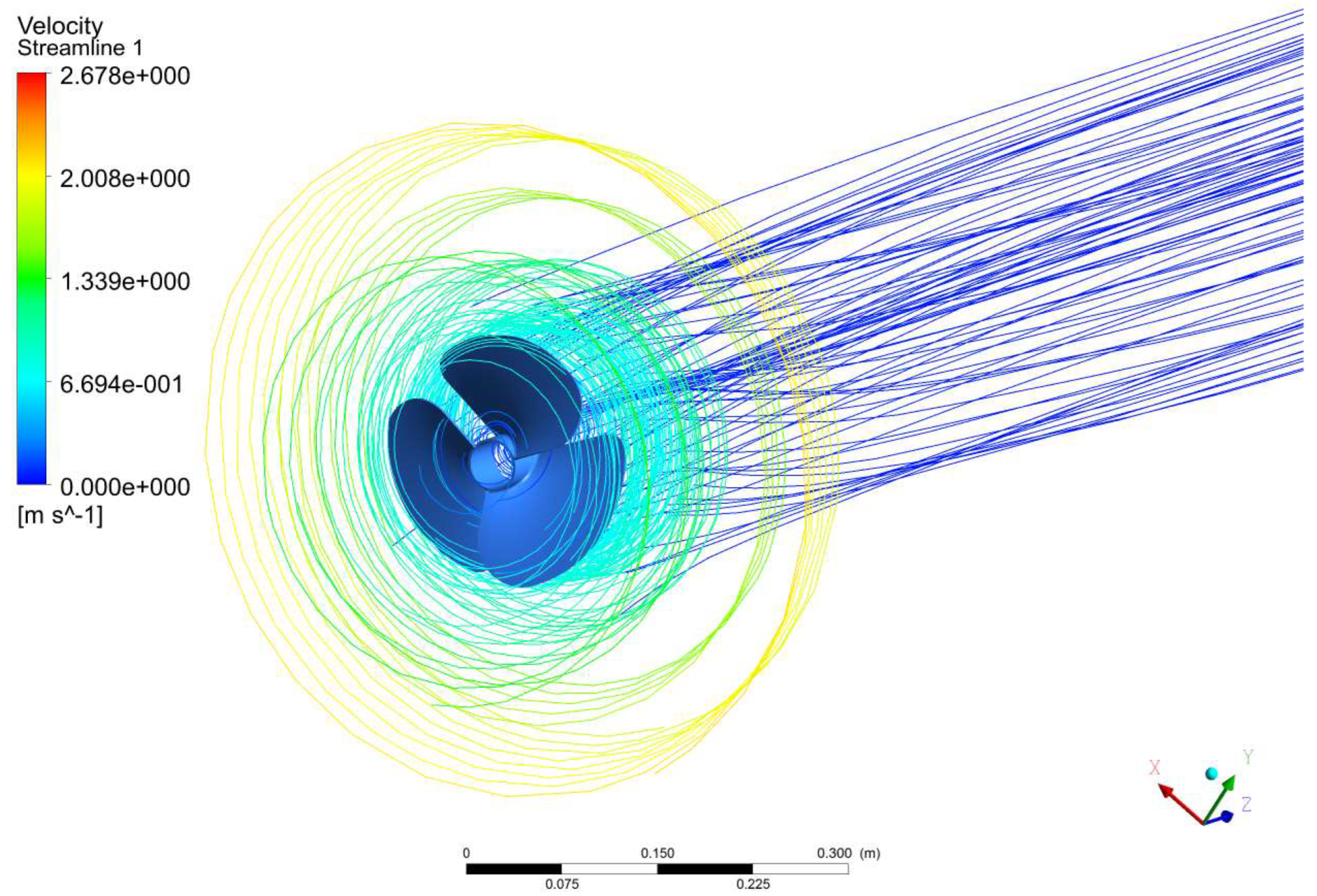
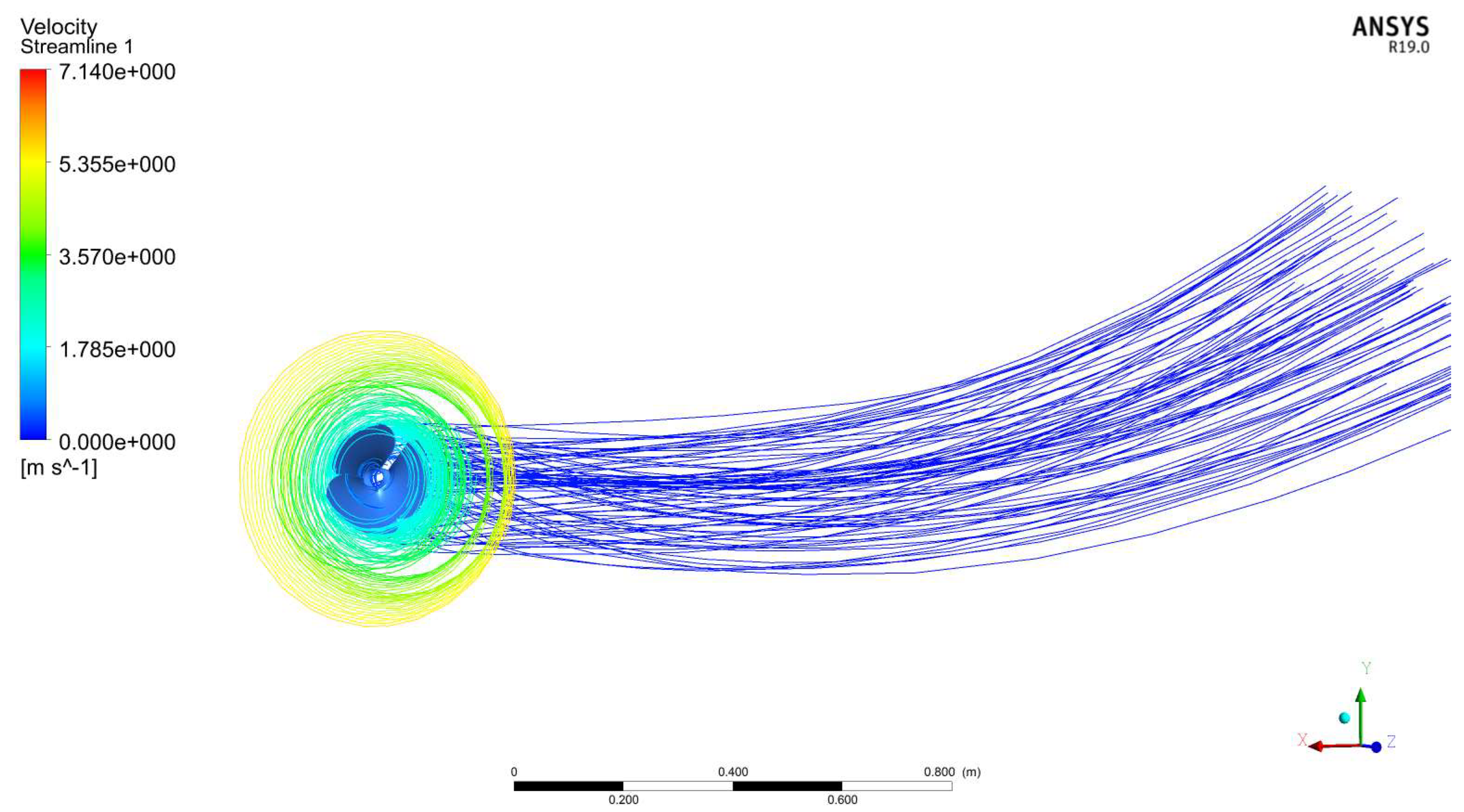
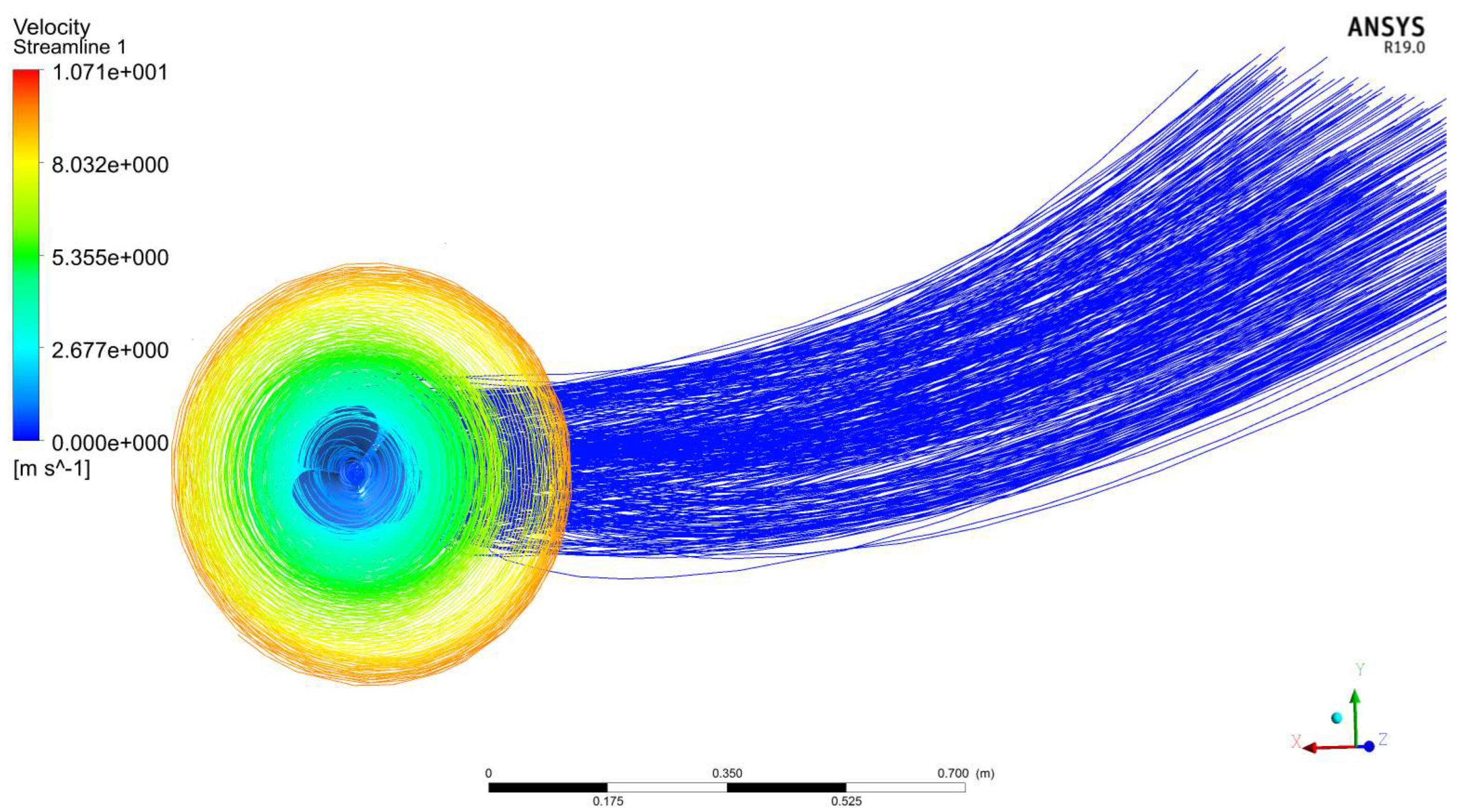
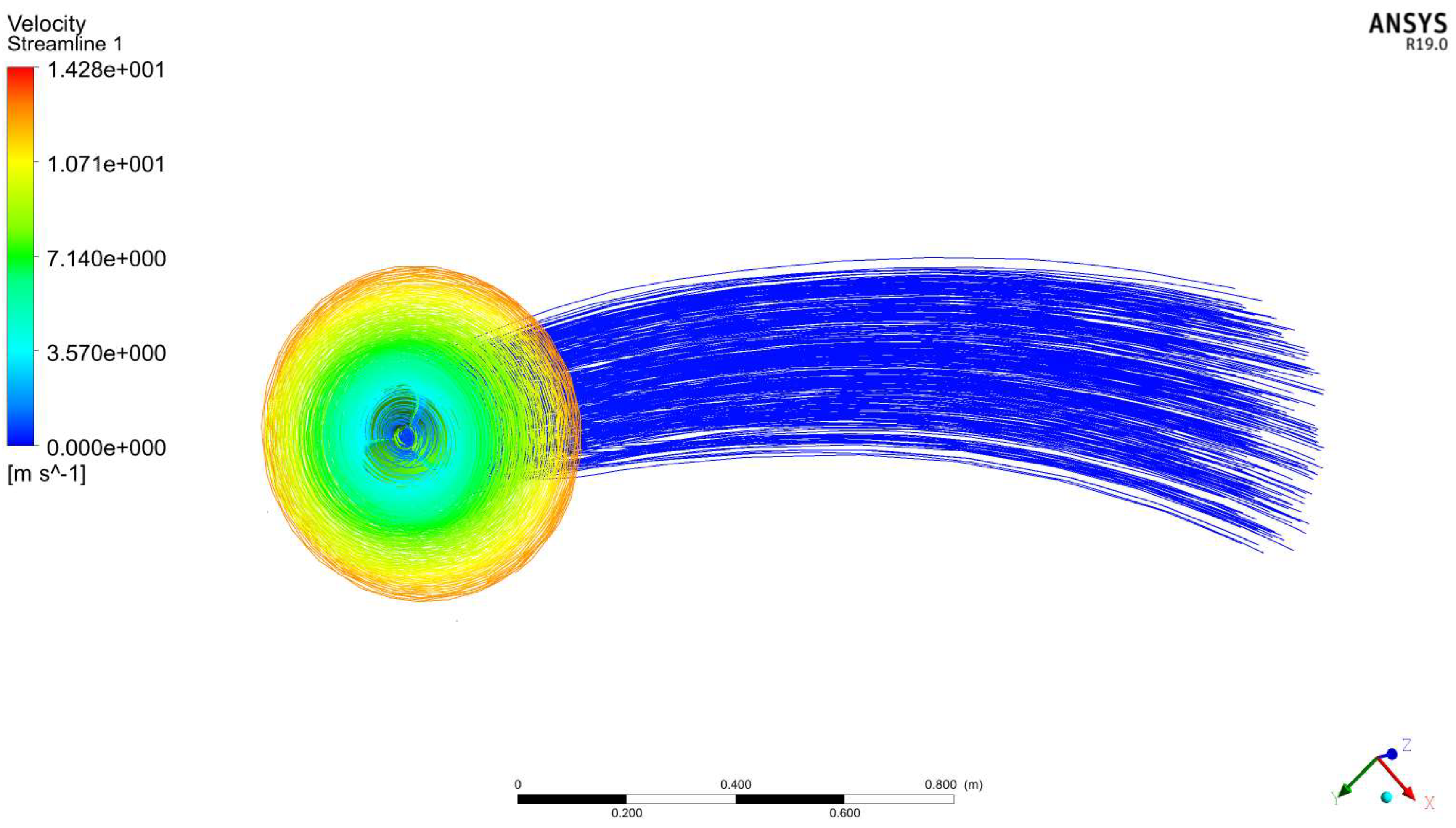
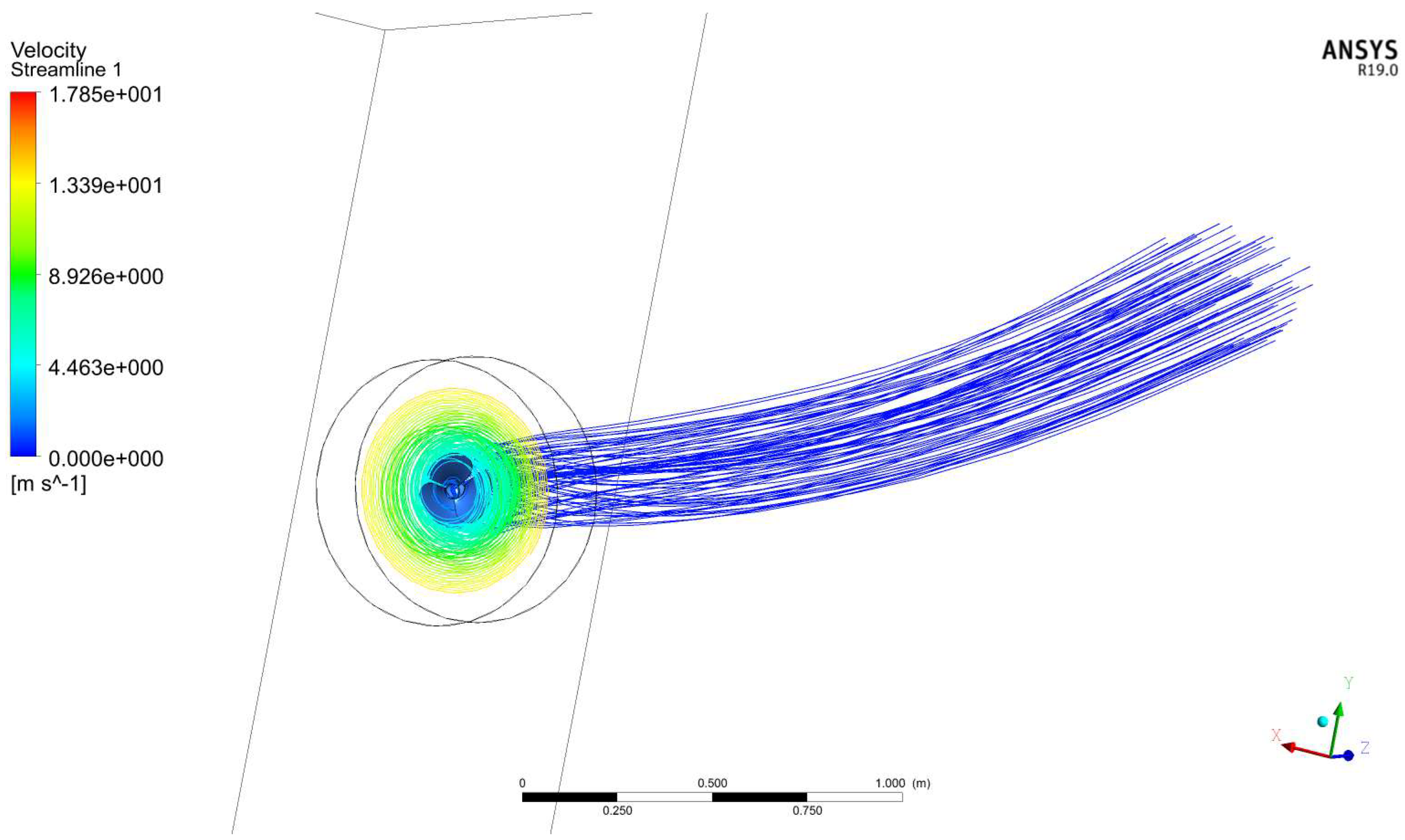
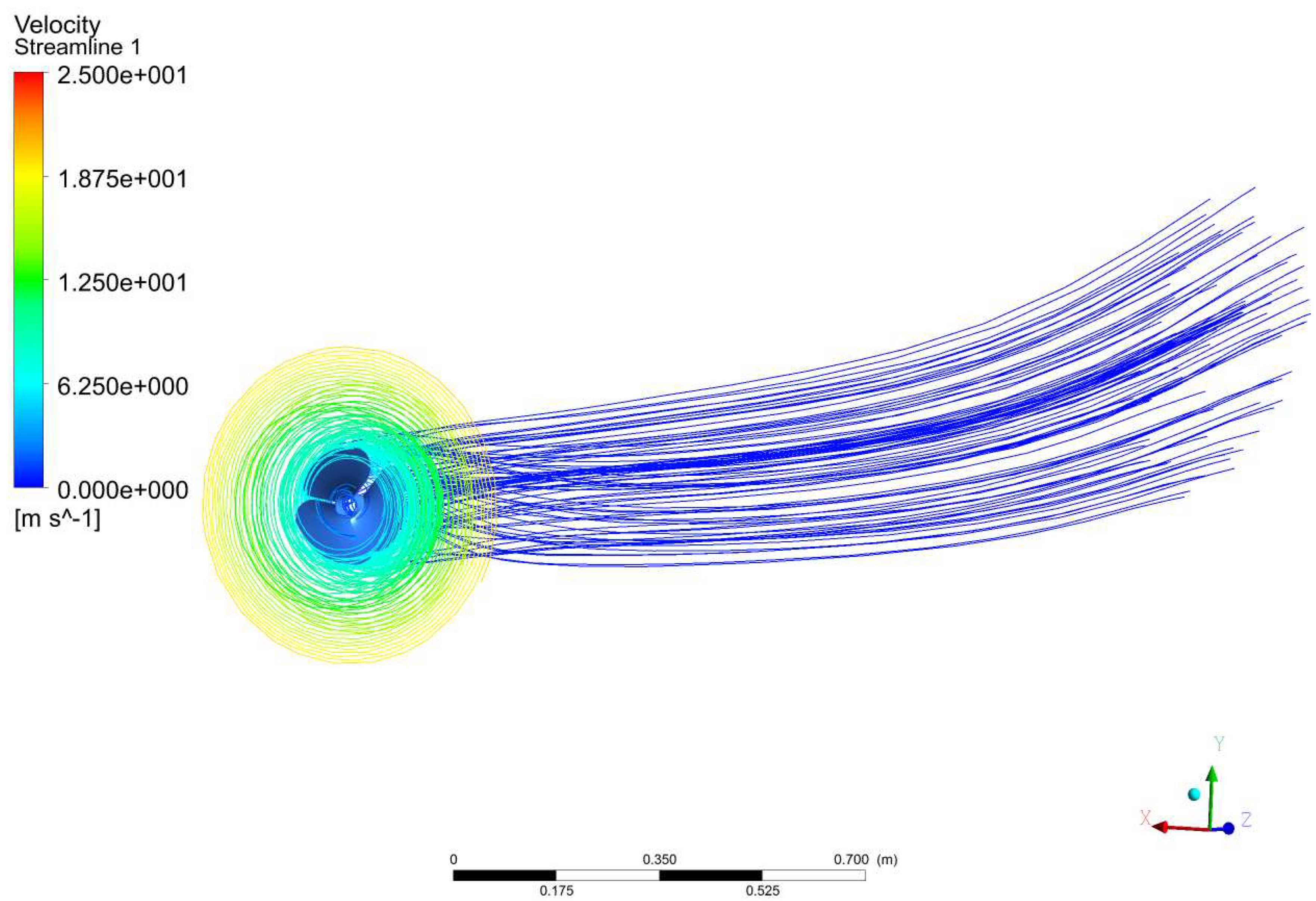
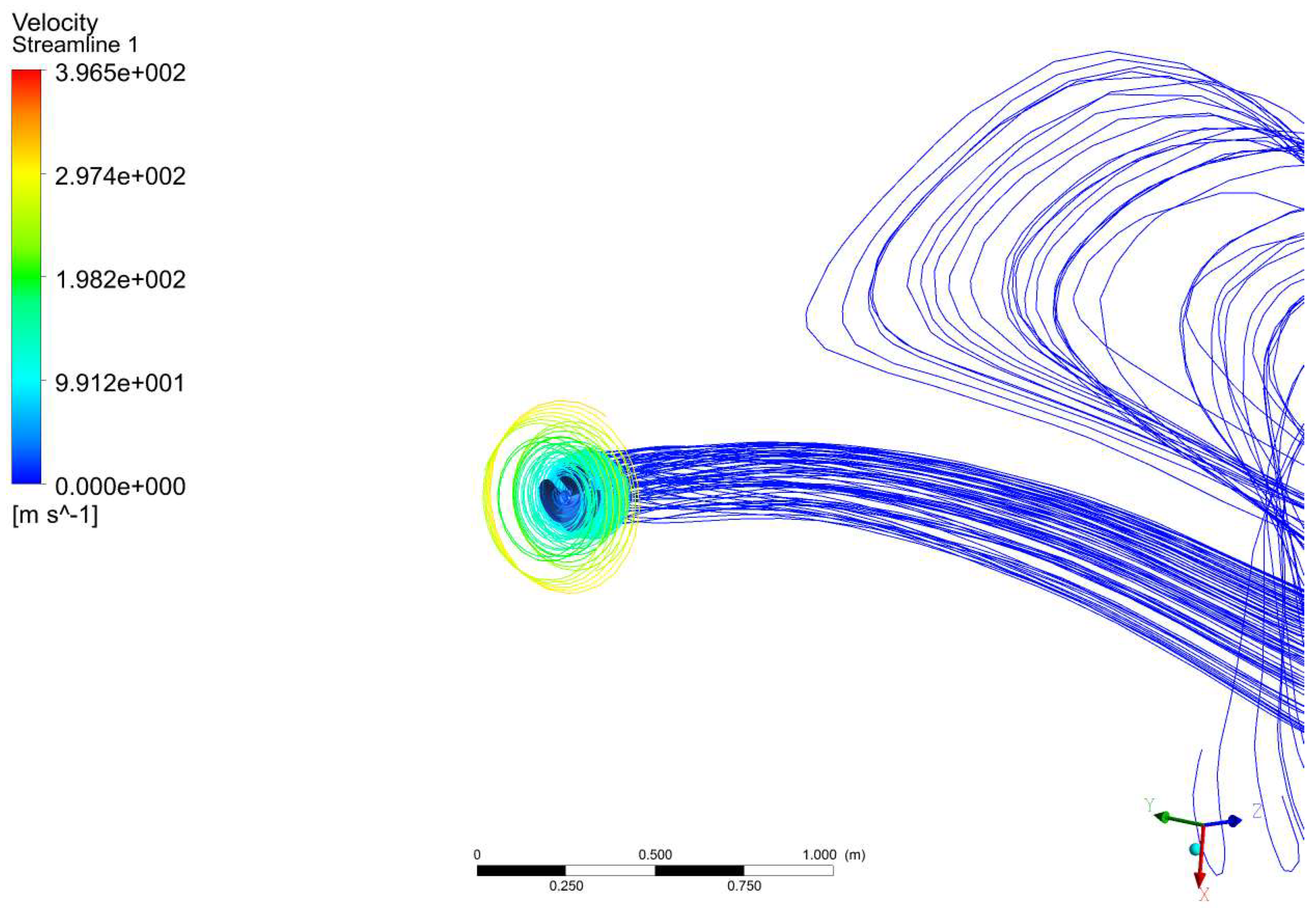
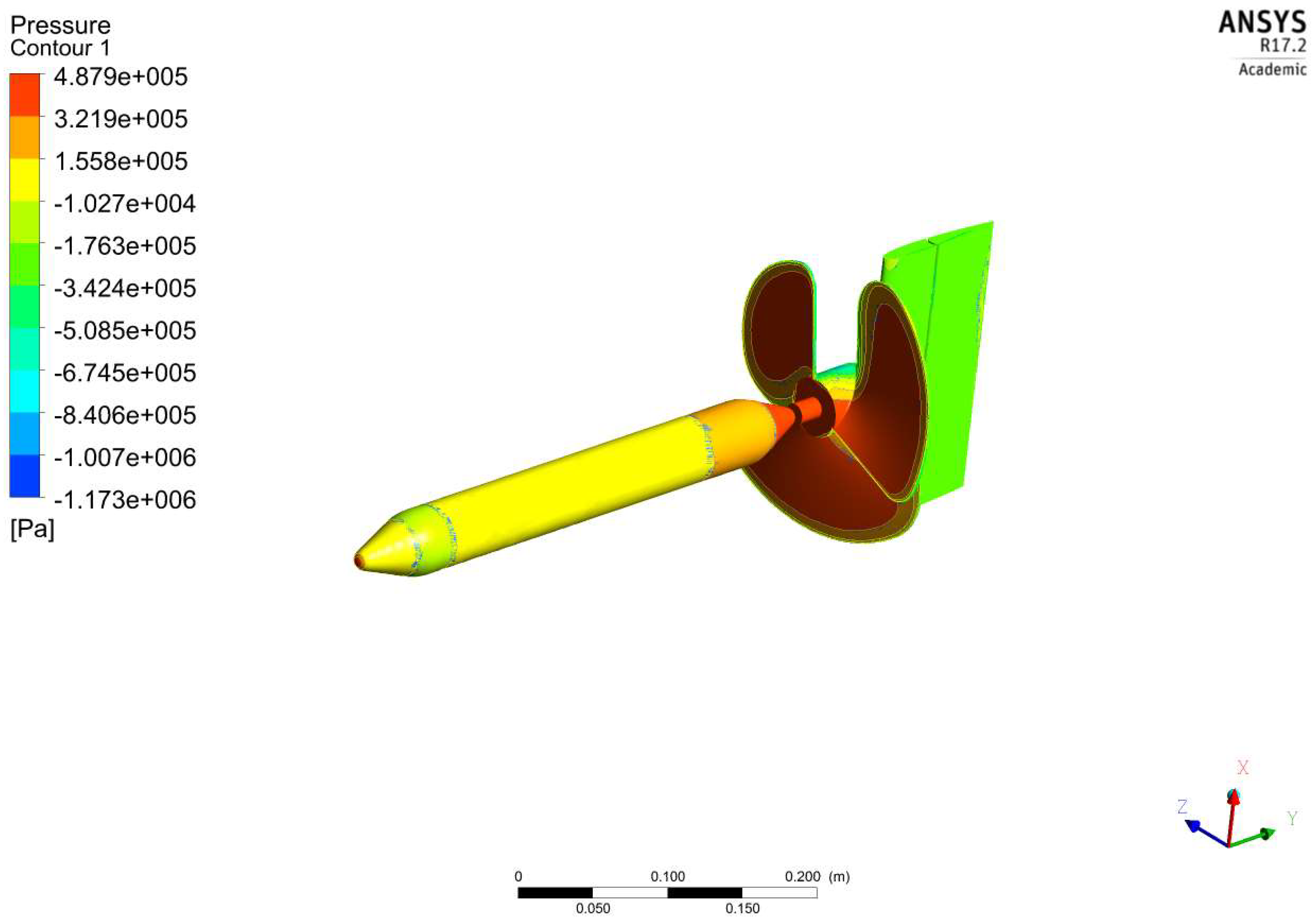
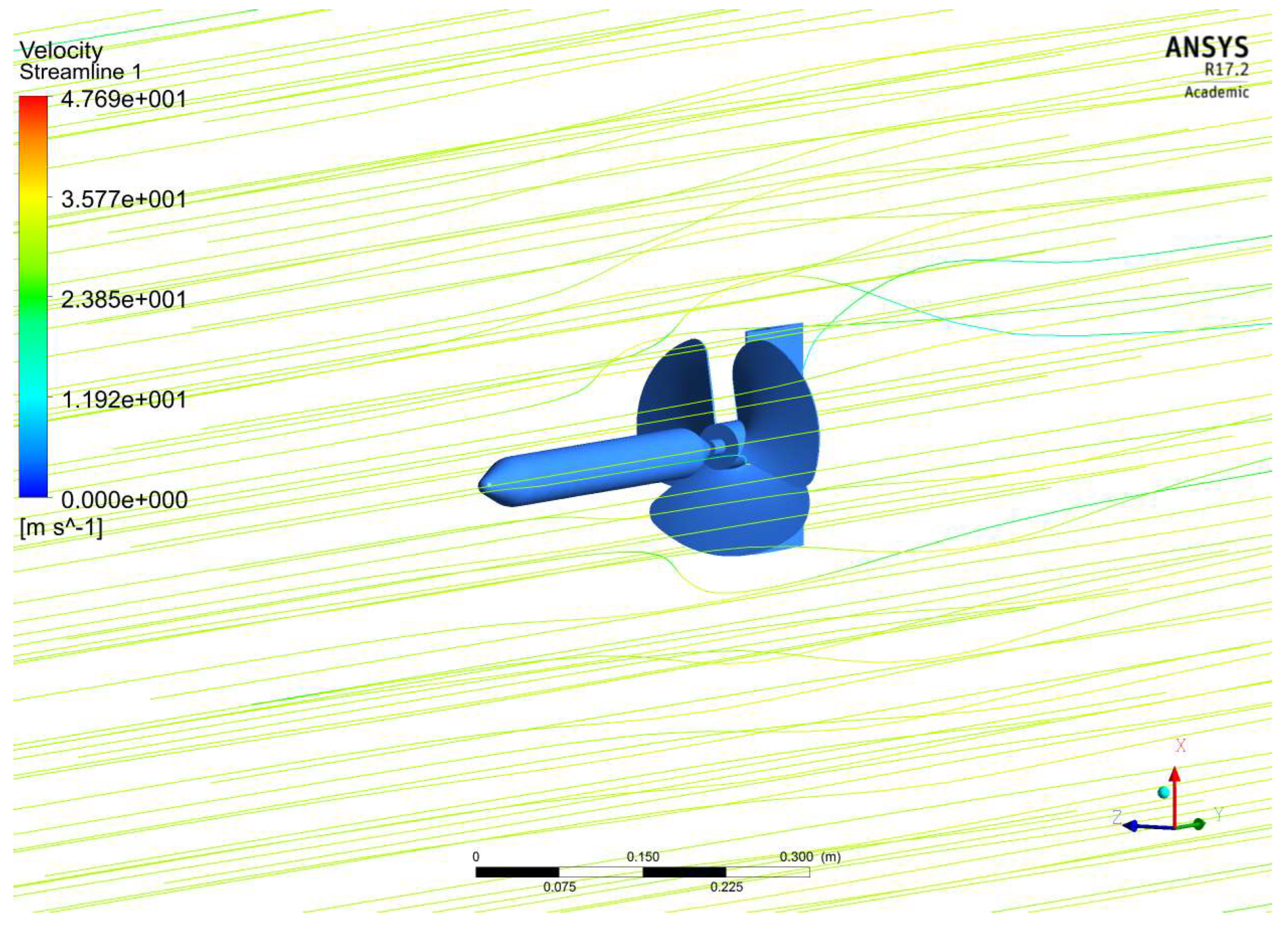
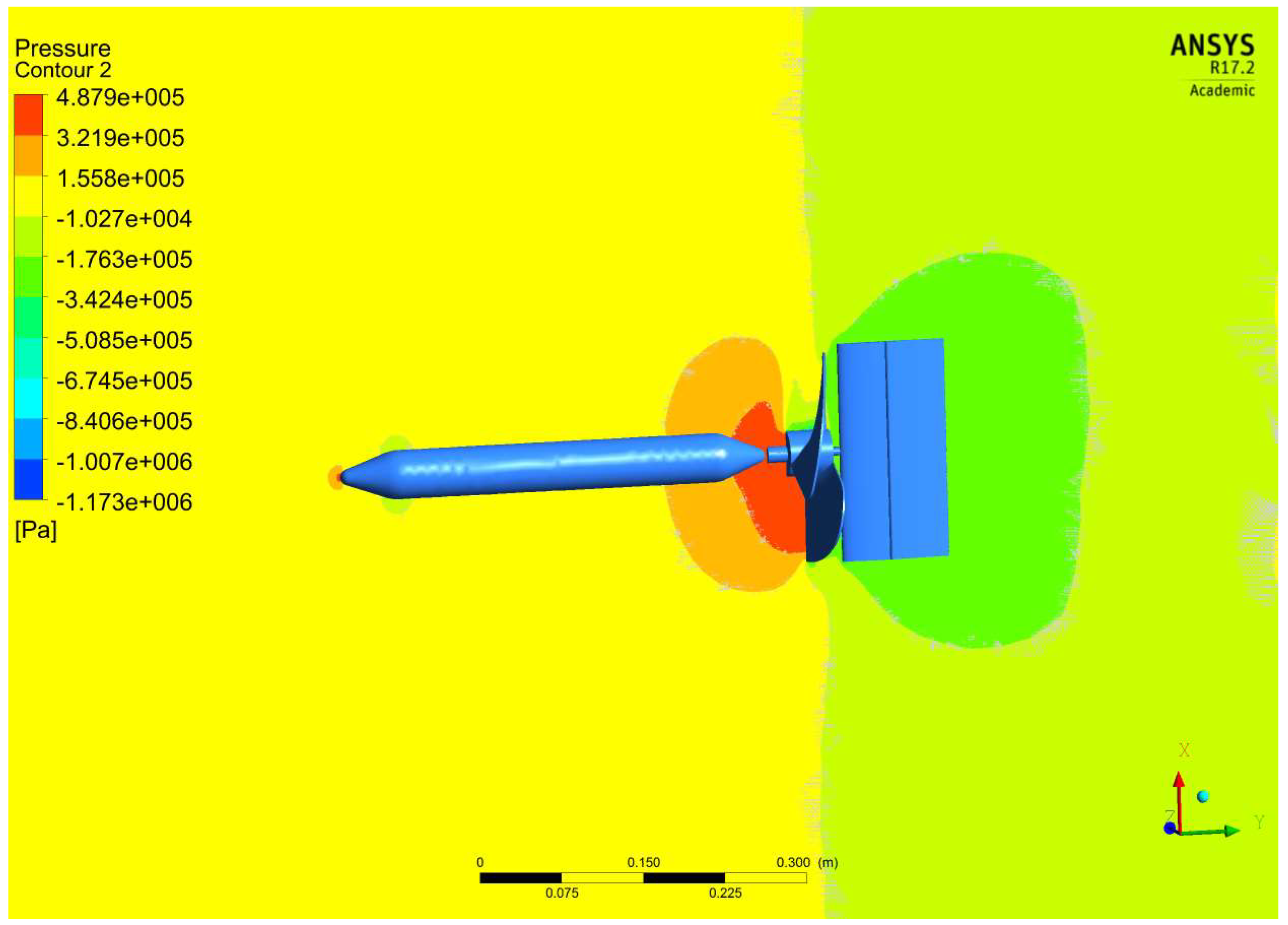
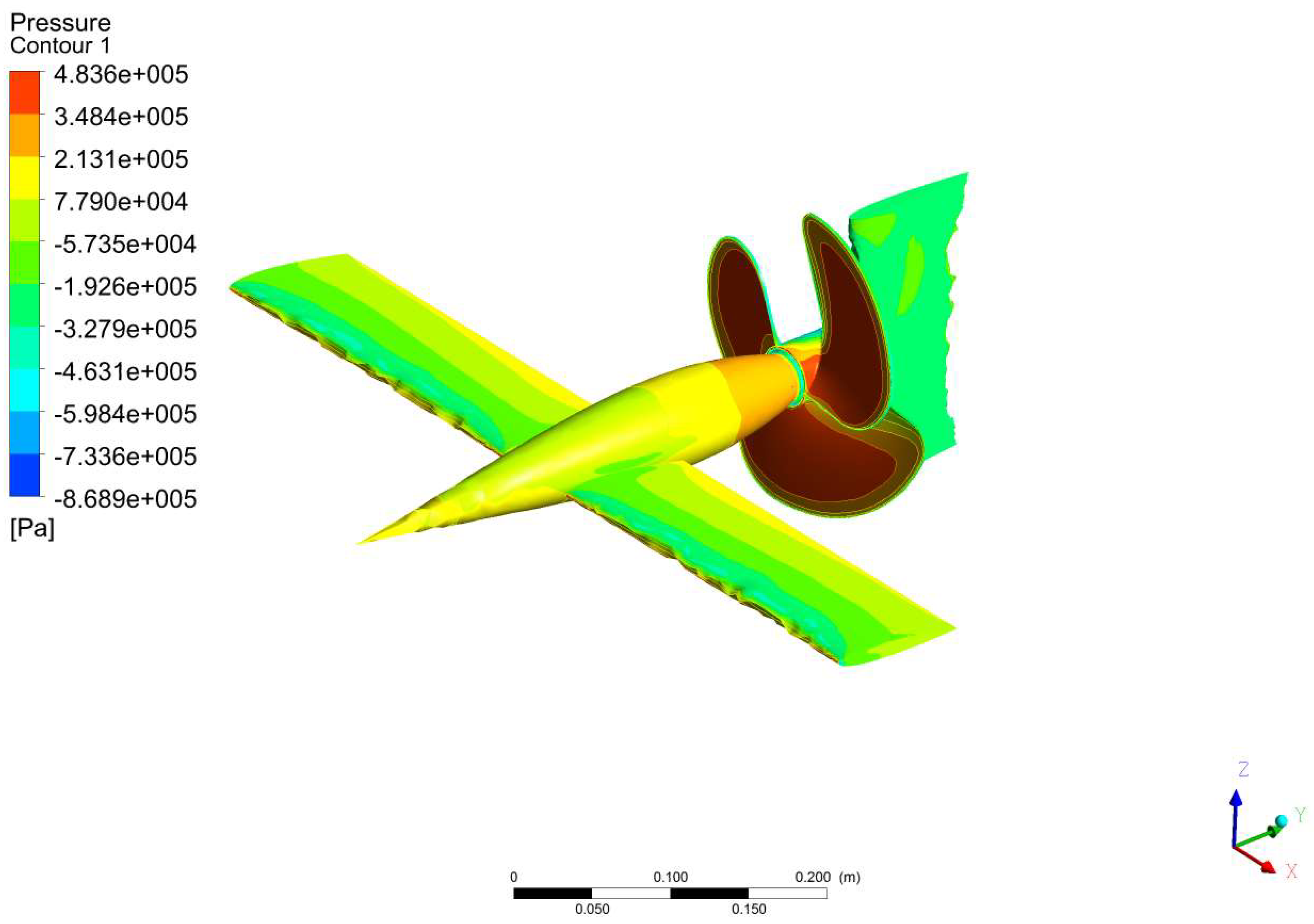
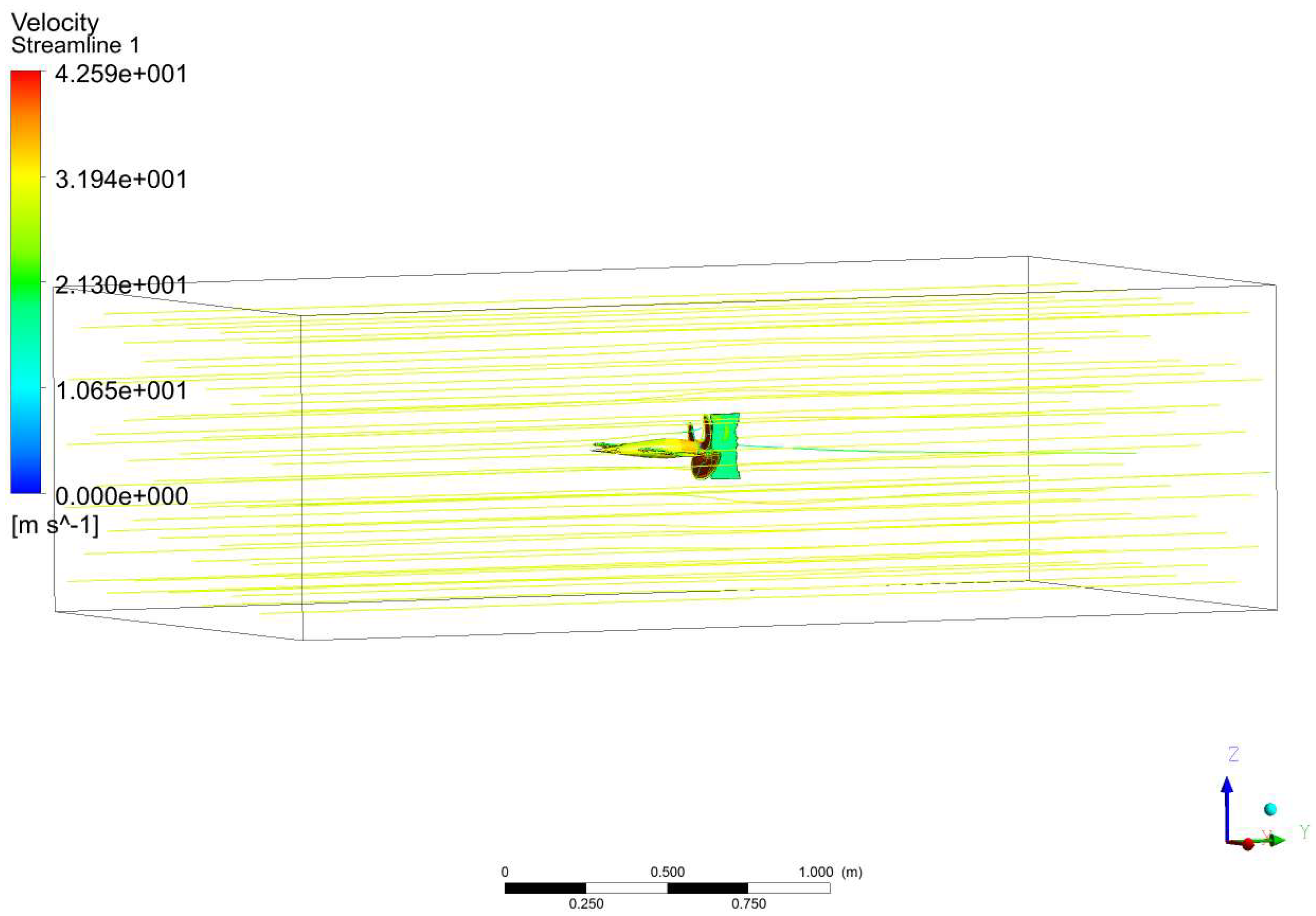
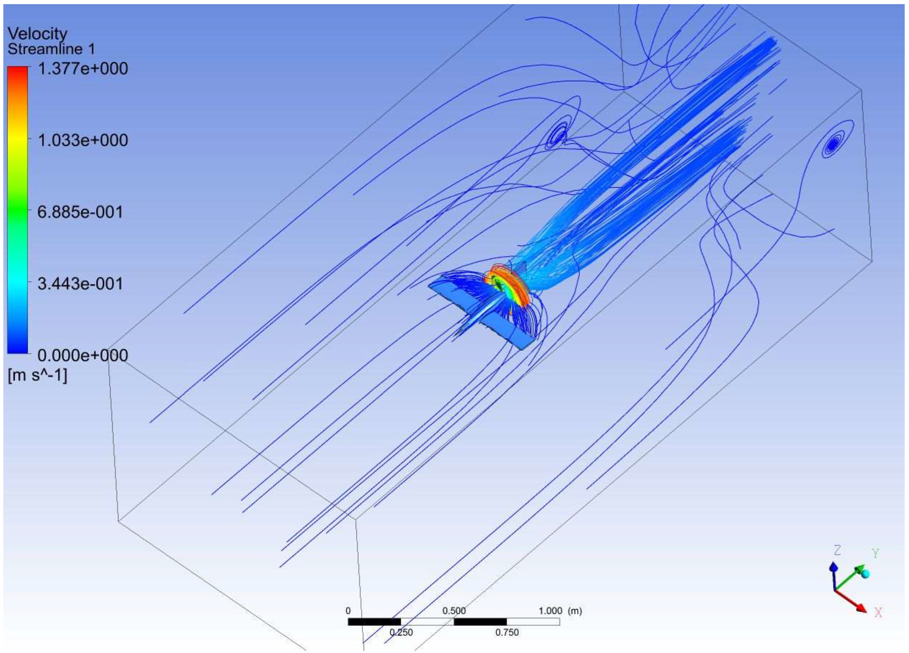
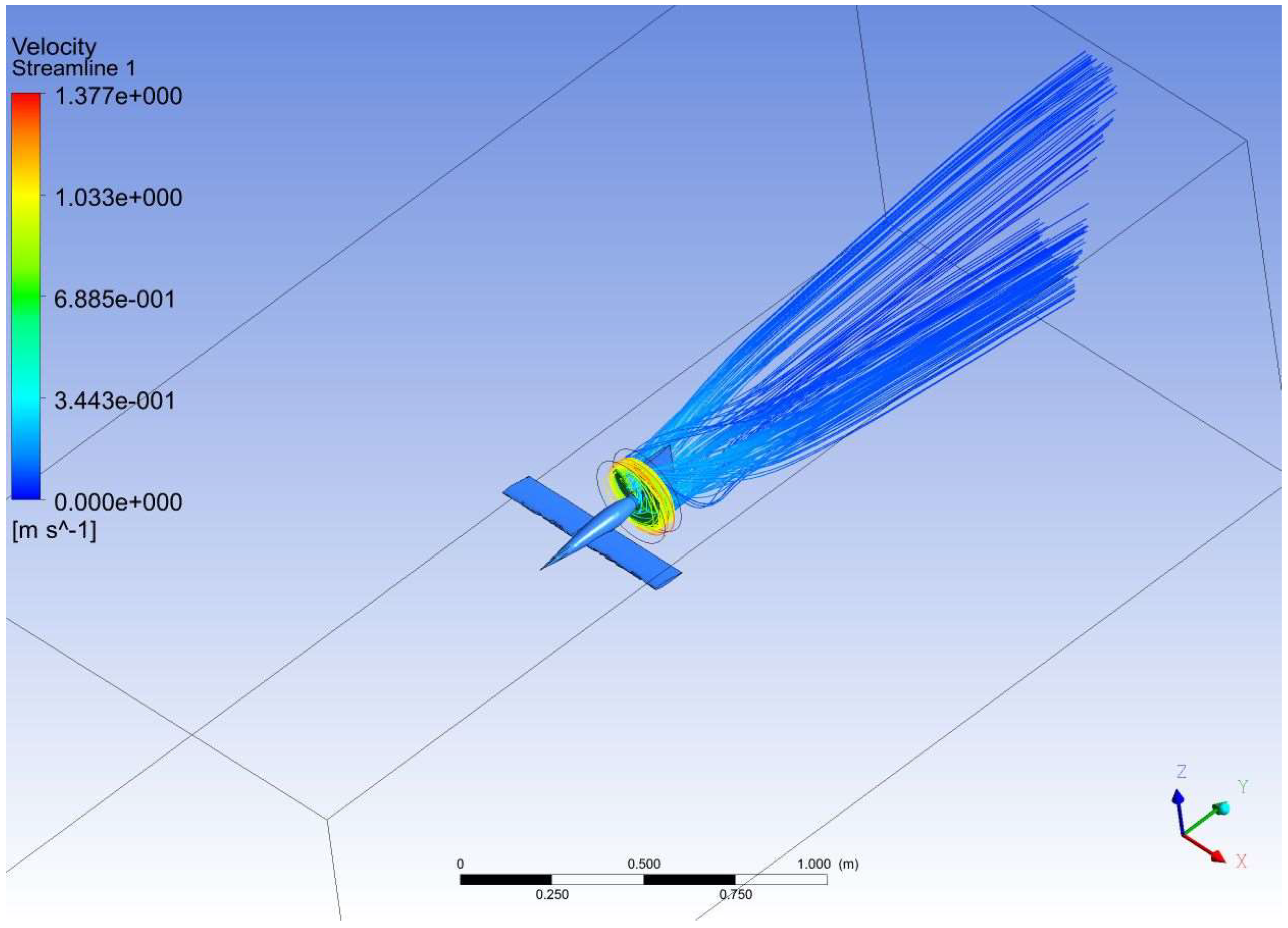
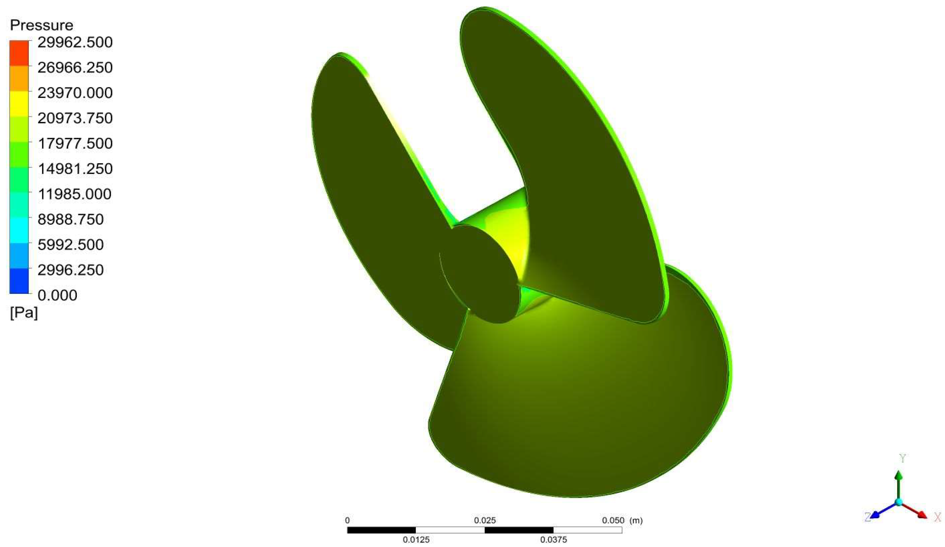
3.1. Computational Hydrodynamic Results of Propeller

With the help of relevant boundary and initial conditions, the computational simulations are computed on various US positions and the needful outcomes such as hydrodynamic &aerodynamic pressures impact on US, hydrodynamic &aerodynamic velocities in and over the US, various forces induced over the imposition of US are captured. Figure 14, Figure 15, Figure 16, Figure 17, Figure 18, Figure 19, Figure 20 and Figure 21 depict the results of dynamic cum transient evaluations performed on the US propeller for the aforementioned rotational velocities under the boundary conditions described [35,36,37,38,39,40,41,42,43,44,45,46,47].
The total thrust outputs for various RPMs of the US propeller are listed in Table 2.

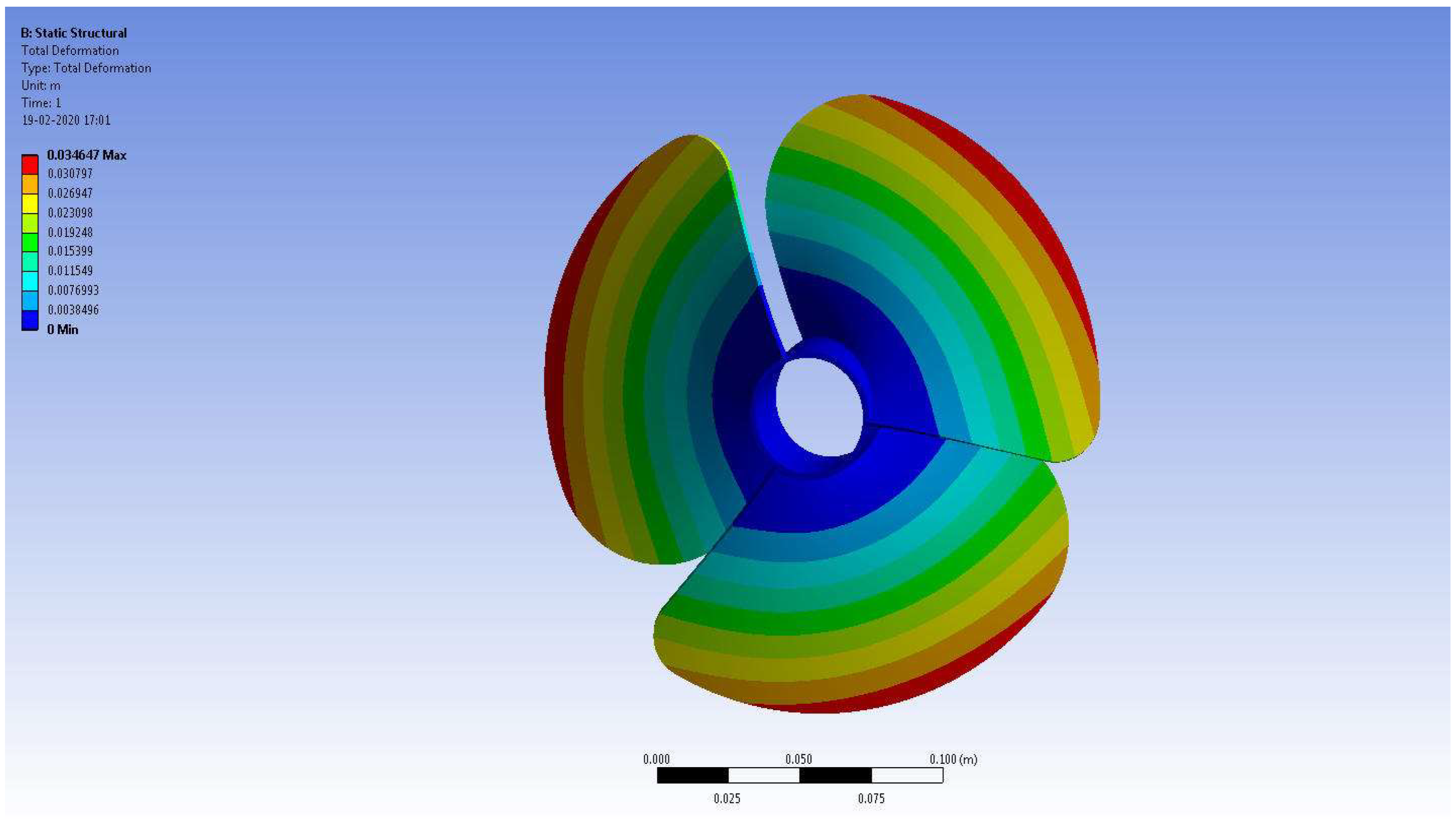
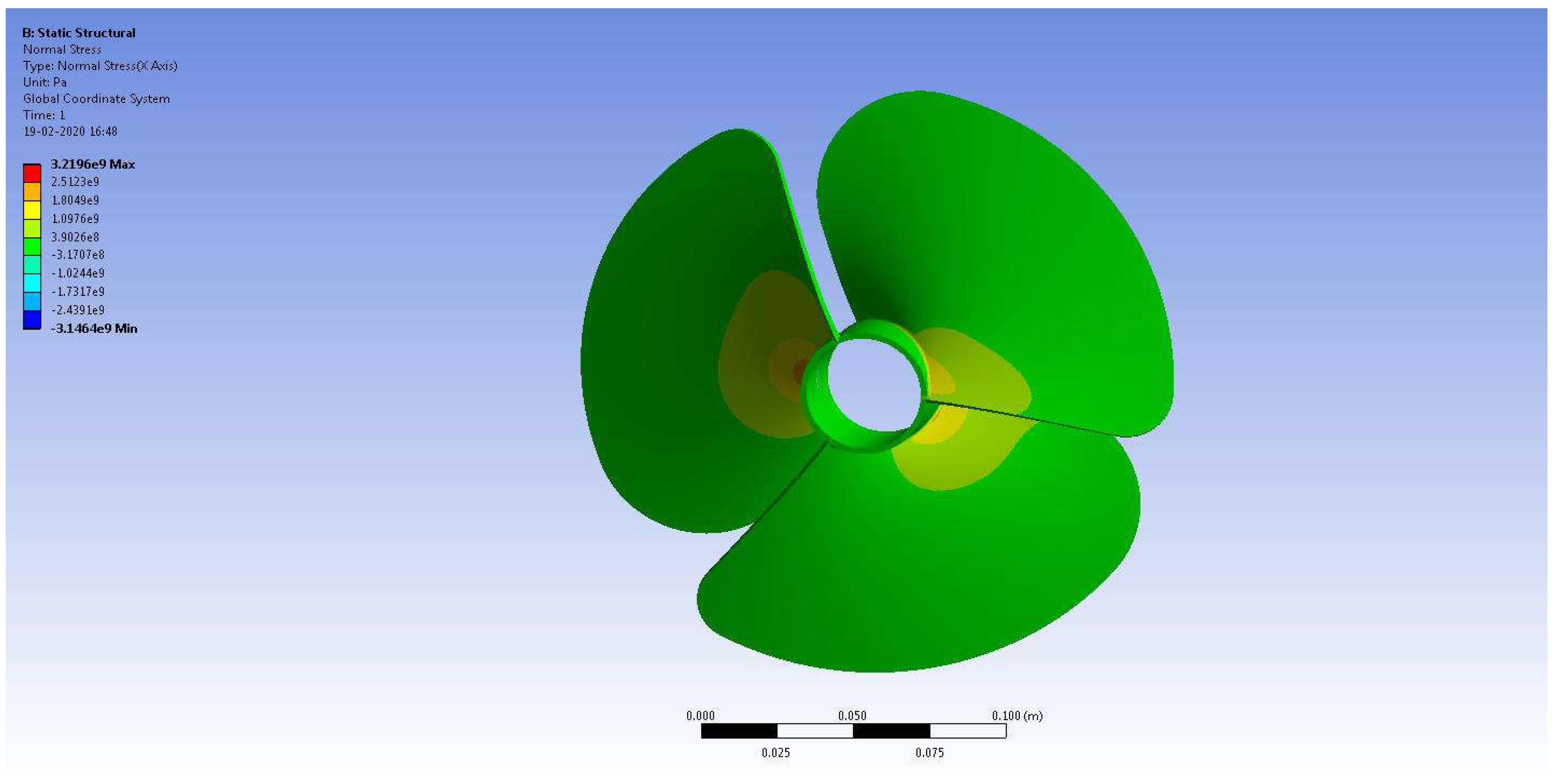
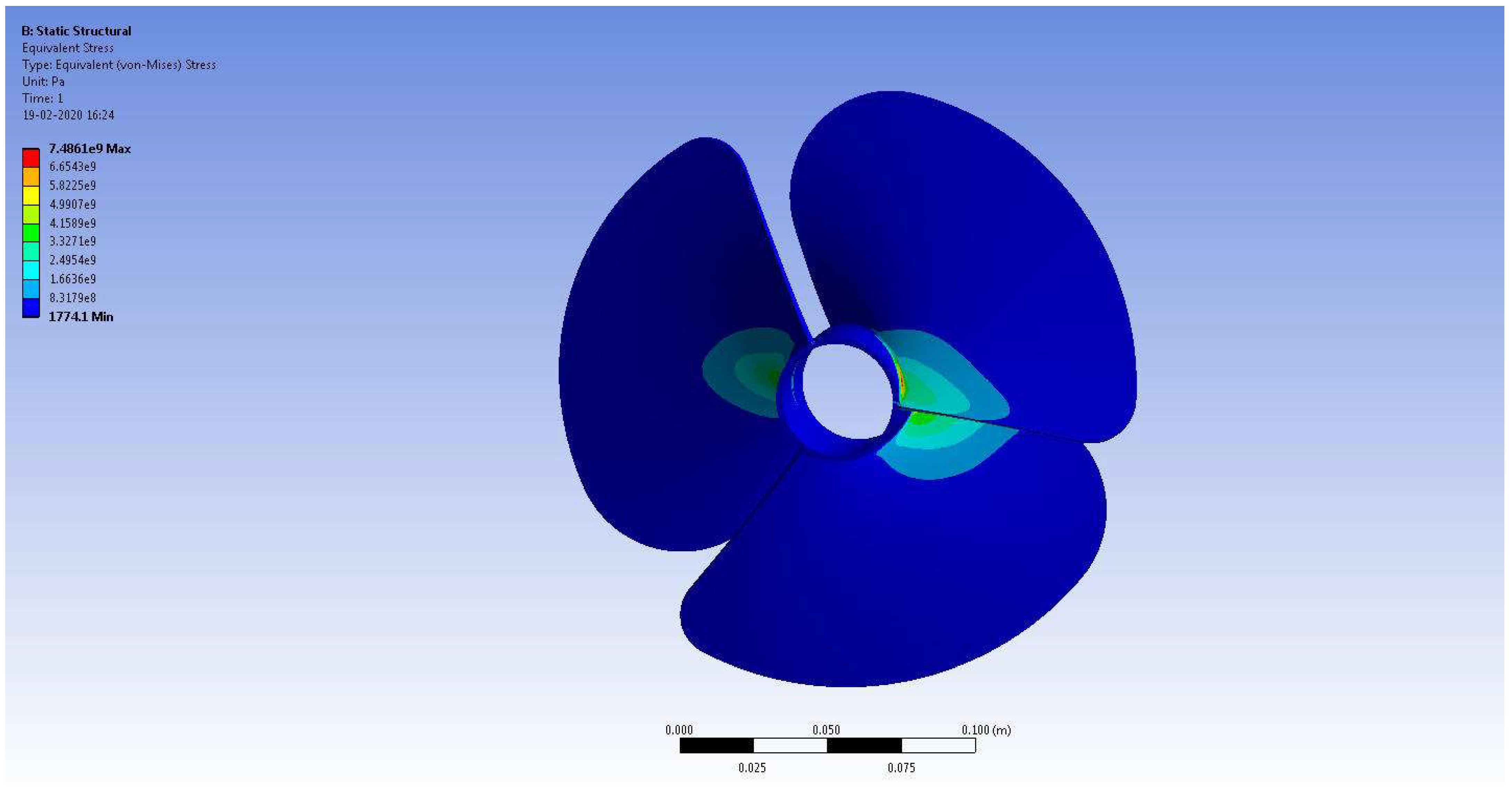
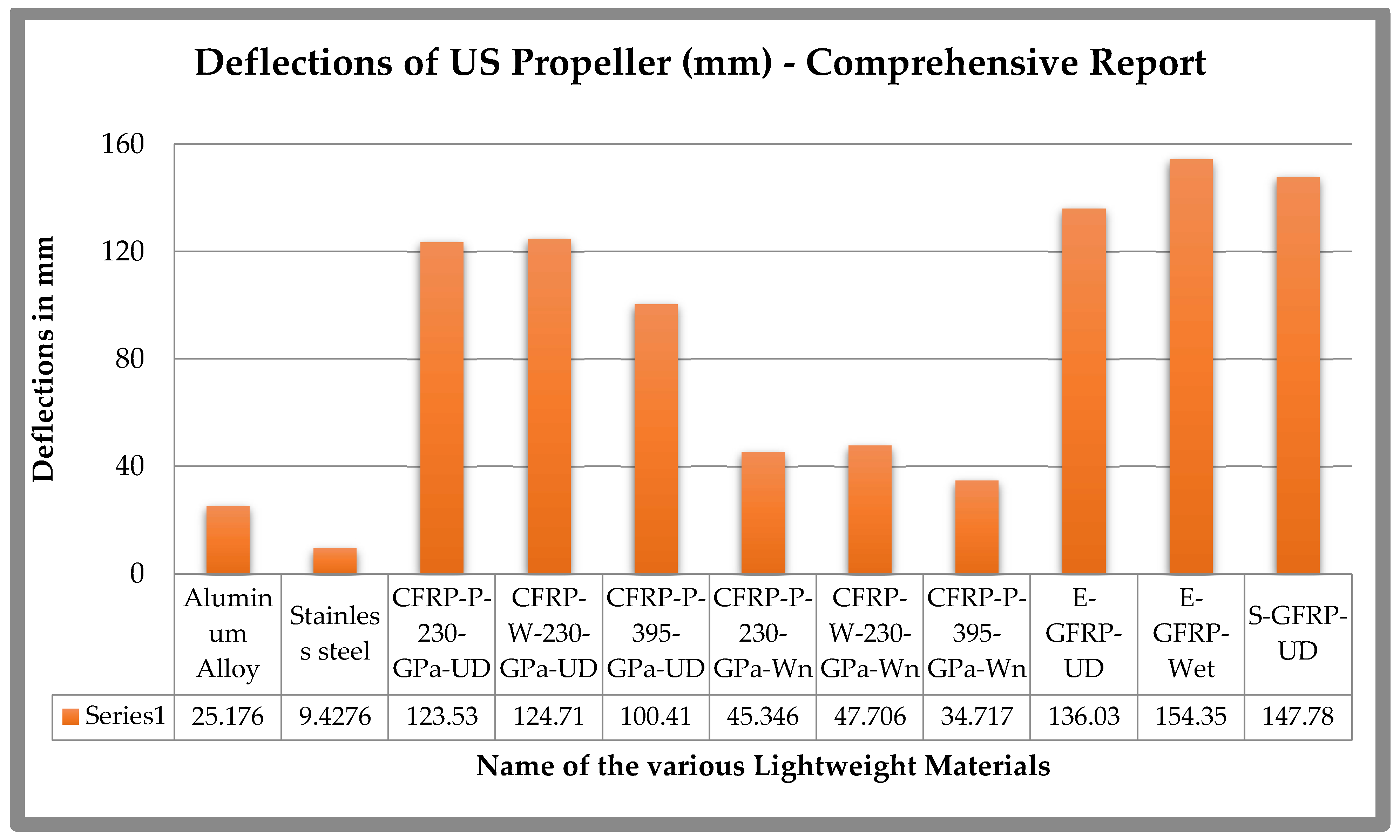
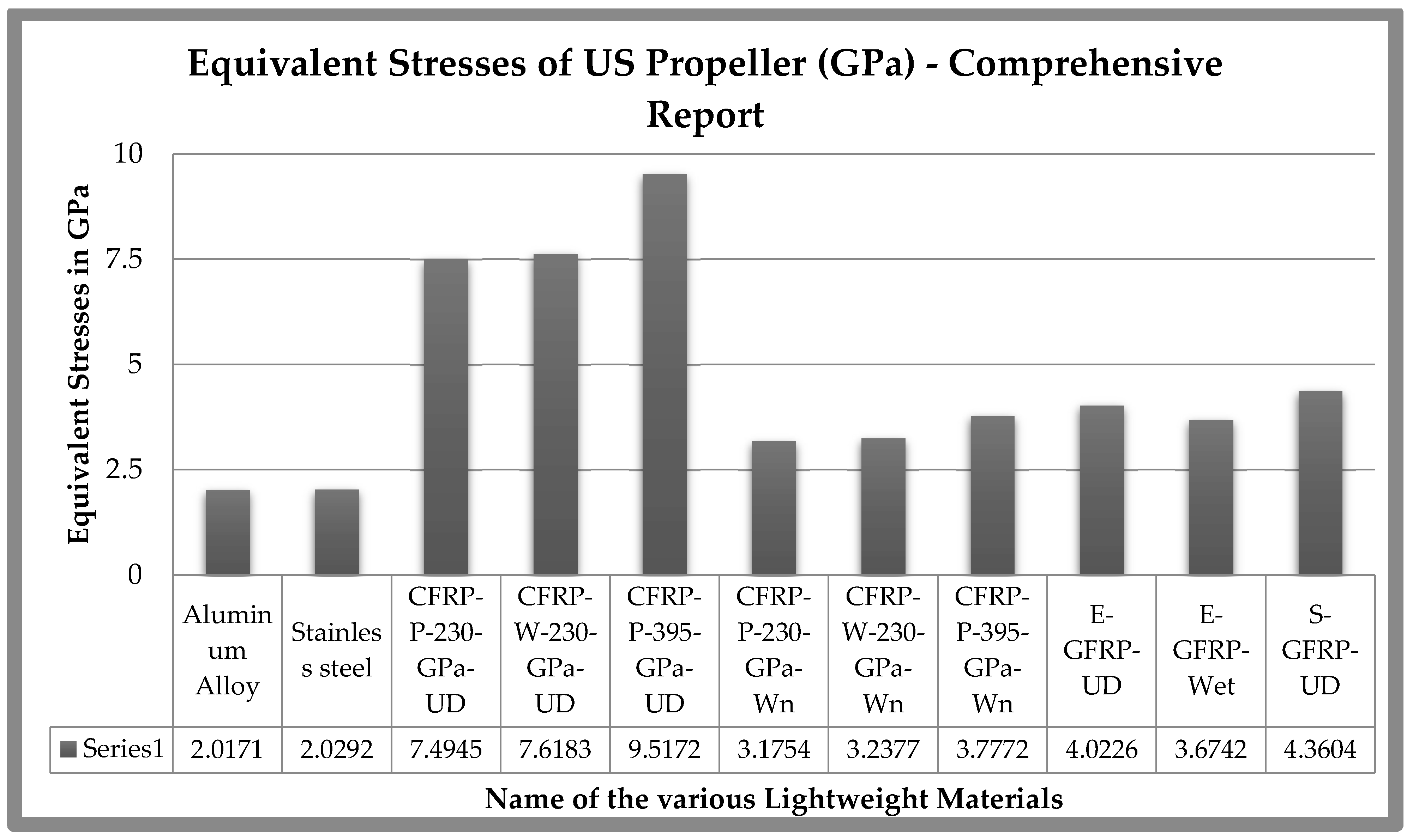
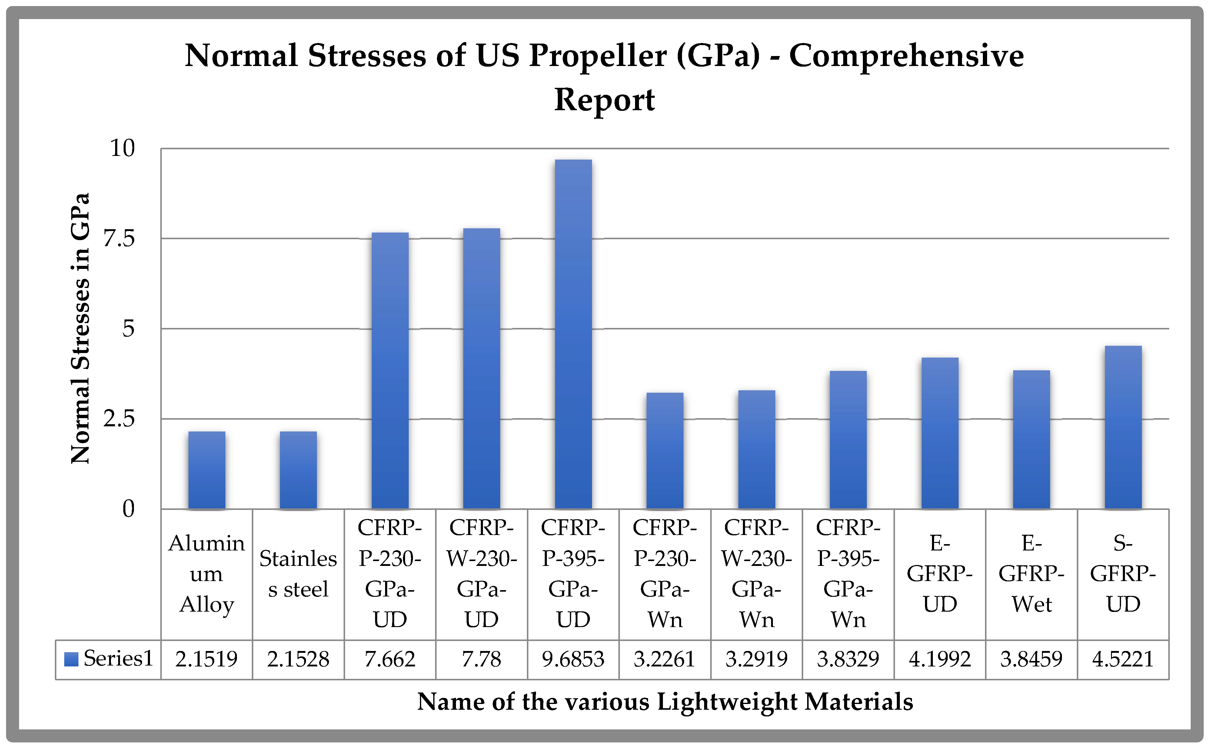
3.2. Material Optimization for the US

The watercraft model’s mass and weight are adjusted to account for the use of different materials in the US. Support for choosing the Propeller’s RPM about total US weight for different materials is listed in Table 2 and Table 3. For instance, if a propeller made from carbon woven wet can generate 29 N of thrust at just 25 RPM, it would be possible to reduce the power necessary for propeller operation significantly. However, in the case of other current materials, the RPM is rather high. This requirement for high RPM can potentially cause mechanical failure in the US, despite using tried-and-true components such as stainless steel and aluminium alloy.
The water’s hydrodynamic behaviour is accurately modelled by the pressure-based solver, which is used here. Since the hydro fluid is naturally dense, the turbulence formulation probability is smaller than other fluids; consequently, the first-order k-epsilon turbulence model is necessary for this investigation. Water being the chosen fluid, the original density requirement of 1025 kg/m3 has been adjusted accordingly. For altitudes of 0.1 m and 300 m, operating pressures of 102,330.525 Pa and 3,117,900 Pa, respectively, are used. The mission’s operating depth, the water’s density, the force of gravity, and the ambient cum air pressure have all been factored in thoroughly during the calculating stage. For both scenarios, it is usual practice to utilize the velocity inlet-based computation, where the fluid velocity is assumed to be 20 m/s from the outset. The authors know the pressure release of 0 Pa at the outlet through boundary conditions. While the control volume wall is given a low friction behaviour based on a free slip, the hydro propeller is given a high friction behaviour based on no slip. The pressure-velocity coupling based attempt has been used in this investigation through SIMPLE scheme, and the continuity and momentum equations are all of the second-order variety. All HIS analyses include the boundary mentioned above conditions and numerical recording graphs. The results of a structural analysis of CFRP-based polymer matrix composites (PMCs) are illustrated in Figure 22, Figure 23 and Figure 24.
The HIS study has been performed on the most important lightweight materials. Two materials are chosen in the alloys family since they are the most common in this field and enforced, while nine materials are chosen and imposed in the composites family. The CFRP composite is the top performer because of its long service life and superior stiffness properties. The integrative effect of low weight, long life, and rigidity was used to make this decision. Therefore, CFRP is a better choice than lightweight alloys for achieving the aforementioned integrative effects. Furthermore, the PMC made of CFRP-Prepreg-230-GPa-Wn is suitable for low-level depth and can withstand a high hydrodynamic load. The findings of a structural investigation of a carbon-woven-wet-based PMC are depicted in Figure 22, Figure 23 and Figure 24.
Comprehensive hydro-structural results for US propellers in high-depth level working settings are revealed in Figure 25, Figure 26 and Figure 27. In this complex simulation, the same 11lightweight materials—two of which are alloys, six of which are CFRP-based composites, and three of which are GFRP-based composites—are put through their paces. The main goal of this detailed simulation with a high-depth orientation is to assess further the resilience of the top performers from a low-depth level instance. The authors concluded that the chosen material could withstand hydro structural loads from both situations [51,52,53,54,55,56,57].
Other than the major alloys and the CFRP-woven-prepreg-based PMC, the CFRP-woven-wet-based PMC responded with quite low structural effects at the high depth of the hydrodynamic environment. Therefore, these materials are the best performers for high-level depth-based real-time applications.

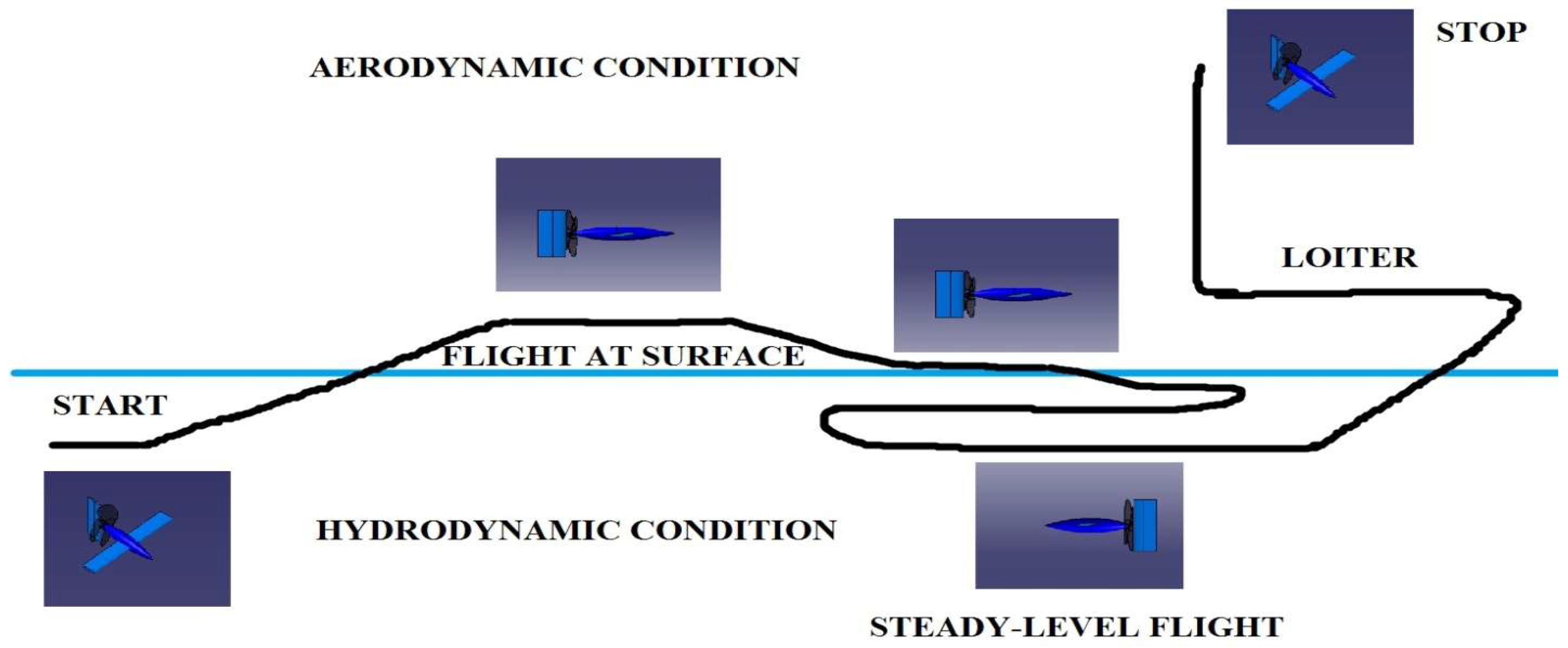
3.3. Results of US at Steady Level Flight

The exterior shell, rudder, control surface, and propeller speed are all examined using SMRF analysis. First, a preliminary model of the underwater UAV is developed in CATIA and then analysed with ANSYS Fluent [16,17,18,19,20]. Next, CATIA is used to create a spline-based model of the second US, which is then shaped into an extremely aerodynamic form. Finally, drag caused by the body, the pressure surrounding it, and velocity streamlines are extracted from the models after being imported into ANSYS Fluent for flow analysis [26,27,28,29,30]. The aforementioned computational outcomes are typically revealed in Figure 28, Figure 29 and Figure 30 for further clarification [30,31,32,33,34,35,36,37].

3.4. Results of US at Climb in and on the Water Surface

The streamlined fuselage for model two is designed using spline, which has a smooth curvature at the end of the fuselage and a tapered front portion similar to fish. Since the body must accommodate the necessary components, the length is maintained at 43.5 cm, and the maximum diameter is enhanced in the posterior part of the fuselage. With an 87 cm wingspan, the same propeller, and the Becker rudder, a control surface similar to an aileron is fixed for latitude stability. Since the main requirement is manoeuvrability rather than lift, the control surface is made of NACA 0012 aerofoil. The control surface aims to make a coordinated turn off the vehicle underwater. In ANSYS Fluent, the boundary conditions are steady, standard k-epsilon as a viscous model, water-liquid with a density of 1025 kg/m3. The model is examined at 5 m, and the pressure is provided as 151584 Pa. The inlet velocity is set to 30 m/s for analysis purposes. Figure 31, Figure 32 and Figure 33 depict the pressure on the body, drag force and velocity streamline, and pressure over the body.

3.5. Execution of Pitching and Yawing Manuverings through Additional Control Surfaces

The mission profile picture (Figure 1) shows that one of the manoeuvrings involved in this planned mission is altitude increment, so this phase needs to be investigated to acquire a view of the reaction of the US to this particular phase. In this regard, the unique US, along with an extended horizontal stabilizer, has been developed and imposed CHA simulations. As a result, the assumed minimum altitude increment rate is 5 m/s, and the maximum altitude increment rate is 30 m/s. Here, state-of-the-art US simulations of hydrodynamics are performed, as shown in Figure 34, Figure 35, Figure 36, Figure 37 and Figure 38.
Figure 34, Figure 35 and Figure 36 correspond to the outcomes of hydrodynamic pressure distribution and velocity variations in and over the US under maximum altitude increment rate. For high-speed manoeuvring, the hydrodynamic force on the US in the “X” direction is 762.412 [N], in the “Y” direction is 15,684.4 [N], and in the “Z” direction is −276.132 [N]. Figure 37 and Figure 38 belong to the computational hydrodynamic outcomes of the US under the condition of minimum altitude increment rate.

3.6. Deployment Test on US through CFD-SMRF Coupled Approaches—Execution State of Surveillance

The mission profile (Figure 1) shows that one of the manoeuvrings involved in this planned mission is a steady-level flight in an aerodynamic environment for surveillance applications. Therefore, in this regard, the unique US, hydro propeller, and the rectangular symmetrical wing has been modelled and also undergone the planned simulations. An underwater vehicle’s propeller is given various rotations per minute to test its responsiveness in a dynamic study. Similar to the previous study, this one uses identical boundary conditions, but this time the propeller’s rotational speed is accounted for in a transient analysis. Figure 39, Figure 40, Figure 41 and Figure 42 depict the pressure on the vehicle, the revolving propeller, and the velocity streamline between the inlet and the propeller.
The comprehensive outcomes of induced drag on both models are listed in Table 4.
Drag, manoeuvrability, and top speed are evaluated in the two versions. Finally, the proposed hybrid US is the ideal vehicle for carrying out the designated objective.

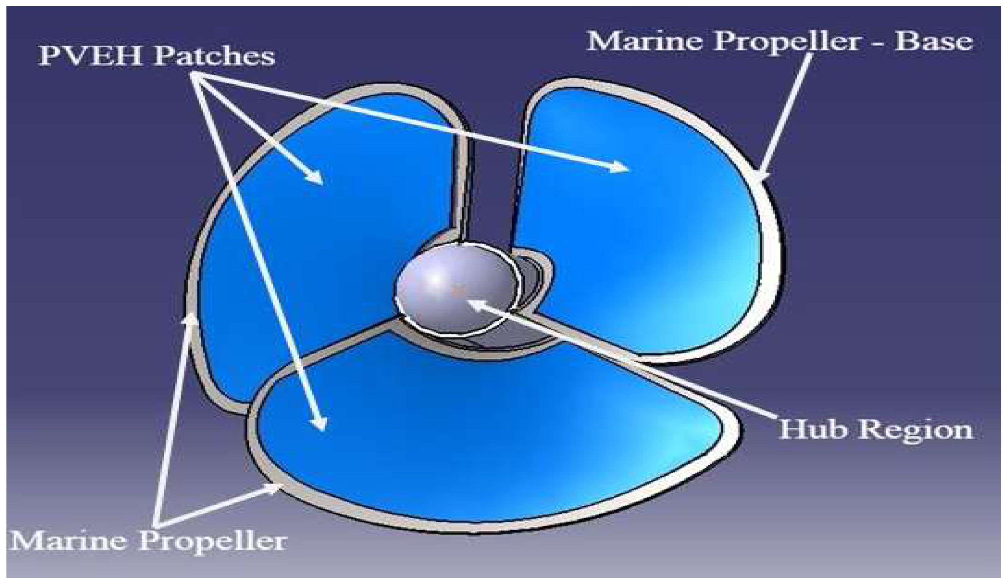
4. Self Energized Hydro Propeller for US

The CHA (computational hydrodynamic analysis) and CVA (computational vibrational analysis) are performed, and their outcomes are tracked according to the aforementioned boundary constraints. CHA and CVA have been completed using several computational approaches, such as the finite volume approach and the finite element approach. The CHA is calculated using the finite volume approach, whereas the CVA is calculated using the three-dimensional finite element method. The primary inputs for the analytical estimations of electricity generation by PVEH patches are the results of these CHA and CVA [35,36,37,38,39,40,41,42,43,44,45,46,47,48,49,50,51,52,53,54,55,56,57].

4.1. Hydrodynamic Results

Hydrodynamic results of the US propeller under normal working circumstances are shown in Figure 43. PVEH electricity generation relies heavily on the hydrodynamic pressure load applied to the propeller, and this relationship is linear. Therefore, CHA is a necessary measure.

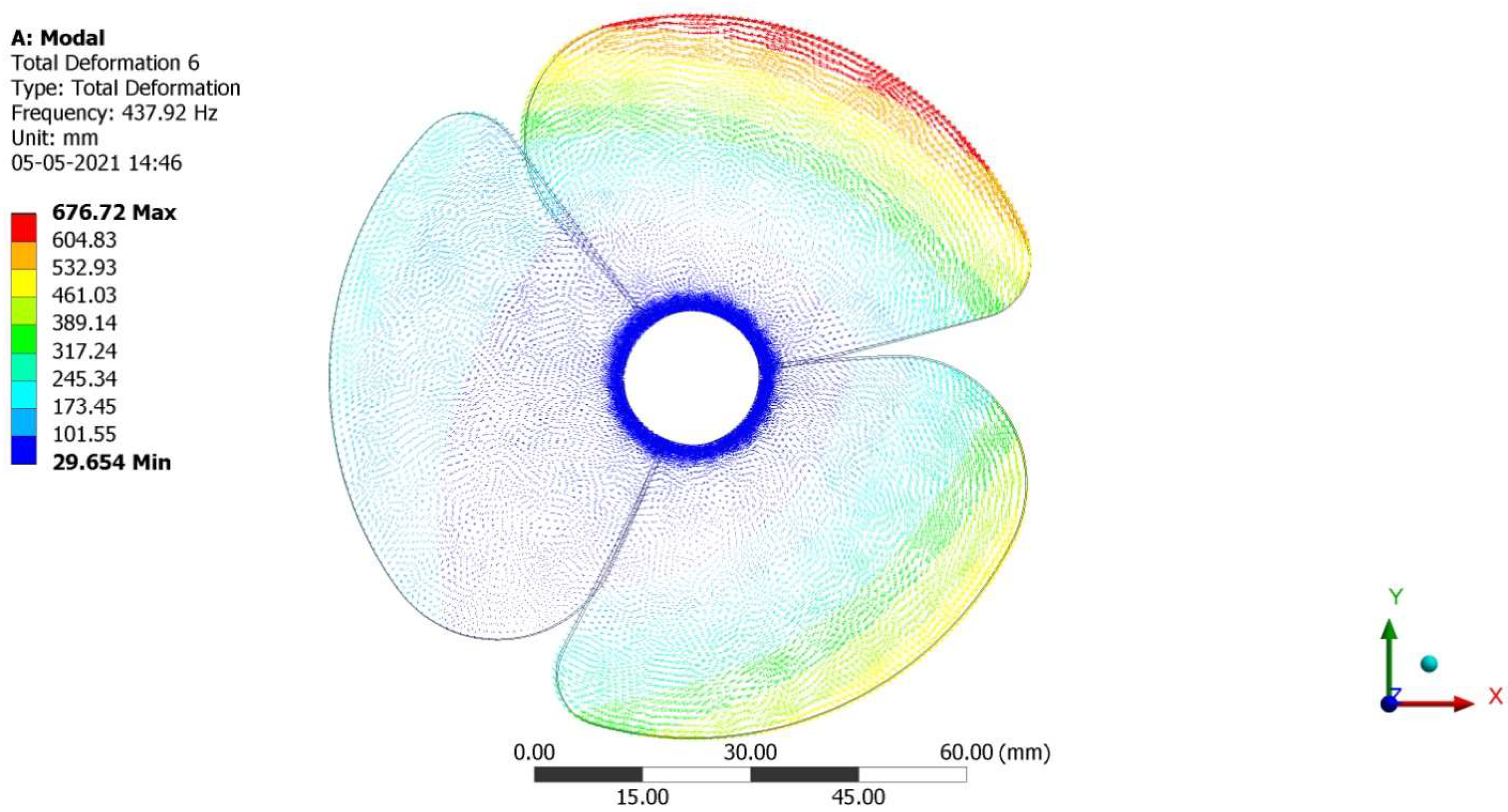
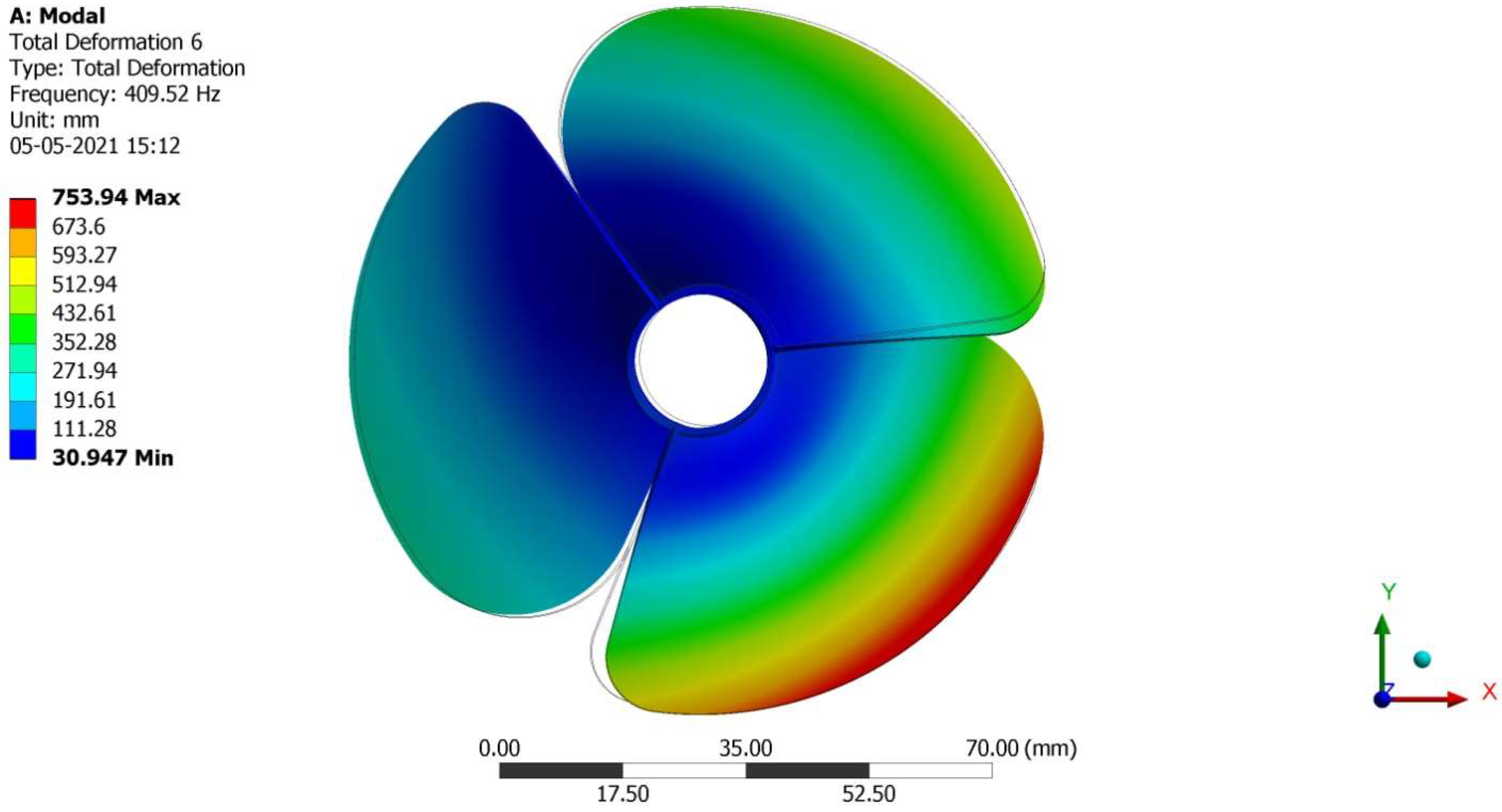
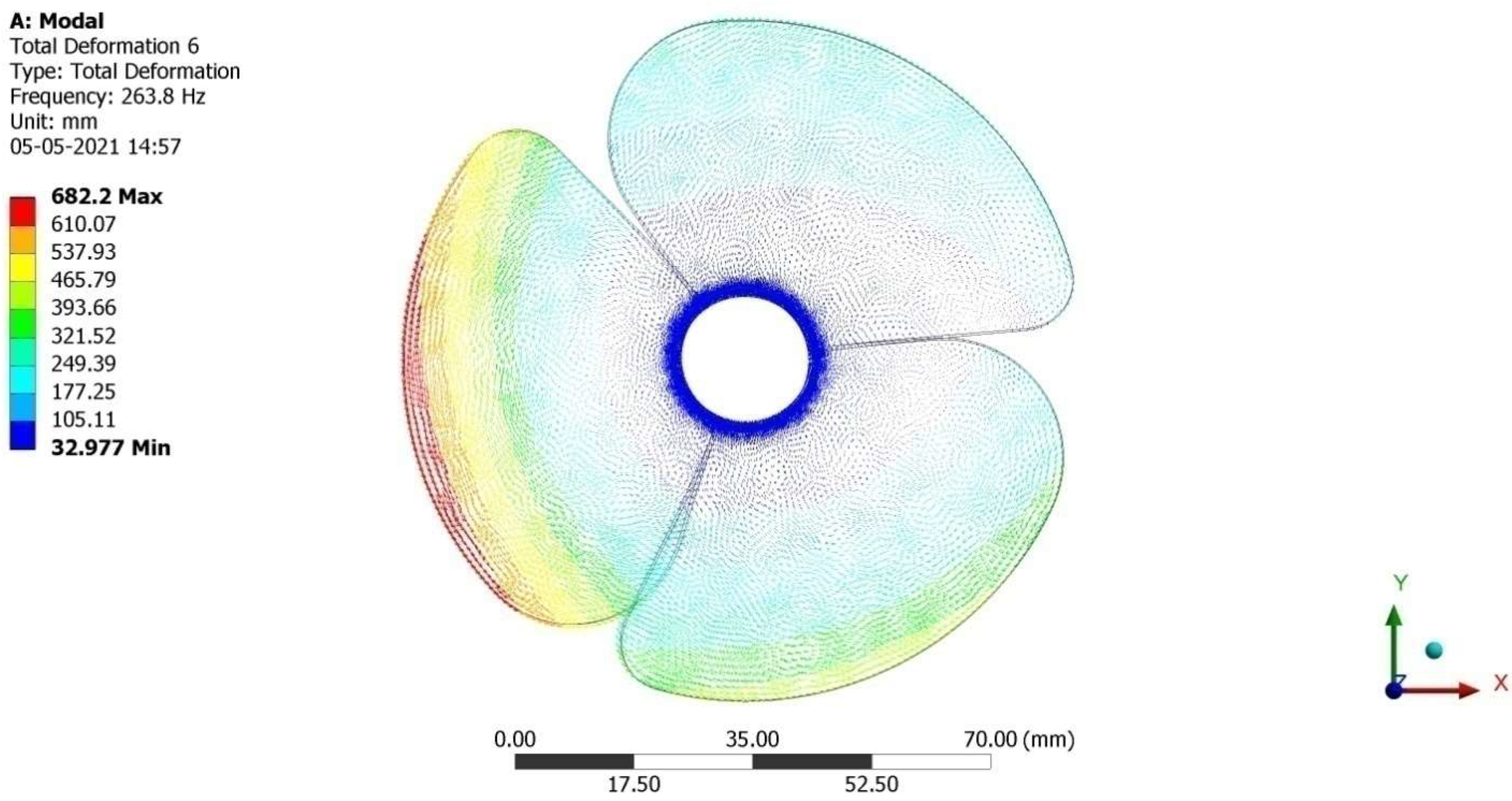
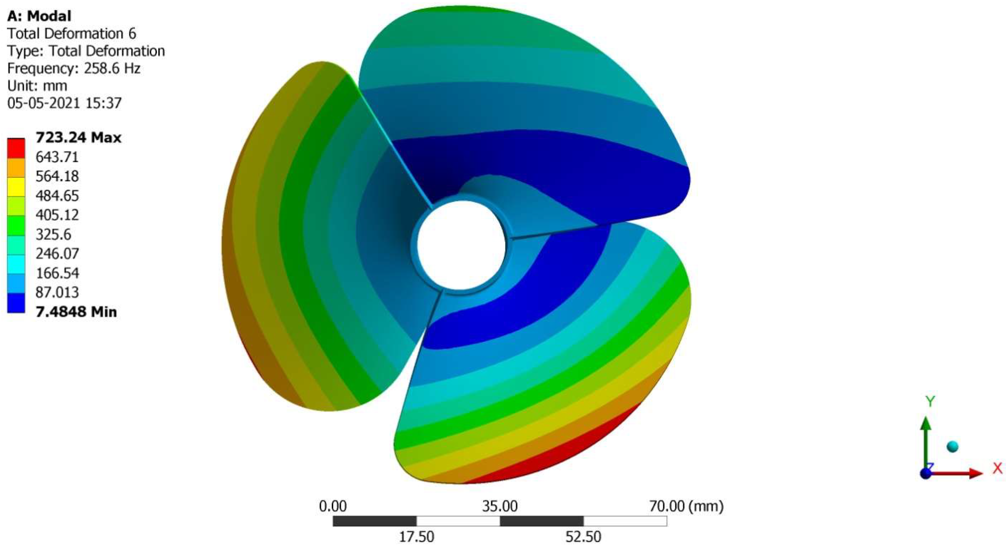
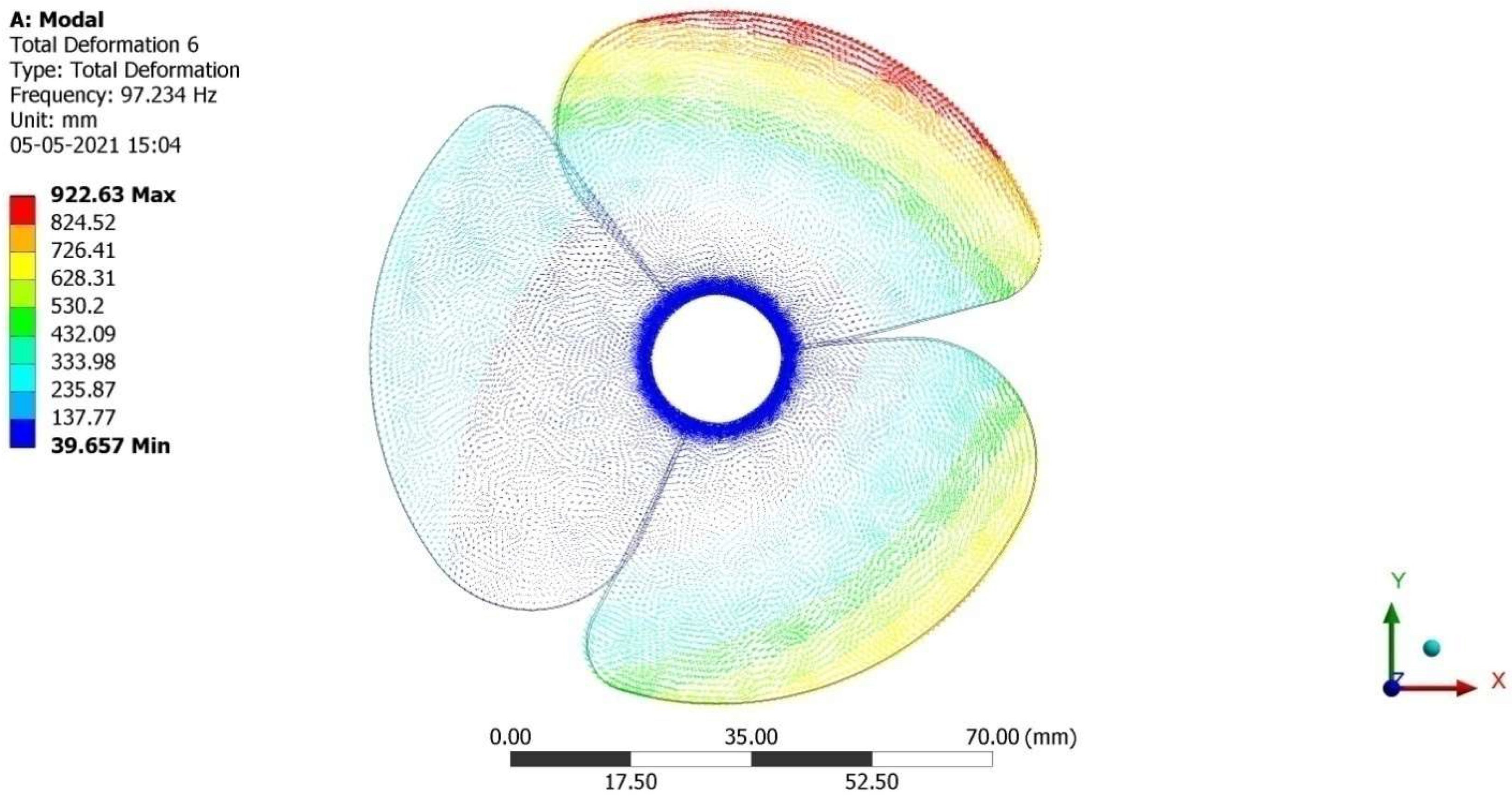
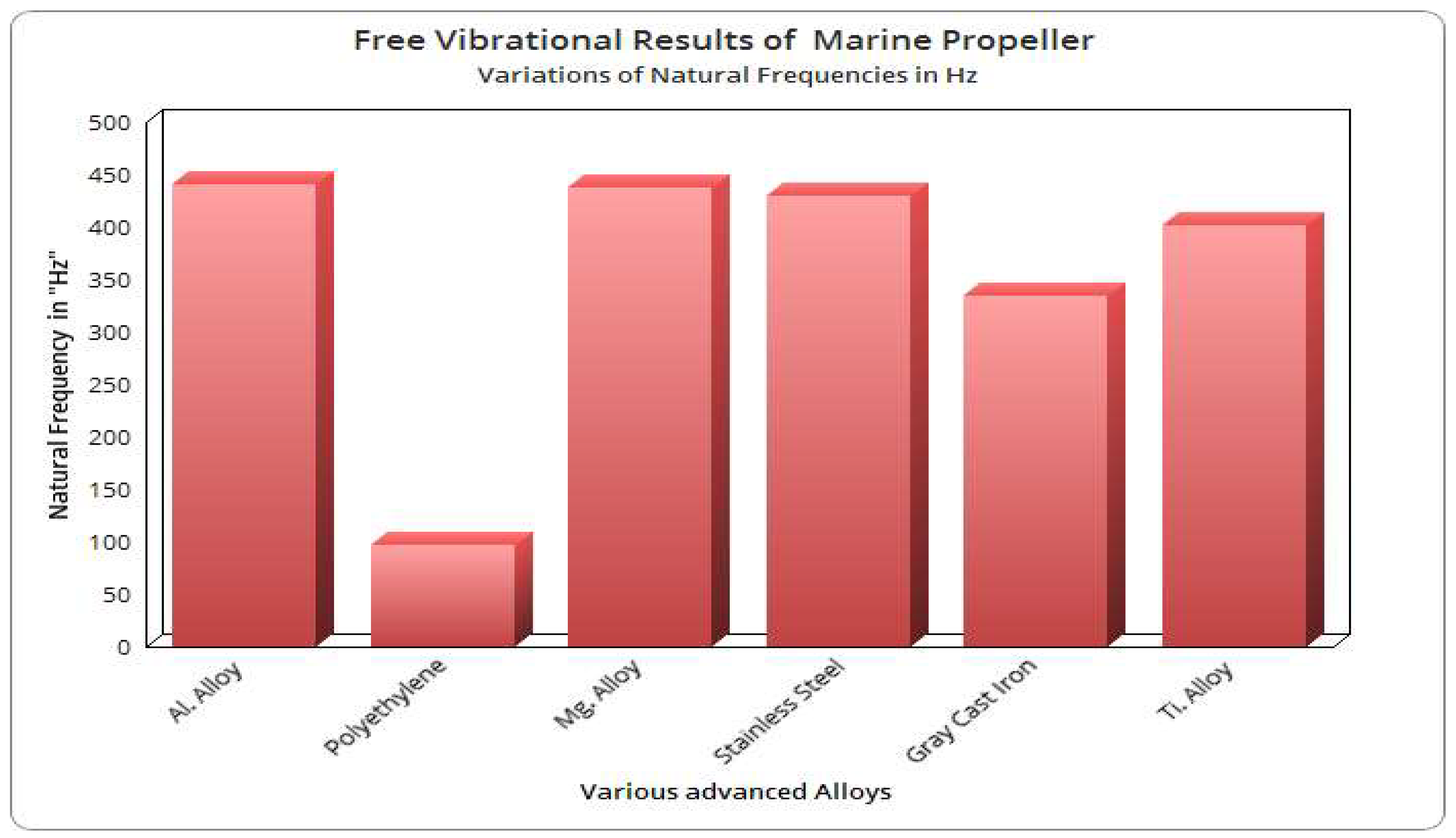
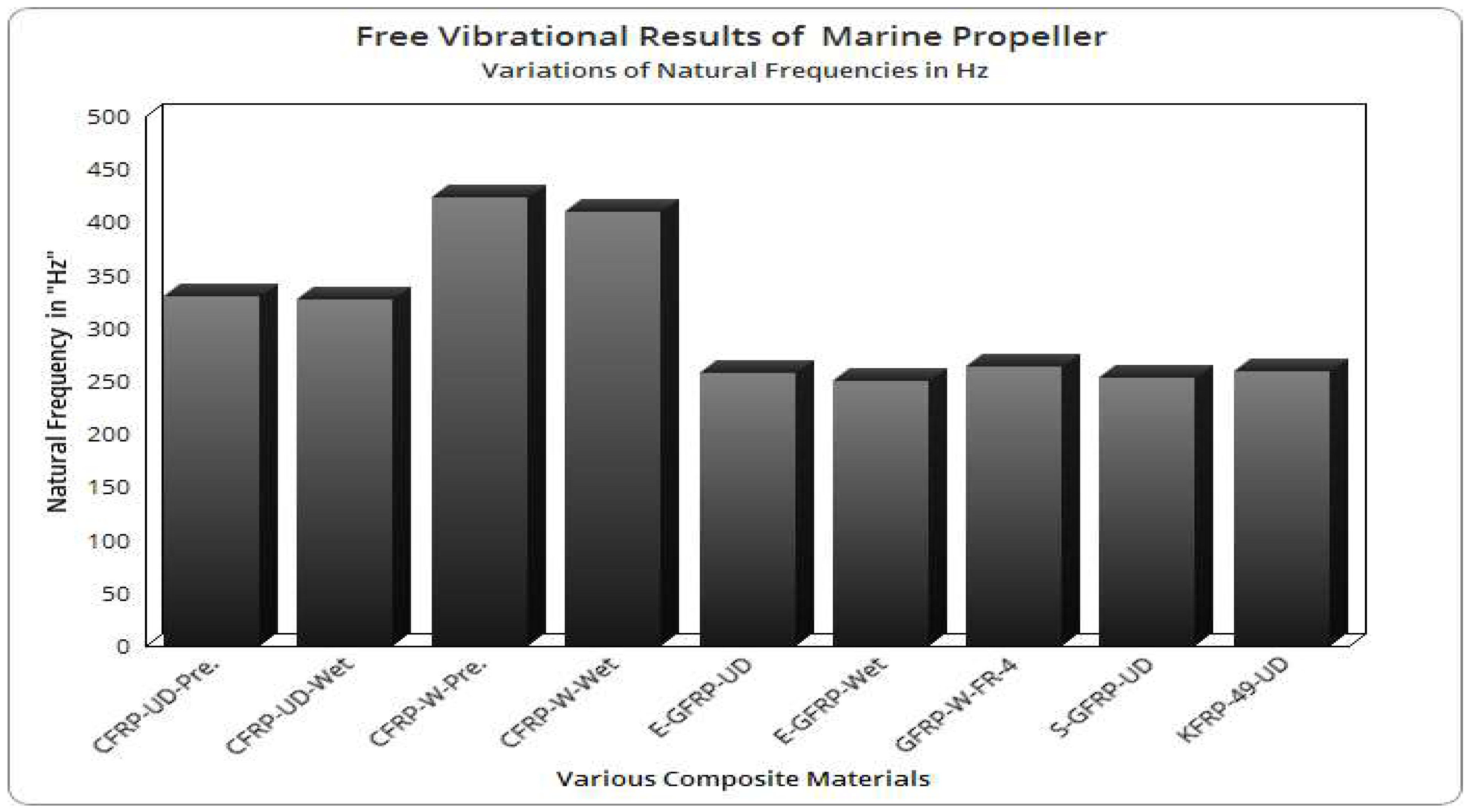
4.2. Free Vibrational Results

The US propeller’s natural frequency is determined and put to beneficial use. The propeller will fail if it runs at its abnormal frequency, but when it runs at a lower frequency, we may maximize displacement and thus generate power. In addition, the propeller should not be allowed to stretch beyond its elastic limit, as doing so would result in undesirable permanent deformation. Under these circumstances, the US’s propeller can be displaced to generate energy without cracking. This rotor is subjected to free vibrational studies with the aforementioned boundary conditions for 15different, relatively light materials. Figure 44, Figure 45, Figure 46, Figure 47 and Figure 48 show the computational results based natural frequencies of the US propeller. Following a free vibrational analysis, the optimal mode shape is selected as the sixth mode shape for both deformation and natural frequency. In Figure 44, we see the results for aluminium alloy; in Figure 45, for CFRP UD Prepreg-based composites; in Figure 46, for E-Glass Wet-based composites; in Figure 47, for KFRP-UD-49-based composites; and in Figure 48, for Polyethylene-related composites.

4.3. Comparative Analysis

The complete results of calculating the natural frequencies of several different lightweight materials are shown in Figure 49 and Figure 50.
Natural frequency results for lightweight alloys are shown in Figure 49, while those for lightweight composites are shown in Figure 50.

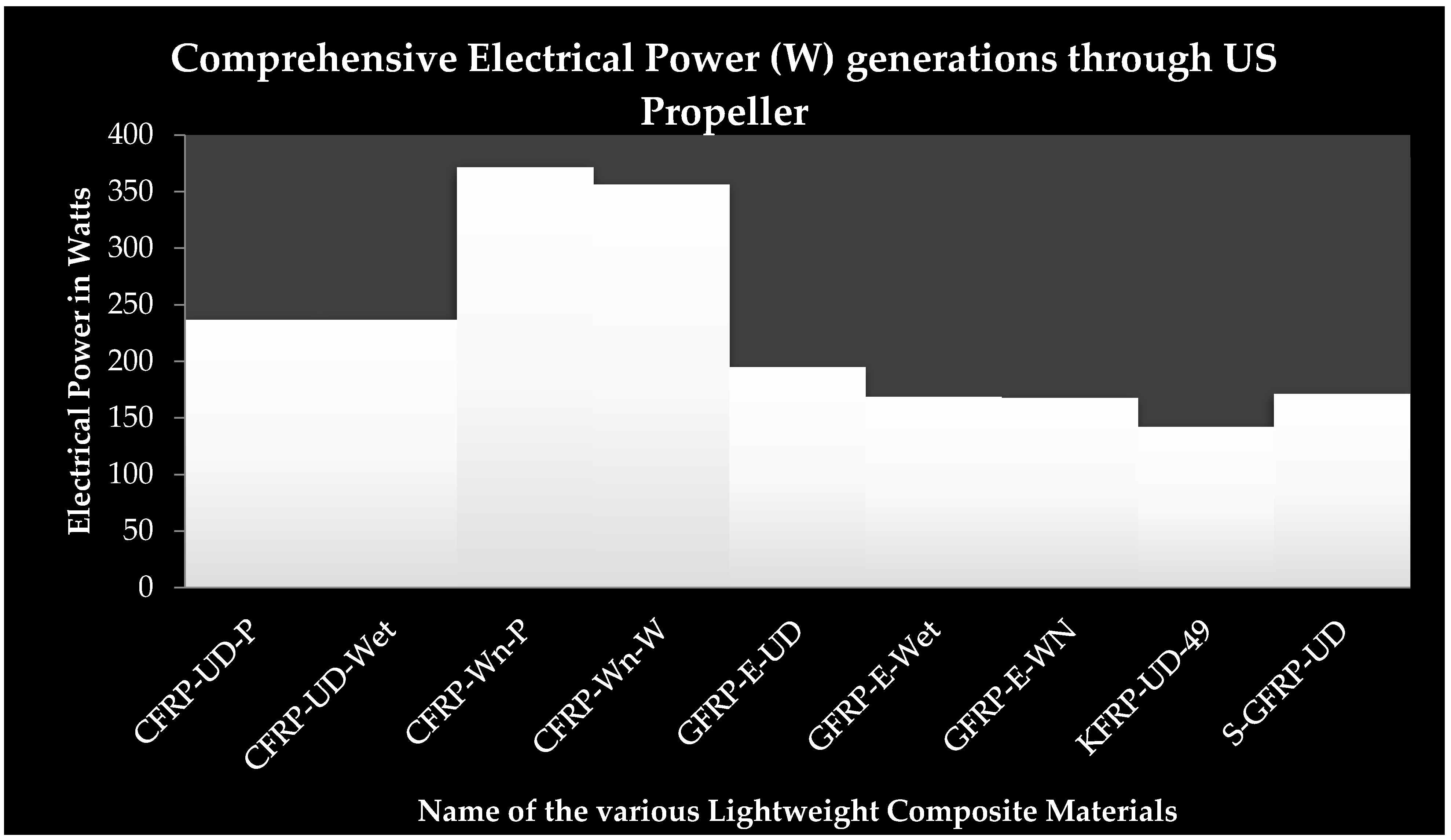
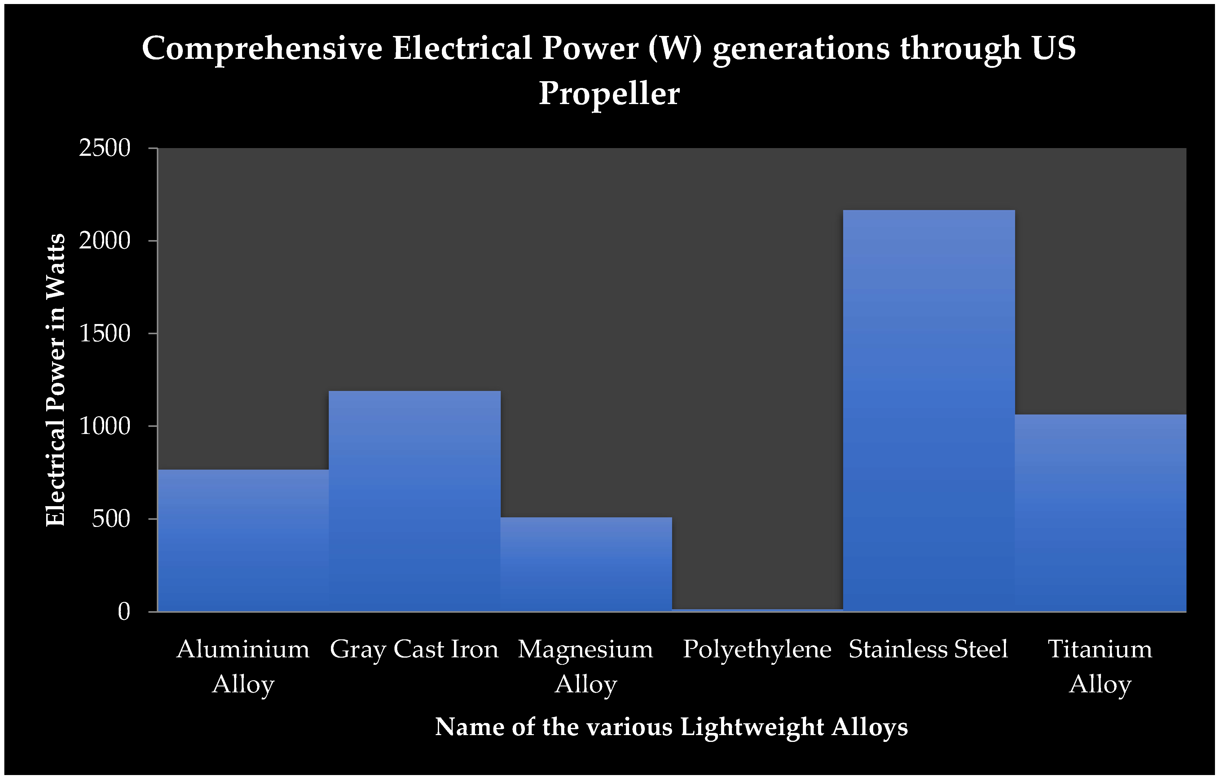
4.4. PVEH Based Electricity Estimation

Figure 51 depicts the planned alternate energy extraction using a US propeller.
Analytical Equations (33) and (34) are supplied, which were derived from calculations and described in the literature study [54] to provide the compositional components of electricity generation through the PVEH patch. All these analytical equations rely on three data points gleaned from either computational modelling or a review of the relevant literature. The three main inputs are natural frequencies, uniformly distributed loads based on hydrodynamic pressure, and dielectric constants. In the scenario where CHA and CVA approximate hydrodynamic pressure and free vibrational frequencies, the dielectric constants are acquired via a literature review [35,36,37,38,39,40,41,42,43,44,45,46,47,48,49,50,51,52,53,54,55,56,57].
P Intermediate US ,   P = ( C LWM US , P ) 2 × ( P UDL US , P ) 2 × ( f US , P ) 2                         × 18 × T PP [ ( W US , P ) × ( L PP US , P ) 2 × ( [ t US , P ] + [ T PP US , P ] ) 4 ]                         × ρ lmw [ 1 + f US , P × ε × ( ρ LWM ) ]
P Final US ,   P = ( P Intermediate US ,   P )                             × ( ( 0.0278 5 ) ( 0.167 L 4 ) + ( 0.4167 L 2 3 ) ( 0.5 L 3 2 )                             + ( 0.25 L 4 ) )
where, “ C LWM US , P ” is piezoelectric material constant, “ P UDL US , P ” is fluid dynamic load in Newton, “ f US , P ” is free vibrational natural frequency in Hertz, “ W US , P ” is US’s propeller width in meter, “ L PP US , P ” is piezoelectric patch length in meter, “ t US , P ” is US’s propeller thickness in meter, “ T PP US , P ” is piezoelectric patch thickness in meter, “ ρ LWM ” is density of the lightweight material, “ε” is permittivity of the same lightweight materials. For this work, the sample calculation is taken and so the imposed material is CFRP-Woven-Wet. The input values are: C LWM US , P = 0.12; Surface area of hydro propeller (single side of single blade) = 0.0024806 m²; fluid dynamic pressure acting on US’s propeller = 29,962.5 N/m2; fluid dynamic Force ( P UDL US , P ) (single side of single blade) = 29,962.5 × 0.002481 = 74.325 N; f US , P = 409.52 Hz; W US , P =0.040708 m; L PP US , P = 0.072097 m; t US , P = 0.00099997 m; T PP US , P = 0.00099997 m; ρ LWM = 1451 kg/m3; ε = Dielectric   Constant = 5 × 10 12 ; P Final US ,   P = 356.45   Watts . This calculation is repeated for the remaining 14lightweight materials, and the electricity results are shown in Figure 52 and Figure 53.
Compared to other lightweight materials, the vibrational characteristics of aluminium alloy (shown in Figure 52 and Figure 53) make it clear that it performed admirably. Furthermore, this increased vibration resulted in a greater electrical current being generated by the aluminium alloy, making it a prime candidate for use in real-life scenarios.

5. Conclusions

The conceptual designs of entire US models are completed with the help of CATIA. The standard theoretical formula and computational approaches are used for estimating aerodynamic and hydrodynamic evaluation parameters such as thrust, drag, lift, and weight. The advanced CFD tool, i.e., ANSYS Fluent, is used for the entire comparative CFD analyses. Two major works are executed from these approaches: components selection and deployment tests. All manoeuvres in either setting can be carried out with the help of the thrust table, which also helps determine the optimal propeller RPM. Even though model 2 has a similar drag value as model 1, its capability to move faster underwater and the streamlined shape of the body and the manoeuvrability makes it optimized for underwater operations, provided the components required for the application are limited within the fuselage of the design. Thus, the proposed US with a unique Becker-adopted vertical stabilizer is the perfect one to complete the mission successfully. It is intended to install PVEH-based energy-extracting patches on the hydro-propeller surfaces to make up for the US’s excessive energy consumption in the water sector. The unique analytical calculations are incorporated into this energy extraction concept. Fluid-structure interaction-based advanced computational simulation is carried out on the propeller up to the 300-m depth, and the suitable lightweight material is shortlisted. After extensive testing in a deployment environment, the modelled US is found to be ready for immediate deployment thanks to state-of-the-art computational resources.

Author Contributions

Conceptualization, V.R. and R.M.; methodology, V.R., D.K.J. and R.M.; software, V.R. and R.M.; validation, V.R., R.M. and H.A.Z.A.-b.; formal analysis, V.R. and H.A.Z.A.-b.; investigation, V.R., S.P. and P.R.; resources, V.R., D.K.J. and R.M.; data curation, V.R. and D.K.J.; writing—original draft preparation, S.P.; writing—review and editing, S.P., P.R. and V.R.; visualization, H.A.Z.A.-b. and P.R.; supervision, M.A.-B.; project administration, P.R.; funding acquisition, P.R. All authors have read and agreed to the published version of the manuscript.

Funding

This work was supported by a Universiti Sains Malaysia, Bridging GRA with Project No: 304/PAERO/6316608.

Data Availability Statement

Not applicable.

Acknowledgments

The Aircraft Design and Analyses Laboratory, Department of Aeronautical Engineering, Kumaraguru College of Technology (KCT), Coimbatore-641049, Tamil Nadu, India, supports the computational resources used in this work. As a result, the authors of this article would like to thank all of the top management and professionals.

Conflicts of Interest

The authors declare no conflict of interest.

Abbreviations

SymbolDescription
W Payload Weight of the payloads (kg)
W Overall Total weight of the US (kg)
W S Wing loading of this US’s rectangular wing (kg/m2)
S Wing Planform area of the US’s rectangular wing (m2)
b wing Wingspan of the rectangular wing (m)
C Wing root Root chord of the rectangular wing (m)
L Fuselage Length of the US fuselage (m)
AR Wing Aspect ratio of the rectangular wing
ƞ Design efficiency
D Fuselage Diameter of US Fuselage (m)
λ Taper ratio of lifting platform
S V Tail Planform area of the vertical stabilizer (m2)
b V Tail Tail-span of the vertical stabilizer (m)
C V Tail root Root chord of the vertical stabilizer (m)
D Fuselage Maximum Maximum diameter of the US fuselage (m)
L Fuselage Uniform   Cross   Section Length of the uniform cross section of the US fuselage (m)
L Fuselage Varying   Cross   Section Length of the varying cross section of the US fuselage (m)
D Fuselage Varying   Cross   Section Diameter of the varying cross section of the US fuselage (m)
mSlope of the linearized curvy position of fuselage
bConstant of the linearized curvy position of fuselage
T Required Required thrust of the US propeller (N)
λ Optimum US , P Optimum tip speed ratio of US propeller
B T Thrust coefficient of US propeller
V FS Forward velocity of the US (m/s)
D US ,   P Diameter of the US fuselage (m)
K 0 US ,   P ,   K 1 US ,   P ,
K 2 US ,   P , K 3 US , P ,
K 4 US , P ,   K 5 US , P
Design constants involved in the estimation of various radius and pitch of the US propeller
R US , P Radius of the US fuselage (m)
V fluid Fluid dynamic velocity (m/s)
u x fluid ,   v y fluid ,   w z fluid Fluid dynamic velocities in different directions (m/s)
ρ fluid Density of the working fluid (kg/m3)
p Change in fluid dynamic pressure with respect to direction
μ Bulk viscosity (Pa-s)
k Thermal conductivity (W/mK)
T Temperature (K)
R Specific gas constant (J/(kgK))
F ¯ Averaged force acting on the control volume in CFD (N)
u ¯ Averaged velocity acting on the control volume in CFD (m/s)
C LWM US , P piezoelectric material constant
P UDL US , P fluid dynamic load (N)
f US , P free vibrational natural frequency (Hz)
W US , P US’s propeller width (m)
L PP US , P piezoelectric patch length (m)
t US , P US’s propeller thickness (m)
T PP US , P piezoelectric patch thickness (m)
ρ LWM density of the lightweight material (kg/m3)
εpermittivity of the same lightweight materials

References

  1. Wang, Q.; Wu, S.; Hong, W.; Zhuang, W.; Wei, Y. Submersible Unmanned Aerial Vehicle: Configuration Design and Analysis Based on Computational Fluid Dynamics. MATEC Web Conf. 2017, 95, 07023. [Google Scholar] [CrossRef] [Green Version]
  2. Li, Y.; Hu, J.; Zhao, Q.; Pan, Z.; Ma, Z. Hydrodynamic Performance of Autonomous Underwater Gliders with Active Twin Undulatory Wings of Different Aspect Ratios. J. Mar. Sci. Eng. 2020, 8, 476. [Google Scholar] [CrossRef]
  3. Tangorra, J.L.; Davidson, S.N.; Hunter, I.W.; Madden, P.G.A.; Lauder, G.V.; Dong, H.; Bozkurttas, M.; Mittal, R. The Development of a Biologically Inspired Propulsor for Unmanned Underwater Vehicles. IEEE J. Ocean. Eng. 2007, 32, 533–550. [Google Scholar] [CrossRef] [Green Version]
  4. Joung, T.-H.; Sammut, K.; He, F.; Lee, S.-K. Shape optimization of an autonomous underwater vehicle with a ducted propeller using computational fluid dynamics analysis. Int. J. Nav. Arch. OceanEng. 2012, 4, 44–56. [Google Scholar] [CrossRef] [Green Version]
  5. Xuel, G.; Liu, Y.; Chen, Z.; Li, S. Motion Model of Fish-like Underwater Vehicle and its Effect on Hydrodynamic Performance. In Proceedings of the 2018 11th International Symposium on Mechatronics and its Applications (ISMA), Sharjah, United Arab Emirates, 4–6 March 2018. [Google Scholar] [CrossRef]
  6. Gao, A.; Techet, A.H. Design considerations for a robotic flying fish. In Proceedings of the OCEANS’11MTS/IEEEKONA, Waikoloa, HI, USA, 19–22 September 2011. [Google Scholar] [CrossRef]
  7. Wang, Z.; Li, Y.; Wang, A.; Wang, X. Flying Wing Underwater Glider: Design, Analysis, and Performance Prediction. In Proceedings of the 2015 International Conference on Control, Automation and Robotics, Singapore, 20–22 May 2015. [Google Scholar] [CrossRef]
  8. Mathaiyan, V.; Murugesan, R.; Madasamy, S.K.; Gnanasekaran, R.K.; Sivalingam, S.; Jung, D.W. Conceptual Design and Numerical analysis of an Unmanned Amphibious Vehicle. AIAA Scitech 2021 Forum 2021, 1285. [Google Scholar] [CrossRef]
  9. Javaid, M.Y.; Ovinis, M.; Hashim, F.B.; Maimun, A.; Ahmed, Y.M.; Ullah, B. Effect of wing form on the hydrodynamic characteristics and dynamic stability of an underwater glider. Int. J. Nav. Arch. Ocean Eng. 2017, 9, 382–389. [Google Scholar] [CrossRef] [Green Version]
  10. Alam, K.; Ray, T.; Anavatti, S.G. Design and construction of an autonomous underwater vehicle. Neurocomputing 2014, 142, 16–29. [Google Scholar] [CrossRef]
  11. Kumar, V.P.; Kumar, S.K.; Pandian, K.S.; Ashraf, E.; Selvan, K.T.T.; Vijayanandh, R. Conceptual Design and Hydrodynamic Research On Unmanned Aquatic Vehicle. Int. J. Innov. Technol. Explor. Eng. 2019, 8, 121–127. [Google Scholar] [CrossRef]
  12. Vasudev, K.L. Review of Autonomous Underwater Vehicles, Autonomous VehiclesBook; Intech Open Limited: London, UK, 2018; ISBN 978-1-83968-191-2. [Google Scholar] [CrossRef]
  13. Amin, O.M.; Karim, A.; Saad, A.H. Development of a highly maneuverable unmanned underwater vehicle on the basis ofquad-copter dynamics. AIP Conf. Proceed. 2017, 1919, 020009. [Google Scholar]
  14. Pandian, R.S.; Vijayanandh, R.; Kumar, S.K.; Kumar, V.P.; Ramesh, M.; Kumar, M.S.; Kumar, G.R. Comparative Hydrodynamic Investigations on Unmanned Aquatic Vehicle for Ocean Applications. In Recent Trends in Mechanical Engineering; Lecture Notes in Mechanical Engineering Book Series(LNME); Springer: Berlin/Heidelberg, Germany, 2021; ISBN 978-981-16-2086-7. [Google Scholar] [CrossRef]
  15. Nesteruk, I.; Passoni, G.; Redaelli, A. Shape of Aquatic Animals and Their Swimming Efficiency. J. Mar. Biol. 2014, 2014, 1–9. [Google Scholar] [CrossRef] [Green Version]
  16. Bettle, M.C.; Gerber, A.G.; Watt, G.D. Using reduced hydrodynamic models to accelerate the predictor–corrector convergenceofimplicit6-DOFURANS submarine manoeuvring simulations. Comput. Fluids 2014, 102, 215–236. [Google Scholar] [CrossRef] [Green Version]
  17. Wang, Y.; Zhang, Y.; Zhang, M.; Yang, Z.; Wu, Z. Design and flight performance of hybrid underwater glider with controllable wings. Int. J. Adv. Robot. Syst. 2017, 14, 1–12. [Google Scholar] [CrossRef] [Green Version]
  18. Qiu, S.; Cui, W. An Overview on Aquatic Unmanned Aerial Vehicles. Ann. Rev. Res. 2019, 5, 555663. [Google Scholar] [CrossRef]
  19. Wang, Z.-J.; Nie, Z.-Q.; Li, J.-X.; Ma, Y. Conceptual Design of a Water-air Amphibious Unmanned Vehicle. DES techTrans. Comput. Sci. Eng. 2019, 2018, 000781–000786. [Google Scholar] [CrossRef]
  20. Uiblein, F.; Cruz, N.A. Deep-Sea Fish Behavioral Responses to Underwater Vehicles: Differences among Vehicles, Habitats and Species; Autonomous Underwater Vehicles; Cruz, N., Ed.; IntechOpen: London, UK, 2011; ISBN 978-953-307-432-0. [Google Scholar]
  21. Bozkurttas, M.; Tangorra, J.; Lauder, G.; Mittal, R. Understanding the Hydrodynamics of Swimming from Fish Fins to Flexible Propulsors for Autonomous Underwater Vehicles. Adv. Sci. Technol. 2008, 58, 193–202. [Google Scholar] [CrossRef]
  22. Fish, F.E. Wing design and scaling of flying fish with regard to flight performance. J. Zoöl. 1990, 221, 391–403. [Google Scholar] [CrossRef]
  23. Wang, J.; Wainwright, D.K.; Lindengren, R.E.; Lauder, G.V.; Dong, H. Tuna locomotion: A computational hydrodynamic analysis of finlet function. J. R. Soc. Interface 2020, 17, 20190590. [Google Scholar] [CrossRef] [Green Version]
  24. Ignacio, L.C.; Victor, R.R.; Del Rio, R.; Pascoal, A. Optimized design of an autonomous underwater vehicle, for exploration in the Caribbean Sea. Ocean Eng. 2019, 187, 106184. [Google Scholar] [CrossRef]
  25. Park, H.; Choi, H. Aerodynamic characteristics of flying fish in gliding flight. J. Exp. Biol. 2010, 213 Pt 19, 3269–3279. [Google Scholar] [CrossRef] [PubMed] [Green Version]
  26. Allotta, B.; Costanzi, R.; Monni, N.; Pugi, L.; Ridolfi, A.; Vettori, G. Design and Simulation of an Autonomous Underwater Vehicle. In Proceedings of the European Congress on Computational Methods in Applied Sciences and Engineering ECCOMAS, Vienna, Austria, 10–14 September 2012. [Google Scholar]
  27. Gao, T.; Wang, Y.; Pang, Y.; Cao, J. Hull shape optimization for autonomous underwater vehicles using CFD. Eng. Appl. Comput. Fluid Mech. 2016, 10, 599–607. [Google Scholar] [CrossRef] [Green Version]
  28. Vijayanandh, R.; Senthil Kumar, M.; Rahul, S.; Thamizhanbu, E.; Durai Isaac Jafferson, M. Conceptual Design and Comparative CFD Analyse son Unmanned Amphibious Vehicle for Crack Detection. Proceedings of UASG 2019, Roorkee, India, 6–7 April 2019; Lecture Notes in CivilEngineering. Springer: Cham, Switzerland, 2019. ISBN 978-3-030-37393-1. [Google Scholar] [CrossRef]
  29. Raja, V.; Solaiappan, S.K.; Kumar, L.; Marimuthu, A.; Gnanasekaran, R.K.; Choi, Y. Design and Computational Analyses of Nature Inspired Unmanned Amphibious Vehicle for Deep Sea Mining. Minerals 2022, 12, 342. [Google Scholar] [CrossRef]
  30. Vijayanandh, R.; Venkatesan, K.; Kumar, R.R.; Kumar, M.S.; Jagadeeshwaran, P. Theoretical and Numerical Analyses on Propulsive Efficiency of Unmanned Aquatic Vehicle’s Propeller. J. Phys. Conf. Ser. 2020, 1504, 012004. [Google Scholar] [CrossRef]
  31. Vijayanandh, R.; Venkatesan, K.; Kumar, M.S.; Kumar, G.R.; Jagadeeshwaran, P. Comparative fatigue life estimations of Marine Propeller by using FSI. J. Phys. Conf. Ser. 2020, 1473, 012018. [Google Scholar] [CrossRef]
  32. Jiang, Y.; Raji, A.P.; Raja, V.; Wang, F.; Al-Bonsrulah, H.A.Z.; Murugesan, R.; Ranganathan, S. Multi–Disciplinary Optimizations of Small-Scale Gravitational Vortex Hydropower (SGVHP) System through Computational Hydrodynamic and Hydro–Structural Analyses. Sustainability 2022, 14, 727. [Google Scholar] [CrossRef]
  33. Raja, V.; Raji, A.P.; Madasamy, S.K.; Mathaiyan, V.; Kandasamy, S.; Subramaniam, I.P.; Kandasamy, K.; Murugesan, R.; Rajapandi, R.; Jayaram, D.K.; et al. Comparative Estimations of Hydrodynamic Analysis on Unmanned Aquatic Vehicle’s Propeller by using an advanced [CFD with MRF] Approach. In Proceedings of the AIAA Propulsion and Energy 2021 Forum, Virtual Event, 9–11 August 2021. [Google Scholar] [CrossRef]
  34. Raja, V.; AL-bonsrulah, H.A.Z.; Raji, A.P.; Madasamy, S.K.; Ramaiah, M.; Gnanasekaran, R.K.; Kulandaiyapan, N.K.; Al-Bahrani, M. Design and multi-disciplinary computational investigations on PVEH patches attached horizontal axis hybrid wind turbine system for additional energy extraction in HALE UAVs. IET Renew. Power Gener. 2022, 16, 1–27. [Google Scholar] [CrossRef]
  35. Du, S.; Jia, Y.; Seshia, A. Maximizing Output Power in a Cantilevered Piezoelectric Vibration Energy Harvester by Electrode Design. J. Phys. Conf. Ser. 2015, 660, 012114. [Google Scholar] [CrossRef]
  36. Kulandaiyaappan, N.K.; Gnanasekaran, R.K.; Raja, V.; Bernard, F.A.; Murugesan, R.; Madasamy, S.K.; Mathaiyan, V.; Raji, A.P.; K Asher, P.; Ponmariappan, J. Optimization of High Payload Unmanned Aerial Vehicle’s Propellers based on Energy Formation by using Computational Vibrational Analyses. In Proceedings of the AIAA Propulsion and Energy 2021 Forum, Virtual Event, 9–11 August 2021. [Google Scholar] [CrossRef]
  37. Osuchukwu, N.; Shpanin, L. Feasibility Study of the Quadcopter Propeller Vibrations for the Energy Product. Int. J. Mech. Mechatron. Eng. 2017, 11, 313–319. [Google Scholar] [CrossRef]
  38. Anton, S.R.; Inman, D.J. Performance modeling of unmanned aerial vehicles with on-board energy harvesting. Act. Passiv. Smart Struct. Integr. Syst. 2011, 7977, 12–27. [Google Scholar] [CrossRef]
  39. Anton, S.R.; Erturk, A.; Inman, D.J. Investigation of a Multifunctional energy harvesting and energy-storage wing spar for unmanned aerial vehicles. J. Aircr. 2012, 49, 292–301. [Google Scholar] [CrossRef] [Green Version]
  40. Mohammadi, S.; Cheraghi, K.; Khodayari, A. Piezoelectric vibration energy harvesting using strain energy method. Eng. Res. Express 2019, 1, 015033. [Google Scholar] [CrossRef]
  41. Kress, R.; Lorenz, E.L. Marine Propeller Selection; Section 1: Works 700010–700182; SAE Transactions: Warrendale, PA, USA, 1970; Volume 79, pp. 334–345. [Google Scholar]
  42. Sahoo, S.S.; Singh, V.K.; Panda, S.K. Experimental and simulation study of flexural behaviour of woven Glass/Epoxy laminated composite plate. IOP Conf. Ser. Mater. Sci. Eng. 2015, 75, 012017. [Google Scholar] [CrossRef]
  43. Rajagurunathan, M.; Raj Kumar, G.; Vijayanandh, R.; Vishnu, V.; Rakesh Kumar, C.; Mohamed Bak, K. The Design Optimization of the Circular Piezoelectric Bimorph Actuators Using FEA. Int. J. Mech. Prod. Eng. Res. Dev. 2018, 8, 410–422. [Google Scholar]
  44. Kumar, M.S.; Krishnan, A.; Vijayanandh, R. Vibrational Fatigue Analysis of NACA63215 Small Horizontal Axis Wind Turbine blade. Mater. Today Proc. 2018, 5, 6665–6674. [Google Scholar] [CrossRef]
  45. Elahi, H.; Eugeni, M.; Gaudenzi, P.A. Review on Mechanisms for Piezoelectric-Based Energy Harvesters. Energies 2018, 11, 1850. [Google Scholar] [CrossRef]
  46. DeMarqui, C., Jr.; Vieira, W.G.R.; Erturk, A.; Inman, D.J. Modeling and Analysis of Piezoelectric Energy Harvesting From Aeroelastic Vibrations Using the Doublet-Lattice Method. J. Vib. Acoust. 2011, 133, 11003. [Google Scholar] [CrossRef] [Green Version]
  47. Dobbs, S.; Yu, Z.; Anderson, K.R.; Franco, J.A.; Deravanessian, A.E.; Lin, A.; Ahn, A. Design of an In-flight Power Generation And Storage System for UAVs. In Proceedings of the 2018 IEEE Conference on Technologies for Sustainability, Long Beach, CA, USA, 11–13 November 2018; pp. 1–8. [Google Scholar] [CrossRef]
  48. Williams, C.D.; Curtis, T.L.; Doucet, J.M.; Issac, M.T.; Azarsina, F. Effects of Hull Length on the Hydrodynamic Loads on a Slender Underwater Vehicle during Manoeuvres. In Proceedings of the OCEANS2006, Boston, MA, USA, 18–21 September 2006; pp. 1–6. [Google Scholar] [CrossRef] [Green Version]
  49. Sakaki, A.; Kerdabadi, M.S. Experimental and numerical determination of the hydrodynamic coefficients of an autonomous underwater vehicle. Sci. J. Marit. Univ. Szczec. 2020, 62, 124–135. [Google Scholar]
  50. Barlow, J.B.; Guterres, R.; Ranzenbach, R. Experimentalparametricstudyofrectangularbodieswithradiusededgesingroundeffect. J. Wind Eng. Ind. Aerodyn. 2001, 89, 1291–1309. [Google Scholar] [CrossRef]
  51. Cory, R.; Tedrake, R. Experiments in fixed-wing UAV perching. In Proceedings of the AIAA Guidance, Navigation and Control Conference and Exhibit, Honolulu, HI, USA, 18–21 August 2008; pp. 1–12. [Google Scholar]
  52. Xu, G.; Zhang, Y.; Ji, S.; Cheng, Y.; Tian, Y. Research on computer vision-based for UAV autonomous landing on a ship. Pattern Recognit. Lett. 2009, 30, 600–605. [Google Scholar] [CrossRef]
  53. Pisanich, G.; Morris, S. Fielding an amphibious UAV: Development, results, and lessons learned. In Proceedings of the 21st Digital Avionics Systems Conference, Irvine, CA, USA, 27–31 October 2002; Volume 2, p. 8C4-1-8C4-9. [Google Scholar]
  54. Siddall, R.; Kovač, M. Launching the Aqua MAV: Bioinspired design for aerial–aquatic robotic platforms. Bioinspir. Biomim. 2014, 9, 031001. [Google Scholar] [CrossRef]
  55. Schwarzbach, M.; Laiacker, M.; Mulero-Pázmány, M.; Kondak, K. Remote water sampling using flying robots. In Proceedings of the 2014 International Conference on Unmanned Aircraft Systems (ICUAS), Orlando, FL, USA, 27–30 May 2014; pp. 72–76. [Google Scholar]
  56. Ore, J.P.; Elbaum, S.; Burgin, A.; Detweiler, C. Autonomous aerial water sampling. J. Field Robot. 2015, 32, 1095–1113. [Google Scholar] [CrossRef]
  57. Yang, X.; Wang, T.; Liang, J.; Yao, G.; Zhao, W. Submersible unmanned aerial vehicle concept design study. In Proceedings of the 2013 Aviation Technology, Integration, and Operations Conference, Los Angeles, CA, USA, 12–14 August 2013; p. 442. [Google Scholar]
Figure 1. US’s Mission Profile of this proposed work.
Aerospace 09 00652 g001
Figure 2. A typical comprehensive report of historical relationships between payload weight and overall weight of the USs.
Aerospace 09 00652 g002
Figure 3. A typical top view of the imposed rectangular wing.
Aerospace 09 00652 g003
Figure 4. A typical front view of the developed half portioned fuselage.
Aerospace 09 00652 g004
Figure 5. A typical side view of the modelled fuselage of US.
Aerospace 09 00652 g005
Figure 6. A distinctive front view of the imposed hydro propeller.
Aerospace 09 00652 g006
Figure 7. Multi-view of US at steady level flight.
Aerospace 09 00652 g007
Figure 8. The multi-view of US at climb and above the water surface flight.
Aerospace 09 00652 g008
Figure 9. A typical side view of US attached with advanced horizontal fins.
Aerospace 09 00652 g009
Figure 10. Meshed structure of first model.
Aerospace 09 00652 g010
Figure 11. A discretized model of second model.
Aerospace 09 00652 g011
Figure 12. Variations in hydrodynamic pressure on the fuselage model—Top View.
Aerospace 09 00652 g012
Figure 13. Velocity Variation on the Fuselage model—Isometric view.
Aerospace 09 00652 g013
Figure 14. Velocity variations of 50 RPM.
Aerospace 09 00652 g014
Figure 15. Velocity variations of 75 RPM.
Aerospace 09 00652 g015
Figure 16. Velocity variations of 200 RPM.
Aerospace 09 00652 g016
Figure 17. Velocity variations of 300 RPM.
Aerospace 09 00652 g017
Figure 18. Velocity variations of 400 RPM.
Aerospace 09 00652 g018
Figure 19. Velocity variations of 500 RPM.
Aerospace 09 00652 g019
Figure 20. Velocity variations of 700 RPM.
Aerospace 09 00652 g020
Figure 21. Velocity variations of 11,000 RPM.
Aerospace 09 00652 g021
Figure 22. Distribution of deformation at 300 m depth with 20 m/s fluid velocity—CFRP-Prepreg-Wn-395-GPa.
Aerospace 09 00652 g022
Figure 23. Normal Stress variation at 300 m depth with 20 m/s fluid velocity-CFRP-Prepreg-Wn-230-GPa.
Aerospace 09 00652 g023
Figure 24. Equivalent Stress variation at 300 m depth with 20 m/s fluid velocity—CFRP—UD—Prepreg—230 GPa.
Aerospace 09 00652 g024
Figure 25. Comparative structural parameters 300 m with the speed of 20 m/s—Deflections.
Aerospace 09 00652 g025
Figure 26. Comparative structural parameters 300 m with the speed of 20 m/s—Equivalent Stresses.
Aerospace 09 00652 g026
Figure 27. Comparative structural parameters 300 m with the speed of 20 m/s—Normal Stresses.
Aerospace 09 00652 g027
Figure 28. Hydrodynamic pressure distributions on aquatic vehicle model 1.
Aerospace 09 00652 g028
Figure 29. A systematic representations of velocity streamline over the body of US.
Aerospace 09 00652 g029
Figure 30. A systematic representations of hydrodynamic pressure distribution on the body of US.
Aerospace 09 00652 g030
Figure 31. Variations of hydrodynamic pressure on US with rectangular wing.
Aerospace 09 00652 g031
Figure 32. Variations of velocity over the US with rectangular wing.
Aerospace 09 00652 g032
Figure 33. A typical view of Pressure distributions on US with rectangular wing.
Aerospace 09 00652 g033
Figure 34. An isometric projection of pressure distributions on advanced US with horizontal fins—high speed altitude increment operation.
Aerospace 09 00652 g034
Figure 35. A top view based projection of pressure distributions on advanced US with horizontal fins—high speed altitude increment operation.
Aerospace 09 00652 g035
Figure 36. An isometric projection of velocity variations on advanced US with horizontal fins—high speed altitude increment operation.
Aerospace 09 00652 g036
Figure 37. An isometric projection of pressure distributions on advanced US with horizontal fins—slow speed altitude increment operation.
Aerospace 09 00652 g037
Figure 38. A planar view-based representation velocity variations on advanced US with horizontal fins—low speed altitude increment operation.
Aerospace 09 00652 g038
Figure 39. Aerodynamic Pressure distributions on US—steady level flight.
Aerospace 09 00652 g039
Figure 40. Aerodynamic pressure impacts on rotating propeller—steady level flight.
Aerospace 09 00652 g040
Figure 41. Aerodynamic velocity representations through streamline from inlet to outlet.
Aerospace 09 00652 g041
Figure 42. Aerodynamic velocity representations through streamline on rotating propeller.
Aerospace 09 00652 g042
Figure 43. Hydrodynamic pressure variations on Hydro-Rotor.
Aerospace 09 00652 g043
Figure 44. Sixth mode shape outcome of Magnesium Alloy.
Aerospace 09 00652 g044
Figure 45. Sixth mode shape outcome of CFRP-woven-wet based composite.
Aerospace 09 00652 g045
Figure 46. Sixth mode shape outcome of FR-4-GFRP-woven based composite.
Aerospace 09 00652 g046
Figure 47. Sixth mode shape outcome of KFRP-UD-49 based composite.
Aerospace 09 00652 g047
Figure 48. Sixth mode shape outcome of Polyethylene.
Aerospace 09 00652 g048
Figure 49. Free vibrational results of various alloys based marine propeller.
Aerospace 09 00652 g049
Figure 50. Free vibrational results of various composites based Marine Propeller.
Aerospace 09 00652 g050
Figure 51. PVEH Patches adopted Hydro Rotor—Front Side View.
Aerospace 09 00652 g051
Figure 52. Comprehensive Electricity generation level of various lightweight composite materials.
Aerospace 09 00652 g052
Figure 53. Comprehensive Electricity generation level of various best lightweight alloys.
Aerospace 09 00652 g053
Table 1. Results of Drag by both computational and experimental outcomes.
Experimental Results That Cause Drag on the Fuselage Model [48,49,50]This Forced Computing Methods Caused Drag on the Fuselage ModelError (%)
9.75 N9.56 N1.95
Table 2. Thrust calculation from the exit velocity for different RPM of US’s propeller.
RPMExit Velocity (m/s)Thrust (N)
250.891229.28983369
501.784117.3808604
752.678264.5064847
1003.571470.3244203
2007.141880.255232
30010.714230.578883
40014.287521.031994
50017.8511,751.61456
60021.4216,922.3266
7002523,051.60569
80028.5730,105.21005
90032.1438,098.94388
100035.7147,032.80717
11,000396.55,798,392.598
Table 3. Weight of US for appropriate material.
MaterialDensity (kg/m3)Volume (m3)Mass (kg)
Aluminium27100.001243.6023
Aluminium alloy 201428000.001243.472
Stainless steel78600.001249.7439
CFRP-UD-230-GPa-Prepreg14900.001241.8476
CFRP-Wn-230-GPa-Wet14510.001241.79924
S-GFRP-UD20000.001242.48
Table 4. Comparative report of Drag.
ModelsDrag (N) (Force in Y Direction)
116,900
217,250
Publisher’s Note: MDPI stays neutral with regard to jurisdictional claims in published maps and institutional affiliations.

