
Automatic Marine Debris Inspection


1
Dynacolor, Inc., Taipei 114064, Taiwan
2
Department of Communications, Navigation and Control, National Taiwan Ocean University, Keelung 202301, Taiwan
*
Author to whom correspondence should be addressed.
Aerospace 2023, 10(1), 84; https://doi.org/10.3390/aerospace10010084
Submission received: 20 October 2022
/
Revised: 10 January 2023
/
Accepted: 11 January 2023
/
Published: 14 January 2023
(This article belongs to the Special Issue Applications of Drones)
Abstract
:Plastic trash can be found anywhere, around the marina, beaches, and coastal areas in recent times. This study proposes a trash dataset called HAIDA and a trash detector that uses a YOLOv4-based object detection algorithm to monitor coastal trash pollution efficiently. Model selection, model evaluation, and hyperparameter tuning were applied to obtain the best model for the lowest generalization error in the real world. Comparison of the state-of-the-art object detectors based on YOLOv3, YOLOv4, and Scaled-YOLOv4 that used hyperparameter tuning, the three-way holdout method, and k-fold cross-validation have been presented. An unmanned aerial vehicle (UAV) was also employed to detect trash in coastal areas using the proposed method. The performance on image classification was satisfactory.
1. Introduction
Close to 12.7 million tons of plastic waste enters the sea every year and poses a major threat to the ecology of the earth, according to a Greenpeace report [1]. Many countries have invested funds to deal with trash issues to solve this problem of marine debris. For instance, in 2021, the Taiwan government allocated NTD 1.6 billion in funds and implemented the “Coastal Cleaning and Maintenance Plan” [2]. Eighty-two percent of the funding is aimed at cleaning up marine debris, and 11% is for reducing marine debris. If illegal trash dumping can be monitored and the trash can be prevented from entering the sea, the area of plastic pollution can be significantly reduced. This study is aimed at building an automatic marine trash monitoring system for government agencies to reduce human labor in debris inspection. The most important part of the monitoring system is the trash detector. The efficient trash recognition method is the key issue of this detector. In this paper, we present different image processing algorithms employing different data evaluation and validation methods. For automation issues, an unmanned aerial vehicle (UAV) was applied to perform the inspection task. The UAV is suitable for marine trash monitoring systems as a scout vehicle due to its high mobility and ability to patrol the coastline efficiently.
In recent years, many pattern classification methods have been proposed. Prior to 2012, support vector machine (SVM) [3], k-nearest neighbors (KNN) [4], and back-propagation neural networks (BPNN) [5] were well-known algorithms for object classification. In 2012, AlexNet [6], a deep convolutional neural network (CNN), won the ImageNet LSVRC-2010 prize in the image classification competition. In a research study, the authors compared the performance of the KNN, SVM, BPNN, and CNN for handwriting digit recognition and reported that the CNN had the best recognition rate at 97.7% [7]. In another paper, the authors reviewed the techniques used for medical diagnoses, such as KNN, SVM, random forest, and CNN, and found that CNN had the best accuracy [8]. Since CNN has better object identification capability, many researchers have applied it to image classification. However, in this study, such object classifiers are not good enough in our UAV trash monitoring system because a trash detector that can indicate the positions of the object and the area of the trash from aerial images is required. Researchers have proposed the OverFeat using CNN to integrate classification, localization, and detection [9]. A region convolution neural network (R-CNN) that outperforms the OverFeat was proposed, but it was not for real-time object detectors [10]. In another study, the authors proposed the You Only Look Once network (YOLO), which was a new approach to object detection and possessed a fast-enough processing speed [11]. The precision and the speed of object detection algorithms have been improved with research, such as YOLOv2 [12], YOLOv3 [13], and YOLOv4 [14]. In 2021, Scaled-YOLOv4 [15] obtained the first rank in the real-time object detection benchmark on the COCO dataset. Thus, considering the precision and the image processing speed, the YOLO object detection algorithm was chosen as the trash detector in this work.
YOLO uses the grid cells to detect objects in the input image. Each grid cell predicts the object if the center of the object is in the grid cell. YOLO has 24 convolutional layers and 2 fully connected layers. The drawback of YOLO is that because each grid cell predicts two bounding boxes with one class, it can detect only objects. Thus, YOLOv2 uses five anchor boxes that are calculated by the k-means cluster via Intersection over Union (IOU) and not the Euclidean distance. This facilitates the detection of multiple objects in a grid cell. YOLOv2 has a 5% mean average precision (mAP) improvement with the anchor-based prediction. The backbone of YOLOv2 is Darknet-19 with 19 convolutional layers and 5 max pooling layers. In YOLOv2, every convolutional layer is followed by batch normalization [16] to accelerate the training process and obtain a 2.4% improvement in mAP, making it better than YOLO. In YOLOv3, the Darknet-19 backbone is replaced by Darknet-53. Darknet-53 achieves 93.8% accuracy in the top 5 of the ImageNet classification, which is the same as the state-of-the-art (SOTA) ResNet-152 [17] albeit at a fast processing speed. The vanishing gradient problem usually happens during the training process of deep convolutional neural networks. In ResNet, the authors used the residual block for the shortcut connection to prevent this vanishing gradient problem. A feature pyramid network (FPN) has been proposed and applied to the SOTA algorithms that showed a significant improvement [18]. In FPN, the CNN was feed-forwarded to obtain the bottom–up pathway and up-sample the top feature and later merged (added) with the bottom feature to obtain the top–down pathway and the lateral connections. For the neck, YOLOv3 predicts three scales of feature maps and uses the modified FPN, which applies concatenation to merge the multiple features instead of the adding operation. With this approach, compared with YOLOv2, the detection ability of small objects by YOLOv3 is increased.
Each positive sample is assigned by one anchor with the highest IOU in the training process. The ignored samples have a bigger IOU than the threshold (positive samples are not included). The negative samples have IOU smaller than the threshold and not the positive ones. If the sample is positive, the confidence score and the class probability are 1. If the sample is ignored, then the loss is ignored. If the sample is negative, the confidence score is 0. While YOLOv1 and YOLOv2 use the mean square error as the loss function (bounding boxes, class probability, and confidence score), YOLOv3 uses binary cross entropy (class probability and confidence score) for this purpose. In YOLOv4, the authors combined the SOTA method to obtain better performance. A cross-stage partial network (CSPNet) has been proposed [19] that uses a cross-stage feature fusion strategy to improve both the accuracy and the speed for ResNet, ResNeXt [20], and DenseNet [21]. In CSPNet, the authors divided the input feature maps of the dense block into two parts. One part was used for feature extraction, and the other part was used as the input of the transition layer. In YOLOv4, the authors proposed CSPDarknet53 and CSPResNext50, where CSPDarknet53 was more effective and had a more receptive field size than CSPResNext50. The developers of YOLOv4 noticed that CSPResNext50 was better in the classification task (top 5: 95.2%) than the CSPDarknet53 (top 5: 94.8%). However, in the object detection task, CSPDarknet53 had better performance. YOLOv4 uses a path aggregation network (PANet) [22] and spatial pyramid pooling (SPP) [23] as the neck instead of FPN [16]. In SPP, researchers used pooling layers to obtain the multiple scales of feature maps. In YOLOv4, SPP is modified to use , , and max pooling layers to extract the features and concatenate them to obtain the deeper depth features. PANet is an FPN-based network that performs the top–down pathway after the FPN. YOLOv4 uses concatenation as the features’ fusion operation instead of addition.
In deep learning neural networks, selecting the proper activation function is also important. A mish activation function with better image classification over Swish and ReLU has been proposed [24]. This activation function was applied to different architectures and was tested by the CIFAR10 dataset. Mish activation is smooth and nonmonotonic. The nonmonotonic property can have a negative gradient that improves the expressivity and the gradient flow. In CSPDarknet53, researchers used the mish activation to improve the performance of the classifier. Another issue that needed attention was the overfitting problem. Dropout is a method for preventing the fully connected layers from overfitting. In a CNN, the dropout method is ineffective due to the spatial correlation in convolutional layers. In DropBlock [25], the authors proposed a structured dropout method, which drops continuous regions to remove some semantic information. In the COCO dataset, RetinaNet obtained a 1.6% improvement in mAP with DropBlock. YOLOv4 uses the DropBlock method in the training process. Mixup [26], Cutout [27], and CutMix [28] are examples of recent data augmentation and regularization strategies to train a robust classifier. In Mixup, two samples are fused as one sample, which improves the accuracy of the ImageNet classifier by 1.1%. In Cutout, the researchers masked out the square regions to the sample, which is better than the Mixup method for ImageNet localization. In CutMix, the authors combined Mixup and Cutout methods to obtain a significant improvement for the ImageNet classification, ImageNet localization, and VOC 2007 detection tasks. In YOLOv4, a Mosaic data augmentation method was put forth that combines four images into one image to increase the minibatch in the training process. Mosaic was found to be better than CutMix in CSPResNext50.
In YOLOv4, it was discovered that the center of the object was usually detected at the edge of the grid cells in the real world. As it is not easy to achieve the limit of the sigmoid function, the sigmoid function can be multiplied with a factor that should be bigger than 1 to eliminate the grid sensitivity. The IOU loss and the generalized IOU (GIOU) [29] loss have been proposed to improve the accuracy of the bounding box regression. In distance-IOU (DIOU), the authors summarized the three important factors (aspect ratio, central point distance, and overlap area) in the bounding box regression [30]. They used complete IOU (CIOU) loss to improve the performance of YOLOv3 in the PASCAL VOC dataset. Additionally, the authors proposed DIOU-NMS to improve crowd detections (DIOU-NMS obtained five objects, but NMS obtained only four objects). The CIOU loss with DIOU-NMS obtained a 5.91% (baseline: IOU loss) improvement in average precision (AP). The CIOU loss was better than the GIOU loss in bounding box regression. In 2020, YOLOv4-Tiny [15] was proposed, which achieved the best performance in SOTA tiny models [14]. The backbone of YOLOv4-Tiny is CSPOSANet, which is based on CSPNet and VoVNet [31]. In VoVNet, the authors proposed a one-shot aggregation (OSA) module that concatenated all features only once in the last feature map to resolve the heavy memory cost (MAC) and the inefficiency of the computation of DenseNet [21]. Max pool layers follow three CSP blocks in CSPOSANet. The FPN structure is used in YOLOv4-Tiny-3l to fuse the feature maps and obtain more semantic information such as YOLOv3. YOLOv4-Tiny-3l uses three YOLO heads to predict objects across scales such as YOLOv4 but does not use multiple anchors to predict per object. YOLOv4-Tiny-3l uses one anchor to fit one object. In this study, YOLOv4-Tiny was used as the object detector.
To monitor trash pollution efficiently, a UAV was employed to patrol the beach [32], which used aerial images with SegNet [33], a deep neural network, for semantic segmentation to classify beach litter in pixel units. Additionally, a UAV was used in a long-term monitoring program to study the spatial and temporal accumulation of the dynamics of beached marine litter [34]. Researchers have used three supervised classification algorithms—maximum likelihood, random forest, and support vector machine—to classify marine litter [35]. The attention layer in the neuron network for improving the performance of trash detection has also been proposed [36]. Researchers have built a TACO trash dataset [37] and adopted Mask R-CNN [38] to test the performance of litter detection. An improved YOLOv2 [11] model was proposed, and an automatic garbage detection system was also built [39]. Further, a research team modified the loss function in YOLOv3 and created an automated floating trash monitoring system based on UAVs [40]. Although these methods have a good performance on trash classification, none of them are applicable for real-time debris analysis in coastal areas. These zones require a fast detection rate, object classification, and object position information. In this work, we developed a trash dataset called HAIDA and compared the state-of-the-art object detectors based on YOLOv3, YOLOv4, YOLOv4-Tiny with hyperparameter tuning, a three-way holdout method [37], and k-fold cross-validation [41]. Subsequent model evaluation and selection were performed to obtain the best model for the lowest generalization error in the real world.
2. Methods
In order to implement object detection applications in the real world, the trash recognition algorithm should be highly accurate and fast enough to process data in real time. Thus, the YOLO object detector was employed in the NVIDIA embedded systems, namely, the TX2 and Xavier NX models, for speed/accuracy tradeoff. Due to the lack of coastal trash image data, we expanded some released trash datasets, such as TACO, into the training set to conduct the data mining research outlined in Section 3. However, it was observed that the released trash datasets did not improve the accuracy of the Taiwan coastline trash detector. Hence, we developed a trash dataset called HAIDA and compared it with the state-of-the-art object detectors with hyperparameter tuning, the three-way holdout method [15], and k-fold cross-validation [16]. The model evaluation and selection were used to obtain the best model for the lowest generalization error in the real world. To better distinguish the marine debris appearance, we defined marine debris as two classes: “bottle” and “garbage.” The appearance of the “bottle” is a fixed shape, and the “garbage” is broken plastic pieces and other items with no fixed shape.
- Dataset
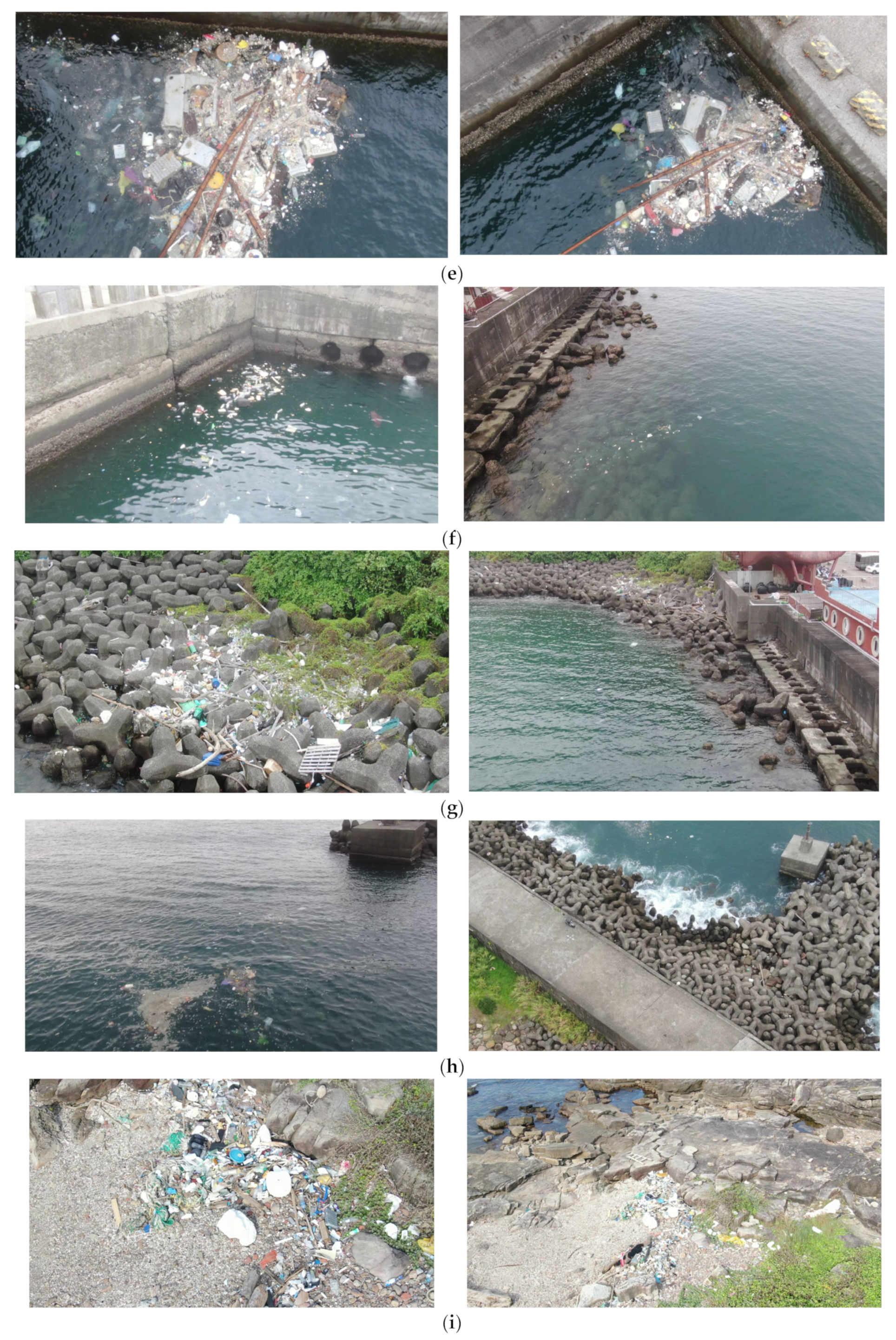
We created a trash dataset of 1319 aerial images called HAIDA, which includes two classes (3904 garbage objects and 2517 bottle objects) and 456 negative samples (without garbage and bottle objects) that were collected by UAVs [42]. The challenge to the coastal trash detection task is that such trash has no geometrical shape, and it is difficult for people to define and label the dataset, as shown in Figure 1. The ground sample distance (GSD) is 0.7 cm/pixel when the flight height of the UAV is 10 m.
In the HAIDA trash dataset, the images of trash in Taiwan were collected by UAVs. The bottle is the first class of the HAIDA dataset. In Figure 2a, such bottles were captured by a UAV from heights of 3 and 10 m on the campus of the National Taiwan Ocean University (NTOU). Garbage is the second class in the HAIDA trash dataset. We consider this garbage as plastic trash with no clear shape definition (unlike bottles). In Figure 2b, the bottles were captured by a UAV from heights of 3 and 5 m on the coastline of the NTOU. In Figure 2c–h, the garbage and the bottles were captured at 3 to 30 m heights in the Badouzi fishing port. In Figure 2i, the garbage and the bottles were captured by a UAV at 6 and 15 m heights along the Gongliao beach coastline. Figure 3 shows the negative samples in the HAIDA trash dataset.
- B.
- Object Detectors
Scaled-YOLOv4 is currently the state-of-the-art object detector based on CSPNet and YOLOv4. A comparison of average precision (AP) and latency for the state-of-the-art object detectors is shown in Figure 4.
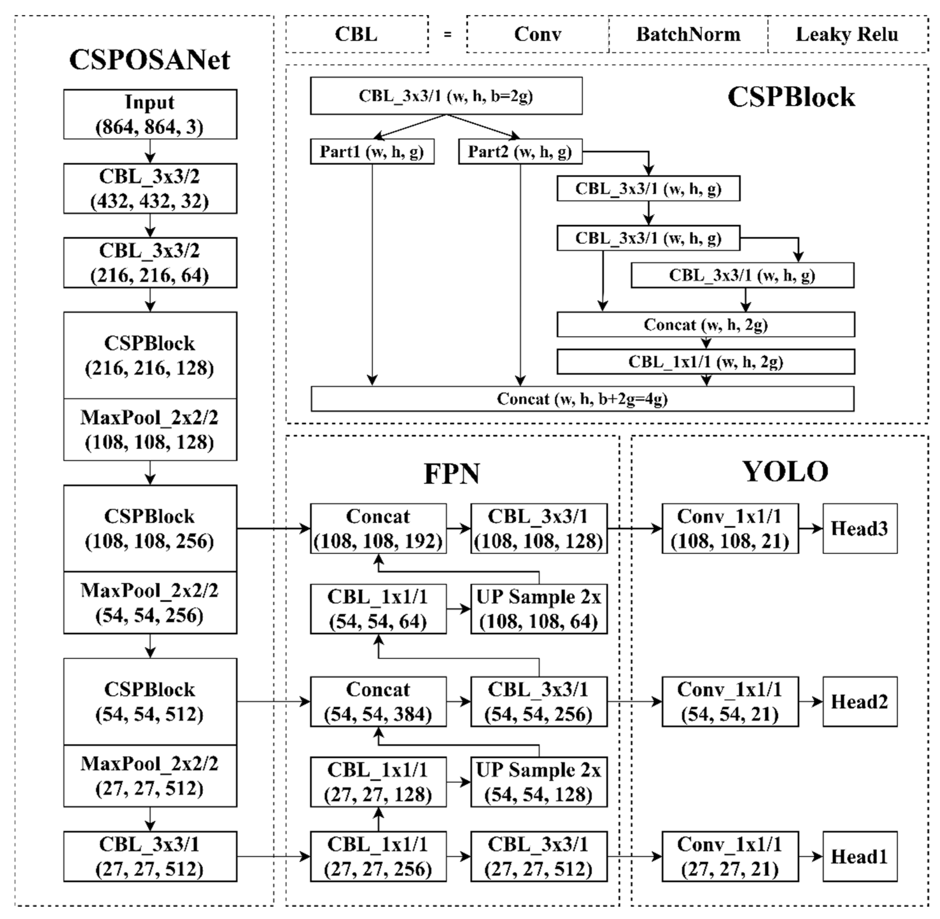
The backbone of YOLOv4-Tiny is CSPOSANet, which is inspired by CSPNet and VoVNet [31]. In VoVNet, the authors proposed a one-shot aggregation (OSA) module that concatenated all features only once in the last feature map to resolve the heavy memory cost (MAC) and the inefficiency of the computation of DenseNet [21], as shown in Figure 5.
There are three CSP blocks followed by max pool layers in CSPOSANet, as shown in Figure 6. The FPN structure is used in YOLOv4-Tiny-3l to integrate the feature maps and obtain more semantic information like with YOLOv3. YOLOv4-Tiny-3l uses three YOLO heads to predict objects across scales like YOLOv4 but does not use multiple anchors to predict per object; YOLOv4-Tiny-3l uses one anchor to fit one object. YOLOv4-Tiny [15] achieves the best performance in SOTA tiny models, as shown in Table 1.
- C.
- Holdout Method and Hyperparameter Tuning
The three-way holdout method is a simple way to select the best model for a trash detector. The dataset is split into three parts: a training set for model fitting, a validation set for both hyperparameter tuning and model selection, and a testing set for model evaluation, as shown in Figure 7.
In this study, the dataset was split for the holdout method as 70/20/10 into three parts. With hyperparameter tuning, when the input size was up to , the YOLOv4-Tiny-3l model achieved 71.46% AP50 (Val) on the validation set and obtained an inference speed of 22 frames per second (fps) on the NVIDIA embedded system Xavier NX. This result is better than that of YOLOv4 with 1.17% AP50 (Val) and (416) 12 fps. All models were trained on NVIDIA GeForce RTX-2080Ti GPU. Table 2 shows the performance of SOTA object detectors on the HAIDA trash dataset. Table 3 shows the hyperparameter tuning results for the YOLOv4-Tiny-3l model.
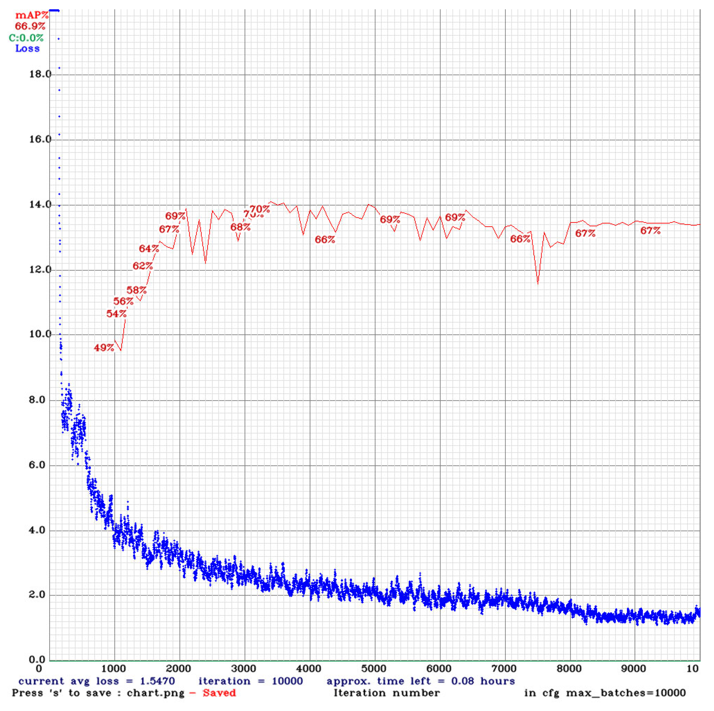
For the holdout method, considering the speed/accuracy tradeoff to UAV applications, we chose YOLOv4-Tiny-3l (864) as the best model over YOLOv4 (416), YOLOv4 (512), and YOLOv4 (608). YOLOv4-Tiny-3l (864) was better than YOLOv4 (416) at 6.76% AP50 on the HAIDA training set and could learn 97.41% of the dataset after training, as shown in Figure 8. The blue line is the loss of the training set, and the red line is the AP50 of the validation set. YOLOv4 (416) overfitted the training data after 3500 iterations, and the loss converged at 9000 iterations but obtained low AP50 (Val), as shown in Figure 9. To prevent overfitting of YOLOv4 (416), we used the model that obtained the best AP50 (Val) at 3500 iterations.
For the hyperparameter tuning of the YOLOv4-Tiny-3l model (864), we tried 13 factors to tune the model. These included the input size, batch size, iteration, learning rate, learning rate scheduler (multistep decay), multiscale training, Mosaic data augmentation, activation functions, self-adversarial training (SAT), IoU loss, NMS, and pretrained weight. The hardware of VRAM of RTX 2080Ti GPU limited the input and batch sizes. The learning rates of hyperparameter sets 6 and 12 were 0.00261 and 0.002, and the performances were 71.46% and 71.18%, respectively, as shown in Table 3. The multiscale training improved the 0.83% AP50 (Val). The steps and scales were parameters of the learning rate scheduler (multistep decay). The performances of hyperparameter set-1 and set-2 were 69.71% and 69.33%, respectively. The Leaky ReLU activation was better than the Mish by 0.88%. With Mosaic, SAT, and DIoU-NMS, these performances decreased by 0.31%, 0.73%, and 0.3%, respectively. The pretrained weights of ImageNet improved the AP50 (Val) by 2.25% and were better than the TACO [42] pretrained weights. In our experiments, the best hyperparameter set of YOLOv4-Tiny-3l (864) for the HAIDA trash dataset is shown in Table 3.
- D.
- K-Fold Cross-Validation
The result of the holdout method is sensitive to how we split the data. If there is a large bias in the dataset, the result of the holdout method will be affected, especially for small datasets. In Table 2, the AP50 (Val) and AP50 (Test) in YOLOv4 (416) are very different due to the bias in the HAIDA dataset. To obtain a better result for model evaluation, k-fold cross-validation [41] was used. First, the data were split into k parts, one part for the validation set, the remaining k1 parts for the training set, and repeated k times, as shown in Figure 10. Here, we chose k = 5 for our customized trash dataset. The YOLOv4 (416) model obtained the best average AP50 (test fold) 71.77% across five folds, and we could see the bias occur especially for YOLOv4-Tiny-3l (864), as shown in Table 4. The average AP50’s of YOLOv4-Tiny-3l (864) and YOLOv4 (416) were 71.45% and 71.77%, respectively. Considering the fast inference speed, the YOLOv4-Tiny-3l model was chosen as the trash detector.
- E.
- Nested Cross-Validation
Nested cross-validation [43] is a better method for simultaneous model evaluation and hyperparameter tuning. In our previous work, we used the holdout method to tune the hyperparameters of YOLOv4-Tiny-3l and YOLOv4 and discovered a bias in the HAIDA trash dataset. Thus, we used the hyperparameters’ tuned models to conduct model evaluations. However, a problem was that the hyperparameters are tuned based on the holdout method rather than the k-fold approach. Thus, we felt that nested cross-validation should be used to conduct more accurate model evaluations.
Nested cross-validation includes the outer and inner loop; the outer loop and inner loop are divided into k1 and k2 folds like the k-fold cross-validation. First, the inner loop is used to tune the hyperparameters, and the best one is chosen. Subsequently, these hyperparameters are applied to the outer loop for the model evaluation. This is repeated k1 times, and the errors are averaged, as shown in Figure 11 (k1 = 5 and k2 = 2).
Although the nested cross-validation is very accurate, it is time-consuming, especially for CNN. The cost of nested cross-validation is n k1 k2 m, where n is the number of models, k1 and k2 are the numbers of folds in the outer and inner loops, and m is the number of hyperparameter sets to compare in each inner loop. Nested cross-validation is used in linear regression, logistic regression, small neural networks, and support vector machines. In CNN, k-fold cross-validation is used for the small and medium datasets. The holdout method is commonly used for ImageNet and other large datasets.
3. Experimental Results
The YOLOv4-Tiny-3l model was implemented and utilized in the NVIDIA embedded system Xavier NX on the quadrotor. The total weight of the quadrotor was 5.05 kg with a flight duration of 21.8 min at an average speed of 2 (m/s) for patrolling the coastline. The onboard camera was at a 1080p resolution with a 30 fps video streaming ability, and the horizontal and vertical views were 65 and 70 degrees, respectively. Three areas (NTOU campus, Badouzi fishing port, and Wanghai Xiang beach) were tested, and the results are shown below.
- The NTOU Campus
First, we tested the regular shape trash (bottles) to see the outcomes in small object detection. The confidence scores of small object detections are high (98.27%, 64.65%, 91.86%), which means that the HAIDA dataset has a small bias to a real-world test on the NTOU campus, as shown in Figure 12 [44].
- B.
- Badouzi Fishing Port
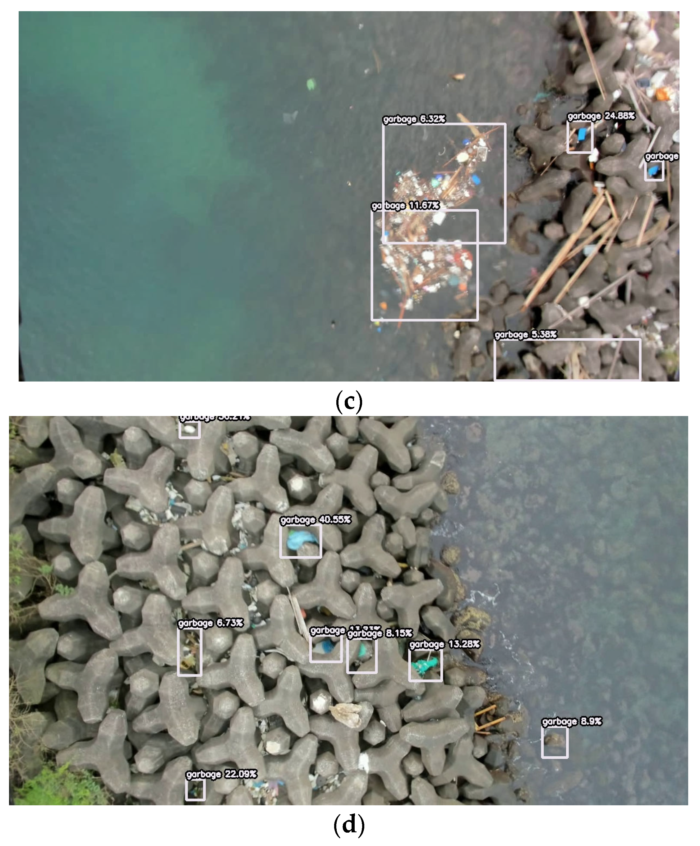
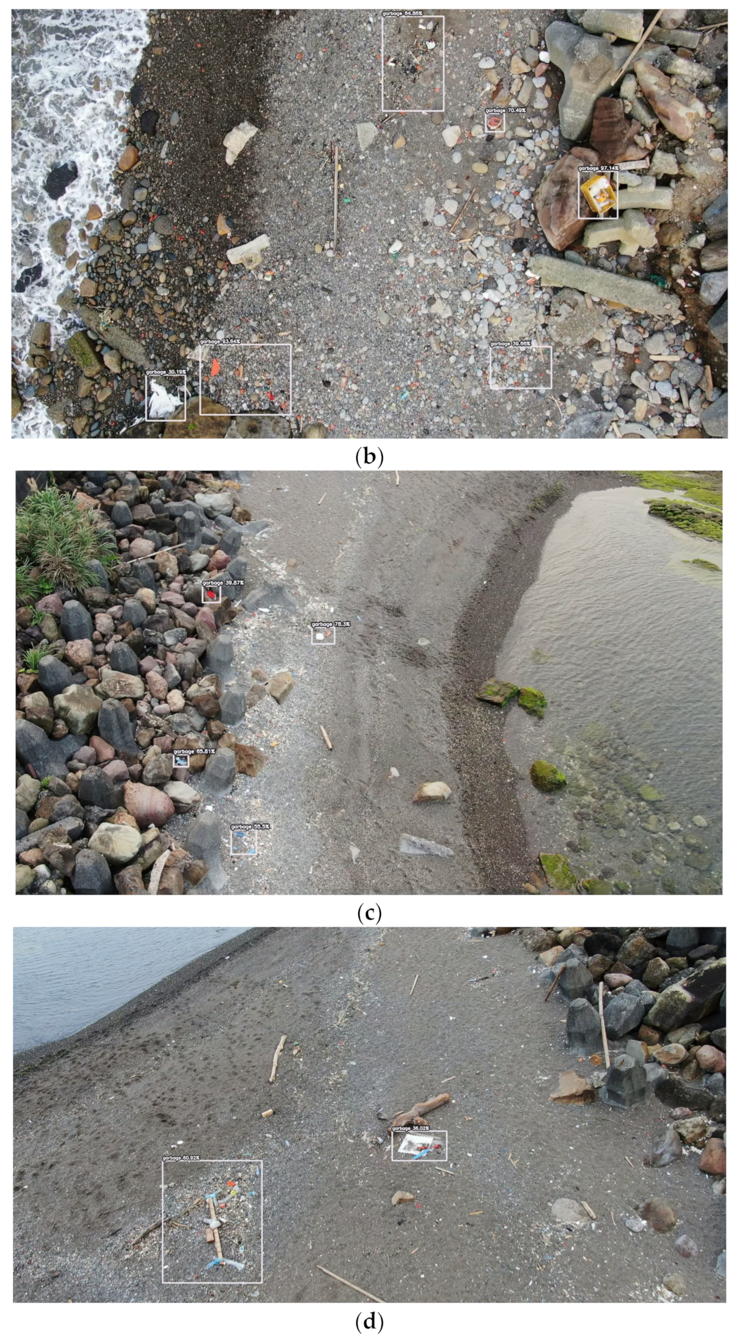
In the Badouzi fishing port, the shape and the texture of the garbage varied due to natural erosion. This decreased the confidence scores of garbage detection. This means that the HAIDA dataset had a large bias with respect to the Badouzi fishing port. The best solution to solve this problem was to collect more data. The YOLOv4-Tiny-3l model was trained from the HAIDA dataset, and the UAV flew at a height of 10 m, as shown in Figure 13a. Figure 13b–d shows the detection of large, medium, and small objects.
- C.
- Wanghai Xiang Beach
There was more plastic debris on the Wanghai Xiang beach, which easily confused both human detection and the trash detector to result in false-positive (FP) detection, as shown in Figure 14. The YOLOv4-Tiny-3l model was trained from the HAIDA dataset, and the UAV flew at a height of 5 m.
- D.
- Data Mining
The performance of the model is dependent on the data. We had a TACO trash dataset, which was collected by anonymous providers from different places. We also downloaded some trash data from the internet (crawler trash dataset). Further, we collected some aerial images from our UAV (simple aerial trash dataset). Due to the disorganized data content of beach trash, human error was highly probable in trash labeling. This led us to explore the impact of the dataset on the target detection task from the initial aerial shot dataset. For data mining, we used the holdout method to divide the dataset into a training set and a validation set (70% and 30%, respectively). YOLOv4 was trained for data mining and tested with the HAIDA trash dataset. After training, YOLOv4 obtained 99% mean average precision (mAP) on the simple aerial trash validation set, as shown in Figure 15. We used the TACO dataset (for segmentation) and relabeled it for object detection. After training, YOLOv4 obtained 83% mAP on the TACO validation, set as shown in Figure 16. We also used the dataset from the internet (crawler trash dataset) and labeled it for object detection. After training, YOLOv4 obtained 58% mAP on the crawler trash validation, set as shown in Figure 17.
We needed the model to predict the diverse trash types in multiple scales with good precision. The TACO and crawler datasets were not suitable for our UAV trash detector. We added some new aerial trash images collected by the UAV to the HAIDA dataset. We called it the HAIDA-2 trash dataset. There were 1880 aerial images with two classes (6179 garbage objects and 2563 bottle objects) and 556 negative samples. Figure 18 shows the HAIDA-2 trash dataset that was detected by YOLOv4-Tiny-3l (864).
After all trash was detected, the images of marked trash, the location of the trash, and the area of trash were then computed via the onboard computer of the UAV. This information was subsequently transmitted to the remote site computer through the Kafka connector and Mongo database [43]. A trash heatmap could be displayed on the monitor screen of the remote site computer for usage by an environmental protection agency, as shown in Figure 19 [43].
The real-time trash detection results were sent to the ground monitoring station, as shown in Figure 19a. The red flags are the target waypoints in the UAV monitoring mission. For the trash information, the blue markers indicate where the trash is detected, and the circle area presents the severity (color based on the trash polluted area table, as shown on the bottom left of Figure 19a) of the trash pollution area. The purple circles are the flight trajectory of the UAV, and the UAV status dashboard is shown on the right-hand side of Figure 19a. The trash information is saved in the database to query the data for the heatmap analysis for potential use by an environmental protection agency, as shown in Figure 19b. The heatmap also points out the severity of the trash pollution in the Badouzi fishing port. In the future, the overall heatmap analysis can potentially cover all coastal areas of Taiwan.
4. Conclusions
The holdout method and hyperparameter tuning were used to find the best object detector for our HAIDA trash dataset. The YOLOv4-tiny-3l trash detector was better than the YOLOv4 model for the HAIDA dataset when the input size was up to 864 864. We also employed the trash detector in an NVIDIA embedded system, NX, on the UAV to test the trash detector in three areas. The performances were good in the NTOU campus and the Badouzi fishing port scenarios. However, in the Wanghai Xiang beach scenario, there were some false-positive (FP) detections due to confusing debris. In this study, we implement the application of a UAV for marine trash detection with our previously published UAV trash monitoring system. This can contribute to global environmental protection. In the real-world test, the confidence scores of the trash detection at the Wanghai Xiang beach and the Badouzi fishing port were low (5% to 50%). This could be due to the trash detector using its generalization to predict the eroded trash, which has varying shapes. In future work, we will increase the confidence scores of the trash detector and filter out the low confidence scores with NMS and avoid FP detection by collecting more coastal trash data for detector training. In addition, aerial image quality is another key point in efficient trash detection. As the image was disturbed by the vibration from the UAV, this point also needs to be addressed in future studies.
Author Contributions
Conceptualization, Y.-H.L. and J.-G.J.; methodology, Y.-H.L. and J.-G.J.; software, Y.-H.L.; validation, Y.-H.L. and J.-G.J.; formal analysis, Y.-H.L. and J.-G.J.; investigation, Y.-H.L. and J.-G.J.; resources, Y.-H.L. and J.-G.J.; data curation, Y.-H.L.; writing—original draft preparation, Y.-H.L.; writing—review and editing, J.-G.J.; visualization, Y.-H.L. and J.-G.J.; supervision, J.-G.J.; project administration, J.-G.J.; funding acquisition, J.-G.J. All authors have read and agreed to the published version of the manuscript.
Funding
This research was funded by Ministry of Science and Technology (Taiwan), grant number MOST 110-2221-E-019-075-MY2. The APC was funded by the National Taiwan Ocean University and the Ministry of Science and Technology.
Institutional Review Board Statement
Not applicable.
Informed Consent Statement
Not applicable.
Data Availability Statement
Not applicable.
Conflicts of Interest
The authors declare no conflict of interest.
References
- Greenpeace. 2019. Available online: https://www.greenpeace.org/taiwan/update/15198 (accessed on 15 August 2020).
- 422 Earth Day. 2021. Available online: https://www.businesstoday.com.tw/article/category/183027/post/202104210017 (accessed on 5 May 2021).
- Schölkopf, B. SVMs-A Practical Consequence of Learning Theory. Proc. IEEE Intell. Syst. Appl. 1998, 13, 18–21. [Google Scholar]
- Gongde, G.; Hui, W.; David, B.; Yaxin, B.; Kieran, G. KNN Model-Based Approach in Classification. In Lecture Notes in Computer Science; Springer: Berlin/Heidelberg, Germany, 2003; Volume 2888, pp. 986–996. [Google Scholar] [CrossRef]
- Nielsen, H. Theory of the Backpropagation Neural Network. In Proceedings of the International 1989 Joint Conference on Neural Networks, Washington, DC, USA, 17–21 June 1989; Volume 1, pp. 593–605. [Google Scholar]
- Krizhevsky, A.; Sutskever, I.; Hinton, G.E. ImageNet Classification with Deep Convolutional Neural Networks. Commun. ACM 2017, 60, 84–90. [Google Scholar] [CrossRef] [Green Version]
- Liu, W.; Wei, J.; Meng, Q. Comparisons on KNN, SVM, BP and the CNN for Handwritten Digit Recognition. In Proceedings of the 2020 IEEE International Conference on Advances in Electrical Engineering and Computer Applications, Dalian, China, 25–27 August 2020; pp. 587–590. [Google Scholar]
- Ruchi; Singla, J.; Singh, A.; Kaur, H. Review on Artificial Intelligence Techniques for Medical Diagnosis. In Proceedings of the 3rd International Conference on Intelligent Sustainable Systems, Thoothukudi, India, 3–5 December 2020; pp. 735–738. [Google Scholar]
- Sermanet, P.; Eigen, D.; Zhang, X.; Mathieu, M.; Fergus, R.; LeCun, Y. OverFeat: Integrated Recognition, Localization and Detection using Convolutional Networks. In Proceedings of the 2nd International Conference on Learning Representations, Scottsdale, Arizona, 15–17 December 2013. [Google Scholar]
- Girshick, R.; Donahue, J.; Darrell, T.; Malik, J. Rich Feature Hierarchies for Accurate Object Detection and Semantic Segmentation. In Proceedings of the IEEE Computer Society Conference on Computer Vision and Pattern Recognition, Columbus, OH, USA, 23–28 June 2014; pp. 580–587. [Google Scholar]
- Redmon, J.; Divvala, S.; Girshick, R.; Farhadi, A. You Only Look Once: Unified, Real-Time Object Detection. In Proceedings of the IEEE Computer Society Conference on Computer Vision and Pattern Recognition, Las Vegas, NV, USA, 27–30 June 2016; pp. 779–788. [Google Scholar]
- Redmon, J.; Farhadi, A. YOLO9000: Better, Faster, Stronger. In Proceedings of the 30th IEEE Conference on Computer Vision and Pattern Recognition, Honolulu, HI, USA, 21–26 July 2017; pp. 6517–6525. [Google Scholar]
- Redmon, J.; Farhadi, A. YOLOv3: An Incremental Improvement. arXiv 2018, arXiv:1804.02767. Available online: http://arxiv.org/abs/1804.02767 (accessed on 5 August 2020).
- Bochkovskiy, A.; Wang, C.Y.; Liao, H.Y.M. YOLOv4: Optimal Speed and Accuracy of Object Detection. arXiv 2020, arXiv:2004.10934. [Google Scholar]
- Wang, C.; Liao, H.Y.M. Scaled-YOLOv4: Scaling Cross Stage Partial Network. arXiv 2020, arXiv:2011.08036. [Google Scholar]
- Ioffe, S.; Szegedy, C. Batch normalization: Accelerating Deep Network Training by Reducing Internal Covariate Shift. In Proceedings of the 32nd International Conference on Machine Learning, Mountain View, CA, USA, 6–11 July 2015; Volume 1, pp. 448–456. [Google Scholar]
- He, K.; Zhang, X.; Ren, S.; Sun, J. Deep Residual Learning for Image Recognition. In Proceedings of the IEEE Computer Society Conference on Computer Vision and Pattern Recognition, Las Vegas, NV, USA, 27–30 June 2016; pp. 770–778. [Google Scholar]
- Lin, T.Y.; Dollár, P.; Girshick, R.; He, K.; Hariharan, B.; Belongie, S. Feature Pyramid Networks for Object Detection. In Proceedings of the 30th IEEE Conference on Computer Vision and Pattern Recognition, CVPR 2017, Honolulu, HI, USA, 21–26 July 2017; pp. 936–944. [Google Scholar]
- Wang, C.Y.; Liao, H.Y.M.; Wu, Y.H.; Chen, P.Y.; Hsieh, J.W.; Yeh, I.H. CSPNet: A New Backbone that can Enhance Learning Capability of CNN. In Proceedings of the IEEE/CVF conference on computer vision and pattern recognition workshops, Seattle, WA, USA, 14–19 June 2020. [Google Scholar]
- Xie, S.; Girshick, R.; Dollár, P.; Tu, Z.; He, K. Aggregated Residual Transformations for Deep Neural Networks. In Proceedings of the 30th IEEE Conference on Computer Vision and Pattern Recognition, CVPR 2017, Honolulu, HI, USA, 21–26 July 2017; pp. 5987–5995. [Google Scholar]
- Huang, G.; Liu, Z.; van der Maaten, L.; Weinberger, K.Q. Densely Connected Convolutional Networks. In Proceedings of the 30th IEEE Conference on Computer Vision and Pattern Recognition, CVPR 2017, Honolulu, HI, USA, 21–26 July 2017; pp. 2261–2269. [Google Scholar]
- Liu, S.; Qi, L.; Qin, H.; Shi, J.; Jia, J. Path Aggregation Network for Instance Segmentation. In Proceedings of the IEEE Computer Society Conference on Computer Vision and Pattern Recognition, Salt Lake City, UT, USA, 18–23 June 2018; pp. 8759–8768. [Google Scholar]
- He, K.; Zhang, X.; Ren, S.; Sun, J. Spatial Pyramid Pooling in Deep Convolutional Networks for Visual Recognition. Lecture Notes in Computer Science (including subseries Lecture Notes in Artificial Intelligence and Lecture Notes in Bioinformatics). IEEE Trans. Pattern Anal. Mach. Intell. 2015, 37, 1904–1916. [Google Scholar] [CrossRef] [PubMed] [Green Version]
- Misra, D. Mish: A Self Regularized Non-Monotonic Activation Function. arXiv 2019, arXiv:1908.08681. Available online: http://arxiv.org/abs/1908.08681 (accessed on 25 July 2020).
- Ghiasi, G.; Lin, T.Y.; Le, Q.V. DropBlock: A Regularization Method for Convolutional Networks. Adv. Neural Inf. Process. Syst. 2018, 31, 10727–10737. [Google Scholar]
- Zhang, H.; Cisse, M.; Dauphin, Y.N.; Lopez-Paz, D. Mixup: Beyond Empirical Risk Minimization. In Proceedings of the 6th International Conference on Learning Representations, ICLR 2018-Conference Track Proceedings, Vancouver, BA, Canada, 30 April–3 May 2017. [Google Scholar]
- DeVries, T.; Taylor, G.W. Improved Regularization of Convolutional Neural Networks with Cutout. arXiv 2017, arXiv:1708.04552. Available online: http://arxiv.org/abs/1708.04552 (accessed on 12 July 2020).
- Yun, S.; Han, D.; Oh, S.J.; Chun, S.; Choe, J.; Yoo, Y. CutMix: Regularization Strategy to Train Strong Classifiers with Localizable Features. In Proceedings of the IEEE International Conference on Computer Vision, 27–28 October 2019; pp. 6022–6031. [Google Scholar]
- Rezatofighi, H.; Tsoi, N.; Gwak, J.; Sadeghian, A.; Reid, I.; Savarese, S. Generalized Intersection over Union: A Metric and A Loss for Bounding Box Regression. In Proceedings of the IEEE Computer Society Conference on Computer Vision and Pattern Recognition, Long Beach, CA, USA, 15–20 June 2019; pp. 658–666. [Google Scholar]
- Zheng, Z.; Wang, P.; Liu, W.; Li, J.; Ye, R.; Ren, D. Distance-IoU Loss: Faster and Better Learning for Bounding Box Regression. In Proceedings of the 34th AAAI Conference on Artificial Intelligence, Honolulu, HI, USA, 27 January–1 February 2019; pp. 12993–13000. [Google Scholar]
- Lee, Y.; Hwang, J.; Lee, S.; Bae, Y.; Park, J. An Energy and GPU-Computation Efficient Backbone Network for Real-Time Object Detection. In Proceedings of the IEEE Computer Society Conference on Computer Vision and Pattern Recognition Workshops, Long Beach, CA, USA, 16–17 June 2019; pp. 752–760. [Google Scholar]
- Bak, S.H.; Hwang, D.H.; Kim, H.M.; Yoon, H.J. Detection and Monitoring of Beach Litter using UAV Image and Deep Neural Network. Int. Arch. Photogramm. Remote Sens. Spat. Inf. Sci.-ISPRS Arch. 2019, 42, 55–58. [Google Scholar] [CrossRef] [Green Version]
- Badrinarayanan, V.; Kendall, A.; Cipolla, R. SegNet: A Deep Convolutional Encoder-Decoder Architecture for Image Segmentation. IEEE Trans. Pattern Anal. Mach. Intell. 2017, 39, 2481–2495. [Google Scholar] [CrossRef] [PubMed]
- Merlino, S.; Paterni, M.; Berton, A.; Massetti, L. Unmanned Aerial Vehicles for Debris Survey in Coastal Areas: Long-Term Monitoring Programme to Study Spatial and Temporal Accumulation of the Dynamics of Beached Marine Litter. Remote Sens. 2020, 12, 1260. [Google Scholar] [CrossRef] [Green Version]
- Escobar-Sánchez, G.; Haseler, M.; Oppelt, N.; Schernewski, G. Efficiency of Aerial Drones for Macrolitter Monitoring on Baltic Sea Beaches. Front. Environ. Sci. 2021, 8, 560237. [Google Scholar] [CrossRef]
- Tharani, M.; Amin, A.W.; Maaz, M.; Taj, M. Attention Neural Network for Trash Detection on Water Channels. arXiv 2020, arXiv:2007.04639. [Google Scholar]
- Proença, P.F.; Simões, P. TACO: Trash Annotations in Context for Litter Detection. arXiv 2020, arXiv:2003.06975. Available online: http://arxiv.org/abs/2003.06975 (accessed on 22 January 2021).
- Flickr. pedropro/TACO: Trash Annotations in Context Dataset Toolkit. Available online: https://github.com/pedropro/TACO (accessed on 21 March 2021).
- Liu, Y.; Ge, Z.; Lv, G.; Wang, S. Research on automatic garbage detection system based on deep learning and narrowband internet of things. J. Phys. 2018, 1069, 12032. [Google Scholar] [CrossRef] [Green Version]
- Niu, G.; Li, J.; Guo, S.; Pun, M.O.; Hou, L.; Yang, L. SuperDock: A deep learning-based automated floating trash monitoring system. In Proceedings of the 2019 IEEE International Conference on Robotics and Biomimetics (ROBIO), Dali, China, 6–8 December 2019; pp. 1035–1040. [Google Scholar]
- Raschka, S. Model Evaluation, Model Selection, and Algorithm Selection in Machine Learning. arXiv 2018, arXiv:1811.12808. Available online: http://arxiv.org/abs/1811.12808 (accessed on 5 August 2020).
- Ca, B.U.; Fr, Y.G. No Unbiased Estimator of the Variance of K-Fold Cross-Validation Yoshua Bengio Yves Grandvalet. J. Mach. Learn. Res. 2004, 16, 1–17. [Google Scholar]
- Wainer, J.; Cawley, G. Nested Cross-Validation When Selecting Classifiers Is Overzealous for Most Practical Applications. arXiv 2018, arXiv:1809.09446. Available online: http://arxiv.org/abs/1809.09446 (accessed on 23 July 2020). [CrossRef]
- Liao, Y.; Juang, J. Real-Time UAV Trash Monitoring System. Appl. Sci. 2022, 12, 1838. [Google Scholar] [CrossRef]
Figure 1.
HAIDA trash dataset.

Figure 2.
Garbage and bottles in the HAIDA trash dataset. (a) Bottles on the campus of the NTOU at heights of 3 and 10 m. (b) Bottles on the coastline of the NTOU at heights of 3 and 5 m. (c) Garbage and bottles in the Badouzi fishing port at heights of 4 and 10 m. (d) Garbage and bottles in the Badouzi fishing port at heights of 20 and 30 m. (e) Garbage in the Badouzi fishing port at heights of 3 and 7 m. (f) Garbage in the Badouzi fishing port at heights of 3 and 12 m. (g) Garbage and bottles in the Badouzi fishing port at heights of 7 and 15 m. (h) Garbage and bottles in the Badouzi fishing port at heights of 10 and 30 m. (i) Garbage in the Gongliao beach at heights of 6 and 15 m.


Figure 3.
Negative samples in the HAIDA trash dataset. (a) Negative samples in the Badouzi fishing port at heights of 7 and 30 m. (b) Negative samples in the Badouzi fishing port at heights of 15 and 10 m.
Figure 3.
Negative samples in the HAIDA trash dataset. (a) Negative samples in the Badouzi fishing port at heights of 7 and 30 m. (b) Negative samples in the Badouzi fishing port at heights of 15 and 10 m.

Figure 4.
Comparison of state-of-the-art object detectors on the MS COCO dataset, C.Y. Wang 2020.

Figure 5.
The structure of DenseNet and VoVNet, Z. Zheng 2019.

Figure 6.
The structure of YOLOv4-Tiny-3l.

Figure 7.
The three-way holdout method.

Figure 8.
The performance of YOLOv4-Tiny-3l (864) in the HAIDA dataset.

Figure 9.
The performance of YOLOv4 (416) in the HAIDA dataset.

Figure 10.
k-Fold cross-validation.

Figure 11.
Nested cross-validation.

Figure 12.
Real-world UAV tested on the NTOU campus.

Figure 13.
Trash detection at the Badouzi fishing port. (a) Real-world UAV test in Badouzi. (b) The detection result of the trash detector at location 1. (c) The detection result of the trash detector at location 2. (d) The detection result of the trash detector at location 3.
Figure 13.
Trash detection at the Badouzi fishing port. (a) Real-world UAV test in Badouzi. (b) The detection result of the trash detector at location 1. (c) The detection result of the trash detector at location 2. (d) The detection result of the trash detector at location 3.


Figure 14.
Trash detection at Wanghai Xiang beach. (a) The detection result of the trash detector at location 1. (b) The detection result of the trash detector at location 2. (c) The detection result of the trash detector at location 3.
Figure 14.
Trash detection at Wanghai Xiang beach. (a) The detection result of the trash detector at location 1. (b) The detection result of the trash detector at location 2. (c) The detection result of the trash detector at location 3.


Figure 15.
The performance of YOLOv4 on the simple aerial trash dataset.

Figure 16.
The performance of YOLOv4 on the TACO and simple aerial trash dataset.

Figure 17.
The performance of YOLOv4 on the crawler and simple aerial trash dataset.

Figure 18.
The detection results in the HAIDA-2 trash dataset by YOLOv4-Tiny-3l (864).


Figure 19.
Trash information and heatmap with the location. (a) Trash polluted area with detailed trash information in the Badouzi fishing port. (b) The heatmap of detected trash in the Badouzi fishing port.
Figure 19.
Trash information and heatmap with the location. (a) Trash polluted area with detailed trash information in the Badouzi fishing port. (b) The heatmap of detected trash in the Badouzi fishing port.


Table 1.
The performance of SOTA tiny models in the COCO dataset, C.Y. Wang 2020.
| Model | Size | FPS1080ti | FPSTX2 | AP |
|---|---|---|---|---|
| YOLOv4-tiny | 416 | 371 | 42 | 21.7% |
| YOLOv4-tiny(31) | 320 | 252 | 41 | 28.7% |
| ThunderS146 | 320 | 248 | - | 23.6% |
| CSPPeleeRef | 320 | 205 | 41 | 23.5% |
| YOLOv3-tiny | 416 | 368 | 37 | 16.6% |
Table 2.
Comparison of state-of-the-art object detectors on the HAIDA trash dataset.
| Method | Size | FPS 2080Ti | FPS NX | BFLOPs | AP30 (Val) | AP50 (Val) | AP75 (Val) | AP50 (Test) | AP50 (Train) |
|---|---|---|---|---|---|---|---|---|---|
| YOLOv4-Tiny-3l | 416 | 470 | 72 | 8.022 | 75.76% | 67.42% | 23.53% | 71.65% | 92.48% |
| YOLOv3-Tiny | 864 | 231 | 28 | 23.506 | - | 64.46% | - | 68.50% | 91.22% |
| YOLOv4-Tiny | 864 | 204 | 25 | 29.284 | - | 69.75% | - | 72.48% | 91.80% |
| YOLOv3-Tiny-3l | 864 | 194 | 24 | 30.639 | - | 66.15% | - | 69.85% | 91.97% |
| YOLOv4-Tiny-3l | 864 | 177 | 22 | 34.602 | 78.17% | 71.46% | 28.27% | 73.37% | 97.41% |
| YOLOv3 | 416 | 118 | 12 | 65.312 | - | 66.27% | - | 69.24% | 94.61% |
| YOLOv3-SPP | 416 | 116 | 12 | 65.69 | - | 64.66% | - | 66.86% | 90.88% |
| YOLOv4 | 416 | 92 | 10 | 59.57 | 78.36% | 70.29% | 29.15% | 74.20% | 90.65% |
| YOLOv4-CSP | 512 | 88 | 9 | 76.144 | - | 58.12% | - | 61.76% | 58.08% |
| YOLOv4 | 512 | 80 | 7 | 90.237 | 79.83% | 72% | 27.49% | 74.41% | 93.43% |
| YOLOv4 | 608 | 63 | 5 | 127.248 | 80.04% | 72.20% | 28.81% | 72.70% | 94.28% |
| YOLOv4x-MISH | 640 | 41 | 3 | 220.309 | 74.07% | 66.10% | 26.49% | 71.35% | 96.06% |
Table 3.
Hyperparameter sets for the YOLOv4-Tiny-3l model tuning.
| Hyperparameter. | Size | Batch | Iteration | lr | Steps | Scales | Multi-Scale | Act. | Mosaic | SAT | IOU | NMS | Pretrain | AP50 (Val) |
|---|---|---|---|---|---|---|---|---|---|---|---|---|---|---|
| 1 | 864 | 16 | 10,000 | 0.00261 | 4500; 7000 | 0.1; 0.1 | - | leaky | - | - | ciou | greedy | imageNet | 69.71% |
| 2 | 864 | 16 | 10,000 | 0.00261 | 8000; 9000 | 0.1; 0.1 | - | leaky | - | - | ciou | greedy | imageNet | 69.33% |
| 3 | 864 | 16 | 10,000 | 0.00261 | 8000; 9000 | 0.1; 0.1 | - | leaky | yes | - | ciou | greedy | imageNet | 70.69% |
| 4 | 864 | 16 | 10,000 | 0.00261 | 8000; 9000 | 0.1; 0.1 | - | leaky | yes | - | ciou | greedy | - | 68.07% |
| 5 | 864 | 8 | 10,000 | 0.00261 | 8000; 9000 | 0.1; 0.1 | yes | leaky | yes | - | ciou | greedy | imageNet | 71.15% |
| 6 | 864 | 8 | 10,000 | 0.00261 | 8000; 9000 | 0.1; 0.1 | yes | leaky | - | - | ciou | greedy | imageNet | 71.46% |
| 7 | 864 | 16 | 10,000 | 0.00261 | 8000; 9000 | 0.1; 0.1 | - | leaky | yes | - | ciou | greedy | imageNet | 70.32% |
| 8 | 864 | 8 | 10,000 | 0.00261 | 8000; 9000 | 0.1; 0.1 | - | leaky | yes | - | ciou | greedy | imageNet | 69.55% |
| 9 | 864 | 8 | 10,000 | 0.00261 | 8000; 9000 | 0.1; 0.1 | yes | leaky | - | - | ciou | diou | imageNet | 71.16% |
| 10 | 864 | 8 | 10,000 | 0.00261 | 8000; 9000 | 0.1; 0.1 | yes | leaky | - | yes | ciou | greedy | imageNet | 70.73% |
| 11 | 864 | 6 | 10,000 | 0.00261 | 8000; 9000 | 0.1; 0.1 | yes | mish | - | - | ciou | greedy | imageNet | 70.58% |
| 12 | 864 | 8 | 10,000 | 0.002 | 8000; 9000 | 0.1; 0.1 | yes | leaky | - | - | ciou | greedy | imageNet | 71.18% |
| 13 | 864 | 8 | 10,000 | 0.00261 | 8000; 9000 | 0.1; 0.1 | yes | leaky | - | - | ciou | greedy | TACO | 70.38% |
| 14 | 864 | 8 | 10,000 | 0.004 | 4500; 6000 | 0.1; 0.1 | - | leaky | - | - | ciou | greedy | imageNet | 71.25% |
Table 4.
Comparison of three models for five-fold cross-validation.
| Method | Size | AP50 (Test Fold) | |||||
|---|---|---|---|---|---|---|---|
| 5–1 | 5–2 | 5–3 | 5–4 | 5–5 | Avg. | ||
| YOLOv4-Tiny-3l | 864 | 73.61% | 71.28% | 68.89% | 73.72% | 69.76% | 71.45% |
| YOLOv4 | 416 | 72.56% | 72.48% | 70.80% | 72.45% | 70.58% | 71.77% |
| YOLOv4 | 512 | 72.63% | 71.31% | 70.18% | 73.58% | 70.67% | 71.67% |
Disclaimer/Publisher’s Note: The statements, opinions and data contained in all publications are solely those of the individual author(s) and contributor(s) and not of MDPI and/or the editor(s). MDPI and/or the editor(s) disclaim responsibility for any injury to people or property resulting from any ideas, methods, instructions or products referred to in the content. |
© 2023 by the authors. Licensee MDPI, Basel, Switzerland. This article is an open access article distributed under the terms and conditions of the Creative Commons Attribution (CC BY) license (https://creativecommons.org/licenses/by/4.0/).
Share and Cite
MDPI and ACS Style
Liao, Y.-H.; Juang, J.-G. Automatic Marine Debris Inspection. Aerospace 2023, 10, 84. https://doi.org/10.3390/aerospace10010084
AMA Style
Liao Y-H, Juang J-G. Automatic Marine Debris Inspection. Aerospace. 2023; 10(1):84. https://doi.org/10.3390/aerospace10010084
Chicago/Turabian StyleLiao, Yu-Hsien, and Jih-Gau Juang. 2023. "Automatic Marine Debris Inspection" Aerospace 10, no. 1: 84. https://doi.org/10.3390/aerospace10010084
Note that from the first issue of 2016, this journal uses article numbers instead of page numbers. See further details here.